On the Diversity-Multiplexing Tradeoff of Unconstrained Multiple-Access Channels

Abstract

In this work the optimal diversity-multiplexing tradeoff (DMT) is investigated for the multiple-input multiple-output fading multiple-access channel with no power constraints (infinite constellations). For $K$ users ($K>1$), $M$ transmit antennas for each user, and $N$ receive antennas, infinite constellations in general and lattices in particular are shown to attain the optimal DMT of finite constellations for $N\geq(K+1)M-1$, i.e., user limited regime. On the other hand for $N<\left(K+1\right)M-1$ it is shown that infinite constellations can not attain the optimal DMT. This is in contrast to the point-to-point case in which infinite constellations are DMT optimal for any $M$ and $N$. In general, this work shows that when the network is heavily loaded, i.e., $K>\max\left(1,\frac{N-M+1}{M}\right)$, taking into account the shaping region in the decoding process plays a crucial role in pursuing the optimal DMT. By investigating the cases in which infinite constellations are optimal and suboptimal, this work also gives a geometrical interpretation to the DMT of infinite constellations in multiple-access channels.

I Introduction

Employing multiple antennas in a point-to-point wireless channel increases the number of degrees of freedom available for transmission. This is illustrated for the ergodic case in [1],[2], where $M$ transmit and $N$ receive antennas increase the capacity by a factor of $\min\left(M,N\right)$. The number of degrees of freedom utilized by the transmission scheme is referred to as multiplexing gain. Another advantage of employing multiple antennas is the potential increase in the transmitted signal reliability. The fact that multiple antennas increase the number of independent links between antenna pairs, enables the error probability to decrease, i.e., add diversity. If for high signal to noise ratio ($\mathsf{SNR}$) the error probability is proportional to $\mathsf{SNR}^{-d}$, then we state that the diversity order is $d$.

For the point-to-point setting, Zheng and Tse [3] characterized the optimal diversity-multiplexing tradeoff (DMT) of the quasi-static Rayleigh flat-fading channel, i.e., for each multiplexing gain they found the best attainable diversity order. The optimal DMT is a piecewise linear function connecting the points $\left(M-l\right)\left(N-l\right)$, $l=0,\dots,\min\left(M,N\right)$. The transmission scheme in [3] uses random codes. Subsequent works presented more structured schemes that attain the optimal DMT. El Gamal et al. [4] showed by using probabilistic methods that lattice space-time (LAST) codes attain the optimal DMT by using minimum-mean square error (MMSE) estimation followed by lattice decoding. Later, explicit coding schemes based on lattices and cyclic-division algebra [5], [6] were shown to attain the optimal DMT by using maximum-likelihood (ML) decoding, and also by using MMSE estimation followed by lattice decoding [7]. A subtle but very important point is that these coding schemes take into consideration the finiteness of the codebook in the decoder. A question that remained open was whether lattices can achieve the optimal DMT by using regular lattice decoding, i.e., decoder that takes into account the infinite lattice without considering the shaping region or the power constraint. In order to answer this question, the work in [8] presented an analysis of the performance of infinite constellations (IC’s) in multiple-input multiple-output (MIMO) fading channels. A new tradeoff was presented between the IC’s average number of dimensions per channel use, i.e., the IC dimensionality divided by the number of channel uses, and the best attainable DMT. By choosing the right average number of dimensions per channel use, it was shown [8] that IC’s in general and more specifically lattices using regular lattice decoding, attain the optimal DMT of finite constellations.

For the multiple-access channel, where a number of users transmit to a single receiver, the number of users in the network affects the multiplexing gain and the diversity order. For instance, for a network with $K$ users transmitting at the same rate, the number of available degrees of freedom for each user is $\min\left(M,\frac{N}{K}\right)$. Tse, Viswanath and Zheng [9] characterized the optimal DMT of a network with $K$ users, where each user has $M$ transmit antennas and the receiver has $N$ antennas. For the symmetric case, in which the users transmit at the same multiplexing gain $r$, i.e., $r_{1}=\dots=r_{K}=r$, the optimal DMT takes the following elegant form [9]:

• For $r\in\left[0,\min\left(\frac{N}{K+1},M\right)\right]$ the optimal symmetric DMT equals to the optimal DMT of a point-to-point channel with $M$ transmit and $N$ receive antennas $d^{\ast,\left(FC\right)}_{M,N}\left(r\right)$.

• For $r\in\left[\min\left(\frac{N}{K+1},M\right),\min\left(M,\frac{N}{K}\right)\right]$ the optimal symmetric DMT equals to the optimal DMT of a point-to-point channel with all $K$ users pulled together $d^{\ast,\left(FC\right)}_{K\cdot M,N}\left(Kr\right)$.

Similar to the development in the point-to-point case, random codes were used in [9]. Later Nam and El Gamal [10] showed that a random ensemble of LAST codes attains the optimal DMT of the multiple-access channel using MMSE estimation followed by lattice decoding over the lattice induced by the $K$ users. An explicit coding scheme based on lattices and cyclic division algebra that attains the optimal DMT using ML decoding was presented in [11].

In this paper we study the optimal DMT of lattices using regular lattice decoding, i.e., decoding without taking into consideration the power constraint, for the MIMO Rayleigh fading multiple-access channel. The result is rather surprising; unlike the point-to-point case in which the tradeoff between dimensions and diversity enables to attain the optimal DMT, we show that for the multiple-access channel the optimal DMT is attained only for $N\geq\left(K+1\right)M-1$, i.e., user limited regime. On the other hand when the network is heavily loaded we show that IC’s or lattices using regular lattice decoding, can not attain the optimal DMT.

In the first part of this paper an upper bound on the optimal symmetric DMT IC’s can achieve is derived. The upper bound is attained by finding for each multiplexing gain $r$, the average number of dimensions per channel use for each user, that maximizes the diversity order. In the case $N<\left(K+1\right)M-1$ it is shown that the optimal DMT of IC’s does not coincide with the optimal DMT of finite constellations. Moreover, for $N<\left(K-1\right)M+1$ it is shown that the optimal DMT of IC’s in the symmetric case is inferior compared to the optimal DMT of finite constellations, for any value of $r$ except for the edges $r=0$, $\frac{N}{K}$. On the other hand for $N\geq(K+1)M-1$, by choosing the correct average number of dimensions per channel use for each user, it is shown that the upper bound on the optimal DMT of IC’s coincides with the optimal DMT of finite constellations $d^{\ast,\left(FC\right)}_{M,N}\left(\max\left(r_{1},\dots,r_{K}\right)\right)$.

In the second part of this paper, a transmission scheme that attains the optimal DMT for $N\geq(K+1)M-1$ is presented. Each user in this scheme transmits according to the DMT optimal scheme for the point-to-point channel, presented in [8]. By analyzing the receiver joint ML decoding performance, it is shown that this transmission scheme attains the optimal DMT of finite constellations. We wish to emphasize that the proposed transmission scheme is more involved than simply using orthogonalization between users, which in general is shown to be suboptimal for IC’s. The proposed transmission scheme requires $N+M-1$ channel uses to attain the optimal DMT, which is smaller than $N+KM-1$, the number of channel uses required in [9] (the dependence in the number of users lies in the fact that $N\geq\left(K+1\right)M-1$). Finally, the algebraic analysis of the transmission scheme geometrically explains why for $N\geq(K+1)M-1$ the optimal DMT equals to the optimal DMT of the point-to-point channel of each user, i.e., why the optimal DMT equals $d^{\ast,\left(FC\right)}_{M,N}\left(\max\left(r_{1},\dots,r_{K}\right)\right)$.

As a basic illustrative example for the results we consider the following two cases. For the first case assume a network with two users ($K=2$), where each user has a single transmit antenna ($M=1$), and a receiver with a single receive antenna ($N=1$). In this case the optimal DMT of finite constellations in the symmetric case [9] equals $1-r$ for $r\in\left[0,\frac{1}{3}\right]$, and $2-4r$ for $r\in\left[\frac{1}{3},\frac{1}{2}\right]$. For IC’s it is shown in this setting that the optimal DMT for the symmetric case equals $1-2r$ for $r\in\left[0,\frac{1}{2}\right]$, which is strictly inferior except for $r=0$, $\frac{1}{2}$. In the second case, by merely adding another receive antenna, i.e., $M=1$, $N=K=2$, the optimal DMT of IC’s coincides with finite constellations optimal DMT $d^{\ast,\left(FC\right)}_{1,2}\left(\max\left(r_{1},r_{2}\right)\right)$.

It is important to note that for $N<\left(K+1\right)M-1$ this paper shows the sub-optimality of IC’s compared to the optimal DMT of finite constellations. However, in this case an explicit analytical expression for the upper bound on the optimal DMT of IC’s is given only for the symmetric case, whereas for the general case the upper bound is presented in the form of optimization problem. Indeed, for $N<\left(K+1\right)M-1$ it still remains an open problem to find an explicit expression for the general upper bound (the non-symmetric case) on the optimal DMT of IC’s, together with a transmission scheme that achieves it. On the other hand, when $N\geq\left(K+1\right)M-1$ this paper provides both analytical upper bound to the optimal DMT of IC’s, and also a transmission scheme that attains it.

The outline of the paper is as follows. In section II basic definitions for the fading multiple-access channel and IC’s are given. Section III presents an upper bound on the optimal DMT of IC’s, and shows the sub-optimality of IC’s for $N<\left(K+1\right)M-1$. Transmission scheme that attains the optimal DMT of finite constellations for $N\geq\left(K+1\right)M-1$ is presented in section IV. Finally, in section V we discuss the results in this paper and present for the multiple-access channel a geometrical interpretation to the DMT of IC’s.

II Basic Definitions

II-A Channel Model

We consider a $K$-user multiple access channel for which each user has $M$ transmit antennas, and the receiver has $N$ antennas. We assume perfect knowledge of all channels at the receiver, and no channel knowledge at the transmitters. We also assume quasi static flat-fading channel for each user. The channel model is as follows:

$$\underline{y}_{t}=\sum_{i=1}^{K}H^{\left(i\right)}\cdot\underline{x}_{t}^{\left(i\right)}+\rho^{-\frac{1}{2}}\underline{n}_{t}\qquad t=1,\dots,T$$ (1)

where $\underline{x}_{t}^{\left(i\right)}$, $t=1,\dots,T$ is user $i$ transmitted signal, $\underline{n}_{t}\sim\mathcal{CN}(\underline{0},\frac{2}{2\pi e}I_{N})$ is the additive noise for which $\mathcal{CN}$ denotes complex-normal, $I_{N}$ is the $N$-dimensional unit matrix, and $\underline{y}_{t}\in\mathbb{C}^{N}$. $H^{\left(i\right)}$ is the fading matrix of user $i$. It consists of $N$ rows and $M$ columns, where $h^{\left(i\right)}_{l,j}\sim\mathcal{CN}(0,1)$, $1\leq l\leq N$, $1\leq j\leq M$, are the entries of $H^{\left(i\right)}$. The scalar $\rho^{-\frac{1}{2}}$ multiplies each element of $\underline{n}_{t}$, where $\rho$ can be interpreted as the average $\mathsf{SNR}$ of each user at the receive antennas for power constrained constellations that satisfy $\frac{1}{T}\sum_{t=1}^{T}E\{\lVert\underline{x}^{\left(i\right)}_{t}\rVert^{2}\}\leq\frac{2}{2\pi e}$.

Next we wish to define an equivalent channel to (1). Let us define the extended transmission vector

$$\underline{x}=\left(\underline{x}_{1}^{\left(1\right)\dagger},\dots,\underline{x}_{1}^{\left(K\right)\dagger},\dots,\underline{x}_{T}^{\left(1\right)\dagger},\dots,\underline{x}_{T}^{\left(K\right)\dagger}\right)^{\dagger}$$ (2)

i.e., first concatenate the users in each channel use, and then concatenate the vectors between channel uses. Now we define $H=\left(H^{\left(1\right)},\dots,H^{\left(K\right)}\right)$ which is an $N\times KM$ matrix. By defining $H_{ex}$ as an $NT\times KMT$ block diagonal matrix for which each block on the diagonal equals $H$, $\underline{n}_{\mathrm{ex}}=\rho^{-\frac{1}{2}}\cdot\left(\underline{n}_{1}^{\dagger},\dots,\underline{n}_{T}^{\dagger}\right)^{\dagger}\in\mathbb{C}^{NT}$ and $\underline{y}_{\mathrm{ex}}\in\mathbb{C}^{NT}$, we can rewrite the channel model in (1)

$$\underline{y}_{\mathrm{ex}}=H_{\mathrm{ex}}\cdot\underline{x}+\underline{n}_{\mathrm{ex}}.$$ (3)

Let $L=\min\left(N,KM\right)$, and let $\sqrt{\lambda}_{i}$, $1\leq i\leq L$ be the real valued, non-negative singular values of $H$. We assume $\sqrt{\lambda}_{L}\geq\dots\geq\sqrt{\lambda}_{1}>0$. For large values of $\rho$, we state that $f(\rho)\dot{\geq}g(\rho)$ when $\lim_{\rho\to\infty}\frac{\ln\left(f(\rho)\right)}{\ln(\rho)}\geq\frac{\ln\left(g(\rho)\right)}{\ln(\rho)}$, and also define $\dot{\leq}$, $\dot{=}$ in a similar manner by substituting $\geq$ with $\leq$, $=$ respectively.

II-B Infinite Constellations

Infinite constellation (IC) is a countable set $S=\{s_{1},s_{2},\dots\}$ in $\mathbb{C}^{n}$. Let $\mathrm{cube}_{l}(a)\subset\mathbb{C}^{n}$ be a (probably rotated) $l$-complex dimensional cube ($l\leq n$) with edge of length $a$ centered around zero. We define an IC $S_{l}$ to be $l$-complex dimensional if there exists rotated $l$-complex dimensional cube $\mathrm{cube}_{l}(a)$ such that $S_{l}\subset\lim_{a\to\infty}\mathrm{cube}_{l}(a)$ and $l$ is minimal. $M(S_{l},a)=|S_{l}\bigcap\mathrm{cube}_{l}(a)|$ is the number of points of the IC $S_{l}$ inside $\mathrm{cube}_{l}(a)$. In [12], the $n$-complex dimensional IC density was defined as

$$\gamma_{\mathrm{G}}=\limsup_{a\to\infty}\frac{M(S_{n},a)}{a^{2n}}$$

and the volume to noise ratio (VNR) for the additive white Gaussian noise (AWGN) channel was given as

$$\mu_{\mathrm{G}}=\frac{\gamma_{\mathrm{G}}^{-\frac{1}{n}}}{2\pi e\sigma^{2}}$$

where $\sigma^{2}$ is the noise variance of each component.

We now turn to the IC definitions at the transmitters. We define the average number of dimensions per channel use as the IC dimension divided by the number of channel uses. Let us consider user $i$, where $1\leq i\leq K$. We denote the average number of dimensions per channel use by $D_{i}$. Let us consider a $D_{i}T$-complex dimensional sequence of IC’s - $S^{\left(i\right)}_{D_{i}T}(\rho)$, where $D_{i}\leq M$, $T$ is the number of channel uses, and $\sum_{i=1}^{K}D_{i}\leq L$. First we define $\gamma_{tr}^{\left(i\right)}=\rho^{r_{i}T}$ as the density of $S_{KT}^{\left(i\right)}(\rho)$ at transmitter $i$. Similarly to the definitions in [8] the multiplexing gain of user’s $i$ IC is defined as

$$r_{i}=\lim_{\rho\to\infty}\frac{1}{T}\log_{\rho}(\gamma_{\mathrm{tr}}^{\left(i\right)}+1)=\lim_{\rho\to\infty}\frac{1}{T}\log_{\rho}(\rho^{r_{i}T}+1),\quad 0\leq r_{i}\leq D_{i}.$$ (4)

The VNR at the transmitter of user $i$ is

$$\mu_{\mathrm{tr}}^{{}^{\left(i\right)}}=\frac{{\gamma_{\mathrm{tr}}^{\left(i\right)}}^{-\frac{1}{D_{i}T}}}{2\pi e\sigma^{2}}=\rho^{1-\frac{r_{i}}{D_{i}}}$$ (5)

where $\sigma^{2}=\frac{\rho^{-1}}{2\pi e}$ is each component’s additive noise variance. Now let us concatenate the users IC’s in accordance with (2). We denote $D=\sum_{i=1}^{K}D_{i}$. The concatenation yields an equivalent $DT$-complex dimensional IC, $S_{D\cdot T}\left(\rho\right)$, that has multiplexing gain $\sum_{i=1}^{K}r_{i}$, density $\gamma_{tr}=\rho^{\left(\sum_{i=1}^{K}r_{i}\right)T}$ and VNR $\mu_{tr}=\rho^{1-\frac{\sum_{i=1}^{K}r_{i}}{D}}$. In this case we get in (3) that the transmitted signal $\underline{x}\in S_{DT}\left(\rho\right)\subset\mathbb{C}^{KMT}$.

At the receiver we first define the set $H_{ex}\cdot cube_{D\cdot T}(a)$ as the multiplication of each point in $cube_{D\cdot T}(a)$ with the matrix $H_{ex}$. In a similar manner, the IC induced by the channel at the receiver is $S_{D\cdot T}^{{}^{\prime}}=H_{ex}\cdot S_{D\cdot T}$. The set $H_{ex}\cdot cube_{D\cdot T}(a)$ is almost surely $D\cdot T$-complex dimensional (where $D\leq L$). In this case

$${M(S_{D\cdot T},a)=|S_{D\cdot T}\bigcap\mathrm{cube}_{D\cdot T}(a)|=|S_{D\cdot T}^{{}^{\prime}}\bigcap(H_{ex}\cdot\mathrm{cube}_{D\cdot T}(a))|.}$$

We define the receiver density as

$$\gamma_{\mathrm{rc}}=\limsup_{a\to\infty}\frac{M(S_{D\cdot T},a)}{\mathbf{Vol}(H_{ex\cdot}\mathrm{cube}_{D\cdot T}(a))}$$

i.e., the upper limit on the ratio of the number of IC points in $H_{ex}\cdot\mathrm{cube}_{D\cdot T}(a)$, and the volume of $H_{ex}\cdot\mathrm{cube}_{D\cdot T}(a)$. Note that for $N\geq KM$ and $D=KM$ we get $\gamma_{\mathrm{rc}}=\rho^{\sum_{i=1}^{K}r_{i}T}\cdot\prod_{i=1}^{KM}\lambda_{i}^{-T}$ and $\mu_{\mathrm{rc}}=\rho^{1-\frac{\sum_{i=1}^{K}r_{i}}{KM}}\cdot\prod_{i=1}^{KM}\lambda_{i}^{\frac{1}{KM}}$. The joint decoder average decoding error probability, over the points of the effective IC $S_{D\cdot T}(\rho)$, for a certain channel realization $H$, is defined as

$$\overline{Pe}(H,\rho)=\limsup_{a\to\infty}\frac{\sum_{\underline{x}^{{}^{\prime}}\in S_{D\cdot T}^{{}^{\prime}}\bigcap(H_{ex}\cdot\mathrm{cube}_{D\cdot T}(a))}Pe(\underline{x}^{{}^{\prime}},H,\rho)}{M(S_{D\cdot T},a)}$$ (6)

where $Pe(\underline{x}^{{}^{\prime}},H,\rho)$ is the error probability associated with $\underline{x}^{{}^{\prime}}$. The average decoding error probability of $S_{D\cdot T}(\rho)$ over all channel realizations is $\overline{Pe}(\rho)=E_{H}\{\overline{Pe}(H,\rho)\}$. The diversity order is defined as

$$d=-\lim_{\rho\to\infty}\log_{\rho}(\overline{Pe}(\rho)).$$ (7)

In practice finite constellations are transmitted even when performing regular lattice decoding at the receiver. Based on the results in [13] it was shown in [8] that finite constellation with multiplexing gain $r$ can be carved from a lattice with multiplexing gain $r$, while maintaining the same performance when regular lattice decoder is employed at the receiver. In our case it also applies to each of the users, i.e., carving finite constellations with multiplexing gains tuple $\left(r_{1},\dots,r_{K}\right)$ that satisfy the power constraint, from lattices with multiplexing gains tuple $\left(r_{1},\dots,r_{K}\right)$. At the receiver the performance is maintained by performing regular lattice decoding on the effective lattice.

II-C Additional Notations

We further denote by $d^{\ast,\left(FC\right)}_{M,N}\left(r\right)$ the optimal DMT of finite constellations, and by $d^{\ast,D}_{M,N}\left(r\right)$ the upper bound on the optimal DMT of any IC with average number of dimensions per channel use $D$, both in a point to point channel with $M$ transmit and $N$ receive antennas. For the multiple access channel with $K$ users, $M$ transmit antennas for each user, and $N$ receive antennas, we denote by $d^{\ast,\left(FC\right)}_{K,M,N}\left(r\right)$ the optimal DMT of finite constellations in the symmetric case, and by $d^{\ast,\left(IC\right)}_{K,M,N}\left(r\right)$, $d^{\ast,\left(IC\right)}_{K,M,N}\left(r_{1},\dots,r_{K}\right)$ the upper bounds on the optimal DMT of the unconstrained multiple-access channel for the symmetric case, and for multiplexing gains tuple $\left(r_{1},\dots,r_{K}\right)$ respectively.

We denote $r_{max}=\max\left(r_{1},\dots,r_{K}\right)$, i.e., the maximal multiplexing gain in the multiplexing gains tuple. In addition for any $A\subseteq\left\{1,\dots,K\right\}$ we define $R_{A}=\sum_{a\in A}r_{a}$ and $D_{A}=\sum_{a\in A}D_{a}$.

III Upper Bound on the Best Diversity-Multiplexing Tradeoff

In this section we show that for $N<(K+1)M-1$ the DMT of the unconstrained multiple-access channel is suboptimal compared to the optimal DMT of finite constellations. On the other hand for $N\geq(K+1)M-1$, we derive an upper bound on the optimal DMT that coincides with the optimal DMT of finite constellations.

In subsection III-A we lower bound the error probability of any IC for the multiple-access channel, by using lower bounds on the error probability of any IC in the point-to-point channel. We use these lower bounds to formulate an upper bound on the optimal DMT of IC’s for the multiple-access channel, in the form of an optimization problem. In subsection III-B we solve this optimization problem for the symmetric case. We compare the optimal DMT of IC’s to the optimal DMT of finite constellations, and find the cases for which IC’s are suboptimal in subsection III-C. Finally in subsection III-D we give a convexity argument that shows for the symmetric case that whenever the optimal DMT is not a convex function IC’s are suboptimal

III-A Upper Bound on the Diversity-Multiplexing-Tradeoff

We lower bound the error probability of the unconstrained multiple-access channel in Lemma 1. Based on this lower bound we present in Theorem 2 an upper bound on the optimal DMT of IC’s.

Assume user $i$ transmits over $D_{i}T$-complex dimensional IC, with average number of dimensions per channel use $D_{i}$ and $T$ channel uses. The following lemma lower bounds the average decoding error probability of the $K$-users $\overline{Pe}^{\left(D_{1},\dots,D_{K},T\right)}\left(\rho,r_{1},\dots,r_{K}\right)$, where $\left(D_{1},\dots,D_{K}\right)$ is the tuple of average number of dimensions per channel use, $T$ is the number of channel uses and $\left(r_{1},\dots,r_{K}\right)$ is the tuple of multiplexing gains.

Lemma 1.

$${\overline{Pe}^{\left(D_{1},\dots,D_{K},T\right)}\left(\rho,r_{1},\dots,r_{K}\right)\geq\max_{A\subseteq\left\{1,\dots,K\right\}}\left(Pe^{\left(D_{A},T\right)}\left(\rho,R_{A}\right)\right)}$$

where $Pe^{\left(D_{A},T\right)}\left(\rho,R_{A}\right)$ is the lower bound derived in [8] for the error probability of any IC with $T$ channel uses, $D_{A}=\sum_{a\in A}D_{a}$ average number of dimensions per channel use, and multiplexing gain $R_{A}=\sum_{a\in A}r_{a}$, in a point-to-point channel with $|A|\cdot M$ transmit and $N$ receive antennas.

Proof.

By considering the extended channel model (3), we get that the $K$ distributed transmitters transmit an effective $\left(\sum_{i=1}^{K}D_{i}\right)T$-complex dimensional IC, over $T$ channel uses, with multiplexing gain $\sum_{i=1}^{K}r_{i}$. The error probability of this IC is lower bounded by the lower bound for the error probability of any IC with average number of dimensions per channel use $\sum_{i=1}^{K}D_{i}$, $T$ channel uses, and multiplexing gain $\sum_{i=1}^{K}r_{i}$, in a point-to-point channel with $KM$ transmit and $N$ receive antennas. Such a lower bound on the error probability was derived in [8] for each channel realization ([8] Theorem 1), and then for the average over all channel realizations when $\rho$ is large ([8] Theorem 2). Now consider the set $A\subset\left\{1,\dots,K\right\}$. In case a genie tells the receiver the transmitted messages of users $\left\{1,\dots,K\right\}\setminus A$, the optimal receiver attains an error probability that lower bounds the $K$-user optimal receiver error probability. Without loss of optimality, the optimal receiver can subtract them from the received signal, and get a new $|A|$-users unconstrained multiple-access channel with average number of dimensions per channel use $\left\{D_{a}\right\}_{a\in A}$, $T$ channel uses, and multiplexing gain $\sum_{a\in A}r_{a}$. In a similar manner, the error probability of this $|A|$-users channel is lower bounded by the lower bound on the error probability of any IC with $\sum_{a\in A}D_{a}$ average number of dimensions per channel use, $T$ channel uses, and multiplexing gain $\sum_{a\in A}r_{a}$, derived in [8]. Hence, the maximal lower bound on the error probability for $A\subseteq\left\{1,\dots,K\right\}$, also sets a lower bound for the error probability. This concludes the proof. ∎

Next we wish to formulate an upper bound on the DMT of IC’s in the $K$-user unconstrained multiple-access channel. We derive this bound based on the lower bound on the error probability presented in Lemma 1, and on an upper bound on the DMT of IC’s for the point-to-point channel, presented in [8]. Let us begin by presenting the upper bound on the DMT for the point-to-point channel.

Theorem 1 ([8] Theorem 2).

For any sequence of IC’s $S_{D\cdot T}\left(\rho\right)$ with $D$ average number of dimensions per channel use, in a point-to-point channel with $M$ transmit and $N$ receive antennas, the DMT $d^{D\cdot T}_{M,N}\left(r\right)$ is upper bounded by

$$d^{D\cdot T}_{M,N}\left(r\right)\leq d^{\ast,D}_{M,N}\left(r\right)=\frac{M\cdot N}{D}\left(D-r\right)$$

for $0\leq D\leq\frac{M\cdot N}{N+M-1}$, and

$$d^{D\cdot T}_{M,N}\left(r\right)\leq d^{\ast,D}_{M,N}\left(r\right)=\frac{\left(M-l\right)\left(N-l\right)}{D-l}\cdot\left(D-r\right)$$

for $\frac{M\cdot N-\left(l-1\right)l}{N+M-1-2\left(l-1\right)}\leq D\leq\frac{M\cdot N-l\left(l+1\right)}{N+M-1-2l}$, and $l=1,\dots,\min\left(M,N\right)-1$. In all cases $0\leq r\leq D$.

Based on Lemma 1 and Theorem 1 we formulate the following upper bound on the optimal DMT of the multiple-access channel.

Theorem 2.

The optimal DMT of any sequence of IC’s with multiplexing gains tuple $\left(r_{1},\dots,r_{K}\right)$ is upper bounded by

$$d^{\ast,\left(IC\right)}_{K,M,N}\left(r_{1},\dots,r_{K}\right)=\max_{\left(D_{1},\dots,D_{K}\right)\in\mathbf{D}}\min_{A\subseteq\left\{1,\dots,K\right\}}\left(d^{\ast,D_{A}}_{|A|\cdot M,N}\left(R_{A}\right)\right)$$

where $\mathbf{D}=\left\{D_{1},\dots,D_{K}\mid 0\leq D_{i}\leq M,\sum_{i=1}^{K}D_{i}\leq L\right\}$.

Proof.

Following Lemma 1 we get a lower bound for the error probability of any sequence of effective IC’s $S_{\sum_{i=1}^{K}D_{i}T}\left(\rho\right)$, transmitted by the $K$ users. This lower bound can be translated to an upper bound on the diversity order. In addition, this lower bound on the error probability depends on lower bounds on the error probabilities for the point-to-point channel. Hence, we can use the upper bound on the DMT in the point-to-point channel, presented in Theorem 1, to get the following upper bound on the DMT of a tuple of average number of dimensions per channel use $\left(D_{1},\dots,D_{K}\right)$

$$\min_{A\subseteq\left\{1,\dots,K\right\}}\left(d^{\ast,D_{A}}_{|A|\cdot M,N}\left(R_{A}\right)\right).$$

Maximizing over $\left(D_{1},\dots,D_{K}\right)\in\mathbf{D}$ yields the upper bound on the optimal DMT. ∎

III-B Characterizing the Optimal Symmetric DMT

We wish to characterize an upper bound on the optimal DMT of IC’s in the symmetric case, i.e., $r_{1}=\dots=r_{K}=r$. Later we will use this upper bound in order to show the sub-optimality of the unconstrained multiple-access channel in the case $N<\left(K+1\right)M-1$. In addition, we will show that the upper bound coincides with the optimal DMT of finite constellations in the case $N\geq\left(K+1\right)M-1$.

Lemmas 2, 3, 4, 5 present the relations between $d^{\ast,i\cdot D}_{i\cdot M,N}\left(i\cdot r\right)$, $i=1,\dots,K$ for different values of $N$. We use these lemmas in order to upper bound the optimal DMT in the symmetric case in Theorem 4.

Based on Theorem 2 we can state that the optimal DMT for the symmetric case for $K$ users is upper bounded by

$$d^{\ast,\left(IC\right)}_{K,M,N}\left(r\right)=\max_{\left(D_{1},\dots,D_{K}\right)\in\mathbf{D}}\min_{A\subseteq\left\{1,\dots,K\right\}}\left(d^{\ast,D_{A}}_{|A|\cdot M,N}\left(|A|\cdot r\right)\right)$$ (8)

where $0\leq r\leq\frac{L}{K}$, i.e., we wish solve the aforementioned optimization problem for each $0\leq r\leq\frac{L}{K}$. In order to solve this optimization problem we first solve a simpler optimization problem for the case $D_{1}=\dots=D_{K}=D$, i.e., each user transmits over $D$ average number of dimensions per channel use. In this case the upper bound in (8) takes a simpler form

$$\max_{D}\min_{1\leq i\leq K}\left(d^{\ast,i\cdot D}_{i\cdot M,N}\left(i\cdot r\right)\right)$$ (9)

where $0\leq D\leq\frac{L}{K}$. After solving this optimization problem, we will show that choosing $D_{1}=\dots=D_{K}=D$ also yields the optimal solution for (8).

In order to solve the optimization problem in (9), we first need to present some properties on the relations between $d^{\ast,i\cdot D}_{i\cdot M,N}\left(i\cdot r\right)$, $1\leq i\leq K$. We begin by presenting a property on the behavior of $d^{\ast,D}_{M,N}\left(\cdot\right)$ as a function of $D$.

Corollary 1 ([8] Corollary 1).

For $0\leq D\leq\frac{M\cdot N}{N+M-1}$ we have the following equality

$$d^{\ast,D}_{M,N}\left(0\right)=MN,$$

whereas for $\frac{M\cdot N-\left(l-1\right)l}{N+M+1-2\left(l-1\right)}\leq D\leq\frac{M\cdot N-l\left(l+1\right)}{N+M-1-2l}$, and $l=1,\dots,\min\left(M,N\right)-1$ we get

$$d^{\ast,D}_{M,N}\left(l\right)=(M-l)\cdot(N-l).$$

A simple interpretation of Corollary 1 is that for $0\leq D\leq\frac{M\cdot N}{N+M-1}$ the straight lines $d^{\ast,D}_{M,N}\left(\cdot\right)$ that represent the upper bounds on the DMT, all have the same “anchor” point at multiplexing gain $r=0$, i.e., they all have diversity order $MN$ at $r=0$, and each line equals to zero at $r=D$. On the other hand, for $\frac{M\cdot N-\left(l-1\right)\left(l\right)}{N+M+1-2l}\leq D\leq\frac{M\cdot N-\left(l\right)\left(l+1\right)}{N+M-1-2l}$, and $l=1,\dots,\min\left(M,N\right)-1$, the straight lines equal to $\left(M-l\right)\left(N-l\right)$ for multiplexing gain $r=l$, and again each line equals to zero for $r=D$. Figure 1 illustrates this property for $M=N=2$.

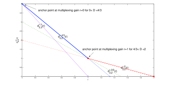
Figure 1: Upper bound on the DMT for any IC of $D$ average number of dimensions per channel use, in a point to point channel with $M=N=2$. Note that $d^{\ast,1}_{2,2}\left(r\right)$ and $d^{\ast,\frac{4}{3}}_{2,2}\left(r\right)$ are straight lines that equal to $MN=4$ at multiplexing gain $r=0$, whereas $d^{\ast,\frac{3}{2}}_{2,2}\left(r\right)$ and $d^{\ast,2}_{2,2}\left(r\right)$ are straight lines that equal to $\left(M-1\right)\left(N-1\right)=1$ at multiplexing gain $r=1$, in accordance with Corollary 1. In bold is the optimal DMT of finite constellations.

The next corollary presents the relation between $d^{\ast,D}_{M,N}\left(l\right)$ and $d^{\ast,\left(FC\right)}_{M,N}\left(r\right)$.

Corollary 2.

For any $0\leq D\leq\min\left(M,N\right)$ we have the following inequality

$$d^{\ast,D}_{M,N}\left(r\right)\leq d^{\ast,\left(FC\right)}_{M,N}\left(r\right)$$

for $0\leq r\leq D$. Furthermore, when $l\leq r\leq l+1$ and $l=0,\dots,\min\left(M,N\right)-1$

$$d^{\ast,\left(FC\right)}_{M,N}\left(r\right)=NM-l\cdot\left(l+1\right)-\left(N+M-1-2\cdot l\right)r.$$

Proof.

The proof follows from [8, Corollary 2] stating that for any $l=0,\dots,\min\left(M,N\right)-1$ and $l\leq r\leq l+1$

$$\max_{D}d^{\ast,D}_{M,N}\left(r\right)\leq d^{\ast,D_{l}}_{M,N}\left(r\right)=d^{\ast,\left(FC\right)}_{M,N}\left(r\right)$$

where $D^{\ast}_{l}=\frac{N\cdot M-l\cdot\left(l+1\right)}{N+M-1-2l}$. Therefore, for any $0\leq D\leq\left(M,N\right)-1$ we get

$$d^{\ast,D}_{M,N}\left(r\right)\leq d^{\ast,\left(FC\right)}_{M,N}\left(r\right).$$

for $0\leq r\leq D$.

The explicit expression for $d^{\ast,\left(FC\right)}_{M,N}\left(r\right)$ is obtained by the straight lines that connect the points $\left(l,\left(N-l\right)\cdot\left(M-l\right)\right)$ and $\left(l+1,\left(N-l-1\right)\cdot\left(M-l-1\right)\right)$, for $l=0,\dots,\min\left(M,N\right)-1$. ∎

Another property relates to the optimal DMT of finite constellations for the multiple-access channel in the symmetric case.

Theorem 3 ([9] Theorem 3).

The optimal DMT of finite constellations in the symmetric case equals

$$d^{\ast,\left(FC\right)}_{K,M,N}\left(r\right)=\left\{\begin{array}[]{lr}d^{\ast,\left(FC\right)}_{M,N}\left(r\right)&0\leq r\leq\min\left(\frac{N}{K+1},M\right)\\ d^{\ast,\left(FC\right)}_{KM,N}\left(K\cdot r\right)&\min\left(\frac{N}{K+1},M\right)\leq r\leq\min\left(\frac{N}{K},M\right)\end{array}\right.$$

In order to solve the optimization problem in (9) we present several lemmas related to the inequalities between $d^{\ast,i\cdot D}_{i\cdot M,N}\left(i\cdot r\right)$ for $1\leq i\leq K$. The proofs of these lemmas rely mainly on Corollary 1, Corollary 2 and Theorem 3.

Lemma 2.

For $N\geq\left(K+1\right)M-1$ we get

$$d^{\ast,D}_{M,N}\left(r\right)\leq d^{\ast,i\cdot D}_{i\cdot M,N}\left(i\cdot r\right)\quad 2\leq i\leq K$$

for any $0\leq r\leq D$ and $0\leq D\leq M$.

Proof.

The proof is in appendix A. ∎

An example for Lemma 2 for $M=K=2$ and $N=4$ is illustrated in Figure 2.

Figure 2: Illustration of Lemma 2 for the case $M=K=2$ and $N=5$. We compare the straight lines $d^{\ast,D}_{M,N}\left(r\right)$ and $d^{\ast,2D}_{2M,N}\left(2r\right)$ for $D=1$ and $D=\frac{3}{2}$. It can be seen that for this setting $d^{\ast,2D}_{2M,N}\left(2r\right)>d^{\ast,D}_{M,N}\left(r\right)$.

Lemma 3.

For $N<\left(K+1\right)M-1$ we get

$$d^{\ast,D}_{M,N}\left(r\right)\leq d^{\ast,i\cdot D}_{i\cdot M,N}\left(i\cdot r\right)\quad 2\leq i\leq K-1$$

for any $0\leq D\leq\frac{L}{K}$ and $0\leq r\leq D$.

Proof.

The proof is in appendix B ∎

From Lemmas 2, 3 we can see that the optimization problem in (9) involves only $d^{\ast,D}_{M,N}\left(r\right)$ and $d^{\ast,K\cdot D}_{K\cdot M,N}\left(K\cdot r\right)$. We now prove two more properties that will enable us to find the optimal DMT of IC’s in the symmetric case.

Lemma 4.

For $N<\left(K-1\right)M+1$ we get

$$\max_{0\leq D\leq\frac{L}{K}}\min_{1\leq i\leq K}d^{\ast,i\cdot D}_{i\cdot M,N}\left(i\cdot r\right)=d^{\ast,\frac{N}{K}}_{M,N}\left(r\right)=M\cdot N-M\cdot K\cdot r$$

where $0\leq r\leq\frac{N}{K}$.

Proof.

The proof is in appendix C ∎

From Lemma 4 we can see that for the multiple-access channel, when $N<\left(M-1\right)K+1$ the optimal DMT of IC’s is smaller than finite constellations optimal DMT for any value of $r$ except for $r=0$ and $r=\frac{N}{k}$. Figure 3 illustrates Lemma 4 for the case $M=N=K=2$. Now let us show the cases for which $d^{\ast,D}_{M,N}\left(r\right)$ and $d^{\ast,K\cdot D}_{K\cdot M,N}\left(K\cdot r\right)$ coincide.

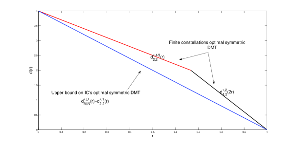
Figure 3: Illustration of Lemma 4 for the case $M=N=K=2$. In this case the optimal DMT is smaller than the optimal DMT of finite constellations, for any value of $r$ except for $r=0$, 1.

The following lemma serves as another building block in upper bounding the optimal DMT in the symmetric case when $N=\left(K-1\right)M+1+l$, $l=0,\dots,2M-3$. It finds the average number of dimensions per channel use that leads to the equality $d^{\ast,D}_{M,N}\left(r\right)=d^{\ast,K\cdot D}_{K\cdot M,N}\left(K\cdot r\right)$ for any value of $r$, and also shows for which values of $r$ these straight lines are equal to the optimal DMT of finite constellations in a point-to-point channel.

Lemma 5.

For $N=\left(K-1\right)M+1+l<\left(K+1\right)M-1$, where $l=0,\dots,2M-3$, we get for average number of dimensions per channel use per user $D_{l}=\frac{MN-\lfloor\frac{l}{2}\rfloor\cdot\left(\lfloor\frac{l}{2}\rfloor+1\right)-2\cdot\left(\lfloor\frac{l}{2}\rfloor+1\right)\cdot\left(\frac{l}{2}-\lfloor\frac{l}{2}\rfloor\right)}{N+M-1-l}$ that

$$d^{\ast,D_{l}}_{M,N}\left(r\right)=d^{\ast,K\cdot D_{l}}_{K\cdot M,N}\left(K\cdot r\right)=d^{\ast}\left(r\right)=MN-\lfloor\frac{l}{2}\rfloor\cdot\left(\lfloor\frac{l}{2}\rfloor+1\right)-2\cdot\left(\lfloor\frac{l}{2}\rfloor+1\right)\cdot\left(\frac{l}{2}-\lfloor\frac{l}{2}\rfloor\right)-\left(N+M-1-l\right)r$$

where $0\leq r\leq D_{l}$. In addition

$$d^{\ast,\left(FC\right)}_{M,N}\left(\lfloor\frac{l}{2}\rfloor+1\right)=d^{\ast}\left(\lfloor\frac{l}{2}\rfloor+1\right)$$

and also

$$d^{\ast,\left(FC\right)}_{KM,N}\left(\left(K-1\right)M+\lfloor\frac{l+1}{2}\rfloor\right)=d^{\ast}\left(\frac{\left(K-1\right)M+\lfloor\frac{l+1}{2}\rfloor}{K}\right)$$

Proof.

The proof is in appendix D. ∎

An example that illustrates Lemma 5 for $M=K=2$ and $N=4$ is given in Figure 4.

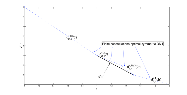
Figure 4: $d^{\ast}\left(r\right)$ for $M=K=2$ and $N=4$, i.e., $l=1$. Note that $d^{\ast}\left(1\right)=d^{\ast,8/5}_{2,4}\left(1\right)=d^{\ast,\left(FC\right)}_{2,4}\left(1\right)=d^{\ast,2}_{2,4}\left(1\right)$ and $d^{\ast}\left(\frac{3}{2}\right)=d^{\ast,4}_{4,4}\left(3\right)=d^{\ast,\left(FC\right)}_{4,4}\left(3\right)=d^{\ast,\frac{10}{3}}_{4,4}\left(3\right)$.

We are now are ready to characterize the upper bound on the optimal DMT of IC’s in the symmetric case. Recall that for $N=\left(K-1\right)M+1+l<\left(K+1\right)M-1$, $l=0,\dots,2M-3$

$$d^{\ast}\left(r\right)=MN-\lfloor\frac{l}{2}\rfloor\cdot\left(\lfloor\frac{l}{2}\rfloor+1\right)-2\cdot\left(\lfloor\frac{l}{2}\rfloor+1\right)\cdot\left(\frac{l}{2}-\lfloor\frac{l}{2}\rfloor\right)-\left(N+M-1-l\right)r.$$

Theorem 4.

The optimal DMT of any sequence of IC’s in the symmetric case is upper bounded by:
For $N\geq\left(K+1\right)M-1$

$$d^{\ast,\left(IC\right)}_{K,M,N}\left(r\right)=d^{\ast,\left(FC\right)}_{M,N}\left(r\right).$$

For $N<\left(K-1\right)M+1$

$$d^{\ast,\left(IC\right)}_{K,M,N}\left(r\right)=M\cdot N-K\cdot M\cdot r.$$

For $N=\left(K-1\right)M+1+l<\left(K+1\right)M-1$, where $l=0,\dots,2M-3$

$$d^{\ast,\left(IC\right)}_{K,M,N}\left(r\right)=\left\{\begin{array}[]{ll}d^{\ast,\left(FC\right)}_{M,N}\left(r\right)&0\leq r\leq\lfloor\frac{l}{2}\rfloor+1\\ d^{\ast}\left(r\right)&\lfloor\frac{l}{2}\rfloor+1\leq r\leq\frac{\left(K-1\right)M+\lfloor\frac{l+1}{2}\rfloor}{K}\\ d^{\ast,\left(FC\right)}_{KM,N}\left(Kr\right)&\frac{\left(K-1\right)M+\lfloor\frac{l+1}{2}\rfloor}{K}\leq r\leq\frac{L}{K}\end{array}\right.$$

Proof.

The proof is in appendix E. ∎

Figure 4 also presents $d^{\ast,\left(IC\right)}_{K,M,N}\left(r\right)$ for $M=K=2$ and $N=4$ (which leads to $l=1$).

III-C Comparison to Finite Constellations

In this subsection we compare the optimal DMT of finite constellations to the upper bound on the optimal DMT of IC’s (in general, not only for the symmetric case). This comparison enables us to show that for $N\geq\left(K+1\right)M-1$ the upper bound on the optimal DMT of IC’s coincides with the optimal DMT of finite constellations. On the other hand for $N<\left(K+1\right)M-1$ we show that the upper bound on the optimal DMT of IC’s is inferior compared to the optimal DMT of finite constellations. This leads to the conclusion that in the case $N<\left(K+1\right)M-1$, the best DMT any sequence of IC’s can attain is suboptimal compared to the optimal DMT of finite constellations.

In Lemma 6 we compare the upper bound on the optimal DMT of IC’s in the symmetric case, to the optimal DMT of finite constellations. Then we use this result to prove in Theorem 5 that the optimal DMT of IC’s is suboptimal when $N<\left(K+1\right)M-1$.

We begin by showing when the upper bound on the optimal DMT of IC’s in the symmetric case, $d^{\ast,\left(IC\right)}_{K,M,N}\left(r\right)$, is suboptimal compared to the optimal DMT of finite constellations.

Lemma 6.

For either $N\geq\left(K+1\right)M-1$ or $K=2$, $M=s+1$, $N=3\cdot s$, where $s\geq 1$ and $s\in\mathbb{Z}$ we get

$$d^{\ast,\left(IC\right)}_{K,M,N}\left(r\right)=d^{\ast,\left(FC\right)}_{K,M,N}\left(r\right).$$

For $N<\left(K-1\right)M+1$

$$d^{\ast,\left(IC\right)}_{K,M,N}\left(r\right)<d^{\ast,\left(FC\right)}_{K,M,N}\left(r\right)\quad 0<r<\frac{N}{K}.$$

For $N=\left(K-1\right)M+1+l<\left(K+1\right)M-1$ and $l=0,\dots,2M-3$

$$d^{\ast,\left(IC\right)}_{K,M,N}\left(r\right)<d^{\ast,\left(FC\right)}_{K,M,N}\left(r\right)$$

where $\lfloor\frac{l}{2}\rfloor+1<r<\frac{\left(K-1\right)M+\lfloor\frac{l+1}{2}\rfloor}{K}$.

Proof.

The full proof is in appendix F. In a nutshell the proof is based on the properties of $d^{\ast,D}_{M,N}\left(r\right)$ derived in Corollary 1 as well as Corollary 2, and also on the results in Theorem 4. It is important to note that for $K=2$, $M=s+1$ and $N=3\cdot s$ we get that $d^{\ast,\left(IC\right)}_{K,M,N}\left(r\right)=d^{\ast,\left(FC\right)}_{K,M,N}\left(r\right)$ because in this case $\lfloor\frac{l}{2}\rfloor+1=\frac{\left(K-1\right)M+\lfloor\frac{l+1}{2}\rfloor}{K}$. ∎

The sub-optimality of $d^{\ast,\left(IC\right)}_{K,M,N}\left(r\right)$ for $N<\left(K-1\right)M+1$ is illustrated in Figure 3, whereas the sub-optimality for $N=\left(K-1\right)M+1+l$ and $l=0,\dots,2m-3$ is illustrated in Figure 4.

We now present the cases for which the upper bound on the optimal DMT of the unconstrained multiple-access channel coincides with the optimal DMT of finite constellations, and the cases where the optimal DMT of the unconstrained multiple-access channel is suboptimal compared to the optimal DMT of finite constellations.

Theorem 5.

For $N\geq\left(K+1\right)M-1$ the optimal DMT of the unconstrained multiple-access channel is upper bounded by $d^{\ast,\left(FC\right)}_{M,N}\left(\max\left(r_{1},\dots,r_{K}\right)\right)$ the optimal DMT of finite constellations. In the case $N<\left(K+1\right)M-1$, the best DMT that can be attained for the unconstrained multiple-access channel is inferior compared to the optimal DMT of finite constellations.

Proof.

The full proof is in appendix G. The proof outline is as follows. Recall that in Theorem 2 we have shown that the optimal DMT of IC’s is upper bounded by

$$d^{\ast,\left(IC\right)}_{K,M,N}\left(r_{1},\dots,r_{K}\right)=\max_{\left(D_{1},\dots,D_{K}\right)\in\mathbf{D}}\min_{A\subseteq\left\{1,\dots,K\right\}}\left(d^{\ast,D_{A}}_{|A|\cdot M,N}\left(R_{A}\right)\right).$$

For $N\geq\left(K+1\right)M-1$ we show that this term is upper and lower bounded by $d^{\ast,\left(FC\right)}_{M,N}\left(\max\left(r_{1},\dots,r_{K}\right)\right)$, which is the optimal DMT of finite constellations in this case.

In the case $N<\left(K+1\right)M-1$ we show that the optimal DMT is not attained by finding a set of multiplexing gain tuples $\left(r_{1},\dots,r_{K}\right)\in B$ for which $d^{\ast,\left(IC\right)}_{K,M,N}\left(r_{1},\dots,r_{K}\right)<d^{\ast,\left(FC\right)}_{K,M,N}\left(r_{1},\dots,r_{K}\right)$. Based on Lemma 6 we get for $r_{1}=\dots=r_{K}=r$ that there exists a set of multiplexing gains for which $d^{\ast,\left(IC\right)}_{K,M,N}\left(r\right)<d^{\ast,\left(FC\right)}_{K,M,N}\left(r\right)$, except for $K=2$, $M=s+1$ and $N=3\cdot s$, where $s\geq 1$ is an integer. For this case showing that $d^{\ast,\left(IC\right)}_{2,s+1,3\cdot s}\left(r_{1},r_{2}\right)<d^{\ast,\left(FC\right)}_{2,s+1,3\cdot s}\left(r_{1},r_{2}\right)$ is more involved and requires considering the case $r_{1}\neq r_{2}$ (see appendix G for the full proof). An illustrative example for the method of proof for this case is presented in Figures 5, 6. ∎

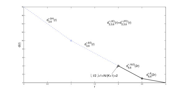
Figure 5: The upper bound on the optimal DMT of IC’s in the symmetric case for $K=2$, $M=3$, $N=6$. Note that for this case we get $\lfloor\frac{l}{2}\rfloor+1=\frac{N}{K+1}=\frac{\left(K-1\right)M+1+\lfloor\frac{l+1}{2}\rfloor}{K}$. In addition this upper bound coincides with the optimal DMT of finite constellations in the symmetric case. Finally, for this case we get $d^{\ast,\frac{8}{3}}_{3,6}\left(r\right)=d^{\ast,\frac{16}{3}}_{6,6}\left(2r\right)$ .

Figure 6: Illustration of the sub-optimality of the unconstrained multiple-access channel for $M=3$, $N=6$ and $K=2$. In this example we take $r_{1}=r_{0}+\epsilon=\frac{13}{6}+\frac{1}{24}$ and $r_{2}=r_{0}-\epsilon=\frac{13}{6}-\frac{1}{24}$, where $r_{0}=\frac{13}{6}$. In this case the optimal diversity order of finite constellations equals $\min\left(d^{\ast,\left(FC\right)}_{3,6}\left(r_{1}\right),d^{\ast,\left(FC\right)}_{3,6}\left(r_{2}\right),d^{\ast,\left(FC\right)}_{6,6}\left(r_{1}+r_{2}\right)\right)$. From the figure it can be seen that the minimum is obtained for $d^{\ast,\left(FC\right)}_{6,6}\left(r_{1}+r_{2}\right)=d^{\ast,\left(FC\right)}_{6,6}\left(2r_{0}\right)=3$. On the other hand IC’s diversity order equals $\min\left(d^{\ast,D_{1}}_{3,6}\left(r_{1}\right),d^{\ast,D_{2}}_{3,6}\left(r_{2}\right),d^{\ast,D_{1}+D_{2}}_{6,6}\left(2r_{0}\right)\right)$. In this example we choose $D_{1}=\frac{8}{3}+\frac{1}{6}$, $D_{2}=\frac{8}{3}-\frac{1}{6}$. In this case we get $d^{\ast,D_{1}+D_{2}}_{6,6}\left(2r_{0}\right)=d^{\ast,\frac{16}{3}}_{6,6}\left(2r_{0}\right)=3$, $d^{\ast,D_{1}}_{3,6}\left(r_{1}\right)=d^{\ast,\frac{17}{6}}_{3,6}\left(r_{1}\right)=3$ and $d^{\ast,D_{2}}_{3,6}\left(r_{2}\right)=d^{\ast,\frac{15}{6}}_{3,6}\left(r_{2}\right)=\frac{5}{2}<3$. Hence, in this case the diversity order of IC’s is smaller than the optimal diversity order of finite constellations. It results from the fact that for $0<D\leq\frac{8}{3}$ the straight lines $d^{\ast,D}_{3,6}\left(r\right)$ rotate around anchor points with multiplexing gain smaller than 2, whereas they should rotate around anchor point with multiplexing gain 2.

III-D Discussion: Convexity Vs. Non-Convexity of the Optimal DMT

It is interesting to note that the upper bound on the optimal DMT of IC’s in the symmetric case is a convex function, whereas the optimal DMT of finite constellations is not necessarily so. The convexity of the optimal DMT of IC’s can be shown rather easily by the following arguments. It is based on the fact that a function that equals to the maximum between straight lines is a convex function. For $N\geq\left(K+1\right)M-1$ the optimal DMT of IC’s in the symmetric case is simply upper bounded by $d^{\ast,\left(FC\right)}_{M,N}\left(r\right)$ which is a maximization between straight lines, and therefore is a convex function. In the case $N<\left(K-1\right)M+1$ the upper bound on the optimal DMT of IC’s in the symmetric case is a straight line. Finally, for $N=\left(K-1\right)M+1+l<\left(K+1\right)M-1$, where $l=0,\dots,2M-3$, the upper bound on the optimal symmetric DMT of IC’s equals to the maximization between the first $\lfloor\frac{l}{2}\rfloor+1$ straight lines constituting $d^{\ast,\left(FC\right)}_{M,N}\left(r\right)$, $d^{\ast}\left(r\right)$, and the last $M-\lfloor\frac{l+1}{2}\rfloor$ straight lines constituting $d^{\ast,\left(FC\right)}_{K\cdot M,N}\left(K\cdot r\right)$. This maximization also yields a convex function.

On the other hand the optimal DMT of finite constellations in the symmetric case is not necessarily a convex function. See Figure 4 for illustration. In fact the optimal DMT is not a convex function whenever $N<\left(K-1\right)M+1$, or $N=\left(K-1\right)M+1+l<\left(K+1\right)M-1$ and $\lfloor\frac{l}{2}\rfloor+1\neq\frac{\left(K-1\right)M+\lfloor\frac{l+1}{2}\rfloor}{K}$ where $l=0,\dots,2M-3$. It results from the following arguments. For $N<\left(K-1\right)M+1$ we get $\frac{MN}{N+M-1}>\frac{N}{K}$, and so $d^{\ast,\frac{MN}{N+M-1}}_{M,N}\left(\frac{N}{K}\right)>0$. In addition $d^{\ast,\left(FC\right)}_{K,M,N}\left(r\right)=d^{\ast,\frac{MN}{N+M-1}}_{M,N}\left(r\right)$ for $0\leq r\leq\min\left(1,\frac{N}{K+1}\right)$. Based on these facts and on the facts that $d^{\ast,\left(FC\right)}_{K,M,N}\left(r\right)$ is a piecewise linear function and $d^{\ast,\left(FC\right)}_{K,M,N}\left(\frac{N}{K}\right)=0$, we get that $d^{\ast,\left(FC\right)}_{K,M,N}\left(r\right)$ is not a convex function. For $N=\left(K-1\right)M+1+l<\left(K+1\right)M-1$ and $l=0,\dots,2M-3$, we know that

$$d^{\ast,\left(IC\right)}_{K,M,N}\left(r\right)=d^{\ast}\left(r\right)<d^{\ast,\left(FC\right)}_{K,M,N}\left(r\right)$$

for $\lfloor\frac{l}{2}\rfloor+1<r<\frac{\left(K-1\right)M+\lfloor\frac{l+1}{2}\rfloor}{K}$. Since $d^{\ast}\left(r\right)$ is a straight line it necessarily means that $d^{\ast,\left(FC\right)}_{K,M,N}\left(r\right)$ is not a convex function whenever $\lfloor\frac{l}{2}\rfloor+1\neq\frac{\left(K-1\right)M+\lfloor\frac{l+1}{2}\rfloor}{K}$. For the case $\lfloor\frac{l}{2}\rfloor+1=\frac{\left(K-1\right)M+\lfloor\frac{l+1}{2}\rfloor}{K}$ we get $d^{\ast,\left(FC\right)}_{K,M,N}\left(r\right)=d^{\ast,\left(IC\right)}_{K,M,N}\left(r\right)$, and so in this case the optimal DMT of finite constellations in the symmetric case is also a convex function. Finally, for $N\geq\left(K+1\right)M-1$ the optimal DMT in the symmetric case equals $d^{\ast,\left(FC\right)}_{M,N}$ and as aforementioned it is a convex function. Therefore, we can state that whenever the optimal DMT of finite constellations in the symmetric case is not a convex function, IC’s are suboptimal.

Finally, a question that may arise is whether it is possible to find an extension of orthogonal designs [14] to the multiple-access channel, i.e., a transmission scheme that enables to separate the space-time code from the symbols required for transmission. The most notable example of such a transmission scheme is the Alamouti scheme [15] for the case of two transmit antennas and a single receive antenna. For example, in this case transmitting the information itself over the space-time code enables to obtain the optimal DMT $d^{\ast,\left(FC\right)}_{2,1}\left(r\right)$ regardless of the constellation size. For the multiple-access channel, if we examine the optimal DMT of finite constellations for the symmetric case, for $M=2$, $K=2$ and $N=1$ we get

$$d^{\ast,\left(FC\right)}_{2,2,1}\left(r\right)=\left\{\begin{array}[]{ll}d^{\ast,\left(FC\right)}_{2,1}\left(r\right)&0\leq r\leq\frac{l}{3}\\ d^{\ast,\left(FC\right)}_{4,1}\left(2r\right)&\frac{1}{3}\leq r\leq\frac{1}{2}\end{array}\right.$$

which imply that in the range $0\leq r\leq\frac{1}{3}$ each user can obtain the same performance as the Alamouti scheme. However, our results show that for this setting we get $N=1<\left(K-1\right)M+1=3$. Therefore, the optimal DMT of IC’s for the symmetric case is upper bounded by

$$d^{\ast,\left(IC\right)}_{2,2,1}\left(r\right)=d^{\ast,\left(FC\right)}_{2,1}\left(2r\right)$$

which is strictly smaller than $d^{\ast,\left(FC\right)}_{2,1}\left(r\right)$ except for $r=0$, as illustrated in Figure 7. This leads us to the conclusion that for the multiple-access channel, the signals required for transmission affect the performance and can not be separated from the space-time code. This is due to the fact that when the constellation size is infinite, the performance is sub-optimal. Hence, in this sense there is no extension of orthogonal designs to the multiple-access channel.

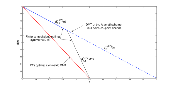
Figure 7: Comparison between the optimal DMT of finite constellations in the symmetric case and the upper bound on the optimal DMT of IC’s, for $M=K=2$ and $N=1$. Note that in the range $0\leq r\leq\frac{1}{3}$ finite constellations achieve the Alamouti performance, whereas IC’s do not. This illustrates that in the multiple-access channel the constellation and the space-time code can not be separated.

IV Attaining the Optimal DMT for $N\geq\left(K+1\right)M-1$

In this section we show that the upper bound on the DMT of the unconstrained multiple-access channel, derived in section III, is achievable for $N\geq\left(K+1\right)M-1$ by a sequence of IC’s in general and lattices in particular. Essentially, we show for $N\geq\left(K+1\right)M-1$ that IC’s attain DMT that equals to $d^{\ast,\left(FC\right)}_{K,M,N}\left(r_{1},\dots,r_{K}\right)=d^{\ast,\left(FC\right)}_{M,N}\left(\max\left(r_{1},\dots,r_{K}\right)\right)$.

We begin by showing in subsection IV-A that simple orthogonal transmission approaches such as time-division multiple-access (TDMA) or code-division multiple-access (CDMA) will result in sub-optimal performance for $N\geq\left(K+1\right)M-1$. Then, we introduce in subsection IV-B the transmission scheme for each user, followed by presentation of the effective channel induced by the transmission scheme in subsection IV-C. We derive in subsection IV-D for each channel realization an upper bound for the error probability of the ML decoder of an ensemble of $K$ IC’s. Finally, in subsection IV-E we average this upper bound over the channel realizations, and show that the optimal DMT is attained for $N\geq\left(K+1\right)M-1$ .

IV-A Orthogonal Transmission is Sub-optimal

In this subsection we show the sub-optimality of transmission methods that create at the receiver orthogonalization between different independent streams, for any channel realization. The advantage of these transmission schemes is their simplicity. By assigning the IC’s or lattices correctly in the space, they enable to consider each stream independently and reduce the decoding problem to the point-to-point scenario. Such an approach is very natural when considering IC’s in general and lattices in particular, as it involves assigning the streams with dimensions or subspaces that remain orthogonal at the receiver for each channel realization. The IC related to a certain stream lies within the assigned subspace. We show for $N\geq\left(K+1\right)M-1$ that such transmission method is sub-optimal as it requires each user to give up too many dimensions to create the orthogonalization.

At the receiver, orthogonal transmission scheme enables each independent stream to lie within a subspace orthogonal to the other streams, for each channel realization. In order for a transmission scheme to fulfil this property, the streams must be assigned with orthogonal subspaces already at the transmitter, i.e., must be assigned with orthogonal subspaces in $\mathbb{C}^{MT}$ assuming there are $T$ channel uses. Hence, orthogonal transmission schemes require the partition of at most $M$ number of dimensions per channel use between all users. On the other hand, $N\geq\left(K+1\right)M-1$ leads to $N\geq K\cdot M$, and so potentially the $K$ users could transmit together up to $KM$ dimensions per channel use, but not orthogonally. The optimal DMT for the symmetric case for $N\geq\left(K+1\right)M-1$ is $d^{\ast,\left(FC\right)}_{M,N}\left(r\right)$. From Corollary 1 and Theorem 4 we know that in the range $M-1\leq r\leq M$ the optimal DMT is obtained only when each user transmits over $M$ average number of dimensions per channel use, i.e., the $K$ users must transmit together $KM$ dimensions per channel use. Hence, orthogonal transmission is not provided with enough dimensions per channel use to obtain the last line of the optimal DMT. This leads to its sub-optimality.

As a first example we consider an orthogonal transmission scheme that takes the natural partition to $K$ streams induced by the multiple-access channel. In order to obtain orthogonalization for this case, at each channel use a different user transmits, while the others wait for their turn to transmit. This transmission method is coined TDMA. Let us consider the symmetric case for which each user transmits at multiplexing gain $r$. For this case, for $T$ channel uses and $K$ users, each user transmits over $\frac{T}{K}$ channel uses. Therefore, each user can achieve the point-to-point performance of a channel with $M$ transmit and $N$ receive antennas, using $\frac{T}{K}$ channel uses. However, in order for each user to transmit at multiplexing gain $r$ per channel use, he must transmit at multiplexing gain $Kr$ over those $\frac{T}{K}$ channel uses, which leads to DMT performance of $d^{\ast,\left(FC\right)}_{M,N}\left(Kr\right)$. This shows the sub-optimality of TDMA.

Another transmission approach is assigning an independent stream for each transmit antenna. This is equivalent to considering a multiple-access channel with $KM$ users, each with a single transmit antenna. Let us consider for example a multiple-access channel with $M=1$, $K$ users and $N\geq K$. In this case the optimal DMT for the symmetric case equals $d^{\ast,\left(FC\right)}_{1,N}\left(r\right)$. On the other hand for CDMA each user is assigned with an orthogonal subspace in $\mathbb{C}^{T}$, assuming there are $T$ channel uses. In this way each stream can obtain the performance of a point-to-point channel with a single transmit antenna and $N$ receive antennas. However, for the orthogonalization to hold each user is assigned with $\frac{T}{K}$ dimensional subspace, which must be orthogonal to the other users subspaces. Hence, in order for each user to obtain multiplexing gain $r$ per channel use, he must transmit at multiplexing gain $Kr$ over the $\frac{T}{K}$ dimensional subspace. This leads to suboptimal DMT performance of $d^{\ast,\left(FC\right)}_{1,N}\left(Kr\right)$.

IV-B The Transmission Scheme

From subsection IV-A we get that an optimal transmission scheme must allow different users to lie in overlapping subspaces at the receiver, i.e., at the receiver the users can not reside in orthogonal subspaces. Essentially, for the proposed transmission scheme each user transmits as if the channel was a point-to-point channel with $M$ transmit and $N$ receive antennas. Hence, each user transmission matrix is identical to the transmission matrix presented in [8].

We denote the transmission matrix of user $i$ by $G_{l}^{\left(i\right)}$, where $l=0,\dots,M-1$ and $i=1,\dots,K$. $G_{l}^{\left(i\right)}$ has $M$ rows that represent the transmission antennas, and $T_{l}=N+M-1-2\cdot l$ columns that represent the number of channel uses. $G_{l}^{\left(i\right)}$ transmits over $D_{l}=\frac{NM-l\left(l+1\right)}{N+M-1-2l}$ average number of dimensions per channel use in the following manner.

Consider a channel with $M$ transmit and $N$ receive antennas.

1. For $D_{M-1}=\frac{M(N-M+1)}{N-M+1}=M$: the matrix $G_{M-1}^{\left(i\right)}$ has $N-M+1$ columns (channel uses). In the first column transmit symbols $x_{1},\dots,x_{M}$ on the $M$ antennas, and in the $N-M+1$ column transmit symbols $x_{M(N-M)+1},\dots,x_{M(N-M+1)}$ on the $M$ antennas.

2. For $D_{l}$, $l=0,\dots,L-2$: the matrix $G_{l}^{\left(i\right)}$ has $M+N-1-2\cdot l$ columns. We add to $G_{l+1}^{\left(i\right)}$, the transmission scheme for $D_{l+1}$, two columns in order to get $G_{l}^{\left(i\right)}$. In the first added column transmit $l+1$ symbols on antennas $1,\dots,l+1$. In the second added column transmit different $l+1$ symbols on antennas $M-l,\dots,M$.

According to the definition of the transmission scheme we can see that the different users transmit the same average number of dimensions per channel use. Let us denote the transmission scheme of the first $k$ users by

$$G_{l}^{\left(1,\dots,k\right)}=\left(G_{l}^{\left(1\right)\dagger},\dots,G_{l}^{\left(k\right)\dagger}\right)^{\dagger}\quad k=1,\dots,K.$$ (10)

$G_{l}^{\left(1,\dots,k\right)}$ is a $k\cdot M\times T_{l}$ matrix. Note that $G_{l}^{\left(1,\dots,k\right)}$ transmits over $k\cdot D_{l}\cdot T_{l}$ dimensions. Later in this section we show that $G_{l}^{\left(1,\dots,K\right)}$ attains the optimal DMT in the range $l\leq r_{max}\leq l+1$.

Example: $M=2$, $N=5$ and $K=2$. In this case the transmission scheme for $D_{0}=\frac{10}{6}$, $D_{1}=\frac{8}{4}$ ($G_{0}^{\left(1.2\right)}$, $G_{1}^{\left(1.2\right)}$ respectively) is as follows:

$$G_{l}^{\left(1,2\right)}=\left(\begin{array}[]{c}G_{l}^{\left(1\right)}\\ G_{l}^{\left(2\right)}\end{array}\right)=\underbrace{\underbrace{\left(\begin{array}[]{ccccc}x_{1}&x_{3}&x_{5}&x_{7}&|\\ x_{2}&x_{4}&x_{6}&x_{8}&|\\ --&--&--&--&|\\ x_{9}&x_{11}&x_{13}&x_{15}&|\\ x_{10}&x_{12}&x_{14}&x_{16}&|\end{array}\right.}_{D_{1}=\frac{8}{4},G_{1}^{\left(1,2\right)}}\left.\begin{array}[]{cc}x_{17}&0\\ 0&x_{18}\\ --&--\\ x_{19}&0\\ 0&x_{20}\end{array}\right)}_{D_{0}=\frac{10}{6},G_{0}^{\left(1,2\right)}}.$$ (11)

IV-C The Effective Channel

Next we define the effective channel matrix induced by the transmission scheme of the first $k$ users $G_{l}^{\left(1,\dots,k\right)}$, where $k=1,\dots,K$. Let us denote the first $k$ users transmission at time instance $t$ by

$$\underline{x}_{t}=\left(\underline{x}_{t}^{\left(1\right)\dagger},\dots,\underline{x}_{t}^{\left(k\right)\dagger}\right)^{\dagger}\quad t=1,\dots,T_{l}.$$

In accordance with the channel model from (1) we get

$$\underline{y}_{t}=H^{\left(1,\dots,k\right)}\cdot\underline{x}_{t}\quad t=1,\dots,T_{l}.$$

where $H^{\left(1,\dots,k\right)}=\left(H^{\left(1\right)},\dots,H^{\left(k\right)}\right)$, is an $N\times k\cdot M$ matrix. The multiplication $H^{\left(1,\dots,k\right)}\cdot G_{l}^{\left(1,\dots,k\right)}$ yields a matrix with $N$ rows and $T_{l}$ columns, for which each column equals to $H^{\left(1,\dots,k\right)}\cdot\underline{x}_{t}$, $t=1\dots T_{l}$. Each user is transmitting $D_{l}\cdot T_{l}$-complex dimensional IC with $D_{l}\cdot T_{l}$-complex symbols, i.e., $G_{l}^{\left(i\right)}$ has exactly $D_{l}\cdot T_{l}$ non-zero values representing the $D_{l}\cdot T_{l}$ complex-dimensional IC within $\mathbb{C}^{MT_{l}}$. Together, the first $k$ users transmit an effective $k\cdot D_{l}\cdot T_{l}$-dimensional complex IC within $\mathbb{C}^{k\cdot MT_{l}}$. For each column of $G_{l}^{\left(1,\dots,k\right)}$, denoted by $\underline{g}_{m}^{\left(k\right)}$, $m=1\dots,T_{l}$, we define the effective channel that $\underline{g}_{m}^{\left(k\right)}$ sees as $\widehat{H}_{m}$. It consists of the columns of $H^{\left(1,\dots,k\right)}$ that correspond to the non-zero entries of $\underline{g}_{m}^{\left(k\right)}$, i.e., $H^{\left(1,\dots,k\right)}\cdot\underline{g}_{m}^{\left(k\right)}=\widehat{H}_{m}\cdot\underline{\widehat{g}}_{m}^{\left(k\right)}$, where $\underline{\widehat{g}}_{m}^{\left(k\right)}$ equals to the non-zero entries of $\underline{g}_{m}^{\left(k\right)}$. As an example assume without loss of generality that only the first $l_{m}$ entries of $\underline{g}_{m}^{\left(k\right)}$ are not zero. In this case $\widehat{H}_{m}$ is an $N\times l_{m}$ matrix that equals to the first $l_{m}$ columns of $H^{\left(1,\dots,k\right)}$. In accordance with (3), $H_{\mathrm{eff}}^{(l),k}$ is an $NT_{l}\times kD_{l}\cdot T_{l}$ block diagonal matrix consisting of $T_{l}$ blocks. Since each block in $H_{\mathrm{eff}}^{(l),k}$ corresponds to the multiplication of $H^{\left(1,\dots,k\right)}$ with different column in $G_{l}^{\left(1,\dots,k\right)}$, the blocks of $H_{\mathrm{eff}}^{(l),k}$ equal $\widehat{H}_{m}$, $m=1,\dots,T_{l}$. Note that in the effective matrix $NT_{l}\geq k\cdot D_{l}\cdot T_{l}$.

Next we elaborate on the structure of the blocks of $H_{\mathrm{eff}}^{(l),k}$. For this reason we denote the m’th column of $H^{\left(1,\dots,k\right)}$ by $\underline{h}_{m}$, $m=1,\dots,k\cdot M$. The transmission scheme has $N+M-1-2\cdot l$ columns. The entries of the first $N-M+1$ columns of $G_{l}^{\left(1,\dots,k\right)}$, $\underline{g}_{1}^{\left(k\right)},\dots,\underline{g}_{N-M+1}^{\left(k\right)}$ are all different from zero. Hence, the first $N-M+1$ blocks of $H_{\mathrm{eff}}^{(l),k}$ are

$$\widehat{H}_{m}=H^{\left(1,\dots,k\right)}\qquad m=1,\cdots,N-M+1.$$ (12)

After the first $N-M+1$ columns we have $M-1-l$ pairs of columns. For each pair we have

$$\widehat{H}_{N-M+2v}=\widehat{H}_{N-M+2\left(v-1\right)} \setminus\left\{\underline{h}_{M-\left(v-1\right)},\underline{h}_{2M-\left(v-1\right)},\dots,\underline{h}_{kM-\left(v-1\right)}\right\}$$

$$=\{\underline{h}_{1},\dots,\underline{h}_{M-v},\underline{h}_{M+1},\dots,\underline{h}_{2M-v},\dots,\underline{h}_{\left(k-1\right)M+1},\dots,\underline{h}_{k\cdot M-v}\}$$ (13)

and

$$\widehat{H}_{N-M+2v+1}=\widehat{H}_{N-M+2\left(v-1\right)+1} \setminus\left\{\underline{h}_{v},\underline{h}_{v+M},\dots,\underline{h}_{v+kM}\right\}$$

$$=\{\underline{h}_{v+1},\dots,\underline{h}_{M},\underline{h}_{M+v+1},\dots,\underline{h}_{2M},\dots,\underline{h}_{\left(k-1\right)M+v+1},\dots,\underline{h}_{k\cdot M}\}$$ (14)

where $v=1,\dots,M-1-l$.

Example: consider $M=2$, $N=5$ and $K=2$ as presented in (11). In this case $l=0,1$ and we have $D_{0}=\frac{10}{6}$ and $D_{1}=\frac{8}{4}=2$ respectively. In addition $H^{\left(1,2\right)}=\left(H^{\left(1\right)},H^{\left(2\right)}\right)=\left(\underline{h}_{1},\underline{h}_{2},\underline{h}_{3},\underline{h}_{4}\right)$. We begin with $k=1$. In this case we get a point-to-point channel with $2$ transmit and 5 receive antennas $H^{\left(1\right)}=\left(\underline{h}_{1},\underline{h}_{2}\right)$, which leads to the following effective channels

1. $D_{1}=2$: $H_{\mathrm{eff}}^{(l=1),k=1}$ is generated from the multiplication of the $5\times 2$ matrix $H^{\left(1\right)}$ with the four columns of the transmission matrix $G_{1}^{\left(1\right)}$. In this case $H_{\mathrm{eff}}^{(1),1}$ is a $20\times 8$ block diagonal matrix, consisting of four blocks, where each block equals to $H^{\left(1\right)}$.

2. $D_{0}=\frac{10}{6}$: $H_{\mathrm{eff}}^{(l=0),k=1}$ is a $30\times 10$ block diagonal matrix consisting of six blocks. The first four blocks are equal to $H^{\left(1\right)}$. The additional two blocks (induced by columns 5-6 of $G_{0}^{\left(1\right)}$) are vectors. We get that $\widehat{H}_{5}=\underline{h}_{1}$ and $\widehat{H}_{6}=\underline{h}_{2}$.

For $k=2$ the effective channel induced by $G_{l}^{\left(1,2\right)}$ is as follows.

1. $D_{1}=2$: In this case the effective channel $H_{eff}^{\left(l=1\right),k=2}$ is a $20\times 16$ matrix consisting of four blocks, where each block equals $H^{\left(1,2\right)}=\left(H^{\left(1\right)},H^{\left(2\right)}\right)$.

2. $D_{0}=\frac{10}{6}$: In this case the effective channel $H_{eff}^{\left(l=0\right),k=2}$ is a $30\times 20$ matrix consisting of six blocks. The first four blocks equal to $H^{\left(1,2\right)}$, whereas the other two blocks are $\widehat{H}_{5}=\left(\underline{h}_{1},\underline{h}_{3}\right)$ and $\widehat{H}_{6}=\left(\underline{h}_{2},\underline{h}_{4}\right)$.

We present $H_{\mathrm{eff}}^{(0),2}$ of our example in equation (15).

$$H_{\mathrm{eff}}^{(l=0),k=2}=\left(\begin{array}[]{cccccc}H^{\left(1,2\right)}&\boldsymbol{0}&\boldsymbol{0}&\boldsymbol{0}&\boldsymbol{0}&\boldsymbol{0}\\ \boldsymbol{0}&H^{\left(1,2\right)}&\boldsymbol{0}&\boldsymbol{0}&\boldsymbol{0}&\boldsymbol{0}\\ \boldsymbol{0}&\boldsymbol{0}&H^{\left(1,2\right)}&\boldsymbol{0}&\boldsymbol{0}&\boldsymbol{0}\\ \boldsymbol{0}&\boldsymbol{0}&\boldsymbol{0}&H^{\left(1,2\right)}&\boldsymbol{0}&\boldsymbol{0}\\ \boldsymbol{0}&\boldsymbol{0}&\boldsymbol{0}&\boldsymbol{0}&\left(\underline{h}_{1},\underline{h}_{3}\right)&\boldsymbol{0}\\ \boldsymbol{0}&\boldsymbol{0}&\boldsymbol{0}&\boldsymbol{0}&\boldsymbol{0}&\left(\underline{h}_{2},\underline{h}_{4}\right)\end{array}\right)$$ (15)

Now let us consider the rows of $G_{l}^{\left(1,\dots,k\right)}$. Each row of the transmission matrix is related to the column of $H^{\left(1,\dots,k\right)}$ that multiplies it, i.e., row $j$ in $G_{l}^{\left(1,\dots,k\right)}$ corresponds to column $\underline{h}_{j}$. In case there is a non zero entry of row $j$ in column $m$ of $G_{l}^{\left(1,\dots,k\right)}$, it means that $\underline{h}_{j}$ occurs in $\widehat{H}_{m}$. In the next lemma we examine the number of occurrences of a certain column of $H^{\left(1,\dots,k\right)}$ in the blocks of $H_{eff}^{\left(l\right),k}$.

Lemma 7.

For any $k=1,\dots,K$ consider column $\underline{h}_{a\cdot M+b}$ in $H^{\left(1,\dots,k\right)}$, where $a=0,\dots,k-1$ and $b=1,\dots,M$. In this case $\underline{h}_{a\cdot M+b}$ occurs only in the first $m=N-M+1+\min\left(M-l-1,M-b\right)+\min\left(M-l-1,b-1\right)$ blocks of $H_{eff}^{\left(l\right),k}$.

Proof.

Straight forward from the definition of the blocks of $H_{eff}^{\left(l\right),k}$ in (12), (IV-C) and (IV-C). ∎

IV-D Upper Bound on the Error Probability

In this subsection we derive for each channel realization an upper bound for the error probability of the joint ML decoder of $K$ ensembles of IC’s transmitted on the unconstrained multiple-access channel, assuming each IC is $D_{l}\cdot T_{l}$-complex dimensional.

In accordance with the definitions in IV-C we denote the effective channel of any set of users pulled together by $H_{eff}^{\left(l\right),\left(s\right)}$, where $s\subseteq\left\{1,\dots,K\right\}$. We define $|H_{\mathrm{eff}}^{(l),\left(s\right)\dagger}\cdot H_{\mathrm{eff}}^{(l),\left(s\right)}|=\rho^{-\sum_{i=1}^{|s|\cdot D_{l}\cdot T_{l}}\eta_{i}^{\left(s\right)}}$ , where $\rho^{-\frac{\eta_{i}^{\left(s\right)}}{2}}$ is the i’th singular value of $H_{\mathrm{eff}}^{(l),\left(s\right)}$, $1\leq i\leq|s|\cdot D_{l}\cdot T_{l}$. We also define $\underline{\eta}^{\left(s\right)}=(\eta_{1}^{\left(s\right)},\dots,\eta_{|s|\cdot D_{l}\cdot T_{l}}^{\left(s\right)})^{T}$. Note that in our setting $NT_{l}\geq K\cdot D_{l}\cdot T_{l}$.

Theorem 6.

Consider $K$ ensembles of $D_{l}\cdot T_{l}$-complex dimensional IC’s transmitted on the unconstrained multiple-access channel with effective channel $H_{eff}^{\left(l\right),K}$ and densities $\gamma_{tr}^{\left(i\right)}=\rho^{T_{l}r_{i}}$, $i=1,\dots,K$. The average decoding error probability of the joint ML decoder is upper bounded by

$$\overline{Pe}(H_{\mathrm{eff}}^{(l),K},\rho)\leq\sum_{s\subseteq\left\{1,\dots,K\right\}}\overline{Pe}(\underline{\eta}^{\left(s\right)},\rho)=\sum_{s\subseteq\left\{1,\dots,K\right\}}D(|s|\cdot D_{l}\cdot T_{l})\rho^{-\cdot T_{l}(|s|D_{l}-\sum_{i\in s}r_{i})+\sum_{i=1}^{|s|\cdot D_{l}\cdot T_{l}}\eta_{i}^{\left(s\right)}}$$

$$=\sum_{s\subseteq\left\{1,\dots,K\right\}}D(|s|\cdot D_{l}\cdot T_{l})\rho^{-T_{l}(|s|D_{l}-\sum_{i\in s}r_{i})}\cdot|H_{\mathrm{eff}}^{(l),\left(s\right)\dagger}\cdot H_{\mathrm{eff}}^{(l),\left(s\right)}|^{-1}$$

where $D(|s|\cdot D_{l}\cdot T_{l})$ is a constant independent of $\rho$, and $\eta_{i}^{\left(s\right)}\geq 0$ for any $s\subseteq\left\{1,\dots,K\right\}$ and any $1\leq i\leq|s|\cdot D_{l}\cdot T_{l}$.

Proof.

The proof is based on dividing the error event into events of error for different sets of users (disjoint events). Then we show that the upper bound on the error probability for the point-to-point channel derived in [8] can be used to upper bound the probability for each of these events. The full proof is in appendix I. ∎

We wish to emphasize that the constraint of $\eta_{i}^{\left(s\right)}\geq 0$, for $i=1,\dots,|s|\cdot D_{l}\cdot T_{l}$ and for any $s\subseteq\left\{1,\dots,K\right\}$ results from the fact that the same ensemble is upper bounded for any channel realization. In cases where it is possible to fit an ensemble to each channel realization, i.e., in the case where the transmitter knows the channel, the upper bound applies also without this restriction.

IV-E Achieving the Optimal DMT

In this subsection we show that the transmission scheme proposed in IV-B attains the optimal DMT for $N\geq\left(K+1\right)M-1$, $d^{\ast,\left(FC\right)}_{M,N}\left(\max\left(r_{1},\dots,r_{K}\right)\right)$. We base the proof on the upper bound for the error probability derived in Theorem 6. This upper bound consists of the sum of several terms, one for each $s\subseteq\left\{1,\dots,K\right\}$. Each term depends on the determinant corresponding to its effective channel $|H_{eff}^{\left(l\right),\left(s\right)\dagger}\cdot H_{eff}^{\left(l\right),\left(s\right)}|^{-1}$. For each term (for each $s$) we upper bound this determinant in Lemma 8 (different bounds than the bounds used in [8]) to get a new upper bound on the error probability. The upper bound is based on the fact that a determinant equals to the multiplication of the orthogonal elements of its columns (when the number of rows is larger than the number of columns). We average the upper bound over the channel realizations and show it attains the optimal DMT in Theorem 7, and also prove that the results apply to lattices when regular lattice decoder is employed at the receiver, in Theorem 8.

Each term in the upper bound in Theorem 6 can be viewed as the error probability of a point-to-point channel with $|s|\cdot M$ transmit antennas and $N$ receive antennas, while transmitting an $|s|\cdot D_{l}\cdot T_{l}$-complex dimensional IC in the method described in IV-B. We wish to emphasize that in this subsection we show that the terms corresponding to $|s|=1$ attain the required optimal DMT since each user uses an optimal transmission scheme for the point-to-point channel with $M$ transmit and $N$ receive antennas. However, for the terms corresponding to $1<|s|\leq K$ the effective transmission scheme is no longer optimal and does not necessarily attain the optimal DMT for a point-to-point channel with $|s|\cdot M$ transmit and $N$ receive antennas. In fact it does not even necessarily attain $d^{\ast,|s|\cdot D_{l}}_{|s|\cdot M,N}\left(\max\left(r_{1},\dots,r_{K}\right)\right)$. Hence, the challenge in this subsection is to upper bound the DMT of these terms and show that, although not optimal for the corresponding point-to-point channel, they attain the optimal DMT of the multiple-access channel for $N\geq\left(K+1\right)M-1$.

The average decoding error probability equals to the average over all channel realizations, i.e.,

$$\overline{Pe}(\rho)=E_{H}\left(\overline{Pe}\left(H_{\mathrm{eff}}^{(l),K},\rho\right)\right).$$ (16)

Based on Theorem 6 we get the following upper bound on the average decoding error probability

$$\overline{Pe}(\rho)\leq\sum_{s\subseteq\left\{1,\dots,K\right\}}E_{H}\left(D(|s|\cdot D_{l}\cdot T_{l})\rho^{-T_{l}(|s|D_{l}-\sum_{i\in s}r_{i})}\cdot|H_{\mathrm{eff}}^{(l),\left(s\right)\dagger}\cdot H_{\mathrm{eff}}^{(l),\left(s\right)}|^{-1}\right).$$ (17)

Note that $E_{H}\left(|H_{\mathrm{eff}}^{(l),\left(s\right)\dagger}H_{\mathrm{eff}}^{(l),\left(s\right)}|^{-1}\right)=E_{H}\left(|H_{\mathrm{eff}}^{(l),|s|\dagger}H_{\mathrm{eff}}^{(l),|s|}|^{-1}\right)$ for any $|s|=k$, where $k=1,\dots,K$, i.e., the mean value for any the users equals to the mean value for the first $k$ users. Therefore, by replacing $H_{\mathrm{eff}}^{(l),\left(s\right)}$ with $H_{\mathrm{eff}}^{(l),|s|}$ we can write (17) as follows

$$\overline{Pe}(\rho)\leq\sum_{s\subseteq\left\{1,\dots,K\right\}}D(|s|\cdot D_{l}\cdot T_{l})\rho^{-T_{l}(|s|D_{l}-\sum_{i\in s}r_{i})}\cdot E_{H}\left(|H_{\mathrm{eff}}^{(l),|s|\dagger}\cdot H_{\mathrm{eff}}^{(l),|s|}|^{-1}\right).$$ (18)

where $H_{\mathrm{eff}}^{(l),|s|}$ is the effective channel of the first $|s|$ users, as defined in subsection IV-C.

The channel matrix $H$ consists of $N\cdot K\cdot M$ i.i.d entries, where each entry has distribution $h_{i,j}\sim\mathcal{CN}(0,1)$, $1\leq i\leq N$ and $1\leq j\leq K\cdot M$. Without loss of generality we consider the case where the columns of $H$ are drawn sequentially from left to right, i.e., $\underline{h}_{1}$ is drawn first, then $\underline{h}_{2}$ is drawn et cetera. Column $\underline{h}_{j}$ is an $N$-dimensional vector. Given $\underline{h}_{1},\dots,\underline{h}_{j-1}$, let us denote by $\underline{\widetilde{h}}_{j}\in\mathbb{C}^{N}$ the elements of the projection of $\underline{h}_{j}$ on an orthonormal basis that depends on $\underline{h}_{1},\dots,\underline{h}_{j-1}$. We can write

$$\underline{h}_{j}=\Theta(\underline{h}_{1},\dots,\underline{h}_{j-1})\cdot\underline{\widetilde{h}}_{j}$$ (19)

where $\Theta(\cdot)$ is an $N\times N$ unitary matrix. $\Theta(\cdot)$ is chosen such that:

1. The first element of $\underline{\widetilde{h}}_{j}$, $\widetilde{h}_{1,j}$, is in the direction of $\underline{h}_{j-1}$.

2. The second element, $\widetilde{h}_{2,j}$, is in the direction orthogonal to $\underline{h}_{j-1}$, in the hyperplane spanned by $\{\underline{h}_{j-1},\underline{h}_{j-2}\}$.

3. Element $\widetilde{h}_{j-1,j}$ is in the direction orthogonal to the hyperplane spanned by $\{\underline{h}_{2},\dots,\underline{h}_{j-1}\}$ inside the hyperplane spanned by $\{\underline{h}_{1},\dots,\underline{h}_{j-1}\}$.

4. The rest of the $N-j+1$ elements are in directions orthogonal to the hyperplane $\{\underline{h}_{1},\dots,\underline{h}_{j-1}\}$.

Note that $\widetilde{h}_{i,j}$, $1\leq i\leq N$, $1\leq j\leq K\cdot M$ are i.i.d random variables with distribution $\mathcal{CN}(0,1)$. Let us denote by $\underline{h}_{j\perp j-1,\dots,j-k}$ the component of $\underline{h}_{j}$ which resides in the $N-k$ subspace which is perpendicular to the space spanned by $\{\underline{h}_{j-1},\dots,\underline{h}_{j-k}\}$. In this case we get

$$\lVert\underline{h}_{j\perp j-1,\dots,j-k}\rVert^{2}=\sum_{i=k+1}^{N}|\widetilde{h}_{i,j}|^{2}\quad 1\leq k\leq j-1.$$ (20)

If we assign $|\widetilde{h}_{i,j}|^{2}=\rho^{-\xi_{i,j}}$, we get that the probability density function (PDF) of $\xi_{i,f}$ is

$$f(\xi_{i,j})=C\cdot\log{\rho}\cdot\rho^{-\xi_{i,j}}\cdot e^{-\rho^{-\xi_{i,j}}}$$ (21)

where $C$ is a normalization factor. In our analysis we assume a very large value for $\rho$. Hence, we can neglect events in which $\xi_{i,j}<0$ since in this case the PDF (21) decreases exponentially as a function of $\rho$. For a very large $\rho$, $\xi_{i,j}\geq 0$, $1\leq i\leq N$ and $1\leq j\leq K\cdot M$, the PDF takes the following form

$$f(\xi_{i,j})\propto\rho^{-\xi_{i,j}}\qquad\xi_{i,j}\geq 0.$$ (22)

In this case by assigning in (20) the vector $\underline{\xi}_{j}=(\xi_{1,j},\dots,\xi_{N,j})^{T}$ with PDF which is proportional to $\rho^{-\sum_{i=1}^{N}\xi_{i,j}}$, we get

$$\lVert\underline{h}_{j\perp j-1,\dots,j-k}\rVert^{2}\dot{=}\rho^{-\min_{z\in\{k+1,\dots,N\}}\xi_{z,j}}$$ (23)

where $1\leq k\leq j-1$. In addition

$$\lVert\underline{h}_{j}\rVert^{2}\dot{=}\rho^{-\min_{z\in\{1,\dots,N\}}\xi_{z,j}}.$$ (24)

As presented in (18), in order to calculate the upper bound on the error probability we need to consider only the effective channel of the first $|s|$ users, $1\leq|s|\leq K$. Hence, in order to obtain an upper bound for the error probability we wish to lower bound the determinant $|H_{\mathrm{eff}}^{(l),|s|\dagger}\cdot H_{\mathrm{eff}}^{(l),|s|}|$ by lower bounding the contribution of each column in the channel matrix $H$ to the determinant. The following lemma presents a lower bound on the determinant.

Lemma 8.

$$|H_{\mathrm{eff}}^{(l),|s|\dagger}\cdot H_{\mathrm{eff}}^{(l),|s|}|\dot{\geq}\prod_{a=0}^{|s|-1}\prod_{b=1}^{M}\rho^{-\left(N-M+1+\min\left(M-l-1,M-b\right)\right)\cdot\min_{z\in\left\{aM+b,\dots,N\right\}}\xi_{z,aM+b}}$$

$$\cdot\prod_{b^{{}^{\prime}}=2}^{M}\rho^{-\sum_{i=1}^{\min\left(M-l-1,b^{{}^{\prime}}-1\right)}\min_{z\in\left\{aM+b^{{}^{\prime}}-i,\dots,N\right\}}\xi_{z,aM+b^{{}^{\prime}}}}.$$

Proof.

The proof is in appendix J. Essentially, the term $\left(N-M+1+\min\left(M-l-1,M-b\right)\right)\cdot\min_{z\in\left\{aM+b,\dots,N\right\}}\xi_{z,aM+b}$ indicates that in the lower bound column $\underline{h}_{aM+b}$ occurs $N-M+1+\min\left(M-l-1,M-b\right)$ times with $\underline{h}_{1},\dots,\underline{h}_{aM+b-1}$ to its left. Therefore, only the elements of $\underline{h}_{aM+b}$ which are orthogonal to this set of columns, $\xi_{z,aM+b}$, where $aM+b\leq z\leq N$ contribute to the lower bound.

The term

$${\sum_{i=1}^{\min\left(M-l-1,b^{{}^{\prime}}-1\right)}\cdot\min_{z\in\left\{aM+b^{{}^{\prime}}-i,\dots,N\right\}}\xi_{z,aM+b^{{}^{\prime}}}}$$

indicates that column $\underline{h}_{aM+b^{{}^{\prime}}}$ occurs $\min\left(M-l-1,b^{{}^{\prime}}-1\right)$ times. However, this time we handle the contribution of the orthogonal elements more carefully. For $1\leq i\leq\min\left(M-l-1,b^{{}^{\prime}}-1\right)$ we consider the elements in $\underline{h}_{aM+b^{{}^{\prime}}}$ which are orthogonal to the set of columns $\underline{h}_{1},\dots,\underline{h}_{aM+b^{{}^{\prime}}-i-1}$. ∎

Now we are ready to lower bound the transmission scheme DMT, based on the lower bound on the determinant in Lemma 8. Let us denote the maximal multiplexing gain by $r_{max}=\max\left(1,\dots,K\right)$, and also assume $l=\lfloor r_{max}\rfloor$.

Theorem 7.

Consider $K$ sequences of ensembles of $D_{l}\cdot T_{l}$-complex dimensional IC’s transmitted over the unconstrained multiple-access channel, where each user transmits at multiplexing-gain $r_{i}$ using $G_{\lfloor r_{max}\rfloor}^{\left(i\right)}$, $i=1,\dots,K$. The DMT this transmission scheme attains is lower bounded by $d^{\ast,\left(FC\right)}_{M,N}\left(r_{max}\right)$.

Proof.

We use the upper bound for the error probability derived in Theorem 6, and the lower bound on the determinant (J) in order to give a new upper bound on the error probability. We average this upper bound over the channel realization, and show that for large $\rho$ the diversity order of the most dominant error event is lower bounded by $d^{\ast,\left(FC\right)}_{M,N}\left(r_{max}\right)$. The full proof is in appendix K. ∎

In Theorem 5 we have shown that for $N\geq\left(K+1\right)M-1$ the DMT of any IC is upper bounded by $d^{\ast,\left(FC\right)}_{M,N}\left(r_{max}\right)$. On the other hand in Theorem 7 we have shown that there exist sequences of IC’s that attain DMT which is lower bounded by $d^{\ast,\left(FC\right)}_{M,N}\left(r_{max}\right)$. Hence, the transmission scheme must attain the optimal DMT.

In the next theorem we prove the existence of a sequence of lattices that attains the optimal DMT as in Theorem 7.

Theorem 8.

For each tuple of multiplexing gains $\left(r_{1},\dots,r_{K}\right)$ there exist $K$ sequences of $2D_{l}\cdot T_{l}$-real dimensional lattices transmitted over the unconstrained multiple access channel that attain diversity order of $d^{\ast,\left(FC\right)}_{M,N}\left(r_{max}\right)$, when regular lattice decoder is employed, where $l=\lfloor r_{max}\rfloor$.

Proof.

See appendix N ∎

Now we show that for each segment of the optimal DMT there exists a sequence of $K$ lattices that attains it, i.e., the optimal DMT consists of $M$ segments, each in the range $l\leq r_{max}\leq l+1$ for $l=0,\dots,M-1$, and there are $M$ sequences of lattices that attain it.

Corollary 3.

For $N\geq\left(K+1\right)M-1$ each segment of the optimal DMT for the unconstrained multiple-access channel, $d^{\ast,\left(FC\right)}_{M,N}\left(r_{max}\right)$, is attained by a sequence of $K$, $2D_{\lfloor r_{max}\rfloor}T_{\lfloor r_{max}\rfloor}$-real dimensional lattices.

Proof.

See appendix O. ∎

IV-F The Gap from the Upper Bound for $N<\left(K+1\right)M-1$

In section III we presented an upper bound on the optimal DMT of IC’s; We showed that when $N<\left(K+1\right)M-1$ IC’s can not achieve the optimal DMT of finite constellations. However, a question that remains open is how tight is the upper bound in this range. In this subsection we give two examples for the performance of IC’s when $N<\left(K+1\right)M-1$, using the transmission scheme presented in subsection IV-B. From the examples it follows that there are cases in which IC’s achieve the upper bound for the symmetric case; however in general the upper bound is not necessarily tight when $N<\left(K+1\right)M-1$.

As a first example let us consider the case where $N=M=K=2$, for which the upper bound on the optimal DMT of IC’s in the symmetric case is

$$d^{\ast,\left(IC\right)}_{2,2,2}\left(r\right)=4-4r.$$

It can be shown by using the technique we presented in this section, that for the transmission matrix

$$G^{\left(1,2\right)}=\left(\begin{array}[]{cc}x_{1}&0\\ 0&x_{2}\\ x_{3}&0\\ 0&x_{4}\end{array}\right)$$

a random ensemble of IC’s can achieve $d^{\ast,\left(IC\right)}_{2,2,2}\left(r\right)$. Thus, in this setting the upper bound on the DMT of IC’s is tight in the symmetric case.

We now consider the case where $M=K=2$ and $N=4$. In this case the upper bound consists of the following three straight lines

$$d^{\ast,\left(IC\right)}_{2,2,4}\left(r\right)=\left\{\begin{array}[]{cc}8-5r&0\leq r\leq 1\\ 7-4r&1\leq r\leq\frac{3}{2}\\ 4-2r&\frac{3}{2}\leq r\leq 2\end{array}\right.$$

Consider the case where each user uses the optimal transmission scheme for a point-to-point channel with $M=2$ and $N=4$ by using the transmission matrix

$$G^{\left(1,2\right)}_{0}=\left(\begin{array}[]{ccccc}x_{1}&x_{3}&x_{5}&x_{7}&0\\ x_{2}&x_{4}&x_{6}&0&x_{8}\\ x_{9}&x_{11}&x_{13}&x_{15}&0\\ x_{10}&x_{12}&x_{14}&0&x_{16}\end{array}\right)$$

for $0\leq r\leq 1$, and

$$G^{\left(1,2\right)}_{1}=\left(\begin{array}[]{ccc}x_{1}&x_{3}&x_{5}\\ x_{2}&x_{4}&x_{6}\\ x_{7}&x_{9}&x_{11}\\ x_{8}&x_{10}&x_{12}\end{array}\right)$$

when $1\leq r\leq 2$. The DMT of this transmission scheme $\frac{16}{3}-\frac{10}{3}r$ for $0\leq r\leq 1$, and $4-2r$ when $1\leq 1\leq 2$, as shown in Figure 8. Therefore, this transmission scheme DMT coincides with the upper bound only when $\frac{3}{2}\leq r\leq 2$. We wish to emphasize that using this transmission scheme simply provides a lower bound for the optimal DMT of IC’s in this setting, and there may exist other transmission schemes that attain $d^{\ast,\left(IC\right)}_{2,2,4}\left(r\right)$.

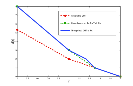
Figure 8: The gap between the upper bound on the DMT of IC’s, and the DMT of the transmission scheme from subsection IV-B, for $M=K=2$ and $N=4$.

In summary, from these examples it follows that when $N<\left(K+1\right)M-1$ the upper bound on the DMT of IC’s is not necessarily tight; nonetheless it enables to show the suboptimality of IC’s in this range.

V Discussion

In this section we discuss the results presented in the paper. As an illustrative example we consider the case in which there are two users, each with two transmit antennas, i.e., $K=M=2$. We consider the symmetric case in which $r_{1}=r_{2}=r$, and explain based on Theorem 4 why for $N=2,4$ IC’s are suboptimal. On the other hand based on Theorem 6 and Theorem 7 we explain why the optimal DMT is attained for $N\geq 5$. The analysis in this section is somewhat loosed and we refer the reader to Sections III, IV for the full analysis.

We begin by giving a short reminder to the behavior of lattices in a point-to-point channel for $M=N=2$, as presented in [8]. We consider in this discussion lattices although the results apply to IC’s in general. In this case, the optimal DMT equals $d^{\ast,\left(FC\right)}_{2,2}\left(r\right)=4-3r$ in the range $0\leq r\leq 1$, and in order to attain it the average number of dimensions per channel use, $D$, must be equal to $\frac{4}{3}$. We wish to explain why for $D\neq\frac{4}{3}$ the optimal DMT is not attained in the range $0\leq r\leq 1$. For lattices, obtaining multiplexing gain $r>0$ requires scaling each dimension of the lattice by $\rho^{-\frac{r}{2D}}$. When $D<\frac{4}{3}$ diversity order of $4$ may be attained for $r=0$. However, the scaling is too strong and does not enable to attain the optimal DMT for any $r>0$ (there are not enough degrees of freedom to attain the straight line $4-3r$). On the other hand when $D>\frac{4}{3}$, the lattice “fills” too much of the space and the channel induces error probability that does not enable to attain diversity order of $4$ for $r=0$, and therefore does not allow attaining the optimal DMT in the range $0\leq r\leq 1$. Hence, choosing $D=\frac{4}{3}$ balances the effect of the scaling and the channel on the lattice and allows to attain the optimal DMT in the range $0\leq r\leq 1$. We now follow this intuition to discuss the multiple-access channel.

V-A Why IC’s are Suboptimal for $N<\left(K+1\right)M-1$

The error event for the multiple-access channel can be divided into the disjoint error events of any subset of the users, as described in Theorem 6. Consider a certain subset of users $s\subseteq\left\{1,\dots,K\right\}$. Due to the distributed nature of the multiple-access channel, the error probability for this subset is upper bounded by the error probability of a point-to-point channel with $|s|\cdot M$ transmit and $N$ receive antennas, i.e., corresponding to a point-to-point channel in which the users in $s$ are pulled together. Hence, the DMT in the multiple-access channel is determined by the most probable error event. For the unconstrained multiple-access channel the problem is more involved as each IC has a certain average number of dimensions per channel use. Assume user $i$ has $D_{i}$ average number of dimensions per channel use, where $1\leq i\leq K$. When considering the error event of users in $s$, we consider an IC with $\sum_{i\in s}D_{i}$ average number of dimensions per channel use. The DMT in this error event is upper bounded by $d^{\ast,\sum_{i\in s}D_{i}}_{|s|\cdot M,N}\left(|s|\cdot r\right)$, i.e., the bounds derived in [8] for the point-to-point channel. In case the dimensions of any subset of the users do not “align”, i.e., in case a certain subset of the users has average number of dimensions per channel use that is too large or too small to attain the optimal DMT, we get sub-optimality. In this subsection we take as example the case $M=K=2$ and explain why for $N=2,4$ the dimensions do not align, and therefore the optimal DMT is not attained.

Let us begin with the case $M=K=N=2$. In this case the optimal DMT in the symmetric case equals

$$d^{\ast,\left(FC\right)}_{K,M,N}\left(r\right)=d^{\ast,\left(FC\right)}_{2,2,2}\left(r\right)=\left\{\begin{array}[]{cc}d^{\ast,\left(FC\right)}_{2,2}\left(r\right)&0\leq r\leq\frac{2}{3}\\ d^{\ast,\left(FC\right)}_{4,2}\left(2r\right)&\frac{2}{3}<r\leq 1\end{array}\right.=\left\{\begin{array}[]{cc}4-3r&0\leq r\leq\frac{2}{3}\\ 6-6r&\frac{2}{3}<r\leq 1\end{array}\right..$$ (25)

On the other hand the optimal DMT of IC’s in this case is upper bounded by $d^{\ast,\left(IC\right)}_{2,2,2}\left(r\right)=4\left(1-r\right)$, which is smaller than the optimal DMT for any $0<r<1$. Let us explain the reason for the sub-optimality. First, note that in the symmetric case we must choose $D_{1}=D_{2}$ to maximize the IC’s DMT, i.e., the users have the same average number of dimensions per channel use. Since $N=2$ each user can not transmit more than one average number of dimensions per channel use, whereas in [8] it was shown that each user needs to transmit $\frac{4}{3}$ average number of dimensions per channel use in order to attain $d^{\ast,\left(FC\right)}_{2,2}\left(r\right)$ in the range $0\leq r\leq\frac{2}{3}$. In addition, the maximal diversity order each user may attain is $4$ since $M=N=2$, and also $d^{\ast,1}_{2,2}\left(r\right)$ is a straight line. Hence, even when transmitting one dimension per channel use the DMT must be smaller than $6-6r$. Therefore, in this case the dimension mismatch manifest itself in the fact that $N$ is too small even to attain the first line of $d^{\ast,\left(FC\right)}_{2,2}\left(r\right)$. This sub-optimality is presented in Figure 3.

For $K=M=2$ and $N=4$ it was shown in Theorem 4 for the symmetric case that IC’s are suboptimal in the range $1<r<\frac{3}{2}$. In this range the DMT of IC’s is upper bounded by $7-4r$, attained at $D_{1}=D_{2}=\frac{7}{4}$. The dimension mismatch manifests itself in this example both in error events of a single user, and the error event of both users. For error events of a single user the optimal DMT is $d^{\ast,\left(FC\right)}_{2,4}\left(r\right)$ which is also the optimal DMT of the multiple-access channel in the range $1\leq r\leq\frac{N}{K+1}=\frac{4}{3}$. The average number of dimensions per channel use required to attain $d^{\ast,\left(FC\right)}_{2,4}\left(r\right)$ for $1\leq r\leq 2$ is $2$ which is larger than $D_{1}=D_{2}=\frac{7}{4}$. Therefore, for the single user error events the scaling of the IC of each user is too strong and does not enable to attain the optimal DMT. On the other hand, for the two users error event the optimal DMT is $d^{\ast,\left(FC\right)}_{4,4}\left(2r\right)$ which is also the optimal DMT in the range $\frac{4}{3}\leq r\leq 2$. The effective IC of the two users pulled together has average number of dimensions per channel use $D_{1}+D_{2}=\frac{7}{2}$, which is too large compared to what is required to attain $d^{\ast,\left(FC\right)}_{2,2}\left(2r\right)$ in the range $1<r<\frac{3}{2}$. Hence, for this error event we get that the effective IC fills too much of the space and so the channel does not enable to attain the optimal DMT.

V-B Why IC’s Attain the Optimal DMT for $N\geq\left(K+1\right)M-1$

For $N\geq\left(K+1\right)M-1$ there is no longer a dimension mismatch. However, the condition that there is no dimension mismatch is merely a necessary condition in order to attain the optimal DMT. Hence, in this subsection we will explain why the optimal DMT is attained based on the transmission scheme presented in subsection IV-B and on the effective channel presented in IV-C.

We consider as an example the case $M=K=2$ and $N=5$. We show why for this case the single user performance $d^{\ast,\left(FC\right)}_{2,5}\left(r_{\max}\right)$ is attained. For simplicity we will focus on the symmetric case. Essentially, we show for this example that IC’s achieve the first DMT line, $10-6r$, which coincides with the optimal DMT $d^{\ast,\left(FC\right)}_{2,5}\left(r\right)$ in the range $0\leq r\leq 1$. The transmission scheme $G_{0}^{\left(1,2\right)}$ is presented in (11). Note that each user uses an optimal transmission scheme for the point-to-point channel with $2$ transmit and $5$ receive antennas. Hence, for the error event of each of the users, the DMT is upper bounded by $10-6r$ which is the optimal DMT in the range $0\leq r\leq 1$. Now, it is left to show for the error event of the two users, that the DMT is also upper bounded by $10-6r$. For this case we consider the effective lattice of the two users pulled together, i.e., an error event for a lattice transmitted over a point-to-point channel with $4$ transmit and $5$ receive antennas. For this lattice the average number of dimensions per channel use equals $D_{1}+D_{2}=\frac{10}{3}$. We will show that at $r=0$ this lattice attains diversity order $10$. This will lead to DMT $10-6r$ since the DMT of a lattice is a straight line, and $D_{1}+D_{2}=\frac{10}{3}$.

At the receiver, the effective radius of the lattice of the two users pulled together at $r=0$ is

$$r_{eff}^{2}\dot{=}|V|^{\frac{1}{\left(D_{1}+D_{2}\right)T}}=\gamma_{\mathrm{rc}}^{-\frac{1}{\left(D_{1}+D_{2}\right)T}}\dot{=}|H_{\mathrm{eff}}^{(l=0),K\dagger}H_{\mathrm{eff}}^{(l=0),K}|^{\frac{1}{\left(D_{1}+D_{2}\right)T}}$$ (26)

where $|V|=\gamma_{\mathrm{rc}}^{-1}$ is the volume of the Voronoi region of the effective lattice at the receiver. Recall that for lattices $r_{\mathrm{eff}}\geq r_{packing}=\frac{d_{\min}^{\left(lattice\right)}}{2}$, where $r_{packing}$ and $d_{\min}^{\left(lattice\right)}$ are the packing radius and the minimal distance of the lattice respectively. We are interested in the event where $r_{\mathrm{eff}}^{2}$ is in the order of the additive noise variance $\rho^{-1}$. In this case $\left(d_{\min}^{\left(lattice\right)}\right)^{2}$ is in the order of the noise variance or worse, and so the error probability does not reduce with $\rho$. In subsection IV-E it is shown that this event is the dominant error event in determining the DMT of the transmission scheme. From (26) we get that $H_{\mathrm{eff}}^{(l=0),K}$ determines the effective radius at the receiver. From (11) and the description of the effective channel in subsection IV-C we get that $H_{\mathrm{eff}}^{(l=0),K}$ is a block diagonal matrix, where $4$ of its blocks equal $H\in\mathbb{C}^{5\times 4}$. For large $\rho$, the most probable error event ($r_{\mathrm{eff}}^{2}\dot{=}\rho^{-1}$) occurs when the determinant of $H$ reduces with $\rho$, and the determinants of the rest of the blocks in $H_{\mathrm{eff}}^{(l=0),K}$ remain constant with $\rho$. Note that if $|H^{\dagger}H|=\rho^{-\alpha}$, then most likely that the smallest singular value of $H$ equals $\rho^{-\alpha}$ and the rest of the singular values remain constant [3]. In this case we get $|H^{\dagger}H|\dot{=}\rho^{-\alpha}$ with a PDF which is proportional to $\rho^{-\left(5-4+1\right)\alpha}=\rho^{-2\alpha}$. By assigning $\left(D_{1}+D_{2}\right)T=20$ and $|H_{\mathrm{eff}}^{(l=0),K\dagger}H_{\mathrm{eff}}^{(l=0),K}|\dot{=}|H^{\dagger}H|^{4}\dot{=}\rho^{-4\alpha}$ in (26) we get that

$$r_{\mathrm{eff}}^{2}\dot{=}|H^{\dagger}H|^{-\frac{4}{20}}\dot{=}\rho^{-\frac{\alpha}{5}}$$ (27)

with a PDF which is proportional to $\rho^{-2\alpha}$. Hence, $r_{\mathrm{eff}}^{2}=\rho^{-1}$ at $\alpha=-5$. Based on subsection IV-E we get for large $\rho$ that this is the most dominant error event, and by assigning $\alpha=5$ we get that it happens with probability $\rho^{-10}$. Therefore, in this case diversity order of $10$ is attained.

For general $N=\left(K+1\right)M-1$ each user uses an optimal transmission scheme for a point-to-point channel with $M$ transmit and $N$ receive antennas. Since the users do not cooperate, at worst we get that $H_{\mathrm{eff}}^{(l=0),K}$ has $N-M+1$ blocks that equal $H\in\mathbb{C}^{N\times K\cdot M}$. For large $\rho$, we get that $|H^{\dagger}H|=\rho^{-\alpha}$ with PDF proportional to $\rho^{-\left(N-K\cdot M+1\right)\alpha}$. For this case $\left(\sum_{i=1}^{K}D_{i}\right)T=K\cdot M\cdot M$ and so we get

$$r_{\mathrm{eff}}^{2}\dot{=}|H^{\dagger}H|^{-\frac{N-M+1}{\left(\sum_{i=1}^{K}D_{i}\right)T}}\dot{=}\rho^{-\frac{\left(N-M+1\right)\alpha}{KMN}}.$$ (28)

Since $N=\left(K+1\right)M-1$, there is a sufficient amount of equations at the receiver to get $N-M+1=K\cdot M$ and $N-K\cdot M+1=M$. Hence, by substituting in (28) we get

$$r_{\mathrm{eff}}^{2}\dot{=}\rho^{-\frac{\alpha}{N}}$$ (29)

with PDF proportional to $\rho^{-\left(N-KM+1\right)\cdot\alpha}=\rho^{-M\cdot\alpha}$. Therefore, at $\alpha=N$ we get that $r_{\mathrm{eff}}^{2}=\rho^{-1}$ with probability $\rho^{-MN}$, which leads to diversity order $MN$ at $r=0$. In addition, $\sum_{i=1}^{K}D_{i}=\frac{KMN}{N-M+1}$ and so the first line of the optimal DMT is attained. Note that we considered the error event for the $K$ users pulled together. For any of the other error events, which considers a subset $s\subseteq\left(1,\dots,K\right)$ of the $K$ users, the diversity order is larger or equal to $MN$ at $r=0$.

In summary, since the users do not cooperate we get at worst $N-M+1$ occurrences of $H$ in the blocks of $H_{\mathrm{eff}}^{(l=0),K}$. However, when $N\geq\left(K+1\right)M-1$ there is a sufficient amount of receive antennas to compensate for the impact of $H$ on $r_{\mathrm{eff}}^{2}$, by decreasing the probability that $H$ has small determinant.

VI Summary and Further Research

This work studies the DMT of the unconstrained multiple-access channel. For $N\geq\left(K+1\right)M-1$ an explicit upper bound on the optimal DMT of IC’s for any multiplexing-gain tuple is presented. The upper bound coincides with the optimal DMT of finite constellations, for the multiple-access channel . A transmission scheme that attains this upper bound is also introduced and analyzed.

In the case $N<\left(K+1\right)M-1$ an upper bound on the optimal DMT of IC’s is derived. For the general case this upper bound remains in the form of a maximization problem. This maximization problem depends on $|s|$, the number of IC’s pulled together for $1\leq|s|\leq K$, and on the average number of dimensions per channel use for each user. On the other hand for finite constellations the maximization depends only on the number of users pulled together. Hence, finding the upper bound on the optimal DMT of IC’s is more involved. In the symmetric case, where all users transmit with the same multiplexing gain, an explicit upper bound on the optimal DMT of IC’s is presented for $N<\left(K+1\right)M-1$. By using this upper bound, it is shown that IC’s are suboptimal compared to finite constellations in this case.

While this work presents a transmission scheme that attains the optimal DMT for $N\geq\left(K+1\right)M-1$, for the case $N<\left(K+1\right)M-1$ the upper bound on the optimal DMT of IC’s is attained only for some cases. For instance whenever $N=1$, orthogonalization attains the optimal DMT of IC’s for the symmetric case. Also for $K=2$, $M=2$ and $N=3$, the transmission scheme presented in this paper attains the upper bound on the optimal DMT of IC’s for the symmetric case. However, finding a transmission scheme that attains the upper bound on the optimal DMT for all $N<\left(K+1\right)M-1$, remains an open problem even for the symmetric case.

Appendix A Proof of Lemma 2

The proof outline is as follows. First we show that for finite constellations, the single user DMT is smaller than the contracted optimal DMT of any number of users (up to $K$) pulled together. Then we use this relation, together with the anchor points presented in Corollary 1 for the upper bound on IC’s DMT, in order to prove the lemma.

Since $K>1$ and $M$ are positive integers, we get for $N\geq\left(K+1\right)M-1$ that $M\leq\frac{N}{i}$, where $1\leq i\leq K$. Hence for any $d^{\ast,i\cdot D}_{i\cdot M,N}\left(i\cdot r\right)$, the range of average number of dimensions per channel use per user is $0\leq D\leq\min\left(M,\frac{N}{i}\right)=M$, where $1\leq i\leq K$.

We begin by showing that $d^{\ast,\left(FC\right)}_{M,N}\left(r\right)$ is smaller or equal to $d^{\ast,\left(FC\right)}_{i\cdot M,N}\left(i\cdot r\right)$ for $2\leq i\leq K$, where $d^{\ast,\left(FC\right)}_{i\cdot M,N}\left(i\cdot r\right)$ is the optimal DMT of finite constellations contracted by $i$, in a point-to-point channel with $i\cdot M$ transmit and $N$ receive antennas. In the case $N>\left(K+1\right)M-1$ we get that $\frac{N}{K+1}\geq M$. Hence we also get that $\frac{N}{i+1}\geq M$ for $1\leq i\leq K$. Hence, from Theorem 3 we can see that

$$d^{\ast,\left(FC\right)}_{M,N}\left(r\right)\leq d^{\ast,\left(FC\right)}_{i\cdot M,N}\left(i\cdot r\right)\quad 2\leq i\leq K$$ (30)

by replacing $K$ with $i$.

For $N=\left(K+1\right)M-1$ we still get that $\frac{N}{i+1}\geq M$ for $1\leq i\leq K-1$, and again based on Theorem 3

$$d^{\ast,\left(FC\right)}_{M,N}\left(r\right)\leq d^{\ast,\left(FC\right)}_{i\cdot M,N}\left(i\cdot r\right)\quad 2\leq i\leq K-1.$$ (31)

For the remaining case of $i=K$, we can see that for $N=\left(K+1\right)M-1$ we get $M-\frac{1}{K}\leq\frac{N}{K+1}\leq M$. Hence we get from Theorem 3

$$d^{\ast,\left(FC\right)}_{M,N}\left(r\right)\leq d^{\ast,\left(FC\right)}_{K\cdot M,N}\left(K\cdot r\right)\quad 0\leq r\leq M-\frac{1}{K}.$$ (32)

For $M-\frac{1}{K}\leq r\leq M$ both $d^{\ast,\left(FC\right)}_{M,N}\left(r\right)$ and $d^{\ast,\left(FC\right)}_{K\cdot M,N}\left(K\cdot r\right)$ are on the last straight line of the piecewise linear functions. By simply assigning $N=\left(K+1\right)M-1$ we get for $M-\frac{1}{K}\leq r\leq M$

$$d^{\ast,\left(FC\right)}_{M,N}\left(r\right)=d^{\ast,\left(FC\right)}_{K\cdot M,N}\left(K\cdot r\right)=KM\left(M-r\right).$$ (33)

From (30)-(33) we get for $N\geq\left(K+1\right)M-1$ and $0\leq r\leq M$ that

$$d^{\ast,\left(FC\right)}_{M,N}\left(r\right)\leq d^{\ast,\left(FC\right)}_{i\cdot M,N}\left(i\cdot r\right)\quad 2\leq i\leq K.$$ (34)

So far we have proved the relation between the contracted optimal DMT of finite constellations with different number of users pulled together. We now use it in order to prove the relation between $d^{\ast,i\cdot D}_{i\cdot M,N}\left(i\cdot r\right)$ for $1\leq i\leq K$. In Corollary 2 it was shown that for $0<D\leq\min\left(M,N\right)$

$$d^{\ast,D}_{M,N}\left(r\right)\leq d^{\ast,\left(FC\right)}_{M,N}\left(r\right)\quad 0\leq r\leq D.$$ (35)

On the other hand from Corollary 1 we can see that

$$d^{\ast,i\cdot D}_{i\cdot M,N}\left(l\right)=d^{\ast,\left(FC\right)}_{i\cdot M,N}\left(l\right)=\left(i\cdot M-l\right)\left(N-l\right)\quad 1\leq i\leq K$$ (36)

at $l=0$ when $0\leq i\cdot D\leq\frac{i\cdot MN}{i\cdot M+N-1}$, and also for $l=1,\dots,i\cdot M-1$ when $\frac{i\cdot MN-l\left(l-1\right)}{i\cdot M+N-1-2\left(l-1\right)}\leq i\cdot D\leq\frac{i\cdot MN-l\left(l+1\right)}{i\cdot M+N-1-2l}$. Hence based on (34)-(36), and the fact that $d^{\ast,i\cdot D}_{i\cdot M,N}\left(i\cdot r\right)$ is a contraction of $d^{\ast,i\cdot D}_{i\cdot M,N}\left(r\right)$ for $2\leq i\leq K$ we get

$$d^{\ast,i\cdot D}_{i\cdot M,N}\left(0\right)\geq d^{\ast,D}_{M,N}\left(0\right)\quad 2\leq i\leq K$$ (37)

for $0\leq D\leq\frac{MN}{i\cdot M+N-1}$, and

$$d^{\ast,i\cdot D}_{i\cdot M,N}\left(l\right)\geq d^{\ast,D}_{M,N}\left(\frac{l}{i}\right)\quad 2\leq i\leq K$$ (38)

for $l=1,\dots,i\cdot M-1$ and $\frac{MN-\frac{l}{i}\left(l-1\right)}{i\cdot M+N-1-2\left(l-1\right)}\leq D\leq\frac{MN-\frac{l}{i}\left(l+1\right)}{i\cdot M+N-1-2l}$. Since $d^{\ast,i\cdot D}_{i\cdot M,N}\left(i\cdot r\right)$, $1\leq i\leq K$, are straight lines as a function of $r$, and also all of these straight lines are equal zero for $r=D$ , i.e., $d^{\ast,i\cdot D}_{i\cdot M,N}\left(i\cdot D\right)=0$ for $1\leq i\leq K$, the inequalities in (37), (38) leads to

$$d^{\ast,D}_{M,N}\left(r\right)\leq d^{\ast,i\cdot D}_{i\cdot M,N}\left(i\cdot r\right)\quad 2\leq i\leq K$$

for any $0\leq D\leq M$ and $0\leq r\leq D$. This concludes the proof.

Appendix B Proof of Lemma 3

First note that $\frac{N}{i+1}\geq\frac{L}{K}$ for $1\leq i\leq K-1$. Hence from Theorem 3 we get that

$$d^{\ast,\left(FC\right)}_{M,N}\left(r\right)\leq d^{\ast,\left(FC\right)}_{i\cdot M,N}\left(i\cdot r\right)\quad 2\leq i\leq K-1$$ (39)

for $0\leq r\leq\frac{L}{K}$. Based on (35), (36), (39) and Corollary 1 we get that

$$d^{\ast,i\cdot D}_{i\cdot M,N}\left(0\right)\geq d^{\ast,D}_{M,N}\left(0\right)\quad 2\leq i\leq K-1$$ (40)

for $0\leq D\leq\frac{MN}{i\cdot M+N-1}$, and

$$d^{\ast,i\cdot D}_{i\cdot M,N}\left(l\right)\geq d^{\ast,D}_{M,N}\left(\frac{l}{i}\right)\quad 2\leq i\leq K-1$$ (41)

for $l=1,\dots,i\cdot M-1$ and $\frac{MN-\frac{l}{i}\left(l-1\right)}{i\cdot M+N-1-2\left(l-1\right)}\leq D\leq\frac{MN-\frac{l}{i}\left(l+1\right)}{i\cdot M+N-1-2l}$. Again, since $d^{\ast,i\cdot D}_{i\cdot M,N}\left(i\cdot r\right)$, $1\leq i\leq K$, are straight lines as a function of $r$, and also all of these straight lines are equal to zero for $r=D$, the inequalities in (40), (41) lead to

$$d^{\ast,D}_{M,N}\left(r\right)\leq d^{\ast,i\cdot D}_{i\cdot M,N}\left(i\cdot r\right)\quad 2\leq i\leq K-1$$

for any $0\leq D\leq\frac{L}{K}$ and $0\leq r\leq D$.

Appendix C Proof of Lemma 4

Since $M\geq 1$ we get for $N<\left(K-1\right)M+1$ that $L=\frac{N}{K}$. Hence we can consider the range $0\leq r\leq\frac{N}{K}$. We begin the proof by showing that for $N<\left(K-1\right)M+1$, $d^{\ast,D}_{M,N}\left(r\right)$ is inferior compared to $d^{\ast,K\cdot D}_{K\cdot M,N}\left(K\cdot r\right)$, for any $0\leq D\leq\frac{N}{K}$. Then we show that the maximization over $d^{\ast,D}_{M,N}\left(r\right)$ yields $M\cdot N-M\cdot K\cdot r$.

We begin by showing that

$$d^{\ast,D}_{M,N}\left(r\right)\leq d^{\ast,K\cdot D}_{K\cdot M,N}\left(K\cdot r\right)\quad 0\leq D\leq\frac{N}{K}$$

for $0\leq r\leq D$. By assigning $D=\frac{N}{K}$ in $d^{\ast,K\cdot D}_{K\cdot M,N}\left(K\cdot r\right)$ we get

$$d^{\ast,N}_{K\cdot M,N}\left(K\cdot r\right)=\left(K\cdot M-N+1\right)\cdot\left(N-Kr\right).$$

Since $N<\left(K-1\right)M+1$ we get

$$d^{\ast,N}_{K\cdot M,N}\left(0\right)=\left(K\cdot M-N+1\right)\cdot N>M\cdot N.$$ (42)

It follows from Corollary 1 that

$$d^{\ast,N}_{K\cdot M,N}\left(0\right)\leq d^{\ast,K\cdot D}_{K\cdot M,N}\left(0\right)\quad 0\leq D\leq\frac{N}{K}$$ (43)

and also

$$d^{\ast,D}_{M,N}\left(0\right)\leq M\cdot N\quad 0\leq D\leq\frac{N}{K}.$$ (44)

Since $d^{\ast,i\cdot D}_{i\cdot M,N}\left(i\cdot r\right)$ $1\leq i\leq K$ are straight lines as a function of $r$, that equal to zero for $r=D$, and also based on (42), (43), (44) and Lemma 3 we get

$$d^{\ast,D}_{M,N}\left(r\right)\leq d^{\ast,i\cdot D}_{i\cdot M,N}\left(i\cdot r\right)\quad 1\leq i\leq K$$ (45)

for any $0\leq D\leq\frac{N}{K}$ and $0\leq r\leq D$. Hence the optimization problem takes the following form

$$\max_{D}\min_{1\leq i\leq K}d^{\ast,i\cdot D}_{i\cdot M,N}\left(i\cdot r\right)=\max_{D}d^{\ast,D}_{M,N}\left(r\right)\quad 0\leq r\leq\frac{N}{K}.$$ (46)

For $N<\left(K-1\right)M+1$ we get that $\frac{N}{K}<\frac{MN}{N+M-1}$. Also, from Corollary 1 we get that $d^{\ast,D}_{M,N}\left(0\right)=M\cdot N$ for $0\leq D\leq\frac{MN}{N+M-1}$. Hence, in the range $0\leq D\leq\frac{N}{K}$ we get a set of straight lines as a function of $r$, $d^{\ast,D}_{M,N}\left(r\right)$, where $d^{\ast,D}_{M,N}\left(0\right)=MN$ and $d^{\ast,D}_{M,N}\left(D\right)=0$. As a result the maximal value for each $r$ is attained for $D=\frac{N}{K}$, and equals

$$\max_{D}d^{\ast,D}_{M,N}\left(r\right)=d^{\ast,\frac{N}{K}}_{M,N}\left(r\right)=MN-KMr\quad 0\leq r\leq\frac{N}{K}.$$ (47)

Appendix D Proof of Lemma 5

The outline of the proof is as follows. We begin by finding the straight line that equals $d^{\ast,\left(FC\right)}_{M,N}\left(\lfloor\frac{l}{2}\rfloor+1\right)$ at $r=\lfloor\frac{l}{2}\rfloor+1$, and also equals $d^{\ast,\left(FC\right)}_{K\cdot M,N}\left(\left(K-1\right)M+\lfloor\frac{l+1}{2}\rfloor\right)$ for $r=\frac{\left(K-1\right)M+\lfloor\frac{l+1}{2}\rfloor}{K}$; it follows from the setting in the lemma that $\lfloor\frac{l}{2}\rfloor+1<\min\left(M,N\right)$ and $\left(K-1\right)M+\lfloor\frac{l+1}{2}\rfloor<\min\left(KM,N\right)$ for $l=0,\dots,2M-3$. Then we show that the average number of dimensions per channel use per user, $D_{l}$, corresponding to this straight line fulfils Corollary 1, i.e., for $d^{\ast,D}_{M,N}\left(r\right)$, $D_{l}$ is in the range of average number of dimensions per channel use that rotate around the anchor point $d^{\ast,\left(FC\right)}_{M,N}\left(\lfloor\frac{l}{2}\rfloor+1\right)$, and also for $d^{\ast,K\cdot D}_{K\cdot M,N}\left(K\cdot r\right)$, $D_{l}$ is in the range of average number of dimensions per channel use that rotate around the anchor point $d^{\ast,\left(FC\right)}_{K\cdot M,N}\left(K\cdot\frac{\left(K-1\right)M+\lfloor\frac{l+1}{2}\rfloor}{K}\right)$. By showing that the straight line fulfils Corollary 1 for both cases, we get that the straight line equals $d^{\ast,D_{l}}_{M,N}\left(r\right)$ and also $d^{\ast,K\cdot D_{l}}_{K\cdot M,N}\left(K\cdot r\right)$.

Let us denote the straight line by

$$d^{\ast}\left(r\right)=MN-\lfloor\frac{l}{2}\rfloor\cdot\left(\lfloor\frac{l}{2}\rfloor+1\right)-2\cdot\left(\lfloor\frac{l}{2}\rfloor+1\right)\cdot\left(\frac{l}{2}-\lfloor\frac{l}{2}\rfloor\right)-\left(N+M-1-l\right)r.$$

First we wish to show that $d^{\ast}\left(\lfloor\frac{l}{2}\rfloor+1\right)=d^{\ast,\left(FC\right)}_{M,N}\left(\lfloor\frac{l}{2}\rfloor+1\right)$, and also that $d^{\ast}\left(\frac{\left(K-1\right)M+\lfloor\frac{l+1}{2}\rfloor}{K}\right)=d^{\ast,\left(FC\right)}_{K\cdot M,N}\left(\left(K-1\right)M+\lfloor\frac{l+1}{2}\rfloor\right)$. By simply assigning $r=\lfloor\frac{l}{2}\rfloor+1$ we get

$$d^{\ast}\left(\lfloor\frac{l}{2}\rfloor+1\right)=\left(N-\lfloor\frac{l}{2}\rfloor-1\right)\cdot\left(M-\lfloor\frac{l}{2}\rfloor-1\right)=d^{\ast,\left(FC\right)}_{M,N}\left(\lfloor\frac{l}{2}\rfloor+1\right).$$ (48)

For $r=\frac{\left(K-1\right)M+\lfloor\frac{l+1}{2}\rfloor}{K}$ we consider two cases. In the first case assume $l=2b$, i.e., $l$ is even. Under this assumption $\lfloor\frac{l+1}{2}\rfloor=\lfloor\frac{l}{2}\rfloor=b$, and so $r=\frac{\left(K-1\right)M+b}{K}$. By assigning $KM=N+M-1-2b$ in $d^{\ast}\left(r\right)$ we get

$$d^{\ast}\left(\frac{\left(K-1\right)M+b}{K}\right)=MN-b\left(b+M+1\right)-\left(K-1\right)M^{2}=\left(N-\left(K-1\right)M-b\right)\cdot\left(M-b\right)=d^{\ast,\left(FC\right)}_{K\cdot M,N}\left(\left(K-1\right)M+b\right).$$

In the second case $l=2b+1$, i.e., $l$ is odd. In this case we get $\lfloor\frac{l+1}{2}\rfloor=b+1$, $\lfloor\frac{l}{2}\rfloor=b$ and $r=\frac{\left(K-1\right)M+b+1}{K}$. By assigning $KM=N+M-2-2b$ in $d^{\ast}\left(r\right)$ we get

$$d^{\ast}\left(\frac{\left(K-1\right)M+b+1}{K}\right)=MN-\left(b+1\right)\cdot\left(b+M+1\right)-\left(K-1\right)M^{2}=d^{\ast,\left(FC\right)}_{K\cdot M,N}\left(\left(K-1\right)M+b+1\right).$$

Hence from both cases we get

$$d^{\ast}\left(\frac{\left(K-1\right)M+\lfloor\frac{l+1}{2}\rfloor}{K}\right)=d^{\ast,\left(FC\right)}_{K\cdot M,N}\left(\left(K-1\right)M+\lfloor\frac{l+1}{2}\rfloor\right).$$ (49)

Now we wish to show that $d^{\ast}\left(r\right)=d^{\ast,D_{l}}_{M,N}\left(r\right)=d^{\ast,K\cdot D_{l}}_{K\cdot M,N}\left(K\cdot r\right)$. We begin by showing that $d^{\ast}\left(r\right)=d^{\ast,D_{l}}_{M,N}\left(r\right)$. First note that

$$d^{\ast}\left(D_{l}\right)=d^{\ast,D_{l}}_{M,N}\left(D_{l}\right)=d^{\ast,K\cdot D_{l}}_{K\cdot M,N}\left(K\cdot D_{l}\right)=0.$$ (50)

Now let us denote $D_{\lfloor\frac{l}{2}\rfloor}^{\ast}=\frac{M\cdot N-\lfloor\frac{l}{2}\rfloor\cdot\left(\lfloor\frac{l}{2}\rfloor+1\right)}{N+M-1-2\lfloor\frac{l}{2}\rfloor}$ and $D_{\lfloor\frac{l}{2}\rfloor+1}^{\ast}=\frac{M\cdot N-\left(\lfloor\frac{l}{2}\rfloor+1\right)\cdot\left(\lfloor\frac{l}{2}\rfloor+2\right)}{N+M-1-2\left(\lfloor\frac{l}{2}\rfloor+1\right)}$; note that $D_{\lfloor\frac{l}{2}\rfloor+1}^{\ast}>D_{\lfloor\frac{l}{2}\rfloor}^{\ast}$. We wish to show that

$$d^{\ast,D_{\lfloor\frac{l}{2}\rfloor+1}^{\ast}}_{M,N}\left(0\right)=M\cdot N-\left(\lfloor\frac{l}{2}\rfloor+1\right)\cdot\left(\lfloor\frac{l}{2}\rfloor+2\right)<d^{\ast}\left(0\right)\leq M\cdot N-\lfloor\frac{l}{2}\rfloor\cdot\left(\lfloor\frac{l}{2}\rfloor+1\right)=d^{\ast,D_{\lfloor\frac{l}{2}\rfloor}^{\ast}}_{M,N}\left(0\right).$$ (51)

In the first case we take $l=2b$. In this case

$$d^{\ast}\left(0\right)=M\cdot N-b\left(b+1\right).$$

On the other hand we also get

$$M\cdot N-\lfloor\frac{l}{2}\rfloor\cdot\left(\lfloor\frac{l}{2}\rfloor+1\right)=M\cdot N-b\cdot\left(b+1\right)=d^{\ast}\left(0\right)$$

which proves (51) for the first case. In the second case we consider $l=2b+1$. In this case

$$d^{\ast}\left(0\right)=M\cdot N-\left(b+1\right)^{2}.$$

For this case we also get $M\cdot N-\lfloor\frac{l}{2}\rfloor\cdot\left(\lfloor\frac{l}{2}\rfloor+1\right)=M\cdot N-b\cdot\left(b+1\right)$ and $M\cdot N-\left(\lfloor\frac{l}{2}\rfloor+1\right)\cdot\left(\lfloor\frac{l}{2}\rfloor+2\right)=M\cdot N-\left(b+1\right)\cdot\left(b+2\right)$. It can be easily shown that for $b\geq 0$

$$M\cdot N-\left(b+1\right)\cdot\left(b+2\right)<d^{\ast}\left(0\right)=M\cdot N-\left(b+1\right)^{2}\leq M\cdot N-b\cdot\left(b+1\right)$$

which proves (51) for the second case. From Corollary 1 and (48) we know that

$$d^{\ast}\left(\lfloor\frac{l}{2}\rfloor+1\right)=d^{\ast,D_{\lfloor\frac{l}{2}\rfloor}^{\ast}}_{M,N}\left(\lfloor\frac{l}{2}\rfloor+1\right)=d^{\ast,D_{\lfloor\frac{l}{2}\rfloor+1}^{\ast}}_{M,N}\left(\lfloor\frac{l}{2}\rfloor+1\right)=d^{\ast,\left(FC\right)}_{M,N}\left(\lfloor\frac{l}{2}\rfloor+1\right)>0.$$ (52)

Since $d^{\ast}\left(r\right)$, $d^{\ast,D_{\lfloor\frac{l}{2}\rfloor}^{\ast}}_{M,N}\left(r\right)$ and $d^{\ast,D_{\lfloor\frac{l}{2}\rfloor+1}^{\ast}}_{M,N}\left(r\right)$ are all straight lines that fulfil (51), (52) we get for $r>\lfloor\frac{l}{2}\rfloor+1$

$$d^{\ast,D_{\lfloor\frac{l}{2}\rfloor}^{\ast}}_{M,N}\left(r\right)\leq d^{\ast}\left(r\right)<d^{\ast,D_{\lfloor\frac{l}{2}\rfloor+1}^{\ast}}_{M,N}\left(r\right),$$ (53)

whereas

$$d^{\ast,D_{\lfloor\frac{l}{2}\rfloor}^{\ast}}_{M,N}\left(D_{\lfloor\frac{l}{2}\rfloor}^{\ast}\right)=d^{\ast}\left(D_{l}\right)=d^{\ast,D_{\lfloor\frac{l}{2}\rfloor+1}^{\ast}}_{M,N}\left(D_{\lfloor\frac{l}{2}\rfloor+1}^{\ast}\right)=0.$$ (54)

Therefore, it follows from (52), (53) and (54) that

$$D_{\lfloor\frac{l}{2}\rfloor}^{\ast}\leq D_{l}<D_{\lfloor\frac{l}{2}\rfloor+1}^{\ast}.$$ (55)

As a result, from Corollary 1 and (55) we get

$$d^{\ast,D_{l}}_{M,N}\left(\lfloor\frac{l}{2}\rfloor+1\right)=d^{\ast,\left(FC\right)}_{M,N}\left(\lfloor\frac{l}{2}\rfloor+1\right).$$ (56)

Since $d^{\ast}\left(r\right)$ and $d^{\ast,D_{l}}_{M,N}\left(r\right)$ are straight lines and based on the equalities in (48), (50) and (56) we get

$$d^{\ast}\left(r\right)=d^{\ast,D_{l}}_{M,N}\left(r\right).$$ (57)

Next we prove $d^{\ast}\left(r\right)=d^{\ast,K\cdot D_{l}}_{K\cdot M,N}\left(K\cdot r\right)$. Let us denote $r_{l}=\frac{\left(K-1\right)M+\lfloor\frac{l+1}{2}\rfloor}{K}$ and $D_{r_{l}}^{\ast}=\frac{MN-\left(K\cdot r_{l}-1\right)r_{l}}{K\cdot M+N-1-2\left(K\cdot r_{l}-1\right)}$. We wish to show

$$d^{\ast,K\cdot D_{r_{l}+\frac{1}{K}}^{\ast}}_{K\cdot M,N}\left(0\right)\leq d^{\ast}\left(0\right)<d^{\ast,K\cdot D_{r_{l}}^{\ast}}_{K\cdot M,N}\left(0\right).$$ (58)

We consider two cases. For the first case we take $l=2\cdot b$. In this case we get $r_{2b}=\frac{\left(K-1\right)M+b}{K}$, $d^{\ast}\left(0\right)=M\cdot N-b\left(b+1\right)$ and $N=\left(K-1\right)M+1+2b$. Hence we get

$$d^{\ast,K\cdot D^{\ast}_{r_{2b}+\frac{1}{K}}}_{K\cdot M,N}\left(0\right)=KMN-\left(\left(K-1\right)M+b\right)\left(N-b\right)=MN-b\left(N-\left(K-1\right)M\right)+b^{2}.$$ (59)

Since $N-\left(K-1\right)M=1+2b$ we get

$$MN-b\left(N-\left(K-1\right)M\right)+b^{2}=MN-b\left(2b+1\right)+b^{2}=MN-b\left(b+1\right).$$ (60)

From (59) and (60) we get $d^{\ast}\left(0\right)=d^{\ast,K\cdot D_{r_{l}+\frac{1}{K}}^{\ast}}_{K\cdot M,N}\left(0\right)$, which proves (58) for the first case. For the second case we take $l=2b+1$. In this case $r_{2b+1}=\frac{\left(K-1\right)M+b+1}{K}$, $d^{\ast}\left(0\right)=MN-\left(b+1\right)^{2}$ and $N=\left(K-1\right)M+2b+2$. For this case we get

$$d^{\ast,K\cdot D^{\ast}_{r_{2b+1}}}_{K\cdot M,N}\left(0\right)=KMN-\left(\left(K-1\right)M+b\right)\left(N-b-1\right)=MN+\left(b+1\right)\left(K-1\right)M-bN+b\left(b+1\right).$$ (61)

Hence according to (58) we need to show

$$MN+\left(b+1\right)\left(K-1\right)M-bN+b\left(b+1\right)>MN-\left(b+1\right)^{2}.$$ (62)

By assigning $\left(K-1\right)M=N-2b-2$ we get from (62) $N>b+1$. Since $0\leq l=2b+1\leq 2M-3$, the maximal value of $b$ is $b=M-2$, which gives for $N=\left(K-1\right)M+2b+l$

$$N>M>M-1\geq b+1.$$

Hence we get

$$d^{\ast}\left(0\right)<d^{\ast,K\cdot D^{\ast}_{r_{2b+1}}}_{K\cdot M,N}\left(0\right)=d^{\ast,K\cdot D^{\ast}_{r_{l}}}_{K\cdot M,N}\left(0\right).$$ (63)

On the other hand we get

$$d^{\ast,D^{\ast}_{r_{2b+1}+\frac{1}{K}}}_{K\cdot M,N}\left(0\right)=KMN-\left(\left(K-1\right)M+1+b\right)\left(N-b\right).$$ (64)

Hence according to (58), (64) we need to show that

$$MN+b\left(K-1\right)M-N\left(b+1\right)+b\left(b+1\right)\leq MN-\left(b+1\right)^{2}$$ (65)

which again leads to $N>b+1$. Hence we get

$$d^{\ast,K\cdot D^{\ast}_{r_{l}+\frac{1}{K}}}_{K\cdot M,N}\left(0\right)=d^{\ast,K\cdot D^{\ast}_{r_{2b+1}+\frac{1}{K}}}_{K\cdot M,N}\left(0\right)\leq d^{\ast}\left(0\right).$$ (66)

From (63) and (66) we get (58) for the second case. Hence we have proved (58). From Corollary 1 and (49) we know that

$$d^{\ast}\left(\frac{\left(K-1\right)M+\lfloor\frac{l+1}{2}\rfloor}{K}\right) =d^{\ast,K\cdot D^{\ast}_{r_{l}+\frac{1}{K}}}_{K\cdot M,N}\left(\left(K-1\right)M+\lfloor\frac{l+1}{2}\rfloor\right)$$

$$=d^{\ast,K\cdot D^{\ast}_{r_{l}}}_{K\cdot M,N}\left(\left(K-1\right)M+\lfloor\frac{l+1}{2}\rfloor\right)=d^{\ast,\left(FC\right)}_{K\cdot M,N}\left(\left(K-1\right)M+\lfloor\frac{l+1}{2}\rfloor\right).$$ (67)

Since $d^{\ast}\left(r\right)$, $d^{\ast,K\cdot D^{\ast}_{r_{l}}}_{K\cdot M,N}\left(K\cdot r\right)$ and $d^{\ast,K\cdot D^{\ast}_{r_{l}+\frac{1}{K}}}_{K\cdot M,N}\left(K\cdot r\right)$ are all straight lines that fulfil (58), (D), we get similarly to (55) that

$$D_{r_{l}}^{\ast}<D_{l}\leq D_{r_{l}+\frac{1}{K}}^{\ast}.$$ (68)

As a result, from Corollary 1 and (68) we get

$$d^{\ast,K\cdot D_{l}}_{K\cdot M,N}\left(\left(K-1\right)M+\lfloor\frac{l+1}{2}\rfloor\right)=d^{\ast,\left(FC\right)}_{K\cdot M,N}\left(\left(K-1\right)M+\lfloor\frac{l+1}{2}\rfloor\right).$$ (69)

Since $d^{\ast}\left(r\right)$ and $d^{\ast,K\cdot D_{l}}_{K\cdot M,N}\left(K\cdot r\right)$ are straight lines, and based on the equalities in (49), (50) and (69) we get

$$d^{\ast}\left(r\right)=d^{\ast,K\cdot D_{l}}_{K\cdot M,N}\left(K\cdot r\right).$$ (70)

From (57), (70) we get the first part of the Lemma, whereas from (56), (69) we get the second part of the Lemma.

Appendix E Proof of Theorem 4

We begin by showing that $d^{\ast,\left(IC\right)}_{K,M,N}\left(r\right)$ is the solution of the optimization problem in (9), i.e., the case in which all users have the same average number of dimensions per channel use, $D$. Then we show that this is also the solution for (8).

First we find $\max_{D}\,\min_{1\leq i\leq K}\left(d^{\ast,i\cdot D}_{i\cdot M,N}\left(i\cdot r\right)\right)$, where $0\leq r\leq\frac{L}{K}$. In the case $N\geq\left(K+1\right)M-1$, we can see from Lemma 2 that

$$\max_{D}\,\min_{1\leq i\leq K}\left(d^{\ast,i\cdot D}_{i\cdot M,N}\left(i\cdot r\right)\right)=\max_{D}d^{\ast,D}_{M,N}\left(r\right)=d^{\ast,\left(FC\right)}_{M,N}\left(r\right).$$

For $N<\left(K-1\right)M+1$ it was shown in Lemma 4 that $d^{\ast,\left(IC\right)}_{K,M,N}\left(r\right)$ is the optimization problem solution. For $N=\left(K-1\right)M+1+l$ and $l=0,\dots,2M-3$ it follows from Lemma 3 that $d^{\ast,D}_{M,N}\left(r\right)$ is smaller than $d^{\ast,i\cdot D}_{i\cdot M,N}\left(i\cdot r\right)$ for $2\leq i\leq K-1$ and any $0\leq D\leq\frac{L}{K}$, $0\leq r\leq D$. Hence the optimization problem for this case boils down to

$$\max_{D}\,\min\left\{d^{\ast,D}_{M,N}\left(r\right),d^{\ast,K\cdot D}_{K\cdot M,N}\left(K\cdot r\right)\right\}$$ (71)

for $0\leq D\leq\frac{L}{K}$ and $0\leq r\leq D$. From Lemma 5 we know that $d^{\ast,D_{l}}_{M,N}\left(\lfloor\frac{l}{2}\rfloor+1\right)=d^{\ast,\left(FC\right)}_{M,N}\left(\lfloor\frac{l}{2}\rfloor+1\right)$. As a result, based on Corollary 1 we get that for $0<D\leq D_{l}$

$$d^{\ast,D}_{M,N}\left(\lfloor\frac{l}{2}\rfloor+1\right)\leq d^{\ast,\left(FC\right)}_{M,N}\left(\lfloor\frac{l}{2}\rfloor+1\right)=d^{\ast,D_{l}}_{M,N}\left(\lfloor\frac{l}{2}\rfloor+1\right)$$

and also

$$d^{\ast,D}_{M,N}\left(r\right)=0\leq d^{\ast,D_{l}}_{M,N}\left(r\right)\quad r\geq D.$$

Hence we get for $0<D\leq D_{l}$

$$d^{\ast,D}_{M,N}\left(r\right)\leq d^{\ast,D_{l}}_{M,N}\left(r\right)\quad\lfloor\frac{l}{2}\rfloor+1\leq r\leq\frac{L}{K}.$$ (72)

In a similar manner we also know from Lemma 5 that $d^{\ast,K\cdot D_{l}}_{K\cdot M,N}\left(\left(K-1\right)M+\lfloor\frac{l+1}{2}\rfloor\right)=d^{\ast,\left(FC\right)}_{K\cdot M,N}\left(\left(K-1\right)M+\lfloor\frac{l+1}{2}\rfloor\right)$. As a result, based on Corollary 1 we get that for $D_{l}\leq D\leq\frac{L}{K}$

$$d^{\ast,K\cdot D}_{K\cdot M,N}\left(\left(K-1\right)M+\lfloor\frac{l+1}{2}\rfloor\right)\leq d^{\ast,\left(FC\right)}_{K\cdot M,N}\left(\left(K-1\right)M+\lfloor\frac{l+1}{2}\rfloor\right)=d^{\ast,K\cdot D_{l}}_{K\cdot M,N}\left(\left(K-1\right)M+\lfloor\frac{l+1}{2}\rfloor\right)$$

and also

$$d^{\ast,K\cdot D_{l}}_{K\cdot M,N}\left(K\cdot r\right)=0\leq d^{\ast,K\cdot D}_{K\cdot M,N}\left(K\cdot r\right)\quad r\geq D_{l}.$$

Since $D_{l}\geq\frac{\left(K-1\right)M+\lfloor\frac{l+1}{2}\rfloor}{K}$ and these are straight lines, we also get for $D_{l}\leq D\leq\frac{L}{K}$

$$d^{\ast,K\cdot D}_{K\cdot M,N}\left(K\cdot r\right)\leq d^{\ast,K\cdot D_{l}}_{K\cdot M,N}\left(K\cdot r\right)$$ (73)

where $0\leq r\leq\frac{\left(K-1\right)M+\lfloor\frac{l+1}{2}\rfloor}{K}$. Hence, based on (72), (73) and the fact that $d^{\ast,D_{l}}_{M,N}\left(r\right)=d^{\ast,K\cdot D_{l}}_{K\cdot M,N}\left(K\cdot r\right)=d^{\ast}\left(r\right)$ (Lemma 5), we get that

$$\max_{D}\,\min\left\{d^{\ast,D}_{M,N}\left(r\right),d^{\ast,K\cdot D}_{K\cdot M,N}\left(K\cdot r\right)\right\}=d^{\ast}\left(r\right)=d^{\ast,\left(IC\right)}_{K,M,N}\left(r\right)\quad\lfloor\frac{l}{2}\rfloor+1\leq r\leq\frac{\left(K-1\right)M+\lfloor\frac{l+1}{2}\rfloor}{K}.$$ (74)

for $\lfloor\frac{l}{2}\rfloor+1\leq r\leq\frac{\left(K-1\right)M+\lfloor\frac{l+1}{2}\rfloor}{K}$.

We now find the solution for $0\leq r\leq\lfloor\frac{l}{2}\rfloor+1$. Our starting point is $D=D_{l}$ for which $d^{\ast,D_{l}}_{M,N}\left(r\right)=d^{\ast,K\cdot D_{l}}_{K\cdot M,N}\left(K\cdot r\right)$. Since $d^{\ast}\left(\lfloor\frac{l}{2}\rfloor+1\right)=d^{\ast,\left(FC\right)}_{M,N}\left(\lfloor\frac{l}{2}\rfloor+1\right)$ we get from Corollary 1 and (55) that

$$\frac{MN-\lfloor\frac{l}{2}\rfloor\left(\lfloor\frac{l}{2}\rfloor+1\right)}{M+N-1-2\lfloor\frac{l}{2}\rfloor}\leq D_{l}<\frac{MN-\left(\lfloor\frac{l}{2}\rfloor+1\right)\left(\lfloor\frac{l}{2}\rfloor+2\right)}{M+N-1-2\left(\lfloor\frac{l}{2}\rfloor+1\right)}.$$ (75)

It follows from Corollary 2 that for $D_{l}\leq D\leq\frac{L}{K}$

$$d^{\ast,D}_{M,N}\left(r\right)\leq d^{\ast,\left(FC\right)}_{M,N}\left(r\right).$$ (76)

In addition it can be easily shown that for $N=\left(K-1\right)M+1+l$ and $l=0,\dots,2M-3$

$$\lfloor\frac{l}{2}\rfloor+1\leq\frac{N}{K+1}\leq\frac{\left(K-1\right)M+\lfloor\frac{l+1}{2}\rfloor}{K}$$ (77)

by considering the cases in which $l$ is even and odd, i.e., the cases where $l=2b$ and $l=2b+1$. In the case $\frac{MN-\lfloor\frac{l}{2}\rfloor\left(\lfloor\frac{l}{2}\rfloor+1\right)}{M+N-1-2\lfloor\frac{l}{2}\rfloor}\leq D\leq D_{l}$ assume $d^{\ast,K\cdot D}_{K\cdot M,N}\left(K\cdot r\right)$ rotates around anchor point with multiplexing gain $m$. In this case there are two possibilities. The first possibility is $\lfloor\frac{l}{2}\rfloor+2\leq m\leq\frac{L}{K}$ where $m\in\mathbb{Z}$. In this case we get from Corollary 1 that in the range $\frac{MN-\lfloor\frac{l}{2}\rfloor\left(\lfloor\frac{l}{2}\rfloor+1\right)}{M+N-1-2\lfloor\frac{l}{2}\rfloor}\leq D<D_{l}$

$$d^{\ast,D}_{M,N}\left(\lfloor\frac{l}{2}\rfloor+1\right)=d^{\ast,K\cdot D_{l}}_{K\cdot M,N}\left(\lfloor\frac{l}{2}\rfloor+1\right)\leq d^{\ast,K\cdot D}_{K\cdot M,N}\left(\lfloor\frac{l}{2}\rfloor+1\right).$$ (78)

For the second possibility $0\leq m\leq\lfloor\frac{l}{2}\rfloor+1$ we get from (77), Corollary 2 and Theorem 3 that

$$d^{\ast,K\cdot D}_{K\cdot M,N}\left(K\cdot m\right)=d^{\ast,\left(FC\right)}_{K\cdot M,N}\left(K\cdot m\right)\geq d^{\ast,\left(FC\right)}_{M,N}\left(m\right)\geq d^{\ast,D}_{M,N}\left(m\right).$$ (79)

In addition $d^{\ast,D}_{M,N}\left(D\right)=d^{\ast,K\cdot D}_{K\cdot M,N}\left(K\cdot D\right)=0$. Since these are straight lines we get in the range $\frac{MN-\lfloor\frac{l}{2}\rfloor\left(\lfloor\frac{l}{2}\rfloor+1\right)}{M+N-1-2\lfloor\frac{l}{2}\rfloor}\leq D\leq D_{l}$

$$d^{\ast,D}_{M,N}\left(r\right)\leq d^{\ast,K\cdot D}_{K\cdot M,N}\left(K\cdot r\right).$$ (80)

By induction, for $\frac{MN-\left(s-1\right)s}{M+N-1-2\left(s-1\right)}\leq D\leq\frac{MN-s\left(s+1\right)}{M+N-1-2s}$, $s=\lfloor\frac{l}{2}\rfloor,\dots,1$, assuming $d^{\ast,K\cdot D^{\left(s\right)}}_{K\cdot M,N}\left(K\cdot r\right)\geq d^{\ast,D^{\left(s\right)}}_{M,N}\left(r\right)$ at $D^{\left(s\right)}=\frac{MN-s\left(s+1\right)}{M+N-1-2s}$, we get from similar arguments to (77)-(80) that

$$d^{\ast,D}_{M,N}\left(r\right)\leq d^{\ast,K\cdot D}_{K\cdot M,N}\left(K\cdot r\right).$$ (81)

Finally for $0<D\leq\frac{MN}{N+-1}$, from the same arguments as in (81) we also get

$$d^{\ast,D}_{M,N}\left(r\right)\leq d^{\ast,K\cdot D}_{K\cdot M,N}\left(K\cdot r\right).$$ (82)

Hence, from (80), (81) and (82) we get that in the range $0<D\leq D_{l}$

$$\max_{D}\,\min\left\{d^{\ast,D}_{M,N}\left(r\right),d^{\ast,K\cdot D}_{K\cdot M,N}\left(K\cdot r\right)\right\}=\max_{D}d^{\ast,D}_{M,N}\left(r\right).$$ (83)

Since $D_{l}\geq\frac{MN-\lfloor\frac{l}{2}\rfloor\left(\lfloor\frac{l}{2}\rfloor+1\right)}{M+N-1-2\lfloor\frac{l}{2}\rfloor}$ (75), and also from (76), (83) we get based on Corollary 2

$$\max_{D}\,\min\left\{d^{\ast,D}_{M,N}\left(r\right),d^{\ast,K\cdot D}_{K\cdot M,N}\left(K\cdot r\right)\right\}=d^{\ast,\left(FC\right)}_{M,N}\left(r\right)=d^{\ast,\left(IC\right)}_{K,M,N}\left(r\right)\quad 0\leq r\leq\lfloor\frac{l}{2}\rfloor+1.$$ (84)

Now we wish to find $d^{\ast,\left(IC\right)}_{K,M,N}\left(r\right)$ for $\frac{\left(K-1\right)M+\lfloor\frac{l+1}{2}\rfloor}{K}\leq r\leq\frac{L}{K}$. Let us denote $r_{l}=\frac{\left(K-1\right)M+\lfloor\frac{l+1}{2}\rfloor}{K}$. Since

$$d^{\ast,K\cdot D_{l}}_{K\cdot M,N}\left(\left(K-1\right)M+\lfloor\frac{l+1}{2}\rfloor\right)=d^{\ast,\left(FC\right)}_{K\cdot M,N}\left(\left(K-1\right)M+\lfloor\frac{l+1}{2}\rfloor\right)$$

we get (68)

$$\frac{NM-\left(K\cdot r_{l}-1\right)r_{l}}{KM+N-1-2\left(K\cdot r_{l}-1\right)}<D_{l}\leq\frac{NM-r_{l}\left(K\cdot r_{l}+1\right)}{KM+N-1-2\cdot K\cdot r_{l}}.$$ (85)

It follows from Corollary 2 that in the range $0<D\leq D_{l}$

$$d^{\ast,K\cdot D}_{K\cdot M,N}\left(K\cdot r\right)\leq d^{\ast,\left(FC\right)}_{K\cdot M,N}\left(K\cdot r\right).$$ (86)

For $D_{l}<D\leq\frac{NM-\frac{r_{l}}{K}\left(r_{l}+1\right)}{KM+N-1-2r_{l}}$ assume $d^{\ast,D}_{M,N}\left(r\right)$ rotates around anchor point with multiplexing gain $\frac{m}{K}$, where $m\in\mathbb{Z}$. For $0\leq m<\left(K-1\right)M+\lfloor\frac{l+1}{2}\rfloor$, based on Corollary 1 and Lemma 5 we get

$$d^{\ast,D}_{M,N}\left(\frac{\left(K-1\right)M+\lfloor\frac{l+1}{2}\rfloor}{K}\right) \geq d^{\ast,D_{l}}_{M,N}\left(\frac{\left(K-1\right)M+\lfloor\frac{l+1}{2}\rfloor}{K}\right)$$

$$=d^{\ast,\left(FC\right)}_{K\cdot M,N}\left(\left(K-1\right)M+\lfloor\frac{l+1}{2}\rfloor\right)\geq d^{\ast,K\cdot D}_{K\cdot M,N}\left(\left(K-1\right)M+\lfloor\frac{l+1}{2}\rfloor\right).$$ (87)

For $\left(K-1\right)M+\lfloor\frac{l+1}{2}\leq m\leq L$ we get from (77) and Theorem 3 that

$$d^{\ast,D}_{M,N}\left(m\right)=d^{\ast,\left(FC\right)}_{M,N}\left(m\right)\geq d^{\ast,\left(FC\right)}_{K\cdot M,N}\left(K\cdot m\right)\geq d^{\ast,K\cdot D}_{K\cdot M,N}\left(K\cdot m\right).$$ (88)

We also get $d^{\ast,D}_{M,N}\left(D\right)=d^{\ast,K\cdot D}_{K\cdot M,N}\left(K\cdot D\right)=0$. Since these are straight lines, we get for $D_{l}<D\leq\frac{NM-\frac{r_{l}}{K}\left(r_{l}+1\right)}{KM+N-1-2r_{l}}$

$$d^{\ast,D}_{M,N}\left(r\right)\geq d^{\ast,K\cdot D}_{K\cdot M,N}\left(K\cdot r\right).$$ (89)

Similarly to (81) it can be shown by induction for $\frac{MN-\frac{s}{K}\left(s-1\right)}{KM+N-1-2\left(s-1\right)}\leq D\leq\frac{MN-\frac{s}{K}\left(s+1\right)}{KM+N-1-2s}$, $s=\left(K-1\right)M+\lfloor\frac{l+1}{2}\rfloor+1,\dots,L-1$, that

$$d^{\ast,D}_{M,N}\left(r\right)\geq d^{\ast,K\cdot D}_{K\cdot M,N}\left(K\cdot r\right).$$ (90)

Hence, from (86), (89) and (90) we get

$$\max_{D}\,\min\left\{d^{\ast,D}_{M,N}\left(r\right),d^{\ast,K\cdot D}_{K\cdot M,N}\left(K\cdot r\right)\right\}=d^{\ast,\left(FC\right)}_{K\cdot M,N}\left(K\cdot r\right)=d^{\ast,\left(IC\right)}_{K,M,N}\left(r\right)$$ (91)

where $\frac{\left(K-1\right)M+\lfloor\frac{l+1}{2}\rfloor}{K}\leq r\leq\frac{L}{K}$.

The remaining open point for $N=\left(K-1\right)M+1+l$, $l=0,\dots,2M-3$ is the case

$$\lfloor\frac{l}{2}\rfloor+1=\frac{\left(K-1\right)M+\lfloor\frac{l+1}{2}\rfloor}{K}.$$ (92)

First we would like to find when this equality takes place. For this we consider two cases. First let us consider $l=2b$. For this case (92) takes the following form

$$K\cdot\left(b+1\right)=\left(K-1\right)M+b$$

which leads to

$$b=M-\frac{K}{K-1}.$$

Since $b\geq 0$, $M\geq 1$ and $K\geq 2$ are integers, we get that this equality can only hold at $K=2$. In this case we get $M=b+2$ and $N=3\left(b+1\right)$. Since both $M\geq 1$ and $N\geq 1$, we get that $b\geq 2$. Hence by assigning $s=b+1$ we get (92) for $K=2$, $M=s+1$ and $N=3\cdot s$, where $s\geq 1$ is an integer. For the second case we consider $l=2b+1$. In this case by assigning in (92) we get $b=M-1$. However we know that $l=2b+1\leq 2M-3$, and so $b\leq M-2$. Hence for $l=2b+1$ (92) can not take place. From (77), (92) we get

$$\lfloor\frac{l}{2}\rfloor+1=\frac{N}{K+1}=\frac{\left(K-1\right)M+\lfloor\frac{l+1}{2}\rfloor}{K}.$$ (93)

In addition, (92) holds only for $l=2b$. For this case simply by assigning $l=2b$ we get

$$D^{\ast}_{\lfloor\frac{l}{2}\rfloor}=D_{l}=D^{\ast}_{r_{l}}.$$ (94)

Hence, we are interested in finding $d^{\ast,\left(IC\right)}_{K,M,N}\left(r\right)$ for $K=2$, $M=s+1$ and $N=3\cdot s$, where $s\geq 1$ is an integer. For $D>D_{l}$ we get $d^{\ast,D}_{s+1,3\cdot s}\left(r\right)\leq d^{\ast,\left(FC\right)}_{s+1,3\cdot s}\left(r\right)$. On the other hand for $0<D<D_{l}=D^{\ast}_{\lfloor\frac{l}{2}\rfloor}$ we know from Corollary 1 and (93) that $d^{\ast,D}_{s+1,3\cdot s}\left(r\right)$ rotates around anchor point at multiplexing gain $m\leq\frac{N}{K+1}$. Hence, by similar arguments to the ones used in (79) we get $d^{\ast,D}_{s+1,3\cdot s}\left(m\right)\leq d^{\ast,2\cdot D}_{2\cdot\left(s+1\right),3\cdot s}\left(2\cdot m\right)$, which leads to $d^{\ast,D}_{s+1,3\cdot s}\left(r\right)\leq d^{\ast,2\cdot D}_{2\cdot\left(s+1\right),3\cdot s}\left(2\cdot r\right)$ for $0<D<D_{l}$. Hence in the range $0\leq r\leq\frac{N}{K+1}$ the optimal solution is $d^{\ast,\left(FC\right)}_{s+1,3\cdot s}\left(r\right)$. For the same arguments we get for $\frac{N}{K+1}\leq r\leq\frac{L}{K}$ that the optimal solution is $d^{\ast,\left(FC\right)}_{2\cdot\left(s+1\right),3\cdot s}\left(2\cdot r\right)$. Hence we get

$$d^{\ast,\left(IC\right)}_{K,M,N}\left(r\right)=d^{\ast,\left(IC\right)}_{2,s+1,3\cdot s}\left(r\right)=\left\{\begin{array}[]{lr}d^{\ast,\left(FC\right)}_{s+1,3\cdot s}\left(r\right)&0\leq r\leq\frac{N}{K+1}=s\\ d^{\ast,\left(FC\right)}_{2\left(s+1\right),3\cdot s}\left(2\cdot r\right)&s\leq r\leq 3\cdot s.\end{array}\right.$$ (95)

So far we have shown that

$$\max_{D}\,\min\left\{d^{\ast,D}_{M,N}\left(r\right),d^{\ast,K\cdot D}_{K\cdot M,N}\left(K\cdot r\right)\right\}=d^{\ast,\left(IC\right)}_{K,M,N}\left(r\right).$$ (96)

Now we wish to show that this is also the solution of (8). We begin with the case for which $d^{\ast,\left(IC\right)}_{K,M,N}\left(r\right)=d^{\ast,\left(FC\right)}_{M,N}\left(r\right)$. This is the case for $N\geq\left(K+1\right)M-1$, and also for $N=\left(K-1\right)M-1+l$, $l=0,\dots,2M-3$ when $0\leq r\leq\lfloor\frac{l}{2}\rfloor+1$. As a base line we consider the case $D_{1}=\dots,D_{K}=D^{\ast}_{r}$, where $D^{\ast}_{r}$ is the average number of dimensions per channel use per user, that maximizes the expression in (96). Without loss of generality assume user $i$ has $D_{i}\neq D_{r}^{\ast}$. In this case based on (96) and Corollary 2 we get

$$\min_{A\subseteq\left\{1,\dots,K\right\},D_{i}\neq D_{r}^{\ast}}\left(d^{\ast,\sum_{a\in A}D_{a}}_{|A|\cdot M,N}\left(|A|\cdot r\right)\right)\leq d^{\ast,D_{i}}_{M,N}\left(r\right)\leq d^{\ast,\left(FC\right)}_{M,N}\left(r\right)=\max_{D}\,\min\left\{d^{\ast,D}_{M,N}\left(r\right),d^{\ast,K\cdot D}_{K\cdot M,N}\left(K\cdot r\right)\right\}.$$ (97)

Hence the optimal solution must be $d^{\ast,\left(IC\right)}_{K,M,N}\left(r\right)$, attained for $D_{1}=\dots=D_{K}=D_{r}^{\ast}$. We now consider the case in which $d^{\ast,\left(IC\right)}_{K,M,N}\left(r\right)=d^{\ast,\left(FC\right)}_{K\cdot M,N}\left(K\cdot r\right)$, for which $N=\left(K-1\right)M+1+l$, where $l=0,\dots,2M-3$ and $\frac{\left(K-1\right)M+\lfloor\frac{l+1}{2}\rfloor}{K}\leq r\leq\frac{L}{K}$. In this case the optimal solution in (96) for the $K$ users pulled together is attained for $K\cdot D_{r}^{\ast}$. Let us assume that $\sum_{i=1}^{K}D_{i}\neq K\cdot D_{r}^{\ast}$. In this case we get

$$\min_{A\subseteq\left\{1,\dots,K\right\},\sum_{i=1}^{K}D_{i}\neq K\cdot D_{r}^{\ast}}\left(d^{\ast,\sum_{a\in A}D_{a}}_{|A|\cdot M,N}\left(|A|\cdot r\right)\right)\leq d^{\ast,\left(FC\right)}_{K\cdot M,N}\left(K\cdot r\right)=\max_{D}\,\min\left\{d^{\ast,D}_{M,N}\left(r\right),d^{\ast,K\cdot D}_{K\cdot M,N}\left(K\cdot r\right)\right\}.$$ (98)

Hence the optimal solution must be $d^{\ast,\left(IC\right)}_{K,M,N}\left(r\right)$. Now let us consider the case $N<\left(K-1\right)M+1$. In this case the optimal solution in (96) is attained for $D_{r}^{\ast}=\frac{N}{K}$. Without loss of generality assume $D_{i}<\frac{N}{K}$. In this case we get from Corollary 2 that

$$\min_{A\subseteq\left\{1,\dots,K\right\},D_{i}<\frac{N}{K}}\left(d^{\ast,\sum_{a\in A}D_{a}}_{|A|\cdot M,N}\left(|A|\cdot r\right)\right)\leq MN-KMr=\max_{D}\,\min\left\{d^{\ast,D}_{M,N}\left(r\right),d^{\ast,K\cdot D}_{K\cdot M,N}\left(K\cdot r\right)\right\}.$$ (99)

which shows again that $d^{\ast,\left(IC\right)}_{K,M,N}\left(r\right)$ is the solution. Finally we consider the case where $d^{\ast,\left(IC\right)}_{K,M,N}\left(r\right)=d^{\ast}\left(r\right)$, i.e., the case in which $N=\left(K-1\right)M+1+l$, $l=0,\dots,2M-3$ and $\lfloor\frac{l}{2}\rfloor+1\leq r\leq\frac{\left(K-1\right)M+\lfloor\frac{l+1}{2}\rfloor}{K}$. Following Lemma 5 and Corollary 1 we get without loss of generality that when $D_{1}<D_{l}$

$$\min_{A\subseteq\left\{1,\dots,K\right\},D_{1}<D_{l}}\left(d^{\ast,\sum_{a\in A}D_{a}}_{|A|\cdot M,N}\left(|A|\cdot r\right)\right)\leq d^{\ast,D_{1}}_{M,N}\left(r\right)\leq d^{\ast}\left(r\right)=d^{\ast,D_{l}}_{M,N}\left(r\right),$$ (100)

whereas for $\sum_{i=1}^{K}D_{i}>K\cdot D_{l}$

$$\min_{A\subseteq\left\{1,\dots,K\right\},\sum_{i=1}^{K}D_{i}>K\cdot D_{l}}\left(d^{\ast,\sum_{a\in A}D_{a}}_{|A|\cdot M,N}\left(|A|\cdot r\right)\right)\leq d^{\ast,\sum_{i=1}^{K}D_{i}}_{M,N}\left(K\cdot r\right)\leq d^{\ast}\left(r\right)=d^{\ast,K\cdot D_{l}}_{M,N}\left(K\cdot r\right),$$ (101)

which shows that $d^{\ast,\left(IC\right)}_{K,M,N}\left(r\right)$ is the optimal solution. This concludes the proof.

Appendix F Proof of Lemma 6

For $N\geq\left(K+1\right)M-1$ it can be easily shown based on Lemma 2 and Corollary 1 that

$$d^{\ast,\left(FC\right)}_{K,M,N}\left(r\right)=d^{\ast,\left(FC\right)}_{M,N}\left(r\right)=d^{\ast,\left(IC\right)}_{K,M,N}\left(r\right).$$ (102)

For $N<\left(K-1\right)M+1$ we get $\frac{L}{K}=\frac{N}{K}$. It follows from (42), (43), (44) that

$$d^{\ast,D}_{M,N}\left(0\right)<d^{\ast,K\cdot D}_{K\cdot M,N}\left(0\right).$$

In addition, $d^{\ast,D}_{M,N}\left(r\right)$, $d^{\ast,K\cdot D}_{K\cdot M,N}\left(K\cdot r\right)$ are straight lines, and $d^{\ast,D}_{M,N}\left(D\right)=d^{\ast,K\cdot D}_{K\cdot M,N}\left(K\cdot D\right)=0$. As a consequence we get

$$d^{\ast,D}_{M,N}\left(r\right)<d^{\ast,K\cdot D}_{K\cdot M,N}\left(K\cdot r\right)\leq d^{\ast,\left(FC\right)}_{KM,N}\left(K\cdot r\right)\quad 0<D\leq\frac{N}{K}$$ (103)

for $0<r<D$, where the second inequality results from Corollary 2. In addition, since $\frac{N}{K}<\frac{MN}{N+M-1}$, $0<D\leq\frac{N}{K}$ and $\left(N+M-1\right)<K\cdot M$ we get

$$d^{\ast,\left(IC\right)}_{K,M,N}\left(r\right)=MN-KMr<d^{\ast,\left(FC\right)}_{M,N}\left(r\right)=MN-\left(N+M-1\right)r$$ (104)

for $0<r\leq\frac{N}{K}$. Since $d^{\ast,\left(FC\right)}_{K,M,N}\left(r\right)$ consists of $d^{\ast,\left(FC\right)}_{M,N}\left(r\right)$ and $d^{\ast,\left(FC\right)}_{KM,N}\left(K\cdot r\right)$ we get from (103), (104) that

$$d^{\ast,\left(IC\right)}_{K,M,N}\left(r\right)<d^{\ast,\left(FC\right)}_{K,M,N}\left(r\right)\quad 0<r<\frac{N}{K}.$$

For $N=\left(K-1\right)M+1+l$ and $l=0,\dots,2M-3$, recall that we denoted $D_{l}=\frac{MN-\lfloor\frac{l}{2}\rfloor\cdot\left(\lfloor\frac{l}{2}\rfloor+1\right)-2\cdot\left(\lfloor\frac{l}{2}\rfloor+1\right)\cdot\left(\frac{l}{2}-\lfloor\frac{l}{2}\rfloor\right)}{N+M-1-l}$ and also $r_{l}=\frac{\left(K-1\right)M+\lfloor\frac{l+1}{2}\rfloor}{K}$. In (55) it was shown that $D_{l}<\frac{MN-\left(\lfloor\frac{l}{2}\rfloor+1\right)\left(\lfloor\frac{l}{2}\rfloor+2\right)}{M+N-1-2\left(\lfloor\frac{l}{2}\rfloor+1\right)}$; following the behavior of the straight lines around the anchor points as presented in Lemma 5 and Corollary 1, it is straightforward to see that

$$d^{\ast}\left(r\right)=d^{\ast,D_{l}}_{M,N}\left(r\right)<d^{\ast,\left(FC\right)}_{M,N}\left(r\right)\quad\lfloor\frac{l}{2}\rfloor+1<r\leq\frac{L}{K}.$$ (105)

On the other hand from (68) we get $D_{l}>\frac{MN-r_{l}\left(K\cdot r_{l}-1\right)}{K\cdot M+N-1-2\left(\cdot K\cdot r_{l}-1\right)}$. From similar arguments to (105) it follows that

$$d^{\ast}\left(r\right)=d^{\ast,K\cdot D_{l}}_{K\cdot M,N}\left(K\cdot r\right)<d^{\ast,\left(FC\right)}_{K\cdot M,N}\left(K\cdot r\right)$$ (106)

where $0\leq r<\frac{\left(K-1\right)M+\lfloor\frac{l+1}{2}\rfloor}{K}$. Since $d^{\ast,\left(FC\right)}_{K,M,N}\left(r\right)$ consists of $d^{\ast,\left(FC\right)}_{M,N}\left(r\right)$ and $d^{\ast,\left(FC\right)}_{K\cdot M,N}\left(K\cdot r\right)$, we get from (105), (106)

$$d^{\ast}\left(r\right)<d^{\ast,\left(FC\right)}_{K,M,N}\left(r\right)\quad\lfloor\frac{l}{2}\rfloor+1<r<\frac{\left(K-1\right)M+\lfloor\frac{l+1}{2}\rfloor}{K}.$$ (107)

The remaining open point for $N=\left(K-1\right)M+1+l$ and $l=0,\dots,2M-3$ is the case

$$\lfloor\frac{l}{2}\rfloor+1=\frac{\left(K-1\right)M+\lfloor\frac{l+1}{2}\rfloor}{K}.$$

In Theorem 4 it was shown (see equation (93) appendix E) that we get equality for $K=2$, $M=s+1$ and $N=3\cdot s$, where $s\geq 1$ is an integer. According to Theorem 3, for this case the optimal DMT of finite constellations equals

$$d^{\ast,\left(FC\right)}_{2,s+1,3\cdot s}\left(r\right)=\left\{\begin{array}[]{lr}d^{\ast,\left(FC\right)}_{s+1,3\cdot s}\left(r\right)&0\leq r\leq\frac{N}{K+1}=s\\ d^{\ast,\left(FC\right)}_{2\left(s+1\right),3\cdot s}\left(2\cdot r\right)&s\leq r\leq 3\cdot s.\end{array}\right.$$

Hence, from (95) we get $d^{\ast,\left(FC\right)}_{2,s+1,3\cdot s}\left(r\right)=d^{\ast,\left(IC\right)}_{2,s+1,3\cdot s}\left(r\right)$. By simply assigning we get that in this case $N<\left(K+1\right)M-1$. This concludes the proof.

Appendix G Proof of Theorem 5

We begin by finding for $N\geq\left(K+1\right)M-1$ an upper bound on the DMT of the unconstrained multiple-access channel, that equals to the optimal DMT of finite constellations $d^{\ast,\left(FC\right)}_{M,N}\left(\max\left(r_{1},\dots,r_{K}\right)\right)$. The proof relies on the upper bound on the optimal DMT in the symmetric case $d^{\ast,\left(IC\right)}_{K,M,N}\left(r\right)$. For $N\geq\left(K+1\right)M-1$ it was shown in Lemma 6 that

$$d^{\ast,\left(IC\right)}_{K,M,N}\left(r\right)=d^{\ast,\left(FC\right)}_{M,N}\left(r\right).$$ (108)

From Theorem 2 we get that the optimal DMT is upper bounded by

$$\max_{\left(D_{1},\dots,D_{K}\right)\in\mathbf{D}}\min_{A\subseteq\left\{1,\dots,K\right\}}d^{\ast,D_{A}}_{|A|\cdot M,N}\left(R_{A}\right).$$ (109)

We wish to solve (109). We solve it by finding upper and lower bounds on (109) that coincide. For the rate tuple $\left(r_{1},\dots,r_{K}\right)$ recall the definition $r_{max}=\max\left(r_{1},\dots,r_{K}\right)$. We begin by lower bounding the optimization problem terms. Based on Lemma 2 and the fact that $d^{\ast,i\cdot D}_{i\dot{M},N}\left(i\cdot r\right)$, $i=1,\dots,K$ are straight lines as a function of $r$ we get

$$d^{\ast,\sum_{a\in A}D_{a}}_{|A|\cdot M,N}\left(\sum_{a\in A}r_{a}\right)\geq d^{\ast,\sum_{a\in A}D_{a}}_{|A|\cdot M,N}\left(|A|\cdot r_{max}\right)\geq d^{\ast,\frac{\sum_{a\in A}D_{a}}{|A|}}_{M,N}\left(r_{max}\right)\quad\forall A\subseteq\left\{1,\dots,K\right\}.$$ (110)

Hence, we get

$$\min_{A\subseteq\left\{1,\dots,K\right\}}d^{\ast,\sum_{a\in A}D_{a}}_{|A|\cdot M,N}\left(\sum_{a\in A}r_{a}\right)\geq\min_{A\subseteq\left\{1,\dots,K\right\}}d^{\ast,\frac{\sum_{a\in A}D_{a}}{|A|}}_{M,N}\left(r_{max}\right).$$ (111)

From Corollary 2 we know that

$$\max_{D}d^{\ast,D}_{M,N}\left(r_{max}\right)=d^{\ast,\left(FC\right)}_{M,N}\left(r_{max}\right)$$ (112)

is obtained for

$$D_{max}=\left\{\begin{array}[]{cc}\frac{MN-\lfloor r_{max}\rfloor\cdot\left(\lfloor r_{max}\rfloor+1\right)}{N+M-1-2\cdot\lfloor r_{max}\rfloor}&0\leq r_{max}<M\\ M&r_{max}=M\end{array}\right.$$ (113)

Hence, from (111), (112) we get

$$\max_{\left(D_{1},\dots,D_{K}\right)\in\mathbf{D}}\min_{A\subseteq\left\{1,\dots,K\right\}}d^{\ast,D_{A}}_{|A|\cdot M,N}\left(R_{A}\right)\geq\max_{\left(D_{1},\dots,D_{K}\right)\in\mathbf{D}}\min_{A\subseteq\left\{1,\dots,K\right\}}d^{\ast,\frac{\sum_{a\in A}D_{a}}{|A|}}_{M,N}\left(r_{max}\right)=d^{\ast,\left(FC\right)}_{M,N}\left(r_{max}\right)$$ (114)

obtained for $D_{1}=\dots=D_{K}=D_{max}$; note that $N\geq\left(K+1\right)M-1$ and so $K\cdot D_{max}\leq K\cdot M\leq N$. We now upper bound the optimization problem and show it coincides with the lower bound. Without loss of generality assume $r_{i}=r_{max}$. In this case we get

$$\min_{A\subseteq\left\{1,\dots,K\right\}}d^{\ast,\sum_{a\in A}D_{a}}_{|A|\cdot M,N}\left(\sum_{a\in A}r_{a}\right)\leq d^{\ast,D_{i}}_{M,N}\left(r_{max}\right).$$ (115)

From (112), (115) we can write

$$\max_{\left(D_{1},\dots,D_{K}\right)\in\mathbf{D}}\min_{A\subseteq\left\{1,\dots,K\right\}}d^{\ast,D_{A}}_{|A|\cdot M,N}\left(R_{A}\right)\leq\max_{D_{i}}d^{\ast,D_{i}}_{M,N}\left(r_{max}\right)=d^{\ast,\left(FC\right)}_{M,N}\left(r_{max}\right)$$ (116)

obtained for $D_{i}=D_{max}$. Hence, from (114), (116) we get

$$\max_{\left(D_{1},\dots,D_{K}\right)\in\mathbf{D}}\min_{A\subseteq\left\{1,\dots,K\right\}}d^{\ast,D_{A}}_{|A|\cdot M,N}\left(R_{A}\right)=d^{\ast,\left(FC\right)}_{M,N}\left(r_{max}\right)$$ (117)

which is the optimal DMT of finite constellations.

Now we show for $N<\left(K+1\right)M-1$ that the optimal DMT of the unconstrained multiple-access channel is suboptimal compared to the optimal DMT of finite constellations. We do that by showing that there exists a set $B$ of multiplexing gain tuples $\left(r_{1},\dots,r_{K}\right)$ for which

$$\max_{\left(D_{1},\dots,D_{K}\right)\in\mathbf{D}}\min_{A\subseteq\left\{1,\dots,K\right\}}d^{\ast,D_{A}}_{|A|\cdot M,N}\left(R_{A}\right)<d^{\ast,\left(FC\right)}_{K,M,N}\left(r_{1},\dots,r_{K}\right)\quad\forall\left(r_{1},\dots,r_{K}\right)\in B$$

where $d^{\ast,\left(FC\right)}_{K,M,N}\left(r_{1},\dots,r_{K}\right)$ is the optimal DMT of finite constellations. We divide the sub-optimality proof of $N<\left(K+1\right)M-1$ to several cases. We begin with the case $N<\left(K-1\right)M+1$. For this case we show the sub-optimality by considering symmetric multiplexing gain tuples, i.e., $r_{1}=\dots=r_{K}=r$. In this case the optimization problem (109) solution equals $d^{\ast,\left(IC\right)}_{K,M,N}\left(r\right)$. From Lemma 6 we get that

$$d^{\ast,\left(IC\right)}_{K,M,N}\left(r\right)<d^{\ast,\left(FC\right)}_{K,M,N}\left(r\right)=d^{\ast,\left(FC\right)}_{K,M,N}\left(r,\dots,r\right)$$

for $0<r<\frac{N}{K}$. Hence, in this case we have proved the sub-optimality based on the optimal DMT in the symmetric case. We now prove the sub-optimality for $N=\left(K-1\right)M+1+l$, where $l=0,\dots,2M-3$. In Lemma 6 we have showed for $r_{1}=\dots=r_{K}=r$ that

$$d^{\ast,\left(IC\right)}_{K,M,N}\left(r\right)<d^{\ast,\left(FC\right)}_{K,M,N}\left(r\right)$$ (118)

$\lfloor\frac{l}{2}\rfloor+1<r<\frac{\left(K-1\right)M+\lfloor\frac{l+1}{2}\rfloor}{K}$. Hence, for $\lfloor\frac{l}{2}\rfloor+1\neq\frac{\left(K-1\right)M+\lfloor\frac{l+1}{2}\rfloor}{K}$ this shows the sub-optimality of any IC’s DMT. Therefore, in order to complete the sub-optimality proof we are left only with the case $\lfloor\frac{l}{2}\rfloor+1=\frac{\left(K-1\right)M+\lfloor\frac{l+1}{2}\rfloor}{K}$.

In Theorem 4 we have shown that $\lfloor\frac{l}{2}\rfloor+1=\frac{\left(K-1\right)M+\lfloor\frac{l+1}{2}\rfloor}{K}$ only at $K=2$, $M=s+1$ and $N=3\cdot s$, where $s\geq 1$ is an integer. Note that in this case the upper bound on the optimal DMT of IC’s in the symmetric case equals to the optimal DMT of finite constellations. Hence, in this case we can not obtain the sub-optimality from the symmetric case and we need to find a set of multiplexing gain tuples $B$ for which

$$\max_{\left(D_{1},D_{2}\right)}\min\left(d^{\ast,D_{1}}_{s+1,3\cdot s}\left(r_{1}\right),d^{\ast,D_{1}+D_{2}}_{2\left(s+1\right),3\cdot s}\left(r_{1}+r_{2}\right),d^{\ast,D_{2}}_{s+1,3\cdot s}\left(r_{2}\right)\right)<d^{\ast,\left(FC\right)}_{2,s+1,3\cdot s}\left(r_{1},r_{2}\right)\quad\left(r_{1},r_{2}\right)\in B.$$ (119)

We defer the proof of (119) to appendix H. In a nutshell we are interested in finding a set such that the optimal DMT of finite constellations equals to the two user optimal DMT, i.e., $d^{\ast,D_{1}+D_{2}}_{2\left(s+1\right),3\cdot s}\left(r_{1}+r_{2}\right)=d^{\ast,\left(FC\right)}_{2,s+1,3\cdot s}\left(r_{1},r_{2}\right)$, whereas the IC’s single user expressions $d^{\ast,D_{1}}_{s+1,3\cdot s}\left(r_{1}\right)$ or $d^{\ast,D_{2}}_{s+1,3\cdot s}\left(r_{2}\right)$ will be smaller than $d^{\ast,\left(FC\right)}_{2,s+1,3\cdot s}\left(r_{1},r_{2}\right)$ for any $D_{1}$, $D_{2}$ for which $d^{\ast,D_{1}+D_{2}}_{2\left(s+1\right),3\cdot s}\left(r_{1}+r_{2}\right)=d^{\ast,\left(FC\right)}_{2,s+1,3\cdot s}\left(r_{1},r_{2}\right)$. Figure 5 shows the optimal DMT of finite constellations for the case $K=2$, $M=3$ and $N=6$, and Figure 6 illustrates the aforementioned description of the proof method for the same setting.

Appendix H Final Part of the Proof of Theorem 5

In order to find the set $B$ we first present several properties of $d^{\ast,\left(IC\right)}_{2,s+1,3\cdot s}\left(r\right)$, i.e., the optimal DMT of IC’s in the symmetric case, for this case. First note that from Theorem 4 we get

$$d^{\ast,\left(IC\right)}_{2,s+1,3\cdot s}\left(r\right)=\left\{\begin{array}[]{ll}d^{\ast,\left(FC\right)}_{s+1,3\cdot s}\left(r\right)&0\leq r\leq\frac{N}{K+1}=s\\ d^{\ast,\left(FC\right)}_{2\left(s+1\right),3\cdot s}\left(2\cdot r\right)&s\leq r\leq\min\left(s+1,\frac{3}{2}s\right)\end{array}\right.=d^{\ast,\left(FC\right)}_{2,s+1,3\cdot s}\left(r\right).$$

An example of $d^{\ast,\left(IC\right)}_{2,s+1,3\cdot s}\left(r\right)$ for $M=3$, $N=6$ and $K=2$, i.e., $s=2$, is given in Figure 5.

From simple assignment of the values of $M$, $N$ and $K$ we get that $l=2\left(s-1\right)$. We know from Lemma 5, Theorem 3 and (93) that

$$d^{\ast,D_{l}}_{s+1,3\cdot s}\left(\frac{N}{K+1}\right)=d^{\ast,\left(FC\right)}_{s+1,3\cdot s}\left(\frac{N}{K+1}\right)=d^{\ast,\left(FC\right)}_{2\cdot\left(s+1\right),3\cdot s}\left(\frac{K\cdot N}{K+1}\right)=d^{\ast,2\cdot D_{l}}_{2\left(s+1\right),3\cdot s}\left(\frac{K\cdot N}{K+1}\right).$$ (120)

Hence, from (94) and (120) we get

$$d^{\ast,D_{\lfloor\frac{l}{2}\rfloor}^{\ast}}_{s+1,3\cdot s}\left(r\right)=d^{\ast,2\cdot D_{r_{l}}^{\ast}}_{2\left(s+1\right),3\cdot s}\left(2\cdot r\right).$$ (121)

Finally, it follows from Corollary 1 that at $D_{\lfloor\frac{l}{2}\rfloor}^{\ast}$

$$d^{\ast,D_{\lfloor\frac{l}{2}\rfloor}^{\ast}}_{s+1,3\cdot s}\left(s-1\right)=d^{\ast,\left(FC\right)}_{s+1,3\cdot s}\left(s-1\right)$$ (122)

and therefore from (94), (120), (121), (122) and the fact that $d^{\ast,\left(FC\right)}_{s+1,3\cdot s}\left(s-1\right)$ is a straight line in the range $s-1\leq r\leq s$ we get

$$d^{\ast,D_{\lfloor\frac{l}{2}\rfloor}^{\ast}}_{s+1,3\cdot s}\left(r\right)=d^{\ast,2\cdot D_{r_{l}}^{\ast}}_{2\cdot\left(s+1\right),3\cdot s}\left(2\cdot r\right)=d^{\ast,\left(FC\right)}_{s+1,3\cdot s}\left(r\right)$$ (123)

where $s-1\leq r\leq\frac{N}{K+1}=s$. From similar arguments we get

$$d^{\ast,D_{\lfloor\frac{l}{2}\rfloor}^{\ast}}_{s+1,3\cdot s}\left(r\right)=d^{\ast,2\cdot D_{r_{l}}^{\ast}}_{2\cdot\left(s+1\right),3\cdot s}\left(2\cdot r\right)=d^{\ast,\left(FC\right)}_{2\cdot\left(s+1\right),3\cdot s}\left(2\cdot r\right)$$ (124)

where $s\leq r\leq s+\frac{1}{2}$, i.e., The last line of $d^{\ast,\left(FC\right)}_{s+1,3\cdot s}\left(r\right)$ before $\frac{N}{K+1}=s$, and the first line of $d^{\ast,\left(FC\right)}_{2\left(s+1\right),3\cdot s}\left(2r\right)$ after $s$ are equal. To sum up, for $\lfloor\frac{l}{2}\rfloor+1=\frac{\left(K-1\right)M+\lfloor\frac{l+1}{2}\rfloor}{K}$ the optimal DMT of IC’s in the symmetric case is upper bounded by a piecewise linear function as expected, and we have found the straight line coincide with it for $s-1\leq r\leq s+\frac{1}{2}$. We are interested in finding a set of multiplexing gain tuples $B$, for which (119) is fulfilled. In a nutshell we are interested in finding a set such that the optimal DMT of finite constellations equals to the two user optimal DMT, whereas IC’s single user expressions will be smaller than the optimal DMT of finite constellations for any $D_{1}$, $D_{2}$ for which the IC’s two users expression equals to the optimal DMT of finite constellations. Figure 6 illustrates the aforementioned description of the proof method.

From Corollary 2 we know that

$$d^{\ast,\left(FC\right)}_{s+1,3\cdot s}\left(r\right)=d^{\ast,D_{\lfloor\frac{l}{2}\rfloor+1}^{\ast}}_{s+1,3\cdot s}\left(r\right)\quad s\leq r\leq s+1.$$ (125)

Hence, for certain $s<r_{0}<s+\frac{1}{2}$, we are interested in the set for which $r_{1}=r_{0}+\epsilon$, $r_{2}=r_{0}-\epsilon$ such that $s<r_{0}+\epsilon<s+\frac{1}{2}$ and also

$$d^{\ast,D_{\lfloor\frac{l}{2}\rfloor}^{\ast}}_{s+1,3\cdot s}\left(r_{0}\right)=d^{\ast,\left(FC\right)}_{2\left(s+1\right),3\cdot s}\left(2r_{0}\right)<d^{\ast,\left(FC\right)}_{s+1,3\cdot s}\left(r_{0}+\epsilon\right)=d^{\ast,D_{\lfloor\frac{l}{2}\rfloor+1}^{\ast}}_{s+1,3\cdot s}\left(r_{0}+\epsilon\right)$$ (126)

where the first equality results from (124). Note that the inequality in (126) holds as, based on Corollary 1 and Corollary 2, $d^{\ast,D_{\lfloor\frac{l}{2}\rfloor}^{\ast}}_{s+1,3\cdot s}\left(r\right)<d^{\ast,D_{\lfloor\frac{l}{2}\rfloor+1}^{\ast}}_{s+1,3\cdot s}\left(r\right)$ for $r>s$. In order to translate this condition to $\epsilon$ we write the following inequality

$$d^{\ast,D_{\lfloor\frac{l}{2}\rfloor+1}^{\ast}}_{s+1,3\cdot s}\left(r_{0}+\epsilon\right)=MN -\left(\lfloor\frac{l}{2}\rfloor+1\right)\cdot\left(\lfloor\frac{l}{2}\rfloor+2\right)-\left(N+M-1-2\cdot\left(\lfloor\frac{l}{2}\rfloor+1\right)\right)\left(r_{0}+\epsilon\right)>$$

$$MN-\lfloor\frac{l}{2}\rfloor\cdot\left(\lfloor\frac{l}{2}\rfloor+1\right)-\left(N+M-1-2\cdot\lfloor\frac{l}{2}\rfloor\right)r_{0}=d^{\ast,D_{\lfloor\frac{l}{2}\rfloor}^{\ast}}_{s+1,3\cdot s}\left(r_{0}\right)$$ (127)

for $K=2$, $M=s+1$ and $N=3\cdot s$ we get

$$\epsilon<\frac{r_{0}}{s}-1.$$ (128)

Hence, the set of multiplexing gain tuples we are considering is

$$B_{r_{0}}=\left\{r_{1},r_{2}|r_{1}=r_{0}+\epsilon,r_{2}=r_{0}-\epsilon,0<\epsilon<\min\left(r_{0}+\frac{r_{0}}{s}-1,s+\frac{1}{2}\right)-r_{0}\right\}$$ (129)

where $s<r_{0}<s+\frac{1}{2}$ is a parameter determining the set. From [9, Lemma 7] we get that the optimal DMT of finite constellations equals

$$d^{\ast,\left(FC\right)}_{2,s+1,3\cdot s}\left(r_{1},r_{2}\right)=\min\left(d^{\ast,\left(FC\right)}_{s+1,3\cdot s}\left(r_{1}\right),d^{\ast,\left(FC\right)}_{s+1,3\cdot s}\left(r_{2}\right),d^{\ast,\left(FC\right)}_{2\left(s+1\right),3\cdot s}\left(r_{1}+r_{2}\right)\right).$$ (130)

Considering $\left(r_{1},r_{2}\right)\in B_{r_{0}}$, based on (126), (129) and the fact that $d^{\ast,\left(FC\right)}_{s+1,3\cdot s}\left(r\right)$ is a straight line, we get

$$d^{\ast,\left(FC\right)}_{2,s+1,3\cdot s}\left(r_{1},r_{2}\right)=\min\left(d^{\ast,\left(FC\right)}_{s+1,3\cdot s}\left(r_{0}+\epsilon\right),d^{\ast,\left(FC\right)}_{s+1,3\cdot s}\left(r_{0}-\epsilon\right),d^{\ast,\left(FC\right)}_{2\left(s+1\right),3\cdot s}\left(2r_{0}\right)\right)$$

$$=d^{\ast,\left(FC\right)}_{2\left(s+1\right),3\cdot s}\left(2r_{0}\right)$$ (131)

where $0<\epsilon<\min\left(r_{0}+\frac{r_{0}}{s}-1,s+\frac{1}{2}\right)-r_{0}$. Hence, in order to prove (119) we need to show for certain $0<r_{0}<s+\frac{1}{2}$ that

$$\max_{\left(D_{1},D_{2}\right)}\min\left(d^{\ast,D_{1}}_{s+1,3\cdot s}\left(r_{0}+\epsilon\right),d^{\ast,D_{1}+D_{2}}_{2\left(s+1\right),3\cdot s}\left(2r_{0}\right),d^{\ast,D_{2}}_{s+1,3\cdot s}\left(r_{0}-\epsilon\right)\right)<d^{\ast,\left(FC\right)}_{2\left(s+1\right),3\cdot s}\left(2r_{0}\right)$$ (132)

where $0<\epsilon<\min\left(r_{0}+\frac{r_{0}}{s}-1,s+\frac{1}{2}\right)-r_{0}$. We begin the proof by taking the symmetric case, i.e., $D_{1}=D_{2}$, as a baseline. We assign $D_{1}=D_{2}=D_{r_{l}}^{\ast}=D_{\lfloor\frac{l}{2}\rfloor}^{\ast}$. From (124) we get that $d^{\ast,2D^{\ast}_{r_{l}}}_{2\left(s+1\right),3\cdot s}\left(2r_{0}\right)=d^{\ast,D_{\lfloor\frac{l}{2}\rfloor}^{\ast}}_{s+1,3\cdot s}\left(r_{0}\right)=d^{\ast,\left(FC\right)}_{2\left(s+1\right),3\cdot s}\left(2r_{0}\right)$. Hence for the symmetric case we get

$$\min\left(d^{\ast,D_{\lfloor\frac{l}{2}\rfloor}^{\ast}}_{s+1,3\cdot s}\left(r_{0}+\epsilon\right),d^{\ast,D_{\lfloor\frac{l}{2}\rfloor}^{\ast}}_{s+1,3\cdot s}\left(r_{0}-\epsilon\right),d^{\ast,D_{\lfloor\frac{l}{2}\rfloor}^{\ast}}_{s+1,3\cdot s}\left(r_{0}\right)\right)=d^{\ast,D_{\lfloor\frac{l}{2}\rfloor}^{\ast}}_{s+1,3\cdot s}\left(r_{0}+\epsilon\right)<d^{\ast,\left(FC\right)}_{2\left(s+1\right),3\cdot s}\left(2r_{0}\right).$$ (133)

Since $s<r_{0}<s+\frac{1}{2}$ is not an anchor point, we get from (124) and the anchor point behavior presented in Corollary 1 that $d^{\ast,D_{1}+D_{2}}_{2\left(s+1\right),3\cdot s}\left(2r_{0}\right)=d^{\ast,\left(FC\right)}_{2\left(s+1\right),3\cdot s}\left(2r_{0}\right)$ if and only if $D_{1}+D_{2}=2D_{r_{l}}^{\ast}=2D_{\lfloor\frac{l}{2}\rfloor}^{\ast}$. Hence, in order for $d^{\ast,D_{1}+D_{2}}_{2\left(s+1\right),3\cdot s}\left(2r_{0}\right)$ (132) to attain the optimal DMT of finite constellations, we must choose

$$D_{1}+D_{2}=2D_{\lfloor\frac{l}{2}\rfloor}^{\ast}.$$ (134)

From (126), (133) we know that

$$d^{\ast,D_{\lfloor\frac{l}{2}\rfloor}^{\ast}}_{s+1,3\cdot s}\left(r_{0}+\epsilon\right)<d^{\ast,\left(FC\right)}_{2\left(s+1\right),3\cdot s}\left(2r_{0}\right)<d^{\ast,D_{\lfloor\frac{l}{2}\rfloor+1}^{\ast}}_{s+1,3\cdot s}\left(r_{0}+\epsilon\right).$$ (135)

Since $s<r_{0}<s+\frac{1}{2}$, and based on the anchor points behavior presented in Corollary 1, from which we know that for $D_{\lfloor\frac{l}{2}\rfloor}^{\ast}<D<D_{\lfloor\frac{l}{2}\rfloor+1}^{\ast}$ there is an anchor point at $r=s$, we can see that there must exist $D^{{}^{\prime}}=D_{\lfloor\frac{l}{2}\rfloor}^{\ast}+\epsilon^{{}^{\prime}}$, where $0<\epsilon^{{}^{\prime}}<D_{\lfloor\frac{l}{2}\rfloor+1}^{\ast}-D_{\lfloor\frac{l}{2}\rfloor}^{\ast}$, such that

$$d^{\ast,D^{{}^{\prime}}}_{s+1,3\cdot s}\left(r_{0}+\epsilon\right)=d^{\ast,\left(FC\right)}_{2\left(s+1\right),3\cdot s}\left(2r_{0}\right).$$ (136)

We divide the assignment of $D_{1}$ into several cases. In the range $0<D_{1}<D^{{}^{\prime}}$ following the anchor point behavior of the straight lines presented in Corollary 1, and also since $s<r_{0}+\epsilon<s+\frac{1}{2}$ is not an anchor point we get

$$d^{\ast,D_{1}}_{s+1,3\cdot s}\left(r_{0}+\epsilon\right)<d^{\ast,D^{{}^{\prime}}}_{s+1,3\cdot s}\left(r_{0}+\epsilon\right)=d^{\ast,\left(FC\right)}_{2\left(s+1\right),3\cdot s}\left(2r_{0}\right).$$ (137)

Hence in this range the optimal DMT of finite constellations is not obtained. For $D_{1}=D^{{}^{\prime}}=D_{\lfloor\frac{l}{2}\rfloor}^{\ast}+\epsilon^{{}^{\prime}}$, we have shown (136) that $d^{\ast,D^{{}^{\prime}}}_{s-1,3\cdot s}\left(r_{0}+\epsilon\right)$ equals to the optimal DMT of finite constellations. According to (134) we need to assign $D_{2}=D^{{}^{\prime\prime}}=D_{\lfloor\frac{l}{2}\rfloor}^{\ast}-\epsilon^{{}^{\prime}}$ in order to get $D_{1}+D_{2}=2D_{\lfloor\frac{l}{2}\rfloor}^{\ast}$ and as a consequence

$$d^{\ast,D^{{}^{\prime}}}_{s+1,3\cdot s}\left(r_{0}+\epsilon\right)=d^{\ast,2D_{\lfloor\frac{l}{2}\rfloor}^{\ast}}_{2\left(s+1\right),3\cdot s}\left(2r_{0}\right)=d^{\ast,\left(FC\right)}_{2\left(s+1\right),3\cdot s}\left(2r_{0}\right).$$

So far we have shown that the first two terms in the left side of (132) can attain the optimal DMT of finite constellations for $D_{1}=D^{{}^{\prime}}$. We are left with the third term that equals to the straight line $d^{\ast,D^{{}^{\prime\prime}}}_{s+1,3\cdot s}\left(r\right)$. We consider two cases. In the first case we assume $D^{{}^{\prime\prime}}\leq r_{0}-\epsilon$ for which we get

$$d^{\ast,D^{{}^{\prime\prime}}}_{s+1,3\cdot s}\left(r_{0}-\epsilon\right)=0<d^{\ast,\left(FC\right)}_{2\left(s+1\right),3\cdot s}\left(2r_{0}\right).$$ (138)

In the second case we assume $D^{{}^{\prime\prime}}>r_{0}-\epsilon$. From symmetry considerations it can be easily shown that the straight line $d^{{}^{\prime}}\left(r\right)$ that fulfils $d^{{}^{\prime}}\left(s\right)=d^{\ast,\left(FC\right)}_{s+1,3\cdot s}\left(s\right)=d^{\ast,D^{{}^{\prime}}}_{s+1,3\cdot s}\left(s\right)$ and $d^{{}^{\prime}}\left(D^{{}^{\prime\prime}}\right)=0$, also fulfills

$$d^{{}^{\prime}}\left(r_{0}-\epsilon\right)=d^{\ast,D^{{}^{\prime}}}_{s+1,3\cdot s}\left(r_{0}+\epsilon\right)=d^{\ast,\left(FC\right)}_{2\left(s+1\right),3\cdot s}\left(2r_{0}\right).$$ (139)

Since $D^{{}^{\prime\prime}}<D_{\lfloor\frac{l}{2}\rfloor}^{\ast}$, we get from Corollary 1 that the anchor point of the straight line $d^{\ast,D^{{}^{\prime\prime}}}_{s+1,3\cdot s}\left(s\right)$ is smaller than $s$ and so

$$d^{\ast,D^{{}^{\prime\prime}}}_{s+1,3\cdot s}\left(s\right)<d^{\ast,D_{\lfloor\frac{l}{2}\rfloor}^{\ast}}_{s+1,3\cdot s}\left(s\right)=d^{{}^{\prime}}\left(s\right).$$ (140)

Since $d^{\ast,D^{{}^{\prime\prime}}}_{s+1,3\cdot s}\left(D^{{}^{\prime\prime}}\right)=d^{{}^{\prime}}\left(D^{{}^{\prime\prime}}\right)=0$ and these are straight lines we get

$$d^{\ast,D^{{}^{\prime\prime}}}_{s+1,3\cdot s}\left(r\right)<d^{{}^{\prime}}\left(r\right)\quad 0<r<D^{{}^{\prime\prime}}$$ (141)

and so from (139)

$$d^{\ast,D^{{}^{\prime\prime}}}_{s+1,3\cdot s}\left(r_{0}-\epsilon\right)<d^{{}^{\prime}}\left(r_{0}-\epsilon\right)=d^{\ast,\left(FC\right)}_{2\left(s+1\right),3\cdot s}\left(2r_{0}\right).$$ (142)

Thus, the third term in the left side of (132) $d^{\ast,D_{2}}_{s+1,3\cdot s}\left(r_{0}-\epsilon\right)$ is smaller than the optimal DMT of finite constellations. Finally, we consider the case $D_{1}>D^{{}^{\prime}}$. For this case we get $D_{2}<D^{{}^{\prime\prime}}<D_{\lfloor\frac{l}{2}\rfloor}^{\ast}$, which based on the anchor points behavior in Corollary 1, and similarly to the previously mentioned arguments leads to

$$d^{\ast,D_{2}}_{s+1,3\cdot s}\left(r_{0}-\epsilon\right)<d^{\ast,D^{{}^{\prime\prime}}}_{s+1,3\cdot s}\left(r_{0}-\epsilon\right)<d^{\ast,\left(FC\right)}_{2\left(s+1\right),3\cdot s}\left(2r_{0}\right).$$ (143)

From (137),(138), (142) and (143) we have proved that

$$\max_{\left(D_{1},D_{2}\right)}\min\left(d^{\ast,D_{1}}_{s+1,3\cdot s}\left(r_{0}+\epsilon\right),d^{\ast,D_{1}+D_{2}}_{2\left(s+1\right),3\cdot s}\left(2r_{0}\right),d^{\ast,D_{2}}_{s+1,3\cdot s}\left(r_{0}-\epsilon\right)\right)<d^{\ast,\left(FC\right)}_{2\left(s+1\right),3\cdot s}\left(2r_{0}\right).$$ (144)

This concludes the proof.

Appendix I Proof of Theorem 6

We base our proof on the techniques developed by Poltyrev [12] for the AWGN channel and extended in [8] to colored channels in the point-to-point case. We begin by partitioning the error event into several disjoint events of errors for subsets of the users. We relate each of these error events to the point-to-point channel of the relevant users pulled together. Then we use the bounds derived in [8] to upper bound each of the error events probabilities.

When the ML decoder makes an error it means that the decoded word is different from the transmitted signal for at least one of the users. Hence, we can break the error probability into the following sum of disjoint events

$$\overline{Pe}(H_{\mathrm{eff}}^{(l),K},\rho)=\sum_{s\subseteq\left\{1,\dots,K\right\}}\overline{Pe}(H_{\mathrm{eff}}^{(l),\left(s\right)},\rho)$$ (145)

where $\overline{Pe}(H_{\mathrm{eff}}^{(l),\left(s\right)},\rho)$ is the probability of error to words that induce error on the users in $s$. Note that the event of error to users in $s$ depends only on $H_{\mathrm{eff}}^{(l),\left(s\right)}$ and not on $H_{\mathrm{eff}}^{(l),\left(1,\dots,K\right)}$. We wish to upper bound $\overline{Pe}(H_{\mathrm{eff}}^{(l),\left(s\right)},\rho)$ for any $s\subseteq\left\{1,\dots,K\right\}$.

Based on [12] we get the following upper bound on the error probability of the joint ML decoder when transmitting $\underline{x}^{{}^{\prime}}\in S_{K\cdot D_{l}\cdot T_{l}}$

$$Pe(\underline{x}^{{}^{\prime}})\leq Pr(\lVert\underline{\tilde{n}}_{\mathrm{ex}}\rVert\geq R)+\sum_{\underline{l}\in Ball(\underline{x}^{{}^{\prime}},2R)\bigcap S_{K\cdot D_{l}\cdot T_{l}},\underline{l}\neq\underline{x}^{{}^{\prime}}}Pr(\lVert\underline{l}-\underline{x}^{{}^{\prime}}-\underline{\tilde{n}}_{ex}\rVert<\lVert\underline{\tilde{n}}_{ex}\rVert)$$ (146)

where $S_{K\cdot D_{l}\cdot T_{l}}$ is the $K\cdot D_{l}\cdot T_{l}$-complex dimensional effective IC of the $K$ users, $Ball(\underline{x}^{{}^{\prime}},2R)$ is a $K\cdot D_{l}\cdot T_{l}$-complex dimensional ball of radius $2R$ centered around $\underline{x}^{{}^{\prime}}$, and $\underline{\tilde{n}}_{\mathrm{ex}}$ is the effective noise in the $K\cdot D_{l}\cdot T_{l}$-complex dimensional hyperplane in which the effective IC resides. Instead of calculating (146), we focus on upper bounding the probability of decoding words that lead to an error only for the users in $s\subseteq\left\{1,\dots,K\right\}$ (145). This will lead to an upper bound on the error probability. Hence, we begin by considering the error probability of $x^{{}^{\prime}}$ to words that are different from $\underline{x}^{{}^{\prime}}$ only in the entries of the users in $s$. Based on our ensemble, this is the error event of users in $s$ almost surely (with probability 1). This error event is equivalent to the error event of a word $\underline{x}^{{}^{\prime\prime}}$, which is a vector of length $|s|\cdot D_{l}\cdot T_{l}$ that resides within an $|s|\cdot D_{l}\cdot T_{l}$-complex dimensional IC $S_{|s|\cdot D_{l}\cdot T_{l}}$, when $\underline{x}^{{}^{\prime\prime}}$ equals to $\underline{x}^{{}^{\prime}}$ in the entries of the users in $s$, and the other words in $S_{|s|\cdot D_{l}\cdot T_{l}}$ are equal, in the entries of the users in $s$, to words in $S_{K\cdot D_{l}\cdot T_{l}}$, that lead to an error for the users in $s$. Hence, we wish to upper bound the error probability of $\underline{x}^{{}^{\prime\prime}}\in S_{|s|\cdot D_{l}\cdot T_{l}}$. Based on the expressions in (146) we get that this upper bound can be written as

$$Pr(\lVert\underline{\tilde{n}}^{{}^{\prime}}_{\mathrm{ex}}\rVert\geq R^{{}^{\prime}})+\sum_{\underline{l}\in Ball(\underline{x}^{{}^{\prime\prime}},2R^{{}^{\prime}})\bigcap S_{|s|\cdot D_{l}\cdot T_{l}},\underline{l}\neq\underline{x}^{{}^{\prime\prime}}}Pr(\lVert\underline{l}-\underline{x}^{{}^{\prime\prime}}-\underline{\tilde{n}}^{{}^{\prime}}_{ex}\rVert<\lVert\underline{\tilde{n}}^{{}^{\prime}}_{ex}\rVert)$$ (147)

where $Ball(\underline{x}^{{}^{\prime\prime}},2R^{{}^{\prime}})$ is a $|s|\cdot D_{l}\cdot T_{l}$-complex dimensional ball of radius $2R^{{}^{\prime}}$ centered around $\underline{x}^{{}^{\prime\prime}}$, and $\underline{\tilde{n}}^{{}^{\prime}}_{\mathrm{ex}}$ is the effective noise in the $|s|\cdot D_{l}\cdot T_{l}$-complex dimensional hyperplane where $S_{|s|\cdot D_{l}\cdot T_{l}}$ resides.

Next we upper bound the average decoding error probability of an ensemble of finite constellations, which later we will extend to ensemble of IC’s. Note that the upper bounds on the error probability of IC’s in (145), (146) also apply to finite constellations. Assume user $j$ code-book contains $\lfloor\gamma_{\mathrm{tr}}^{\left(j\right)}b^{2D_{l}\cdot T_{l}}\rfloor$ words, where each word is drawn independently and uniformly within $cube_{D_{l}\cdot T_{l}}(b)$, $j=1,\dots,K$. Recall from II that $\gamma_{\mathrm{tr}}^{\left(j\right)}=\rho^{Tr_{j}}$. The $K$ users constitute together an ensemble of $\prod_{j=1}^{K}\lfloor\gamma_{\mathrm{tr}}^{\left(j\right)}b^{2D_{l}\cdot T_{l}}\rfloor$ words, where a word in the ensemble is sampled from a uniform distribution in $\mathrm{cube}_{K\cdot D_{l}\cdot T_{l}}\left(b\right)$ (not all words are drawn independently). In fact any subset of the users $s\subseteq\left\{1,\dots,K\right\}$ corresponds to an ensemble of $\prod_{i\in s}\lfloor\gamma_{\mathrm{tr}}^{\left(i\right)}b^{2D_{l}\cdot T_{l}}\rfloor$ words, where a word in the ensemble is sampled from a uniform distribution, this time in $\mathrm{cube}_{|s|\cdot D_{l}\cdot T_{l}}\left(b\right)$. Hence, the number of codewords that are different in the entries of the users in $s$ is upper bounded by $\prod_{i\in s}\lfloor\gamma_{\mathrm{tr}}^{\left(i\right)}b^{2D_{l}\cdot T_{l}}\rfloor$. These words are in fact drawn independently in the entries of the users in $s$. Based on these arguments and since the ML decoder decides on the word with minimal Euclidean distance from the observation, we get for each word in the ensemble that the probability of error for users in $s\subseteq\left\{1,\dots,K\right\}$ is upper bounded by the average decoding error probability of an ensemble consisting of $\prod_{i\in s}\lfloor\gamma_{\mathrm{tr}}^{\left(i\right)}b^{2D_{l}\cdot T_{l}}\rfloor$ words drawn independently and uniformly within $\mathrm{cube}_{|s|\cdot D_{l}\cdot T_{l}}\left(b\right)$, with effective channel $H_{eff}^{\left(l\right),\left(s\right)}$. In [8, Theorem 3] an upper bound on the average decoding error probability of this ensemble was derived. By choosing for any $s\subseteq\left\{1,\dots,K\right\}$

$$R^{2}_{\left(s\right)}=R_{\mathrm{eff}}^{2}=\frac{2|s|\cdot D_{l}\cdot T_{l}}{2\pi e}\rho^{-\frac{\sum_{i\in s}r_{i}}{|s|\cdot D_{l}}-\sum_{i=1}^{|s|\cdot D_{l}\cdot T_{l}}\frac{\eta_{i}^{\left(s\right)}}{|s|\cdot D_{l}\cdot T_{l}}}.$$

we get for the ensemble the following upper bound on the probability of error for users in $s$

$$\overline{P_{e}^{FC}}^{\left(s\right)}(\rho,\underline{\eta}^{\left(s\right)})\leq D^{{}^{\prime}}(|s|\cdot D_{l}\cdot T_{l})\rho^{-T_{l}(|s|\cdot D_{l}-\sum_{i\in s}r_{i})+\sum_{i=1}^{|s|\cdot D_{l}\cdot T_{l}}\eta_{i}^{\left(s\right)}}\quad\forall s\subseteq\left\{1,\dots,K\right\}$$ (148)

where $D^{{}^{\prime}}(|s|\cdot D_{l}\cdot T_{l})\geq 1$ and $\eta_{i}^{\left(s\right)}\geq 0$, $i=1,\dots,|s|\cdot D_{l}\cdot T_{l}$.

So far we have upper bounded the probability of error of users in $s$, in an ensemble of finite constellations, for any $s\subseteq\left\{1,\dots,K\right\}$. We now extend this ensemble of finite constellations into an ensemble of IC’s with density $\gamma_{tr}^{\left(j\right)}$ for user $j$, where $j=1,\dots,K$. We show that extending the ensemble of finite constellations to ensemble of IC’s does not change the upper bound on the error probability. Let us consider for user $j$ a certain finite constellation from the ensemble $C_{0}^{j}(\rho,b)\subset cube_{D_{l}\cdot T_{l}}(b)$. In accordance, for the ensemble of users relates to $s$ let us denote a certain finite constellation from the effective ensemble by $C_{0}^{\left(s\right)}(\rho,b)\subset cube_{|s|\cdot D_{l}\cdot T_{l}}(b)$. We extend each finite constellation into IC by extending each user finite constellation in the following manner

$$IC^{j}(\rho,D_{l}\cdot T_{l})=C_{0}^{j}(\rho,b)+(b+b^{{}^{\prime}})\cdot\mathbb{Z}^{2D_{l}\cdot T_{l}}$$ (149)

where without loss of generality we assumed that $cube_{D_{l}\cdot T_{l}}(b)\in\mathbb{C}^{D_{l}\cdot T_{l}}$. Therefore for the users in $s\subseteq\left\{1,\dots,K\right\}$ we get an effective IC

$$IC^{\left(s\right)}(\rho,|s|\cdot D_{l}\cdot T_{l})=C_{0}^{\left(s\right)}(\rho,b)+(b+b^{{}^{\prime}})\cdot\mathbb{Z}^{2|s|\cdot D_{l}\cdot T_{l}}.$$ (150)

At the receiver we get

$$IC^{\left(s\right)}(\rho,|s|\cdot D_{l}\cdot T_{l},H_{\mathrm{eff}}^{(l),\left(s\right)})=H_{\mathrm{eff}}^{(l),\left(s\right)}\cdot C_{0}(\rho,b)+(b+b^{{}^{\prime}})H_{\mathrm{eff}}^{(l),\left(s\right)}\cdot\mathbb{Z}^{2|s|\cdot D_{l}\cdot T_{l}}.$$ (151)

By extending each finite constellation in the ensemble into an IC according to the method presented in (150), (151) we get a new ensemble of IC’s. We would like to set $b$ and $b^{{}^{\prime}}$ to be large enough such that the ensemble average decoding error probability has the same upper bound as in (148), and the users densities are equal to $\gamma_{tr}^{\left(j\right)}$ up to a coefficient, where $j=1,\dots,K$. First we would like to set a value for $b^{{}^{\prime}}$. For a word within the set $\{H_{\mathrm{eff}}^{(l),\left(s\right)}\cdot C_{0}^{\left(s\right)}(\rho,b)\}$, increasing $b^{{}^{\prime}}$ decreases the error probability inflicted by the codewords outside the set $\{H_{\mathrm{eff}}^{(l),\left(s\right)}\cdot C_{0}^{\left(s\right)}(\rho,b)\}$, for any $s\subseteq\left\{1,\dots,K\right\}$. In [8, Theorem 3] we have shown that for any $\eta_{i}^{\left(s\right)}\geq 0$, by choosing $b^{{}^{\prime}}=\sqrt{\frac{|s|\cdot D_{l}\cdot T_{l}}{\pi e}}\rho^{\frac{T_{l}}{2}(|s|\cdot D_{l}-\sum_{i\in s}r_{i})+\epsilon}$, where $\epsilon>0$, we get for $\rho\geq 1$

$$\overline{Pe}(H_{eff}^{\left(l\right),\left(s\right)},\rho)=E_{C_{0}}\big{(}P_{e}^{IC}(H_{\mathrm{eff}}^{(l),\left(s\right)}\cdot C_{0})\big{)}\leq D(|s|\cdot D_{l}\cdot T_{l})\rho^{-T_{l}(|s|\cdot D_{l}-\sum_{i\in s}r_{i})+\sum_{i=1}^{|s|\cdot D_{l}\cdot T_{l}}\eta_{i}^{\left(s\right)}}$$ (152)

where $E_{C_{0}}\big{(}P_{e}^{IC}(H_{\mathrm{eff}}^{(l),\left(s\right)}\cdot C_{0})\big{)}$ is the average decoding error probability of the ensemble of IC’s defined in (151), and $D\left(|s|\cdot D_{l}\cdot T_{l}\right)\geq D^{{}^{\prime}}\left(|s|\cdot D_{l}\cdot T_{l}\right)$. Hence, choosing $b^{{}^{\prime}}$ to be the maximal value between $\sqrt{\frac{|s|\cdot D_{l}\cdot T_{l}}{\pi e}}\rho^{\frac{T_{l}}{2}(|s|\cdot D_{l}-\sum_{i\in s}r_{i})+\epsilon}$, where $s\subseteq\left\{1,\dots,K\right\}$ will enable to satisfy (152) for any $s$. $s$.

Next, we set the value of $b$ to be large enough such that for each user, each IC density from the ensemble in (151), $\gamma_{rc}^{{}^{\prime},\left(j\right)}$, equals $\gamma_{rc}^{\left(j\right)}$ up to a factor of 2, where $j=1,\dots,K$. By choosing $b=b^{{}^{\prime}}\cdot\rho^{\epsilon}$ we get

$$\gamma_{tr}^{{}^{\prime},\left(j\right)}=\gamma_{tr}^{\left(j\right)}\cdot(\frac{b}{b+b^{{}^{\prime}}})^{2D_{l}\cdot T_{l}}=\gamma_{tr}^{\left(j\right)}\cdot\frac{1}{1+\rho^{-\epsilon}}.$$

Hence, for $\rho\geq 1$ we get

$$\frac{1}{2}\gamma_{tr}^{\left(j\right)}\leq\gamma_{tr}^{{}^{\prime},\left(j\right)}\leq\gamma_{tr}^{\left(j\right)}.$$ (153)

As a result we also get

$$\mu_{tr}^{\left(j\right)}\leq\mu_{tr}^{{}^{\prime},\left(j\right)}=\frac{(\gamma_{tr}^{{}^{\prime},\left(j\right)})^{-\frac{1}{D_{l}T_{j}}}}{2\pi e\sigma^{2}}\leq 2\mu_{tr}^{\left(j\right)}.$$

Hence, from (145) and (152) we get that

$$\overline{Pe}(H_{\mathrm{eff}}^{(l),K},\rho)\leq\sum_{s\subseteq\left\{1,\dots,K\right\}}D(|s|\cdot D_{l}\cdot T_{l})\rho^{-T_{l}(|s|D_{l}-\sum_{i\in s}r_{i})}\cdot|H_{\mathrm{eff}}^{(l),\left(s\right)\dagger}H_{\mathrm{eff}}^{(l),\left(s\right)}|^{-1}$$ (154)

and from (153) we get that user $j$ has multiplexing gain $r_{j}$ as required, where $j=1,\dots,K$. This concludes the proof.

Appendix J Proof of Lemma 8

$H_{\mathrm{eff}}^{(l),|s|}$ is a block diagonal matrix. Hence the determinant of $|H_{\mathrm{eff}}^{(l),|s|\dagger}\cdot H_{\mathrm{eff}}^{(l),|s|}|$ can be expressed as

$$|H_{\mathrm{eff}}^{(l),|s|\dagger}\cdot H_{\mathrm{eff}}^{(l),|s|}|=\prod_{i=1}^{T_{l}}|\widehat{H}_{i}^{\dagger}\cdot\widehat{H}_{i}|.$$ (155)

Assume $\widehat{H}_{i}=(\underline{\widehat{h}}_{1},\dots,\underline{\widehat{h}}_{m})$, i.e., $\widehat{H}_{i}$ has $m$ columns. In this case we can state that the determinant

$$|\widehat{H}_{i}^{\dagger}\cdot\widehat{H}_{i}|=\lVert\underline{\widehat{h}}_{1}\rVert^{2}\lVert\underline{\widehat{h}}_{2\perp 1}\rVert^{2}\dots\lVert\underline{\widehat{h}}_{m\perp m-1,\dots,1}\rVert^{2}.$$

Note that $\widehat{H}_{i}$ has more rows than columns. The columns of $\widehat{H}_{i}$ are subset of the columns of the channel matrix $H$. Hence, in order to quantify the contribution of a certain column of $H$, $\underline{h}_{j}$, $j=1,\dots,K\cdot M$, to the determinant we need to consider the blocks where it occurs. We know that the contribution of $\underline{h}_{j}$ to these determinants can be quantified by taking into account the columns to its left in each block, i.e., by taking into account $\left\{\underline{h}_{1},\dots,\underline{h}_{j-1}\right\}$.

Based on (23) and (24) we can quantify the contribution of $\underline{h}_{j}$ to $|H_{\mathrm{eff}}^{(l),|s|\dagger}\cdot H_{\mathrm{eff}}^{(l),|s|}|$ by

$$\lVert\underline{h}_{j}\rVert^{2b_{j}^{\left(|s|\right)}(0)}\prod_{k=1}^{j-1}\lVert\underline{h}_{j\perp j-1,\dots,j-k}\rVert^{2b_{j}^{\left(|s|\right)}(k)}\dot{=}\rho^{-\sum_{k=0}^{j-1}b_{j}^{\left(|s|\right)}(k)\cdot\min_{z\in\left(k+1,\dots,N\right)}\xi_{z,j}}$$ (156)

where $b_{j}^{\left(|s|\right)}(k)$ is the number of occurrences of $\underline{h}_{j}$ in the blocks of $H_{\mathrm{eff}}^{(l),|s|}$, with only $\{\underline{h}_{j-1},\dots,\underline{h}_{j-k}\}$ to its left. $b_{j}^{\left(|s|\right)}(0)$ is the number of occurrences of $\underline{h}_{j}$ with no columns to its left. Hence, the determinant is obtained by multiplying the contribution of each column in $H_{\mathrm{eff}}^{(l),|s|}$

$$|H_{\mathrm{eff}}^{(l),|s|\dagger}\cdot H_{\mathrm{eff}}^{(l),|s|}|=\prod_{j=1}^{|s|\cdot M}\lVert\underline{h}_{j}\rVert^{2b_{j}^{\left(|s|\right)}(0)}\prod_{k=1}^{j-1}\lVert\underline{h}_{j\perp j-1,\dots,j-k}\rVert^{2b_{j}^{\left(|s|\right)}(k)}\dot{=}\rho^{-\sum_{k=0}^{j-1}b_{j}^{\left(|s|\right)}(k)\cdot\min_{z\in\left(k+1,\dots,N\right)}\xi_{z,j}}.$$ (157)

We now lower bound the determinant (157) by lower bounding the contribution of each column. Let us consider column $\underline{h}_{a\cdot M+b}$, $a=0,\dots,|s|-1$, $b=1,\dots,M$. From Lemma 7 we know that $\underline{h}_{a\cdot M+b}$ occurs $N-M+1$ times with $\left\{\underline{h}_{1},\dots,\underline{h}_{a\cdot M+b-1}\right\}$ to its left, i.e., $b_{a\cdot M+b}^{\left(|s|\right)}\left(a\cdot M+b-1\right)=N-M+1$. In addition, $\underline{h}_{a\cdot M+b}$ occurs in $\widehat{H}_{N-M+2v+1}$, $v=1,\dots,\min\left(M-l-1,b-1\right)$, with

$$\left\{\underline{h}_{1},\dots,\underline{h}_{a\cdot M+b-1}\right\}\setminus\left\{\bigcup_{z=0}^{a}\underline{h}_{z\cdot M+1},\dots,\underline{h}_{z\cdot M+v}\right\}$$ (158)

to its left, i.e., when $v$ is increased by one the number of columns to its left reduces by $a+1$. Finally, $\underline{h}_{a\cdot M+b}$ occurs in $\widehat{H}_{N-M+2v}$, $v=1,\dots,\min\left(M-l-1,M-b\right)$, with

$$\left\{\underline{h}_{1},\dots,\underline{h}_{a\cdot M+b-1}\right\}\setminus\left\{\bigcup_{z=1}^{a}\underline{h}_{z\cdot M-v+1},\dots,\underline{h}_{z\cdot M}\right\}.$$ (159)

to its left (for $a=0$ it occurs with $\left\{\underline{h}_{1},\dots,\underline{h}_{b-1}\right\}$ to its left), i.e., when $v$ is increased by one the number of columns to its left reduces by $a$. We wish to quantify the change in the determinant when reducing columns, and relate it to the PDF in (22). In order to analyze the performance we would like the set of columns in (158) to be a subset of the set of columns in (159), which is not the case. Hence, we assume a columns reduction that gives a lower bound on the determinant induced by the reduction in (158) and (159). We assume for $\widehat{H}_{N-M+2v}$, $v=1,\dots,\min\left(M-l-1,M-b\right)$ that $\underline{h}_{aM+b}$ occurs with $\left\{\underline{h}_{1},\dots,\underline{h}_{aM+b-1}\right\}$ to its left instead of (159). In this case, by adding columns to (159) we get a lower bound on the contribution of $\underline{h}_{a\cdot M+b}$ to the determinant in each of its occurrences, that equals to

$$\rho^{-\min_{z\in\left\{aM+b,\dots,N\right\}}\xi_{z,aM+b}}.$$ (160)

for any $v=1\dots,\min\left(M-l-1,M-b\right)$. On the other hand for (158) we assume that only the left most column is reduced when increasing $v$, instead of the $a+1$ columns. This leads to lower bound to the contribution of (158) to the determinant that equals to

$$\rho^{-\min_{z\in\left\{aM+b-v,\dots,N\right\}}\xi_{z,aM+b}}$$ (161)

where $v=1\dots,\min\left(M-l-1,b-1\right)$. Hence, we get that the set of columns corresponding to (161) is a subset of the set of columns corresponding to (160). Thus, from (160),(161) we get the following lower bound on the determinant

$$|H_{\mathrm{eff}}^{(l),|s|\dagger}\cdot H_{\mathrm{eff}}^{(l),|s|}|\dot{\geq}\prod_{a=0}^{|s|-1}\prod_{b=1}^{M}\rho^{-\left(N-M+1+\min\left(M-l-1,M-b\right)\right)\min_{z\in\left\{aM+b,\dots,N\right\}}\xi_{z,aM+b}}$$

$$\cdot\prod_{b^{{}^{\prime}}=2}^{M}\rho^{-\sum_{i=1}^{\min\left(M-l-1,b^{{}^{\prime}}-1\right)}\min_{z\in\left\{aM+b^{{}^{\prime}}-i,\dots,N\right\}}\xi_{z,aM+b^{{}^{\prime}}}}.$$ (162)

Appendix K Proof of theorem 7

In order to lower bound the DMT of the transmission scheme we use the upper bound on the average decoding error probability from Theorem 6 and the lower bound on the determinant of $|H_{\mathrm{eff}}^{(l),|s|\dagger}H_{\mathrm{eff}}^{(l),|s|}|$ (J), to get a new upper bound on the error probability. We average the new upper bound on the realizations of $H$ to obtain the transmission scheme DMT.

First let us denote $l=\lfloor r_{max}\rfloor$. Recall from Theorem 6 that the upper bound on the error probability applies to $\eta_{i}^{\left(s\right)}\geq 0$, for every $i=0,\dots,|s|\cdot D_{l}\cdot T_{l}$ and for any $s\subseteq\left(1,\dots,K\right)$. In our analysis we assume that $\xi_{i,j}\geq 0$ for $i=1,\dots,N$, $j=1,\dots,K\cdot M$. We wish to show that it leads to $\eta_{i}^{\left(s\right)}\geq 0$, i.e., we can use the upper bound on the error probability. We know that $H_{eff}^{\left(l\right),\left(s\right)}$ is a block diagonal matrix, where the set of columns of each block is a subset of $\left\{\underline{h}_{1},\dots,\underline{h}_{K\cdot M}\right\}$. Let us denote the set of indices of the columns of $H$ that take place in $H_{eff}^{\left(l\right),\left(s\right)}$ by $a\left(s\right)$. In this case we get from trace considerations

$$\sum_{i=1}^{N}\sum_{j\in a\left(s\right)}\rho^{-\xi_{i,j}}\leq\sum_{i=1}^{|s|\cdot D_{l}\cdot T_{l}}\rho^{-\eta_{i}^{\left(s\right)}}\quad\forall s\subseteq\left\{1,\dots,K\right\}.$$ (163)

The inequality results from the fact that $a\left(s\right)$ represents the indices of columns that take place in $H_{eff}^{\left(l\right),\left(s\right)}$, whereas some of the columns may appear more than once in $H_{eff}^{\left(l\right),\left(s\right)}$. However, the number of appearances of each column is bounded, and so the inequality in (163) is up to a constant. Therefore, we get the following exponential equality (for large $\rho$)

$$\sum_{i=1}^{N}\sum_{j\in a\left(s\right)}\rho^{-\xi_{i,j}}\dot{=}\sum_{i=1}^{|s|\cdot D_{l}\cdot T_{l}}\rho^{-\eta_{i}^{\left(s\right)}}\quad\forall s\subseteq\left\{1,\dots,K\right\}.$$ (164)

From (164) we get that $\xi_{i,j}\geq 0$ for $i=1,\dots,N$, $j=1,\dots,K\cdot M$ if and only if $\eta_{i}^{\left(s\right)}\geq 0$ for any $s\subseteq\left\{1,\dots,K\right\}$ and $i=1,\dots,|s|\cdot D_{l}\cdot T_{l}$. It follows that we can use the upper bound in Theorem 6.

The upper bound on the error probability consists of the sum of $\overline{Pe}(\underline{\eta}^{\left(s\right)},\rho)$ for all $s\subseteq\left\{1,\dots,K\right\}$. We wish to show that the DMT of each of the terms is lower bounded by $d^{\ast,\left(FC\right)}_{M,N}\left(r_{max}\right)$. First note that $\forall s\subseteq\left\{1,\dots,K\right\}$ we can write

$$\overline{Pe}(\underline{\eta}^{\left(s\right)},\rho)=\min \left(1,D\left(|s|\cdot D_{l}\cdot T_{l}\right)\rho^{-T_{l}(|s|D_{l}-\sum_{i\in s}r_{i})}\cdot|H_{\mathrm{eff}}^{(l),\left(s\right)\dagger}H_{\mathrm{eff}}^{(l),\left(s\right)}|^{-1}\right)$$

$$\leq\min\left(1,D\left(|s|\cdot D_{l}\cdot T_{l}\right)\rho^{-|s|\cdot T_{l}(D_{l}-r_{max})}\cdot|H_{\mathrm{eff}}^{(l),\left(s\right)\dagger}H_{\mathrm{eff}}^{(l),\left(s\right)}|^{-1}\right)$$ (165)

where the inequality comes from the fact that assuming all users transmit at the maximal multiplexing gain increases the error probability. By assigning $D_{l}=\frac{MN-l\cdot\left(l+1\right)}{N+M-1-2\cdot l}$ and $T_{l}=N+M-1-2\cdot l$ we get

$$\overline{Pe}(\underline{\eta}^{\left(s\right)},\rho)\leq\min\left(1,D\left(|s|\cdot D_{l}\cdot T_{l}\right)\rho^{-|s|\cdot(MN-l\cdot\left(l+1\right)-\left(N+M-1-2l\right)\cdot r_{max})}\cdot|H_{\mathrm{eff}}^{(l),\left(s\right)\dagger}H_{\mathrm{eff}}^{(l),\left(s\right)}|^{-1}\right).$$ (166)

From (18) we know that $E_{H}\left(\overline{Pe}(\underline{\eta}^{\left(s\right)},\rho)\right)=E_{H}\left(\overline{Pe}(\underline{\eta}^{\left(1,\dots,|s|\right)},\rho)\right)$, i,e, the term corresponding to the first $|s|$ users. Hence, for all terms with the same $|s|$ we can consider

$$\overline{Pe}(\underline{\eta}^{\left(1,\dots,|s|\right)},\rho)\leq\min\left(1,D\left(|s|\cdot D_{l}\cdot T_{l}\right)\rho^{-|s|\cdot(MN-l\cdot\left(l+1\right)-\left(N+M-1-2l\right)\cdot r_{max})}\cdot|H_{\mathrm{eff}}^{(l),|s|\dagger}H_{\mathrm{eff}}^{(l),|s|}|^{-1}\right).$$ (167)

Based on (J) let us define

$$A\left(a\cdot M+b,l\right)=\left(N-b+1\right)\min_{z\in\left\{aM+b,\dots,N\right\}}\xi_{z,aM+b}$$ (168)

for $b=1$, $a=0,\dots,|s|-1$, and

$$A\left(a\cdot M+b,l\right)=\left(N-b+1\right)\min_{z\in\left\{aM+b,\dots,N\right\}}\xi_{z,aM+b}+\sum_{i=1}^{\min\left(M-l-1,b-1\right)}\min_{z\in\left\{aM+b-i,\dots,N\right\}}\xi_{z,aM+b}$$ (169)

for $b=2,\dots,M$ and $a=0,\dots,|s|-1$. From the bounds in (160), (161), (J) and also since $N-M+1+\min\left(M-l-1,M-b\right)\leq N-b+1$, we get that $\rho^{-A\left(a\cdot M+b,l\right)}$ gives a lower bound on the contribution of $\underline{h}_{a\cdot M+b}$ to the determinant. As a result we get the following upper bound

$$|H_{\mathrm{eff}}^{(l),|s|\dagger}H_{\mathrm{eff}}^{(l),|s|}|^{-1}\dot{\leq}\prod_{a=0}^{|s|-1}\prod_{b=1}^{M}\rho^{A\left(a\cdot M+b,l\right)}.$$ (170)

By assigning in the bound from (167) we get

$$\overline{Pe}(\underline{\eta}^{\left(1,\dots,|s|\right)},\rho)\dot{\leq}\rho^{-\left(|s|\cdot\left(MN-l\left(l+1\right)-\left(N+M-1-2l\right)r_{max}\right)-\sum_{i=1}^{|s|M}A\left(i,l\right)\right)^{+}}$$ (171)

where $\left(x\right)^{+}$ equals $x$ for $x\geq 0$ and $0$ else; we omit the constant $\min\left(1,D\left(|s|\cdot D_{l}\cdot T_{l}\right)\right)$ as we consider the equality for asymptotically large $\rho$ in (171).

Based on (171) the average over the channel realizations can be upper bounded by

$$E_{H}\left(\overline{Pe}(\underline{\eta}^{\left(s\right)},\rho)\right)=E_{H} \left(\overline{Pe}(\underline{\eta}^{\left(1,\dots,|s|\right)},\rho)\right)$$

$$\dot{\leq}\int_{\xi_{\underline{i},\underline{j}}\geq 0}\rho^{-\left(|s|\cdot\left(MN-l\left(l+1\right)-\left(N+M-1-2l\right)r_{max}\right)-\sum_{i=1}^{|s|M}A\left(i,l\right)\right)^{+}-\sum_{i=1}^{N}\sum_{j=1}^{K\cdot M}\xi_{i,j}}d\xi_{\underline{i},\underline{j}}.$$ (172)

where $\xi_{\underline{i},\underline{j}}\geq 0$ means $\xi_{i,j}\geq 0$ for $i=1,\dots,N$ and $j=1,\dots,K\cdot M$. We divide the integration range to two sets

$$\int_{\xi_{\underline{i},\underline{j}}\in\mathcal{A}}\rho^{-\left(|s|\cdot\left(MN-l\left(l+1\right)-\left(N+M-1-2l\right)r_{max}\right)-\sum_{i=1}^{|s|M}A\left(i,l\right)\right)^{+}-\sum_{i=1}^{N}\sum_{j=1}^{K\cdot M}\xi_{i,j}}d\xi_{\underline{i},\underline{j}}+\int_{\xi_{\underline{i},\underline{j}}\in\overline{\mathcal{A}}}1\cdot\rho^{-\sum_{i=1}^{N}\sum_{j=1}^{K\cdot M}\xi_{i,j}}d\xi_{\underline{i},\underline{j}}$$ (173)

where $\mathcal{A}=\left\{\bigcap_{i=1}^{N}\bigcap_{j=1}^{K\cdot M}0\leq\xi_{i,j}\leq K\cdot M\cdot N\right\}$, $\overline{\mathcal{A}}=\left\{\bigcup_{i=1}^{N}\bigcup_{j=1}^{K\cdot M}\xi_{i,j}>K\cdot M\cdot N\right\}$, and for the second term in (173) we upper bounded the error probability per channel realization by 1.

We begin by lower bounding the DMT of the first term in (173). In a similar manner to [3], [8], for very large $\rho$ and finite integration range, we can approximate the integral by finding the most dominant exponential term. Hence, for large $\rho$ the first term in (173) equals

$$\rho^{-\min_{\xi_{\underline{i},\underline{j}}\in\mathcal{A}}\left(\left(|s|\cdot\left(MN-l\left(l+1\right)-\left(N+M-1-2l\right)r_{max}\right)-\sum_{i=1}^{|s|M}A\left(i,l\right)\right)^{+}+\sum_{i=1}^{N}\sum_{j=1}^{K\cdot M}\xi_{i,j}\right)}.$$ (174)

Hence, by showing that

$$\min_{\xi_{\underline{i},\underline{j}}\in\mathcal{A}}\left(|s|\cdot\left(MN-l\left(l+1\right)-\left(N+M-1-2l\right)r_{max}\right)-\sum_{i=1}^{|s|M}A\left(i,l\right)\right)^{+}+\sum_{i=1}^{N}\sum_{j=1}^{K\cdot M}\xi_{i,j}$$

$$\geq MN-l\left(l+1\right)-\left(N+M-1-2l\right)r_{max}$$ (175)

we get that the first term attains DMT which is lower bounded by $d^{\ast,\left(FC\right)}_{M,N}\left(r_{max}\right)$. In order to show (K) we use the following lemma.

Lemma 9.

The solution for the minimization problem

$$\min_{\xi_{\underline{i},\underline{j}}\in\mathcal{A}}\left(|s|\cdot\left(MN-l\left(l+1\right)-\left(N+M-1-2l\right)r_{max}\right)-\sum_{i=1}^{|s|M}A\left(i,l\right)\right)^{+}+\sum_{i=1}^{N}\sum_{j=1}^{K\cdot M}\xi_{i,j}$$

equals to the solution of the following minimization problem

$$\min_{\underline{\alpha}\in\mathcal{A}^{{}^{\prime}}}\sum_{i=1}^{|s|\cdot M}\left(N-i+1\right)\alpha_{i}$$

where $\underline{\alpha}=\left(\alpha_{1},\dots,\alpha_{|s|\cdot M}\right)^{T}$, and the set $\mathcal{A}^{{}^{\prime}}$ fulfils the following two conditions: $0\leq\alpha_{i}\leq K\cdot M\cdot N$ for $i=1,\dots,|s|\cdot M$ and also

$$\sum_{a=0}^{|s|-1}\sum_{b=1}^{M}\left(N-b+1\right)\alpha_{a\cdot M+b}=|s|\left(MN-l\left(l+1\right)-\left(N+M-1-2l\right)r_{max}\right).$$

Proof.

The proof is in appendix L. ∎

Based on Lemma 9 we can see that by proving

$$\min_{\underline{\alpha}\in\mathcal{A}^{{}^{\prime}}}\sum_{i=1}^{|s|\cdot M}\left(N-i+1\right)\alpha_{i}\geq MN-l\left(l+1\right)-\left(N+M-1-2l\right)r_{max}$$ (176)

we also prove (K). Therefore, we wish to show that any vector $\underline{\alpha}\in\mathcal{A}^{{}^{\prime}}$ fulfils this inequality. Consider a certain vector $\underline{\alpha}\in\mathcal{A}^{{}^{\prime}}$. We define $\beta_{a\cdot M+b}=\frac{\left(N+1-b\right)\cdot\alpha_{a\cdot M+b}}{|s|}$ for $a=0,\dots,|s|-1$, $b=1,\dots,M$. From this definition we get

$$\sum_{a=0}^{|s|-1}\sum_{b=1}^{M}\beta_{a\cdot M+b}=\sum_{a=0}^{|s|-1}\sum_{b=1}^{M}\frac{\left(N-b+1\right)\alpha_{a\cdot M+b}}{|s|}=MN-l\left(l+1\right)-\left(N+M-1-2l\right)r_{max}.$$ (177)

By assigning in (176) we get

$$\sum_{a=0}^{|s|-1}\sum_{b=1}^{M}\left(N-a\cdot M-b+1\right)\alpha_{a\cdot M+b}=\sum_{a=0}^{|s|-1}\sum_{b=1}^{M}\frac{|s|\left(N-a\cdot M-b+1\right)\beta_{a\cdot M+b}}{N-b+1}.$$ (178)

We use the following lemma to prove (176).

Lemma 10.

Consider $N\geq\left(|s|+1\right)M-1$, we get for any $a=0\dots,|s|-1$ and $b=1,\dots,M$

$$\frac{|s|\left(N-\left(a\cdot M+b\right)+1\right)}{N-b+1}\geq 1.$$

Proof.

The proof is in appendix M. ∎

Since $K\geq|s|$ and $N\geq\left(K+1\right)M-1$ we can assign the inequality of Lemma 10 in (178) to get

$$\sum_{a=0}^{|s|-1}\sum_{b=1}^{M}\left(N-a\cdot M-b+1\right)\alpha_{a\cdot M+b}\geq\sum_{a=0}^{|s|-1}\sum_{b=1}^{M}\beta_{a\cdot M+b}=MN-l\left(l+1\right)-\left(N+M-1-2l\right)r_{max}$$ (179)

where the equality results from (177). This proves (176) and so proves that the DMT of the first term in (173) is lower bounded by $d^{\ast,\left(FC\right)}_{M,N}\left(r_{max}\right)$.

Now let us show that the second term in (173) is also lower bounded by $d^{\ast,\left(FC\right)}_{M,N}\left(r_{max}\right)$.

$$\int_{\xi_{\underline{i},\underline{j}}\in\overline{\mathcal{A}}}1\cdot\rho^{-\sum_{i=1}^{N}\sum_{j=1}^{K\cdot M}\xi_{i,j}}d\xi_{\underline{i},\underline{j}}\leq\int_{\xi_{1,1}>K\cdot M\cdot N}\rho^{-\xi_{1,1}}\dot{=}\rho^{-K\cdot M\cdot N}.$$

Since $d^{\ast,\left(FC\right)}_{M,N}\left(r_{max}\right)\leq K\cdot M\cdot N$ the DMT of the second term in (173) is also lower bounded by $d^{\ast,\left(FC\right)}_{M,N}\left(r_{max}\right)$.

We have shown that for $l=\lfloor r_{max}\rfloor$ the DMT of $E_{H}\left(\overline{Pe}(\underline{\eta}^{\left(s\right)},\rho)\right)$ is lower bounded by $d^{\ast,\left(FC\right)}_{M,N}\left(r_{max}\right)=MN-l\left(l-1\right)-\left(M+N-1-2l\right)r_{max}$ for any $s\subseteq\left\{1,\dots,K\right\}$. Since

$$\overline{Pe}(H_{\mathrm{eff}}^{(l),K},\rho)\leq\sum_{s\subseteq\left\{1,\dots,K\right\}}\overline{Pe}(\underline{\eta}^{\left(s\right)},\rho)$$

we get that the DMT of the $K$ sequences of IC’s is also lower bounded by $d^{\ast,\left(FC\right)}_{M,N}\left(r_{max}\right)$. This concludes the proof.

Appendix L Proof of Lemma 9

Recall that the optimization problem

$$\min_{\xi_{\underline{i},\underline{j}}\in\mathcal{A}}\left(|s|\cdot\left(MN-l\left(l+1\right)-\left(N+M-1-2l\right)r_{max}\right)-\sum_{i=1}^{|s|M}A\left(i,l\right)\right)^{+}+\sum_{i=1}^{N}\sum_{j=1}^{K\cdot M}\xi_{i,j}$$ (180)

where

$$A\left(a\cdot M+b,l\right)=\left(N-b+1\right)\min_{z\in\left\{aM+b,\dots,N\right\}}\xi_{z,aM+b}$$ (181)

for $b=1$ and $a=0,\dots,|s|-1$, and

$$A\left(a\cdot M+b,l\right)=\left(N-b+1\right)\min_{z\in\left\{aM+b,\dots,N\right\}}\xi_{z,aM+b}+\sum_{i=1}^{\min\left(M-l-1,b-1\right)}\min_{z\in\left\{aM+b-i,\dots,N\right\}}\xi_{z,aM+b}$$ (182)

for $b=2,\dots,M$ and $a=0,\dots,|s|-1$. For $|s|\cdot M+1\leq j\leq K\cdot M$ and $1\leq i\leq N$, we get that $\xi_{i,j}$ occurs only in the term $\sum_{i=1}^{N}\sum_{j=1}^{K\cdot M}\xi_{i,j}$ in (180), where $\xi_{i,j}\geq 0$. Thus, the minimization is obtained for

$$\xi_{i,j}=0\qquad|s|\cdot M+1\leq j\leq K\cdot M,\ \ 1\leq i\leq N.$$ (183)

Therefore, we can rewrite the optimization problem

$$\min_{\xi_{\underline{i},\underline{j}}\in\mathcal{A}}\left(|s|\cdot\left(MN-l\left(l+1\right)-\left(N+M-1-2l\right)r_{max}\right)-\sum_{i=1}^{|s|M}A\left(i,l\right)\right)^{+}+\sum_{i=1}^{N}\sum_{j=1}^{|s|\cdot M}\xi_{i,j}.$$ (184)

We now wish to show that $\xi_{i,j}=0$ for $j=1,\dots,|s|\cdot M$ and $i=1,\dots,j-1$. Essentially, we show for $i<j$ that reducing $\xi_{i,j}$ affects (184) more than $-\min_{z\in\left\{i,\dots,N\right\}}\xi_{z,j}$ does. First let us observe $\xi_{i,a\cdot M+b}$ for $i=1,\dots,a\cdot M+b-\min\left(M-l-1,b-1\right)-1$, where $a=0,\dots,|s|-1$ , $b=1,\dots,M$. Note that this values do not have any representation in $A\left(a\cdot M+b,l\right)$. Therefore, they do not affect $\left(\cdot\right)^{+}$ and only affect $\sum_{i=1}^{N}\sum_{j=1}^{|s|\cdot M}\xi_{i,j}$. Thus, in order to obtain the minimum we must choose

$$\xi_{i,a\cdot M+b}=0\quad i=1,\dots,a\cdot M+b-\min\left(M-l-1,b-1\right)-1$$

for any $a=0,\dots,|s|-1$ and $b=1,\dots,M$. Note that the function in (184) is continues. In the case $\left(\cdot\right)^{+}=0$ the function in (184) can be written as

$$\sum_{a=0}^{|s|-1}\sum_{b=1}^{M}\sum_{i=a\cdot M+b-\min\left(M-l-1,b-1\right)}^{N}\xi_{i,a\cdot M+b}$$ (185)

In this case as long as $\left(\cdot\right)^{+}=0$ reducing $\xi_{i,a\cdot M+b}$ for $a\cdot M+b-\min\left(M-l-1,b-1\right)\leq i\leq a\cdot M+b-1$ and $a=0\dots,|s|-1$, $b=2,\dots,M$ also reduces (185). For $\left(\cdot\right)^{+}>0$ (184) can be written as

$$|s|\cdot\left(MN-l\left(l+1\right)-\left(N+M-1-2l\right)r_{max}\right)+\sum_{a=0}^{|s|-1}\sum_{b=2}^{M}\sum_{i=1}^{\min\left(M-l-1,b-1\right)}\left(\xi_{a\cdot M+b-i,a\cdot M+b}-\min_{z\in\left\{a\cdot M+b-i,\dots,N\right\}}\xi_{z,a\cdot M+b}\right)$$

$$+\sum_{a=0}^{|s|-1}\sum_{b=1}^{M}\left(\sum_{z=a\cdot M+b}^{N}\xi_{z,a\cdot M+b}-\left(N-b+1\right)\min_{z\in\left\{a\cdot M+b,\dots,N\right\}}\xi_{z,a\cdot M+b}\right).$$ (186)

Since $\xi_{a\cdot M+b-i,a\cdot M+b}\geq\min_{z\in\left\{a\cdot M+b-i,\dots,N\right\}}\xi_{z,a\cdot M+b}$, reducing $\xi_{a\cdot M+b-i,a\cdot M+b}$ also reduces (L). Since the function is continues, considering these two cases is sufficient in order to state that the minimum is obtained when

$$\xi_{i,j}=0\quad j=1,\dots,|s|\cdot M,\ i=1\dots,j-1.$$ (187)

This is due to the fact that for any value of $\xi_{z,a\cdot M+b}\geq 0$, $a=0,\dots,|s|-1$, $b=1,\dots,M$ and $z=a\cdot M+b,\dots,N$ the terms in (185),(L) are reduced when decreasing $\left\{\xi_{a\cdot M+b-i,a\cdot M+b}\right\}_{i=1}^{\min\left(M-l-1,b-1\right)}$, and also since the function is continues. Note that from (L) we can see that decreasing $\sum_{z=a\cdot M+b}^{N}\xi_{z,a\cdot M+b}$ does not necessarily decrease the function. This is due to the fact that $N-b+1\geq N-\left(a\cdot M+b\right)+1$, and so the contribution of $\left(N-b+1\right)\min_{z\in\left\{a\cdot M+b,\dots,N\right\}}\xi_{z,a\cdot M+b}$ may be more significant than $\sum_{z=a\cdot M+b}^{N}\xi_{z,a\cdot M+b}$.

Based on (187) we can rewrite the function in the following manner

$$\left(|s|\cdot\left(MN-l\left(l+1\right)-\left(N+M-1-2l\right)r_{max}\right)-\sum_{a=0}^{|s|-1}\sum_{b=1}^{M}\left(N-b+1\right)\min_{z\in\left\{a\cdot M+b,\dots,N\right\}}\xi_{z,a\cdot M+b}\right)^{+}+\sum_{a=0}^{|s|-1}\sum_{b=1}^{M}\sum_{z=a\cdot M+b}^{N}\xi_{z,a\cdot M+b}.$$ (188)

From (188) we can see that the minimum is obtained when

$$\xi_{z,a\cdot M+b}=\alpha_{a\cdot M+b}\quad a\cdot M+b\leq z\leq N$$ (189)

for $a=0,\dots,|s|-1$, $b=1,\dots,M$. This is due to the fact that when the values are not equal, reducing the values to the minimal value will reduce $\sum_{z=a\cdot M+b}^{N}\xi_{z,a\cdot M+b}$ while not changing $\min_{z\in\left\{a\cdot M+b,\dots,N\right\}}\xi_{z,a\cdot M+b}$. Therefore, we can write (188) as follows

$$\left(|s|\cdot\left(MN-l\left(l+1\right)-\left(N+M-1-2l\right)r_{max}\right)-\sum_{a=0}^{|s|-1}\sum_{b=1}^{M}\left(N-b+1\right)\alpha_{a\cdot M+b}\right)^{+}+\sum_{a=0}^{|s|-1}\sum_{b=1}^{M}\left(N-\left(a\cdot M+b\right)+1\right)\alpha_{a\cdot M+b}$$ (190)

where $0\leq\alpha_{i}\leq K\cdot M\cdot N$, $i=1,\dots,|s|\cdot M$.

We wish to show that the minimum is obtained for

$$\sum_{a=0}^{|s|-1}\sum_{b=1}^{M}\left(N-b+1\right)\alpha_{a\cdot M+b}=|s|\cdot\left(MN-l\left(l+1\right)-\left(N+M-1-2l\right)r_{max}\right).$$

Again, note that the function is continues. For $\left(\cdot\right)^{+}=0$ we get

$$\sum_{a=0}^{|s|-1}\sum_{b=1}^{M}\left(N-\left(a\cdot M+b\right)+1\right)\alpha_{a\cdot M+b}.$$ (191)

This is attained for $\sum_{a=0}^{|s|-1}\sum_{b=1}^{M}\left(N-b+1\right)\alpha_{a\cdot M+b}\geq|s|\cdot\left(MN-l\left(l+1\right)-\left(N+M-1-2l\right)r_{max}\right)$. Evidently for this case the minimal values occur at $\sum_{a=0}^{|s|-1}\sum_{b=1}^{M}\left(N-b+1\right)\alpha_{a\cdot M+b}=|s|\cdot\left(MN-l\left(l+1\right)-\left(N+M-1-2l\right)r_{max}\right)$. On the other hand for $\left(\cdot\right)^{+}>0$ we get

$$|s|\cdot\left(MN-l\left(l+1\right)-\left(N+M-1-2l\right)r_{max}\right)-\sum_{a=0}^{|s|-1}\sum_{b=1}^{M}\left(a\cdot M\right)\alpha_{a\cdot M+b}.$$ (192)

Hence increasing $\sum_{a=0}^{|s|-1}\sum_{b=1}^{M}\left(a\cdot M\right)\alpha_{a\cdot M+b}$ decreases the function as long as $\left(\cdot\right)^{+}>0$ which means

$$\sum_{a=0}^{|s|-1}\sum_{b=1}^{M}\left(N-b+1\right)\alpha_{a\cdot M+b}<|s|\cdot\left(MN-l\left(l+1\right)-\left(N+M-1-2l\right)r_{max}\right).$$

Hence, based on the fact that the function is continues we get again that for this case the minimal values occur at

$$\sum_{a=0}^{|s|-1}\sum_{b=1}^{M}\left(N-b+1\right)\alpha_{a\cdot M+b}=|s|\cdot\left(MN-l\left(l+1\right)-\left(N+M-1-2l\right)r_{max}\right).$$

The event $\sum_{a=0}^{|s|-1}\sum_{b=1}^{M}\left(N-b+1\right)\alpha_{a\cdot M+b}=|s|\cdot\left(MN-l\left(l+1\right)-\left(N+M-1-2l\right)r_{max}\right)$, where $\alpha_{i}\geq 0$, $i=1,\dots,|s|\cdot M$, is within the range $0\leq\alpha_{i}\leq K\cdot M\cdot N$, $i=1,\dots,|s|\cdot M$. This is because in order to fulfil the equality we get

$$\max\left(\alpha_{1},\dots,\alpha_{|s|\cdot M}\right)\leq\frac{|s|\cdot\left(MN-l\left(l+1\right)-\left(N+M-1-2l\right)r_{max}\right)}{N-b+1}\leq K\cdot M\cdot N.$$

Therefore, the minimization problem solution is obtained for

$$\min_{\underline{\alpha}\in\mathcal{A}^{{}^{\prime}}}\sum_{a=0}^{|s|-1}\sum_{b=1}^{M}\left(N-\left(a\cdot M+b\right)+1\right)\alpha_{a\cdot M+b}$$

where the set $\mathcal{A}^{{}^{\prime}}$ is defined by the following two conditions: $0\leq\alpha_{i}\leq K\cdot M\cdot N$, $i=1,\dots,|s|\cdot M$, and

$$\sum_{a=0}^{|s|-1}\sum_{b=1}^{M}\left(N-b+1\right)\alpha_{a\cdot M+b}=|s|\cdot\left(MN-l\left(l+1\right)-\left(N+M-1-2l\right)r_{max}\right).$$

Appendix M Proof of Lemma 10

We begin by analyzing the case $a=|s|-1$ and $b=M$. For this case let us consider $N=\left(|s|+1\right)M-1$. In this case we get

$$\frac{|s|\left(N-|s|\cdot M+1\right)}{N-M+1}=\frac{|s|\left(M\right)}{|s|M}=1.$$ (193)

Note that for $c\geq d\geq 0$ and $x_{2}>x_{1}\geq c$ we get

$$\frac{x_{2}-c}{x_{2}-d}\geq\frac{x_{1}-c}{x_{1}-d}.$$ (194)

Hence, based on (194), (193), we get for $N>\left(|s|+1\right)M-1$

$$\frac{|s|\left(N-\left(|s|\cdot M-1\right)\right)}{N-\left(M-1\right)}\geq\frac{|s|\left(M\right)}{|s|M}=1.$$ (195)

So far we have proved the lemma for $a=|s|-1$, $b=M$ and $N\geq\left(|s|+1\right)M-1$. For the general case we consider $\frac{|s|\left(N-\left(a\cdot M+b-1\right)\right)}{N-\left(b-1\right)}$. In this case we get

$$\frac{|s|\left(N-\left(a\cdot M+b-1\right)\right)}{N-\left(b-1\right)}=|s|\frac{\left(N+|s|M-a\cdot M-b\right)-\left(|s|M-1\right)}{\left(N+M-b\right)-\left(M-1\right)}\geq|s|\frac{\left(N+|s|M-a\cdot M-b\right)-\left(|s|M-1\right)}{\left(N+|s|M-a\cdot M-b\right)-\left(M-1\right)}$$ (196)

where the inequality results from the fact that $M-b\leq|s|M-a\cdot M-b$. From (194) and (195) we get that

$$|s|\frac{\left(N+|s|M-a\cdot M-b\right)-\left(|s|M-1\right)}{\left(N+|s|M-a\cdot M-b\right)-\left(M-1\right)}\geq|s|\frac{N-\left(|s|M-1\right)}{N-\left(M-1\right)}\geq 1.$$ (197)

From (196), (197) we get the proof of the lemma also for any $a=0,\dots,|s|-1$ and $b=1,\dots,M$. This concludes the proof.

Appendix N Proof of Theorem 8

We prove that there exists $K$ sequences of $2\cdot D_{l}\cdot T_{l}$-real dimensional lattices (as a function of $\rho$) that attains the optimal DMT for $N\geq\left(K+1\right)M-1$. We rely on the extension of the Minkowski-Hlawaka Theorem to the multiple-access channel presented in [10, Theorem 2]. We upper bound the error probability of the ensemble of lattices for each channel realization, and average the upper bound over all channel realizations to obtain the optimal DMT.

We consider $K$ ensembles of $2\cdot D_{l}\cdot T_{l}$-real dimensional lattices, one for each user, transmitted using $G_{l}^{\left(1,\dots,K\right)}$ defined in IV-B. For user $i$, the first $D_{l}\cdot T_{l}$ dimensions of the lattice are spread on the real part of the non-zero entries of $G_{l}^{\left(i\right)}$, and the other $D_{l}\cdot T_{l}$ dimensions of the lattice on the imaginary part of the non-zero entries of $G_{l}^{\left(i\right)}$. The volume of the Voronoi region of the lattice of user $i$ equals $V_{f}^{\left(i\right)}=\left(\gamma_{tr}^{\left(i\right)}\right)^{-1}=\rho^{-r_{i}T_{l}}$, i.e., multiplexing gain $r_{i}$. Since the users are distributed, the effective lattice at the transmitter can be written as $\Lambda_{tr}=\Lambda_{1}\times\Lambda_{2}\times\dots\times\Lambda_{K}$, where $\Lambda_{i}$ is the lattice transmitted by user $i$. At the receiver the channel induces a new lattice $H_{eff}^{(l),K}\cdot\underline{x}^{{}^{\prime}}$, where $\underline{x}^{{}^{\prime}}\in\Lambda_{tr}$. For lattices with regular lattice decoding, the error probability is equal among all codewords. Hence, it is sufficient to analyze the lattice’s zero codeword error probability. Without loss of generality let us assume that the receiver rotates $\underline{y}_{\mathrm{ex}}$ such that the channel can be rewritten as

$$\underline{y}_{\mathrm{ex}}=B\cdot\underline{x}+\tilde{\underline{n}}_{\mathrm{ex}}$$ (198)

where $B^{\dagger}B=H_{eff}^{\left(l\right),K\dagger}H_{eff}^{\left(l\right),K}$, and $\tilde{\underline{n}}_{\mathrm{ex}}\sim\mathcal{CN}(\underline{0},\rho^{-1}\cdot\frac{2}{2\pi e}\cdot I_{K\cdot D_{l}\cdot T_{l}})$.

We define the indication function of a $2\cdot K\cdot D_{l}\cdot T_{l}$ dimensional ball with radius $2R$ centered around zero by

$$I_{Ball(2R)}(\underline{x})=\left\{\begin{array}[]{ll}1,&\lVert\underline{x}\rVert\leq 2R\\ 0,&else\end{array}\right..$$

In addition let us define the continues function of bounded support $f_{rc}(\underline{x})=I_{{Ball(2R_{\mathrm{eff}})}}(\underline{x})\cdot Pr(\rVert\underline{\tilde{n}}_{\mathrm{ex}}\lVert>\rVert\underline{x}-\underline{\tilde{n}}_{\mathrm{ex}}\lVert)$. Based on (146) we can state that for each lattice induced at the receiver, $\Lambda_{\mathrm{rc}}$, the lattice zero codeword error probability is upper bounded by

$$\sum_{\underline{x}\in\Lambda_{\mathrm{rc}},\underline{x}\neq 0}f_{\mathrm{rc}}(\underline{x})+Pr(\lVert\underline{\tilde{n}}_{\mathrm{ex}}\rVert\geq R_{\mathrm{eff}}).$$ (199)

where $\frac{R_{\mathrm{eff}}^{2}}{2K_{l}T_{l}\sigma^{2}}=\mu_{rc}=\rho^{1-\frac{\sum_{i=1}^{K}r_{i}}{K\cdot D_{l}}}\cdot|H_{eff}^{\left(l\right),K\dagger}\cdot H_{eff}^{\left(l\right),K}|^{\frac{1}{K\cdot D_{l}}}$. For regular lattice decoding we can equivalently consider

$$\underline{y}_{\mathrm{ex}}^{{}^{\prime}}=B^{-1}\cdot\underline{y}_{\mathrm{ex}}=\underline{x}+\hat{\underline{n}}_{\mathrm{ex}}.$$ (200)

where $\underline{\hat{n}}_{\mathrm{ex}}\sim\mathcal{CN}\big{(}0,(H_{\mathrm{eff}}^{(l),K\dagger}H_{\mathrm{eff}}^{(l),K})^{-1}\big{)}$, i.e., the lattice at the receiver remains $\Lambda_{tr}$ and the affect of the channel realization is passed on to the additive noise. In addition let us denote an indication function over an ellipse centered around zero by

$$I_{ellipse(B,2R)}(\underline{x})=\left\{\begin{array}[]{ll}1,&\rVert B\cdot\underline{x}\lVert\leq 2R\\ 0,&else\end{array}\right.,$$

By defining the continues function $g_{rc}(\underline{x})=I_{{ellipse(B,2R_{\mathrm{eff}})}}(\underline{x})\cdot Pr\big{(}\rVert B\underline{\hat{n}}_{\mathrm{ex}}\lVert>\rVert B(\underline{x}-\underline{\hat{n}}_{\mathrm{ex}})\lVert\big{)}$ we get the following upper bound for the error probability

$$\sum_{\underline{x}\in\Lambda_{\mathrm{tr}},\underline{x}\neq 0}g_{rc}(\underline{x})+Pr(\lVert B\cdot\underline{\hat{n}}_{\mathrm{ex}}\rVert\geq R_{\mathrm{eff}})$$ (201)

that equals to the upper bound in (199). In addition, since $f_{rc}\left(B\cdot\underline{x}\right)=g_{rc}\left(\underline{x}\right)$, and based on the fact that $H_{eff}^{\left(l\right),K}$ is a block diagonal matrix we get

$$|H_{eff}^{\left(l\right),\left(S\right)\dagger}H_{eff}^{\left(l\right),\left(S\right)}|^{-1}\cdot\int_{\underline{x}\in\mathbb{R}^{2\cdot|S|\cdot D_{l}\cdot T_{l}}}f_{rc}\left(\underline{x}^{\left(S\right)}\right)d\underline{x}^{\left(S\right)}=\int_{\underline{x}\in\mathbb{R}^{2\cdot|S|\cdot D_{l}\cdot T_{l}}}g_{rc}\left(\underline{x}^{\left(S\right)}\right)d\underline{x}^{\left(S\right)}\quad\forall S\subseteq\left\{1,\dots,K\right\}$$ (202)

where $\underline{x}^{\left(S\right)}$ equals zero in the entries corresponding to $\left\{1,\dots,K\right\}\setminus S$ and the other entries are in $\mathbb{R}^{2\cdot|S|\cdot D_{l}\cdot T_{l}}$.

In [10, Theorem 2] Nam and El Gamal extended the Minkowski-Hlawka theorem to the multiple-access channel by using Loeliger ensembles of lattices [13] for each user. From this theorem we get that for a certain Riemann integrable function of bounded support $f\left(\underline{x}\right)$

$$E_{\Lambda_{tr}}\left(\sum_{\underline{x}\in\Lambda_{tr},\underline{x}\neq 0}f\left(\underline{x}\right)\right)=\sum_{S\subseteq\left\{1,\dots,K\right\}}\prod_{s\in S}\frac{1}{V_{f}^{\left(s\right)}}\int_{\underline{x}^{\left(S\right)}\in\mathbb{R}^{2\cdot|S|\cdot D_{l}\cdot T_{l}}}f\left(\underline{x}^{\left(S\right)}\right)d\underline{x}^{\left(S\right)}.$$ (203)

For each channel realization $B$, the function $g_{rc}\left(\underline{x}\right)$ is bounded, and so by averaging over the Loeliger ensembles for the multiple-access channel, we get based on (201), (203) that the upper bound on the error probability using regular lattice decoding is

$$\sum_{S\subseteq\left\{1,\dots,K\right\}}\prod_{s\in S}\frac{1}{V_{f}^{\left(s\right)}}\int_{\underline{x}^{\left(S\right)}\in\mathbb{R}^{2\cdot|S|\cdot D_{l}\cdot T_{l}}}g_{rc}\left(\underline{x}^{\left(S\right)}\right)d\underline{x}^{\left(s\right)}+Pr(\lVert B\cdot\underline{\hat{n}}_{\mathrm{ex}}\rVert\geq R_{\mathrm{eff}}).$$ (204)

By assigning the relation of (202) in (204) we get

$$\sum_{S\subseteq\left\{1,\dots,K\right\}}\rho^{T_{l}\sum_{s\in S}r_{s}}\cdot|H_{eff}^{\left(l\right),\left(S\right)\dagger}H_{eff}^{\left(l\right),\left(S\right)}|^{-1}\int_{\underline{x}^{\left(S\right)}\in\mathbb{R}^{2\cdot|S|\cdot D_{l}\cdot T_{l}}}f_{rc}\left(\underline{x}^{\left(S\right)}\right)d\underline{x}^{\left(s\right)}+Pr(\lVert\underline{\tilde{n}}_{\mathrm{ex}}\rVert\geq R_{\mathrm{eff}}).$$ (205)

Based on the bounds derived in [8, Theorem 3], we can upper bound the integral of the first term in (205) by

$$\sum_{S\subseteq\left\{1,\dots,K\right\}}\frac{4^{|S|\cdot D_{l}\cdot T_{l}}}{2e^{|S|\cdot D_{l}\cdot T_{l}}}\rho^{-T_{l}\left(|S|\cdot D_{l}-\sum_{s\in S}r_{s}\right)}|H_{eff}^{\left(l\right),\left(S\right)\dagger}H_{eff}^{\left(l\right),\left(S\right)}|^{-1}.$$

Since we consider radius of $R_{eff}$, for large values of $\rho$ the second term in (205) is negligible compared to the first term [8, Theorem 3]. Hence, the remaining step is calculating the average over all channel realizations. We divide the average into two ranges $\mathcal{A}$ and $\overline{\mathcal{A}}$ as depicted in Theorem 7. For each channel realizations in $\overline{\mathcal{A}}$ we upper bound the error probability by one. As shown in Theorem 7, the probability of receiving channel realizations in this range has exponent that is lower bounded by the optimal DMT. For channel realizations in $\mathcal{A}$ we get that $g_{rc}\left(\underline{x}\right)$ has bounded support, and so we can use the Minkowski-Hlawka theorem to get the upper bound in (205). This bound coincides with the upper bound in Theorem 7 which was shown to obtain the optimal DMT. this concludes the proof.

Appendix O Proof of Corollary 3

We first consider the symmetric case $r_{1}=\dots=r_{K}=r_{\max}$. Similarly to [8, Corollary 3] we can state that if a sequence of $K$ lattices attains diversity order $d$ for symmetric multiplexing gain $r_{max}=0$, it also attains diversity order

$$d\left(1-\frac{r_{max}}{D_{\lfloor r_{max}\rfloor}T_{\lfloor r_{max}\rfloor}}\right)$$ (206)

for any symmetric multiplexing gain $0<r_{max}\leq D_{\lfloor r_{max}\rfloor}T_{\lfloor r_{max}\rfloor}$. This is due to the fact that changing $r_{max}$ merely has the effect of scaling the effective lattice at the receiver. From Theorem 8 we get that there exists a sequence of $K$ lattices (one for each user) that attains for symmetric multiplexing gain $r_{max}=l$ the optimal DMT $d^{\ast,\left(FC\right)}_{M,N}\left(l\right)$, where $l=0,\dots,M-1$. In this case we also get from (206) and Theorem 8 that this sequence also attains the optimal DMT $d^{\ast,\left(FC\right)}_{M,N}\left(r_{max}\right)$, when the symmetric multiplexing gain is in the range $l\leq r_{max}\leq l+1$.

Now consider for the same sequence of lattices a multiplexing gains tuple $\left(r_{1},\dots,r_{K}\right)$ with $r_{max}$ as its maximal multiplexing gain. The performance can only improve compared to the symmetric case since some of the multiplexing gains of the users are smaller than $r_{max}$. Since the DMT can not be any larger than $d^{\ast,\left(FC\right)}_{M,N}\left(r_{max}\right)$, which is already obtained in the symmetric case, we get that $d^{\ast,\left(FC\right)}_{M,N}\left(r_{max}\right)$ is obtained by any multiplexing gains tuple with $r_{max}$ as its maximal value.

References

- [1] I. Telatar, “Capacity of multi-antenna gaussian channels,” Europ. Trans. Telecommu, vol. 10, pp. 585 –595, Nov. 1999.
- [2] G. Foschini, “Layered space-time architecture for wireless communication in a fading environment when using multi-element antennas,” Bell Labs Tech. J., vol. 1, no. 2, pp. 41 –59, 1996.
- [3] L. Zheng and D. Tse, “Diversity and multiplexing: a fundamental tradeoff in multiple-antenna channels,” IEEE Trans. on Inf. Theory, vol. 49, no. 5, pp. 1073 – 1096, 2003.
- [4] H. El Gamal, G. Caire, and M. Damen, “Lattice coding and decoding achieve the optimal diversity-multiplexing tradeoff of mimo channels,” IEEE Trans. on Inf. Theory, vol. 50, no. 6, pp. 968 –985, 2004.
- [5] P. Elia, K. Kumar, S. Pawar, P. Kumar, and H.-F. Lu, “Explicit space time codes achieving the diversity multiplexing gain tradeoff,” IEEE Trans. on Inf. Theory, vol. 52, no. 9, pp. 3869 –3884, sep. 2006.
- [6] F. Oggier, G. Rekaya, J.-C. Belfiore, and E. Viterbo, “Perfect space-time block codes,” IEEE Trans. on Inf. Theory, vol. 52, no. 9, pp. 3885 –3902, sept. 2006.
- [7] J. Jalden and P. Elia, “Dmt optimality of lr-aided linear decoders for a general class of channels, lattice designs, and system models,” IEEE Trans. on Inf. Theory, vol. 56, no. 10, pp. 4765 –4780, oct. 2010.
- [8] Y. Yona and M. Feder, “Fundamental limits of infinite constellations in mimo fading channels,” Submitted to IEEE Trans. on Information Theory. Available on arxiv.org.
- [9] D. Tse, P. Viswanath, and L. Zheng, “Diversity-multiplexing tradeoff in multiple-access channels,” Information Theory, IEEE Transactions on, vol. 50, no. 9, pp. 1859 – 1874, sept. 2004.
- [10] Y.-H. Nam and H. El Gamal, “On the optimality of lattice coding and decoding in multiple access channels,” in Information Theory, 2007. ISIT 2007. IEEE International Symposium on, june 2007, pp. 211 –215.
- [11] H.-F. Lu, C. Hollanti, R. Vehkalahti, and J. Lahtonen, “Dmt optimal codes constructions for multiple-access mimo channel,” Information Theory, IEEE Transactions on, vol. 57, no. 6, pp. 3594–3617, June.
- [12] G. Poltyrev, “On Coding Without Restrictions for the AWGN Channel,” IEEE Trans. on Inf. Theory, vol. 40, no. 2, pp. 409–417, 1994.
- [13] H.-A. Loeliger, “Averaging bounds for lattices and linear codes,” IEEE Trans. on Inf. Theory, vol. 43, no. 6, pp. 1767 –1773, nov 1997.
- [14] V. Tarokh, H. Jafarkhani, and A. Calderbank, “Space-time block codes from orthogonal designs,” IEEE Trans. on Inf. Theory, vol. 45, no. 5, pp. 1456 –1467, jul. 1999.
- [15] S. Alamouti, “A simple transmit diversity technique for wireless communications,” Selected Areas in Communications, IEEE Journal on, vol. 16, no. 8, pp. 1451 –1458, oct 1998.