Wave packets in Honeycomb Structures and Two-Dimensional Dirac Equations

Abstract

In a recent article [10], the authors proved that the non-relativistic Schrödinger operator with a generic honeycomb lattice potential has conical (Dirac) points in its dispersion surfaces. These conical points occur for quasi-momenta, which are located at the vertices of the Brillouin zone, a regular hexagon. In this paper, we study the time-evolution of wave-packets, which are spectrally concentrated near such conical points. We prove that the large, but finite, time dynamics is governed by the two-dimensional Dirac equations.

1 Introduction and Outline

There is great interest within the fundamental and applied physics communities in the properties of waves in periodic structures with honeycomb lattice symmetry. The (Floquet-Bloch) dispersion relation of such structures is known to have conical singularities which occur at the intersections of certain bands at high-symmetry quasi-momenta. These conical singularities, also called Dirac points or diabolical points, are central to the remarkable electronic properties of graphene [15, 11] and wave-propagation properties in dielectrics (linear and nonlinear) with honeycomb structure dielectric parameters [12, 16, 6, 17] . Conical points have long been known to arise in the dispersion relation of plane waves of the homogeneous and anisotropic Maxwell equations [7].

In [10] it was proved that for generic honeycomb lattice potentials, $V({\bf x})$, that the non-relativistic time-independent Schrödinger equation:

$$\mu\phi=\left(-\Delta+V({\bf x})\right)\phi$$ (1)

has conical singularities in its dispersion surfaces. These occur at quasi-momenta located at the vertices of the Brillouin zone, ${\mathcal{B}}$, a regular hexagon. In this paper we prove that the dynamics of solutions of the time-dependent Schrödinger equation:

$$i\partial_{t}\psi=\left(-\Delta+V({\bf x})\right)\psi\ ,$$ (2)

for initial data which are spectrally concentrated near the vertices of ${\mathcal{B}}$, are for very large, but finite, times effectively governed by a two-dimensional system of relativistic Dirac equations. We next explain our main result, Theorem 6.

It is natural to decompose solutions of (2) in terms of its Floquet-Bloch states: $\Phi_{b}({\bf x};{\bf k})e^{-i\mu_{b}({\bf k})t}$, where $b\geq 1$, ${\bf k}\in{\mathcal{B}}$ and $\mu_{b}({\bf k}),\ b\geq 1$ are the eigenvalues of the pseudo-periodic eigenvalue problem with quasi-momentum, ${\bf k}$; see (17)-(18). At a conical singularity (Dirac point) of a honeycomb structure we have two dispersion surfaces, graphs of consecutive maps ${\bf k}\mapsto\mu_{b_{1}}({\bf k})\equiv\mu_{-}({\bf k})$ and ${\bf k}\mapsto\mu_{b_{1}+1}({\bf k})\equiv\mu_{+}({\bf k})$ intersecting conically at each vertex, ${\bf K}_{\star}$ of the Brillouin zone, ${\mathcal{B}}$:  $\mu_{\star}\equiv\mu_{+}({\bf K}_{\star})=\mu_{-}({\bf K}_{\star})$. The $b_{1}^{th}$ and $(b_{1}+1)^{st}$ spectral bands intersect at the energy $\mu_{\star}$ and this energy is attained by $\mu_{-}({\bf k})$ and $\mu_{+}({\bf k})$ at each of the vertices of ${\mathcal{B}}$. The corresponding two-dimensional quasi-periodic eigenspace associated with the quasi-momenta ${\bf K}_{\star}$, ${\rm Nullspace}\left(-\Delta+V-\mu_{\star}\right)$, is spanned by the pair: $\Phi_{1}({\bf x};{\bf K}_{\star})$ and $\Phi_{2}({\bf x};{\bf K}_{\star})$, which satisfy the relation: $\Phi_{2}({\bf x})=\overline{\Phi_{1}(-{\bf x})}$; see the notion of Dirac point, Definition 3.

Theorem 6 asserts the following for a generic honeycomb lattice potential, $V({\bf x})$:  Consider initial conditions of the form:

$$\psi({\bf x},0)\ =\ \sum_{j=1}^{2}\ \delta\ \alpha_{j0}(\delta{\bf x})\Phi_{j}({\bf x})\ ,$$ (3)

with fixed, smooth, rapidly decreasing $\alpha_{j0}({\bf X}),\ j=1,2$ and $\delta$ small. We call this a wave-packet spectrally localized at ${\bf K}_{\star}\in\mathcal{B}$. For such initial conditions the solution evolves, approximately, as a slowly modulated superposition of Floquet-Bloch states:

$$\psi({\bf x},t)\ \approx e^{-i\mu_{\star}t}\ \sum_{j=1}^{2}\ \delta\ \alpha_{j}(\delta{\bf x},\delta t)\ \Phi_{j}({\bf x}),$$ (4)

where the modulating amplitudes, $\alpha_{j}({\bf X},T)$, satisfy the effective Dirac system

$$\partial_{T}\alpha_{1}({\bf X},T)\ =\ -\overline{\lambda_{\sharp}}\ \left(\partial_{X_{1}}+i\partial_{X_{2}}\right)\ \alpha_{2}({\bf X},T)$$ (5)

$$\partial_{T}\alpha_{2}({\bf X},T)\ =\ -\lambda_{\sharp}\ \left(\partial_{X_{1}}-i\partial_{X_{2}}\right)\ \alpha_{1}({\bf X},T)\ ,$$ (6)

where $0\neq\lambda_{\sharp}\in\mathbb{C}$.    In Theorem 6 we establish the validity of (4) where $\alpha_{1},\alpha_{2}$ satisfy (5)-(6), on time scales of order $\mathcal{O}(\delta^{-2+\varepsilon})$, for any $\varepsilon>0$.

To prove Theorem 6, we seek a solution of the initial value problem with wave-packet initial condition (3) with leading order term given by the right hand side of (4) plus a correction term, $\eta^{\delta}(x,t)$, which is represented via the DuHamel formula; see (113)-(115). The Dirac equations (5)-(6) arise as a non-resonance condition, which ensures that $\eta^{\delta}({\bf x},t)$ is small on a time interval: $0\leq t\leq\mathcal{O}(\delta^{-2+\varepsilon})$, for any $\varepsilon>0$. Estimation of $\eta^{\delta}$ requires a careful decomposition of the propagator, $e^{-i(-\Delta+V)t}$ and analysis of its action on functions with quasi-momentum components supported near ${\bf K}_{\star}$, a vertex of ${\mathcal{B}}$, and those with quasi-momentum components supported away from ${\bf K}_{\star}$. The resonant terms which are removed by imposing equations (5)-(6), arise from quasi-momenta near ${\bf K}_{\star}$. A detailed expansion of the normalized Floquet-Bloch modes for such quasi-momenta is required. Such modes are discontinuous at ${\bf K}_{\star}$. Components corresponding to quasi-momenta away from ${\bf K}_{\star}$ are controlled, via Poisson summation and integration by parts with respect to time, by making use of rapid phase oscillations in time.

Formal derivations of Dirac-type dynamics for honeycomb lattice structures are discussed in the physics [15] and applied mathematics [2, 3] literature. A rigorous discussion of the tight-binding limit is presented in [1]. Conical singularities have long been known to occur in Maxwell equations with constant anisotropic dielectric tensor; see, for example, [13], [7] and references cited therein.

To put our results in context, we discuss the effective dynamics of two other classes of initial conditions:

1. Ballistic propagation  [4]:  Take data given by a wave-packet which is localized at a frequency, $\widetilde{\mu}\ =\mu_{\widetilde{b}}(\widetilde{\bf K})$, where $\mu_{\widetilde{b}}({\bf k})$ is regular in a neighborhood of $\widetilde{{\bf K}}$, $\widetilde{\mu}$ is a simple eigenvalue of $H(\widetilde{\bf K})$ with corresponding Floquet-Bloch eigenstate $\Phi_{\widetilde{b}}({\bf x};\widetilde{\bf K})$ and $\nabla_{\bf k}\mu_{\widetilde{b}}(\widetilde{\bf K})\neq{\bf 0}$:

   $$\psi_{0}({\bf x},0)\ =\ \delta\ \alpha_{0}(\delta{\bf x})\ \Phi_{\widetilde{b}}({\bf x};\widetilde{\bf K})\ .$$

   Then, the large time approximate evolution is given by:

   $$\psi({\bf x},t)\ \approx\ e^{-i\widetilde{\mu}t}\ \delta\ \alpha(\delta{\bf x},\delta t)\ \Phi_{\widetilde{b}}({\bf x};\widetilde{\bf K})$$

   $$\partial_{T}\alpha({\bf X},T)\ +\ \nabla_{\bf k}\mu_{\widetilde{b}}(\widetilde{\bf K})\cdot\nabla_{\bf X}\ \alpha({\bf X},T)=0,\ \ {\bf X}=\delta{\bf x},\ T=\delta t$$

   Thus,

   $$\psi({\bf x},t)\ \approx\ e^{-i\widetilde{\mu}t}\ \delta\ \alpha_{0}\Big{(}\ \delta\cdot\left(\ {\bf x}-\nabla_{\bf k}\mu_{\widetilde{b}}(\widetilde{\bf K})\ t\ \right)\ \Big{)}\ \Phi_{\widetilde{b}}({\bf x};\widetilde{\bf K})$$ (7)

   for times, $t$, of order $\delta^{-2}$.

2. Effective mass (homogenized) Schrödinger evolution [4]: Let $\widetilde{\bf K}$ be such that $\mu_{\widetilde{b}}(\widetilde{\bf K})$ occurs at a spectral band (gap) edge. Take wave-packet data which is spectrally localized near the frequency $\mu_{\widetilde{b}}(\widetilde{\bf K})$:

   $$\psi_{0}({\bf x},0)\ =\ \delta\ \alpha_{0}(\delta{\bf x})\ \Phi_{\widetilde{b}}({\bf x};\widetilde{\bf K}),\ \ 0<\delta\ll 1.$$

   Since $\mu_{\widetilde{b}}(\widetilde{\bf K})$ is at a band edge, we have $\nabla_{\bf k}\mu_{\overline{b}}(\widetilde{\bf K})={\bf 0}$. Furthermore, assume the Hessian matrix $D^{2}_{\bf k}\mu_{\tilde{b}}(\widetilde{\bf K})$ is non-degenerate. Then, the large time approximate evolution is given by:

   $$\psi({\bf x},t)\ \approx\ e^{-i\widetilde{\mu}t}\ \delta\ \alpha(\delta{\bf x},\delta^{2}t)\ \Phi_{\widetilde{b}}({\bf x};\widetilde{\bf K})$$

   where $\alpha({\bf X},\tau)$ is governed by the constant coefficient Schrödinger equation:

   $$i\partial_{\tau}\alpha({\bf X},\tau)\ =-\nabla_{\bf X}\cdot A_{\rm eff}\nabla_{\bf X}\alpha({\bf X},\tau),\ \ \ {\bf X}=\delta{\bf x},\ \ T=\delta^{2}t$$ (8)

   $$A_{\rm eff}=\ \frac{1}{2}\ D^{2}_{\bf k}\mu_{\widetilde{b}}(\widetilde{\bf K})$$

   for times, $t$, of the order $\delta^{-2}$. $A_{\rm eff}$ is referred to as the inverse of the effective mass tensor.

1.1 Outline of the paper

In Section 2 we review basic Floquet-Bloch theory for general periodic potentials and introduce the class of honeycomb lattice potentials. In Section 3 we discuss the main results of the authors’ recent paper [10] as well as some direct consequences required in the current work. In Section 4 we discuss properties of solutions to the two-dimensional Dirac system (5)-(6). In Section 5 we state our main result, Theorem 6 on the large, but finite, time Dirac effective dynamics for appropriate wave-packet initial data for the time-dependent Schrödinger equation with a generic honeycomb lattice potential. The proof of Theorem 6 is contained in Sections 6 and 7. Appendix A gives an elementary proof of the Lipschitz continuity of eigenvalues of self-adjoint operators. We thank B. Simon for a sketch of a shorter proof using standard perturbation theory; see Chapter XII of [18].

In a forthcoming article, we present an analytic perturbation theory of deformed honeycomb lattice Hamiltonians, for perturbations which commute with inversion composed with complex conjugation. Conical (Dirac) points persist for small perturbations of this type, although the conical singularities typically perturb away from the vertices of ${\mathcal{B}}$. These results extend those of [10] and, in particular, include the case of a uniformly strained honeycomb structure. We also consider the analogous question of the dynamics of solutions for wave-packet initial data, spectrally concentrated at a Dirac point of the deformed honeycomb structure. In this case, the methods of the present article apply to establish the large, but finite, time dynamics as being given by tilted- Dirac equations. The latter can be mapped to the standard 2D Dirac equations by a Galilean change of variables.

Acknowledgements: CLF was supported by US-NSF Grant DMS-09-01040. MIW was supported in part by US-NSF Grant DMS-10-08855. The authors wish to thank M. Ablowitz, A.C. Newell and G. Uhlmann for stimulating discussions.

1.2 Notation

1. $z\in\mathbb{C}\ \implies\ \overline{z}$ denotes the complex conjugate of $z$.

2. $A$, a $d\times d$ matrix $\implies$ $A^{t}$ is its transpose and $A^{*}$ is its conjugate-transpose.

3. ${\bf K}^{\bf m}={\bf K}^{m_{1},m_{2}}={\bf K}+{\bf m}{\bf k}={\bf K}+m_{1}{\bf k}_{1}+m_{2}{\bf k}_{2}$.
   ${\bf K},{\bf k}_{1}$ and ${\bf k}_{2}$ are defined in Section 2.2.

4. ${\mathcal{B}}$ denotes the standard Brillouin zone of Figure 2. ${\mathcal{B}}_{h}$ denotes an equivalent choice, introduced for convenience in the proofs, centered at ${\bf K}$.

5. $\nabla_{\bf k}=e^{-i{\bf k}\cdot{\bf x}}\nabla_{\bf x}e^{i{\bf k}\cdot{\bf x}}=\nabla_{\bf x}+i{\bf k}$, $\Delta_{\bf k}=\nabla_{\bf k}\cdot\nabla_{\bf k}$.

6. ${\bf x},{\bf y}\in\mathbb{C}^{n},\ \ \left\langle{\bf x},{\bf y}\right\rangle=\overline{\bf x}\cdot{\bf y}$, ${\bf x}\cdot{\bf y}=x_{1}y_{1}+\dots+x_{n}y_{n}$.

7. For ${\bf q}=(q_{1},q_{2})\in\mathbb{Z}^{2}$, ${\bf q}{\bf k}=q_{1}{\bf k}_{1}+q_{2}{\bf k}_{2}$ .

8. $\langle f,g\rangle=\int\overline{f}g$

9. $x\lesssim y$ if and only if there exists $C>0$ such that $x\leq Cy$.

10. We write $f=\mathcal{O}_{X}(\rho)$ if there exists a constant, $C$, such that $\|f\|_{X}\leq C\rho$.

2 Periodic Potentials and Honeycomb Lattice Potentials

We begin with a review of Floquet-Bloch theory of periodic potentials [9, 19, 14, 18].

2.1 Floquet-Bloch Theory

Let $\{{\bf v}_{1},{\bf v}_{2}\}$ be a linearly independent set in $\mathbb{R}^{2}$. Consider the lattice

$$\Lambda=\{m_{1}{\bf v}_{1}+m_{2}{\bf v}_{2}:m_{1},m_{2}\in\mathbb{Z}\ \}=\mathbb{Z}{\bf v}_{1}\oplus\mathbb{Z}{\bf v}_{2}\ .$$ (9)

The fundamental period cell is denoted

$$\Omega=\{\ \theta_{1}{\bf v}_{1}+\theta_{2}{\bf v}_{2}:0\leq\theta_{j}\leq 1,\ j=1,2\ \}\ .$$ (10)

Denote by $L^{2}_{per,\Lambda}\ =\ L^{2}(\mathbb{R}^{2}/\Lambda)$, the space of $L^{2}_{\rm loc}$ functions which are periodic with the respect to the lattice $\Lambda$, or equivalently functions in $L^{2}$ on the torus $\mathbb{R}^{2}/\Lambda=\mathbb{T}^{2}$:

$$f\in L^{2}_{per,\Lambda}\ \textrm{if and only if}\ \ f({\bf x}+{\bf v})=f({\bf x}),\ {\rm for}\ {\bf x}\in\mathbb{R}^{2},\ \ {\bf v}\in\Lambda\ .$$

More generally, we consider functions satisfying a pseudo-periodic boundary condition:

$$f\in L^{2}_{{\bf k},\Lambda}\ \textrm{if and only if}\ \ f({\bf x}+{\bf v})=f({\bf x})e^{i{\bf k}\cdot{\bf v}},\ {\rm for}\ {\bf x}\in\mathbb{R}^{2},\ \ {\bf v}\in\Lambda.$$ (11)

We shall suppress the dependence on the period-lattice, $\Lambda$, and write $L^{2}_{\bf k}$, if the choice of lattice is clear from context. For $f$ and $g$ in $L^{2}_{{\bf k},\Lambda}$, $\overline{f}g$ is locally integrable and $\Lambda$- periodic and we define their inner product by:

$$\left\langle f,g\right\rangle\ =\ \int_{\Omega}\ \overline{f({\bf x})}\ g({\bf x})\ d{\bf x}\ .$$ (12)

In a standard way, one can introduce the Sobolev spaces $H^{s}_{{\bf k},\Lambda}$.

The dual lattice, $\Lambda^{*}$, is defined to be

$$\Lambda^{*}\ =\ \{m_{1}{\bf k}_{1}+m_{2}{\bf k}_{2}:m_{1},m_{2}\in\mathbb{Z}\}=\mathbb{Z}{\bf k}_{1}\oplus\mathbb{Z}{\bf k}_{2}\ ,$$ (13)

where ${\bf k}_{1}$ and ${\bf k}_{2}$ are dual lattice vectors, satisfying the relations:

$${\bf k}_{i}\cdot{\bf v}_{j}=2\pi\delta_{ij}\ .$$

If $f\in L^{2}_{per,\Lambda}$ then $f$ can be expanded in a Fourier series with Fourier coefficients $\hat{f}=\{f_{\bf m}\}_{{\bf m}\in\mathbb{Z}^{2}}$:

$$f({\bf x})\ =\ \sum_{{\bf m}\in\mathbb{Z}^{2}}f_{\bf m}\ e^{i{\bf m}{\bf k}\cdot{\bf x}}\ =\ \sum_{(m_{1},m_{2})\in\mathbb{Z}^{2}}f_{m_{1},m_{2}}\ e^{i(m_{1}{\bf k}_{1}+m_{2}{\bf k}_{2})\cdot{\bf x}}\ \ \ \ ,$$ (14)

$$f_{\bf m}\ \equiv\ \ \frac{1}{|{\Omega}|}\ \int_{{\Omega}}\ e^{-i{\bf m}{\bf k}\cdot{\bf y}}\ f({\bf y})\ d{\bf y}\ =\ \frac{1}{|{\Omega}|}\ \int_{{\Omega}}\ e^{-i(m_{1}{\bf k}_{1}+m_{2}{\bf k}_{2})\cdot{\bf y}}\ f({\bf y})\ d{\bf y}.$$ (15)

Let $V({\bf x})$ denote a real-valued potential which is periodic with respect to $\Lambda$, i.e.

$$V({\bf x}+{\bf v})=V({\bf x}),\ {\rm for}\ {\bf x}\in\mathbb{R}^{2},\ \ {\bf v}\in\Lambda\ .$$

Throughout this paper we shall also assume that

$$V\in C^{\infty}(\mathbb{R}^{2}/\Lambda)\ .$$ (16)

We expect that this smoothness assumption can be relaxed considerably without much extra work.

For each ${\bf k}\in\mathbb{R}^{2}$ we consider the Floquet-Bloch eigenvalue problem

$$H_{V}\ \Phi({\bf x};{\bf k}) =\mu({\bf k})\ \Phi({\bf x};{\bf k}),\ \ {\bf x}\in\mathbb{R}^{2},$$ (17)

$$\Phi(\mathbf{x}+{\bf v};{\bf k}) =e^{i{\bf k}\cdot{\bf v}}\ \Phi({\bf x};{\bf k}),\ \ {\bf v}\in\Lambda,\$$ (18)

where

$$H_{V}\ \equiv\ -\Delta+V({\bf x})\ .$$ (19)

An $L^{2}_{\bf k}$- solution of (17)-(18) is called a Floquet-Bloch state. A function which satisfies the boundary condition (18) is said to be ${\bf k}-$ pseudo-periodic.

Since the eigenvalue problems (17)-(18) are invariant under the change ${\bf k}\mapsto{\bf k}+\tilde{{\bf k}}$, where $\tilde{{\bf k}}\in\Lambda^{*}$, the dual period lattice, the eigenvalues and eigenfunctions of (17)-(18) can be regarded as $\Lambda^{*}-$ periodic functions of ${\bf k}$, or functions on $\mathbb{R}^{2}/\Lambda^{*}$. Therefore, it suffices to restrict our attention to ${\bf k}$ varying over any primitive cell. It is standard to work with the first Brillouin zone, $\mathcal{B}$, the closure of the set of points ${\bf k}\in\mathbb{R}^{2}$, which are closer to the origin than to any other lattice point.

An alternative formulation is obtained as follows. For every ${\bf k}\in\mathcal{B}$ we express the Floquet-Bloch mode, $\Phi(x;{\bf k})$, in the form

$$\Phi({\bf x};{\bf k})=e^{i{\bf k}\cdot{\bf x}}p({\bf x};{\bf k})\ .$$ (20)

Then $p({\bf x};{\bf k})$ satisfies the periodic elliptic boundary value problem:

$$H_{V}({\bf k})p({\bf x};{\bf k})\ =\ \mu({\bf k})\ p({\bf x};{\bf k}),\ \ {\bf x}\in\mathbb{R}^{2},$$ (21)

$$p({\bf x}+{\bf v};{\bf k}) =p({\bf x};{\bf k}),\ \ {\bf v}\in\Lambda,$$ (22)

where

$$H_{V}({\bf k})\equiv-\left(\nabla+i{\bf k}\right)^{2}+V({\bf x})\ .$$ (23)

The eigenvalue problem (17)-(18), or equivalently (21)-(22), has a discrete spectrum:

$$\mu_{1}({\bf k})\ \leq\ \mu_{2}({\bf k})\ \leq\ \mu_{3}({\bf k})\ \leq\ \dots$$ (24)

with eigenpairs $p_{b}({\bf x};{\bf k}),\ \mu_{b}({\bf k}):\ b=1,2,3,\dots.$ The set $\{p_{b}({\bf x};{\bf k})\}_{b\geq 1}$ can be taken to be a complete orthonormal set in $L^{2}_{\rm per}(\mathbb{R}^{2}/\Lambda)$.

The functions $\mu_{b}({\bf k})$ are called band dispersion functions. Some general results on their regularity appear in [19, 5].

Since $V$ is assumed to be smooth, elliptic regularity theory implies for each $b\geq 1$ and ${\bf k}\in{\mathcal{B}}$, that

$${\bf x}\mapsto p_{b}({\bf x};{\bf k}) C^{\infty}(\mathbb{R}^{2}/\Lambda)$$ is .

Furthermore, there exists a constant $C_{b,\beta,V}$, depending only on $b,\beta$ and $V$, such that

$$\max_{{\bf k}\in{\mathcal{B}}}\ \|\partial_{\bf x}^{\beta}p_{b}(\cdot;{\bf k})\|_{L^{\infty}(\Omega)}\ <\ C_{b,\beta,V}.$$ (25)

We shall also require the regularity of the mapping ${\bf k}\mapsto\mu_{b}({\bf k})$.

Proposition 1.

The eigenvalue maps ${\bf k}\mapsto\mu_{b}({\bf k}),\ b\geq 1$, are Lipschitz continuous.

Proposition 1 (see also Proposition 13) is a consequence of the general result on Lipschitz continuity of eigenvalues of second order elliptic operators (Theorem 12), stated and proved in Appendix A.

Remark 2.1.

Although the eigenvalue maps, ${\bf k}\mapsto\mu_{b}({\bf k})$, are Lipschitz functions the Floquet-Bloch mode maps, ${\bf k}\mapsto p_{b}({\bf x};{\bf k})$, are in general not even continuous [19]. Indeed, we shall see this behavior explicitly in a neighborhood of degenerate eigenvalues; see Theorem 3.2.

As ${\bf k}$ varies over $\mathcal{B}$, $\mu_{b}({\bf k})$ sweeps out a closed real interval. The spectrum of $-\Delta+V({\bf x})$ in $L^{2}(\mathbb{R}^{2})$ is the union of these closed intervals:

$$\textrm{spec}(H_{V})=\bigcup_{{\bf k}\in\mathcal{B}}\textrm{spec}\left(H_{V}({\bf k})\right)\ \ \ .$$ (26)

Moreover, the set

$$\bigcup_{b\geq 1}\bigcup_{{\bf k}\in\mathcal{B}}\{\Phi_{b}({\bf x};{\bf k})\},\qquad\Phi_{b}({\bf x};{\bf k})\equiv e^{i{\bf k}\cdot{\bf x}}p_{b}({\bf x};{\bf k}),$$ (27)

suitably normalized, is complete in $L^{2}(\mathbb{R}^{2})$:

$$f({\bf x}) =\sum_{b\geq 1}\int_{\mathcal{B}}\ \left\langle\Phi_{b}(\cdot;{\bf k}),f(\cdot)\right\rangle_{L^{2}(\mathbb{R}^{2})}\ \Phi_{b}({\bf x};{\bf k})\ d{\bf k}\ =\ \sum_{b\geq 1}\int_{\mathcal{B}}\ \tilde{f}_{b}({\bf k})\ \Phi_{b}({\bf x};{\bf k})\ d{\bf k}\ ,$$ (28)

where the sum converges in the $L^{2}$ norm.

Moreover we have, with respect to the Floquet-Bloch basis, the Plancherel Theorem:

$$\|f\|_{L^{2}(\mathbb{R}^{2})}^{2}\ =\ \sum_{b\geq 1}\int_{\mathcal{B}}\ |\tilde{f}_{b}({\bf k})|^{2}\ d{\bf k}$$ (29)

Remark 2.2.

The $\Lambda_{h}^{*}-$ periodicity of the Floquet-Bloch modes implies that we can express (28) equivalently in terms of a $d{\bf k}-$ integral over any fundamental period cell. A convenient choice, to be used below, is one where the integal over ${\mathcal{B}}$ is replaced by an integral over

$${\mathcal{B}}_{h}\ \equiv\ {\bf K}\ +\ {\mathcal{B}}\ .$$ (30)

That ${\bf K}$ is an interior point to this fundamental domain, rather than a vertex, will simplify certain computations below.

Thus it is natural to introduce Sobelev spaces, defined in terms of the Floquet-Bloch coefficients as follows:

$$\|f\|_{H^{s}(\mathbb{R}^{2})}^{2}\ \approx\ \|(I+|H|^{2})^{\frac{s}{4}}f\|_{L^{2}(\mathbb{R}^{2})}^{2}\ =\ \sum_{b\geq 1}\int_{\mathcal{B}}\ (1+|\mu_{b}({\bf k})|^{2})^{s\over 2}\ |\tilde{f}_{b}({\bf k})|^{2}\ d{\bf k}$$

$$\approx\sum_{b\geq 1}(1+|b|^{2})^{s\over 2}\ \int_{\mathcal{B}}\ |\tilde{f}_{b}({\bf k})|^{2}\ d{\bf k}\ .$$ (31)

The latter approximation is a consequence of:

$$|\mu_{b}({\bf k})|\sim|b|,\ \ b\gg 1\ .$$ (32)

The Weyl law (32) holds uniformly in ${\mathcal{B}}$.

Note the simple consequence of (31), to be used in Section 7:

$$\tilde{f}_{b}\equiv 0,\ \textrm{ for $b$ outside a fixed finite set}\ \implies\ \|f\|_{H^{s}(\mathbb{R}^{2})}\lesssim\|f\|_{L^{2}(\mathbb{R}^{2})},\ \ s\geq 0.$$ (33)

2.2 The period lattice, $\Lambda_{h}$ , and its dual, $\Lambda_{h}^{*}$

Consider $\Lambda_{h}=\mathbb{Z}{\bf v}_{1}\oplus\mathbb{Z}{\bf v}_{2}$, the lattice generated by the basis vectors:

$${\bf v}_{1} =\ a\left(\begin{array}[]{c}\frac{\sqrt{3}}{2}\\ {}\hfil\\ \frac{1}{2}\end{array}\right),\ \ {\bf v}_{2}=\ a\left(\begin{array}[]{c}\frac{\sqrt{3}}{2}\\ {}\hfil\\ -\frac{1}{2}\end{array}\right),\ \ a>0.$$ (40)

Note: $\Lambda_{h}$ (“$h$” for honeycomb) is a triangular lattice, that arises naturally in connection with honeycomb structures; see Figure 1.

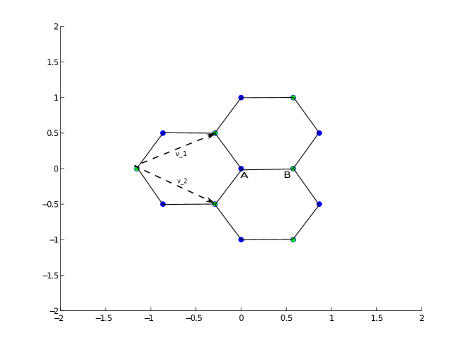
Fig. 1: Part of the honeycomb structure, ${\bf H}$. ${\bf H}$ is the union of two sub-lattices $\Lambda_{\bf A}={\bf A}+\Lambda_{h}$ (blue) and $\Lambda_{\bf B}={\bf B}+\Lambda_{h}$ (green). The lattice vectors $\{{\bf v}_{1},{\bf v}_{2}\}$ generate $\Lambda_{h}$.

.

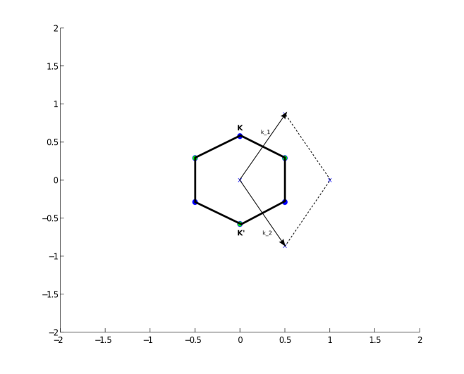
Fig. 2: Brillouin zone, ${\mathcal{B}}$, and dual basis $\{{\bf k}_{1},{\bf k}_{2}\}$. ${\bf K}$ and ${\bf K}^{\prime}$ are labeled. Other vertices of ${\mathcal{B}}_{h}$ obtained via application of $R$, rotation by $2\pi/3$; see equation (53).

.

The dual lattice $\Lambda_{h}^{*}=\ \mathbb{Z}{\bf k}_{1}\oplus\mathbb{Z}{\bf k}_{2}$ is spanned by the dual basis vectors:

$${\bf k}_{1}=\ q\left(\begin{array}[]{c}\frac{1}{2}\\ {}\hfil\\ \frac{\sqrt{3}}{2}\end{array}\right),\ \ \ {\bf k}_{2}=q\ \left(\begin{array}[]{c}\frac{1}{2}\\ {}\hfil\\ -\frac{\sqrt{3}}{2}\end{array}\right),\ \ \ q\equiv\frac{4\pi}{a\sqrt{3}}\ ,$$ (47)

where

$${\bf k}_{\ell}\cdot{\bf v}_{{\ell^{\prime}}}=2\pi\delta_{\ell\ell^{\prime}}\ ,$$ (48)

$$|{\bf v}_{1}|=|{\bf v}_{2}|=a,\ \ {\bf v}_{1}\cdot{\bf v}_{2}=\frac{a^{2}}{2}\ ,$$ (49)

$$|{\bf k}_{1}|=|{\bf k}_{2}|=q,\ \ {\bf k}_{1}\cdot{\bf k}_{2}=-\frac{1}{2}q^{2}\ .$$ (50)

The Brillouin zone, ${\mathcal{B}}$, is a hexagon in $\mathbb{R}^{2}$; see Figure 2. Denote by ${\bf K}$ and ${\bf K^{\prime}}$ the vertices of ${\mathcal{B}}$ given by:

$${\bf K}\equiv\frac{1}{3}\left({\bf k}_{1}-{\bf k}_{2}\right),\ \ {\bf K^{\prime}}\equiv-{\bf K}=\frac{1}{3}\left({\bf k}_{2}-{\bf k}_{1}\right)\ .$$ (51)

All six vertices of ${\mathcal{B}}$ can be generated by application of the rotation matrix, $R$, which rotates a vector in $\mathbb{R}^{2}$ clockwise by $2\pi/3$. $R$ is given by

$$R\ =\ \left(\begin{array}[]{cc}-\frac{1}{2}&\frac{\sqrt{3}}{2}\\ {}\hfil&{}\hfil\\ -\frac{\sqrt{3}}{2}&-\frac{1}{2}\end{array}\right)$$ (52)

and the vertices of ${\mathcal{B}}$ fall into two groups, generated by action of $R$ on ${\bf K}$ and ${\bf K}^{\prime}$:

$${\bf K}\ {\rm type-points:}\ {\bf K},\ R{\bf K}={\bf K}+{\bf k}_{2},\ R^{2}{\bf K}={\bf K}-{\bf k}_{1}$$

$${\bf K^{\prime}}\ {\rm type-points:}\ {\bf K^{\prime}},\ R{\bf K^{\prime}}={\bf K}^{\prime}-{\bf k}_{2},\ R^{2}{\bf K^{\prime}}={\bf K^{\prime}}+{\bf k}_{1}\ .$$ (53)

Remark 2.3 (Symmetry Reduction).

Let $(\ \Phi({\bf x};{\bf k}),\mu({\bf k})\ )$ denote a Floquet-Bloch eigenpair for the eigenvalue problem (17)-(18) with quasi-momentum ${\bf k}$. Since $V$ is real, $(\ \tilde{\Phi}({\bf x};{\bf k})\equiv\overline{\Phi({\bf x};{\bf k})},\mu({\bf k})\ )$ is a Floquet-Bloch eigenpair for the eigenvalue problem with quasi-momentum $-{\bf k}$. Recall the relations (53) and the $\Lambda_{h}^{*}$- periodicity of: ${\bf k}\mapsto\mu({\bf k})$ and ${\bf k}\mapsto\Phi({\bf x};{\bf k})$. It follows that the local character of the dispersion surfaces in a neighborhood of any vertex of ${\mathcal{B}}$ is determined by its character about any other vertex of ${\mathcal{B}}$.

We reminder the reader that below, it will be convenient to work with ${\mathcal{B}}_{h}={\bf K}+{\mathcal{B}}$ as our Brillouin zone, explained in Remark 2.2.

2.3 Honeycomb lattice potentials

For any function $f$, defined on $\mathbb{R}^{2}$, introduce

$$\mathcal{R}[f]({\bf x})=f(R^{*}{\bf x}),$$ (54)

where $R$ is the $2\times 2$ rotation matrix displayed in (52).

Definition 2 (Honeycomb lattice potentials).

Let $V$ be real-valued and $V\in C^{\infty}(\mathbb{R}^{2})$. $V$ is a honeycomb lattice potential if there exists ${\bf x}_{0}\in\mathbb{R}^{2}$ such that $\tilde{V}({\bf x})=V({\bf x}-{\bf x}_{0})$ has the following properties:

1. $\tilde{V}$ is $\Lambda_{h}-$ periodic, i.e. $\tilde{V}({\bf x}+{\bf v})=\tilde{V}({\bf x})$ for all ${\bf x}\in\mathbb{R}^{2}$ and ${\bf v}\in\Lambda_{h}$.

2. $\tilde{V}$ is even or inversion-symmetric, i.e. $\tilde{V}(-{\bf x})=\tilde{V}({\bf x})$.

3. $\tilde{V}$ is $\mathcal{R}$- invariant, i.e.

   $$\mathcal{R}[\tilde{V}]({\bf x})\ \equiv\ \tilde{V}(R^{*}{\bf x})\ =\ \tilde{V}({\bf x}),$$

   where, $R^{*}$ is the counter-clockwise rotation matrix by $2\pi/3$, i.e. $R^{*}=R^{-1}$, where $R$ is given by (52).

Thus, a honeycomb lattice potential is smooth, $\Lambda_{h}$- periodic and, with respect to some origin of coordinates, both inversion symmetric and $\mathcal{R}$- invariant.

Remark 2.4.

As the spectral properties are independent of translation of the potential we shall assume in the proofs, without any loss of generality, that ${\bf x}_{0}=0$.

Remark 2.5.

A consequence of a honeycomb lattice potential being real-valued and even is that if $\left(\Phi({\bf x};{\bf k}),\mu\right)$ is an eigenpair with quasimomentum ${\bf k}$ of the Floquet-Bloch eigenvalue problem, then $\left(\overline{\Phi(-{\bf x};{\bf k})},\mu\right)$ is also an eigenpair with quasimomentum ${\bf k}$.

A key property of honeycomb lattice potentials, $V_{h}$, used in our spectral analysis of $-\Delta+V_{h}$ [10], is that if ${\bf K}_{\star}$ denotes any vertex of ${\mathcal{B}}_{h}$, then we have the commutation relation:

$$\left[\mathcal{R},H_{V_{h}}({\bf K}_{\star})\right]\ =\ 0\ .$$ (55)

It is therefore natural to the split $L^{2}_{{\bf K}_{\star}}$, the space of ${\bf K}_{\star}$- pseudo-periodic functions, into the direct sum:

$$L^{2}_{{\bf K}_{\star}}\ =\ L^{2}_{{\bf K}_{\star},1}\oplus L^{2}_{{\bf K}_{\star},\tau}\oplus L^{2}_{{\bf K}_{\star},\overline{\tau}},$$ (56)

where $L^{2}_{{\bf K}_{\star},\sigma}$ are invariant eigen-subspaces of $\mathcal{R}$, i.e. for $\sigma=1,\tau,\overline{\tau}$, where $\tau=\exp(2\pi i/3)$, and

$$L^{2}_{{\bf K}_{\star},\sigma}\ =\ \Big{\{}g\in L^{2}_{{\bf K}_{\star}}:\mathcal{R}g=\sigma g\Big{\}}\ .$$ (57)

3 Dirac points

We begin with a precise definition of a Dirac point.

Definition 3.

Let $V({\bf x})$ be a smooth, real-valued, even (inversion symmetric) and periodic potential on $\mathbb{R}^{2}$. Denote by ${\mathcal{B}}$ the Brillouin zone given in Remark 2.2. We call ${\bf K}\in{\mathcal{B}}$ a Dirac point if the following holds: There exist an integer $b_{1}\geq 1$, a real number $\mu_{\star}$, and strictly positive numbers, $\lambda$ and $\delta$, such that:

1. $\mu_{\star}$ is a degenerate eigenvalue of $H$ with ${\bf K}-$ pseudo-periodic boundary conditions.

2. $\textrm{dim Nullspace}\Big{(}H-\mu_{\star}I\Big{)}\ =\ 2$

3. $\textrm{Nullspace}\Big{(}H-\mu_{\star}I\Big{)}\ =\ {\rm span}\Big{\{}\Phi_{1}({\bf x}),\Phi_{2}({\bf x})\Big{\}}$, where $\Phi_{1}\in L^{2}_{{\bf K},\tau}$ and $\Phi_{2}({\bf x})=\overline{\Phi_{1}(-{\bf x})}\in L^{2}_{{\bf K},\bar{\tau}}$.

4. There exist Lipschitz functions $\mu_{\pm}({\bf k})$,

   $$\mu_{b_{1}}({\bf k})=\mu_{-}({\bf k})\ \ \ \mu_{b_{1}+1}({\bf k})=\mu_{+}({\bf k}),\ \ \mu_{\pm}({\bf K})=\mu_{\star}$$

   and $E_{\pm}({\bf k})$, defined for $|{\bf k}-{\bf K}|<\delta$, and ${\bf k}-$ pseudo-periodic eigenfunctions of $H$: $\Phi_{\pm}({\bf x};{\bf k})$, with corresponding eigenvalues $\mu_{\pm}({\bf k})$ such that

   $$\mu_{+}({\bf k})-\mu_{\star}\ =\ +\ \lambda\ \left|{\bf k}-{\bf K}\right|\ \left(\ 1\ +\ E_{+}({\bf k})\ \right)\ \ {\rm and}$$

   $$\mu_{-}({\bf k})-\mu_{\star}\ =\ -\ \lambda\ \left|{\bf k}-{\bf K}\right|\ \left(\ 1\ +\ E_{-}({\bf k})\ \right),$$ (58)

   where $|E_{\pm}({\bf k})|\leq C|{\bf k}-{\bf K}|$ for some $C>0$.

Remark 3.1.

In [10] we prove the following

Proposition 4.

Suppose conditions $1.,2.$ and $3.$ of Definition 3 hold and denote by $\{c({\bf m})\}_{{\bf m}\in\mathcal{S}}$ the sequence of $L^{2}_{{\bf K},\tau}$ Fourier-coefficients of $\Phi_{1}({\bf x})$. Define the sum

$$\lambda_{\sharp}\ \equiv\ \sum_{{\bf m}\in\mathcal{S}}c({\bf m})^{2}\ \left(\begin{array}[]{c}1\\ i\end{array}\right)\cdot{\bf K}_{\star}^{\bf m}\ \ ,$$ (59)

with $\mathcal{S}\subset\mathbb{Z}^{2}$; see [10]. If $\lambda_{\sharp}\neq 0$, then $4.$ of Definition 3 holds (see (58) ) with $\lambda=|\lambda_{\sharp}|$.

We next recall the statement of Theorem 5.1 of [10] concerning the existence of Dirac points for the Schrödinger operator with a generic honeycomb lattice potentials.

Theorem 3.1.

Let $V_{h}({\bf x})$ honeycomb lattice potential. Assume further that the Fourier coefficient of $V_{h}$, $V_{1,1}$, is non-vanishing, i.e.

$$V_{1,1}\ \equiv\ \int_{\Omega}e^{-i(k_{1}+k_{2})\cdot{\bf y}}\ V_{h}({\bf y})\ d{\bf y}\ \neq 0\ .$$ (60)

Consider the one-parameter family of honeycomb Schrödinger operators defined by:

$$H^{(\epsilon)}\ \equiv\ -\Delta+\epsilon\ V_{h}({\bf x})\ .$$ (61)

There exists a countable and closed set $\tilde{\mathcal{C}}\subset\mathbb{R}$ such that for all $\epsilon\notin\tilde{\mathcal{C}}$, the vertices, ${\bf K}_{\star}$, of ${\mathcal{B}}_{h}$ are Dirac points in the sense of Definition 3.

More specifically, the following holds for $\epsilon\notin\tilde{\mathcal{C}}$: There exists $b_{1}\geq 1$ such that $\mu_{\star}\equiv\mu^{\epsilon}_{b_{1}}({\bf K}_{\star})=\mu^{\epsilon}_{b_{1}+1}({\bf K}_{\star})$ is a ${\bf K}_{\star}-$ pseudo-periodic eigenvalue of multiplicity two where

1. $\mu^{\epsilon}_{\star}$ is an $L^{2}_{{\bf K},\tau}$ - eigenvalue of $H^{(\epsilon)}$ of multiplicity one, and corresponding eigenfunction, $\Phi^{\epsilon}_{1}({\bf x})$.

   $\mu^{\epsilon}_{\star}$ is an $L^{2}_{{\bf K},\bar{\tau}}$ - eigenvalue of $H^{(\epsilon)}$ of multiplicity one, with corresponding eigenfunction, $\Phi^{\epsilon}_{2}({\bf x})=\overline{\Phi^{\epsilon}_{1}(-{\bf x})}$.

   $\mu^{\epsilon}_{\star}$ is not an $L^{2}_{{\bf K},1}$- eigenvalue of $H^{(\epsilon)}$.

2. There exist $\delta_{\epsilon}>0,\ C_{\epsilon}>0$ and Floquet-Bloch eigenpairs: $(\Phi_{+}^{\epsilon}({\bf x};{\bf k}),\mu_{+}^{\epsilon}({\bf k}))$ and $(\Phi_{-}^{\epsilon}({\bf x};{\bf k}),\mu_{-}^{\epsilon}({\bf k}))$, and Lipschitz continuous functions, $E_{\pm}({\bf k})$, defined for $|{\bf k}-{\bf K}_{\star}|<\delta_{\epsilon}$, such that

   $$\mu^{\epsilon}_{+}({\bf k})-\mu^{\epsilon}({\bf K}_{\star})\ =\ +\ |\lambda^{\epsilon}_{\sharp}|\ \left|{\bf k}-{\bf K}_{\star}\right|\ \left(\ 1\ +\ E^{\epsilon}_{+}({\bf k})\ \right)\ \ {\rm and}$$

   $$\mu^{\epsilon}_{+}({\bf k})-\mu^{\epsilon}({\bf K}_{\star})\ =\ -\ |\lambda^{\epsilon}_{\sharp}|\ \left|{\bf k}-{\bf K}_{\star}\right|\ \left(\ 1\ +\ E^{\epsilon}_{-}({\bf k})\ \right),$$

   where

   $$\lambda_{\sharp}^{\epsilon}\ \equiv\ \sum_{{\bf m}\in\mathcal{S}}c({\bf m},\mu^{\epsilon},\epsilon)^{2}\ \left(\begin{array}[]{c}1\\ i\end{array}\right)\cdot{\bf K}_{\star}^{\bf m}\ \neq\ 0$$ (62)

   is given in terms of $\{c({\bf m},\mu^{\epsilon},\epsilon)\}$, the $L^{2}_{{\bf K},\tau}$- Fourier coefficients of $\Phi^{\epsilon}({\bf x};{\bf K}_{\star})$.

   Furthermore, $|E_{\pm}^{\epsilon}({\bf k})|\leq C_{\epsilon}|{\bf k}-{\bf K}_{\star}|$. Thus, in a neighborhood of the point $({\bf k},\mu)=({\bf K}_{\star},\mu_{\star}^{\epsilon})\in\mathbb{R}^{3}$, the dispersion surface is closely approximated by a circular cone.

3. There exists $\epsilon^{0}>0$, such that for all $\epsilon\in(-\epsilon^{0},\epsilon^{0})\setminus\{0\}$
   (i)  $\epsilon V_{1,1}>0\ \implies$ conical intersection of $1^{st}$ and $2^{nd}$ dispersion surfaces
   (ii) $\epsilon V_{1,1}<0\ \implies$ conical intersection of $2^{nd}$ and $3^{rd}$ dispersion surfaces .

Our point of departure in this paper will be a periodic Schrödinger operator, $-\Delta+V({\bf x})$, where $V$ is a honeycomb lattice potential. We fix a Dirac point, ensured to exist by Theorem 3.1, and study the large time dynamics of wave-packets which are initially (for $t=0$) spectrally localized near these points. Thus we have two band dispersion surfaces, ${\bf k}\in{\mathcal{B}}\mapsto\mu_{b_{1}}({\bf k})\equiv\mu_{-}({\bf k})$ and ${\bf k}\mapsto\mu_{b_{1}+1}({\bf k})\equiv\mu_{+}({\bf k})$ which touch conically at ${\bf k}={\bf K}_{\star}$ with $\mu_{\pm}({\bf K}_{\star})=\mu_{\star}$.

Let

$$\Phi_{1}({\bf x})\ =_{\rm def}\ \Phi_{+}({\bf x})\ \in L^{2}_{{\bf K}_{\star},\tau}$$

$$\Phi_{2}({\bf x})\ =\ \overline{\Phi_{1}(-{\bf x})}\ =_{\rm def}\ \Phi_{-}({\bf x})\in L^{2}_{{\bf K}_{\star},\bar{\tau}}$$ (63)

span the two-dimensional subspace of the degenerate eigenvalue $\mu_{\star}$ for $H$:

$$H\Phi_{j}({\bf x})\ \equiv\ \left(-\Delta+V\right)\Phi_{j}=\ \mu_{\star}\Phi_{j}$$ (64)

$$\Phi_{j}({\bf x}+{\bf v})\ =\ e^{i{\bf K}_{\star}\cdot{\bf v}}\ \Phi_{j}({\bf x}),\ \ {\bf x}\in\mathbb{R}^{2},\ \ \ {\bf v}\in\Lambda_{h}$$ (65)

We also define the periodic vectors:

$$p_{1}({\bf x})=e^{-i{\bf K}_{\star}\cdot{\bf x}}\Phi_{1}({\bf x}),\ \ p_{2}({\bf x})=e^{-i{\bf K}_{\star}\cdot{\bf x}}\Phi_{2}({\bf x})\ .$$ (66)

We choose these states to be orthonormal

$$\left\langle\Phi_{l},\Phi_{m}\right\rangle_{L^{2}(\Omega)}\ =\ \delta_{lm}\ ,\ \ \ l,m=1,2\ .$$

To study the time evolution (2) we expand the solution of the initial value problem with data $\psi_{0}$ using the complete set of Floquet-Bloch modes:

$$e^{-iHt}\ \psi_{0}\ =\ \sum_{b\geq 1}\ \int_{\mathcal{B}_{h}}\ e^{-i\mu_{b}({\bf k})t}\ \langle\Phi_{b}(\cdot;{\bf k}),\psi_{0}(\cdot)\rangle\ \Phi_{b}({\bf x};{\bf k})\ d{\bf k}$$ (67)

Suppose $H$ has a Dirac point, ${\bf K}$. We remark that in (67) we choose the Brillouin zone, ${\mathcal{B}}_{h}={\mathcal{B}}+{\bf K}$, which is centered at ${\bf K}$; see Remark 2.2. For initial conditions which are spectrally supported near ${\bf K}$, the time evolution depends on the precise behavior of the Floquet-Bloch modes $\Phi_{\pm}({\bf x};{\bf k})$ for ${\bf k}$ near ${\bf K}$. While Theorem 3.1 shows that the eigenvalues $\mu_{\pm}({\bf k})$ are Lipschitz functions in a small neighborhood of ${\bf k}={\bf K}$, the eigenfunctions $\Phi_{\pm}({\bf x};{\bf k})$ are not continuous functions of ${\bf k}$ in a neighborhood of ${\bf K}$.

Theorem 3.2.

Let ${\bf K}$ denote a Dirac point in the sense of Definition 3. In particular, let $(\Phi_{\pm}({\bf x};{\bf k}),\mu_{\pm}({\bf k}))$ denote the ${\bf k}-$ pseudo-periodic eigenpairs as in part 4 of Definition 3. Introduce the $\Lambda_{h}-$ periodic functions $p_{\pm}({\bf x};{\bf k})$ by

$$\Phi_{\pm}({\bf x};{\bf k})\ =\ e^{i{\bf k}\cdot{\bf x}}\ p_{\pm}({\bf x};{\bf k}),\ \ \left\langle p_{a}(\cdot;{\bf k}),p_{b}(\cdot;{\bf k})\right\rangle=\delta_{ab},\ a,b\in\{+,-\}\ .$$ (68)

Let ${\bf k}={\bf K}+{\mathbf{\kappa}}$. Then, for $0<|{\mathbf{\kappa}}|<\delta$ and $p_{j}$ given by (66) we have:

$$\mu_{\pm}({\bf K}+\kappa)\ =\ \mu_{\star}\ \pm\ |\lambda_{\sharp}|\ (\kappa_{1}^{2}+\kappa_{2}^{2})^{1\over 2}\ +\ \mathcal{O}\Big{(}\kappa_{1}^{2}+\kappa_{2}^{2}\Big{)},\$$ (69)

and $p_{\pm}({\bf x};{\bf k})$, a priori defined up to an arbitrary (complex) multiplicative constant of absolute value $1$, can be chosen so that:

$$p_{\pm}({\bf x};{\bf K}+{\mathbf{\kappa}})\ =\ \frac{1}{\sqrt{2}}\ \frac{\kappa_{1}+i\kappa_{2}}{(\kappa_{1}^{2}+\kappa_{2}^{2})^{1\over 2}}\ p_{1}({\bf x})\ \pm\ \frac{1}{\sqrt{2}}\ p_{2}({\bf x})$$

$$\qquad\qquad+\ \mathcal{O}_{H^{2}(\mathbb{R}^{2}/\Lambda_{h})}\Big{(}(\kappa_{1}^{2}+\kappa_{2}^{2})^{1\over 2}\Big{)}\ .$$ (70)

Proof of Theorem 3.2: The proof builds on the proof of Theorem 4.1 of [10], in which the ${\bf k}-$ pseudo-periodic eigenvalues, $\mu_{\pm}({\bf k})$, are constructed. These were shown to be Lipschitz continuous functions for ${\bf k}$ varying in a neighborhood of ${\bf K}$. We now consider the associated Floquet-Bloch modes.

Let ${\bf k}-$ pseudo-periodic Floquet-Bloch modes can be expressed in the form

$$\Phi({\bf x};{\bf k})=e^{i{\bf k}\cdot{\bf x}}p({\bf x};{\bf k}),$$

where $p({\bf x};{\bf k})$ is $\Lambda_{h}$ periodic. Since we are interested in the character of $p({\bf x};{\bf k})$ for ${\bf k}$ near ${\bf K}$ we set: ${\bf k}={\bf K}+{\mathbf{\kappa}}$. Then, $p({\bf x};{\bf K}+\kappa)$ satisfies the periodic eigenvalue problem:

$$H({\bf K}+{\mathbf{\kappa}})\ p({\bf x};{\bf K}+{\mathbf{\kappa}})\ =\ \mu({\bf K}+{\mathbf{\kappa}})\ p({\bf x};{\bf K}+{\mathbf{\kappa}})\ ,$$ (71)

$$p({\bf x}+{\bf v};{\bf K}+{\mathbf{\kappa}})=p({\bf x};{\bf K}+{\mathbf{\kappa}}),\ \ \textrm{for all}\ {\bf v}\in\Lambda_{h}\ ,$$ (72)

where

$$H({\bf k})\ \equiv\ -\left(\nabla_{\bf x}+i{\bf k}\right)^{2}\ +\ V({\bf x})\ .$$

The eigenvalue problem (71)-(72) has eigenvalues, computed via degenerate perturbation theory of the double eigenvalue $\mu_{\star}$ of $H({\bf K})$, given by:

$$\mu_{\pm}({\bf K}+{\mathbf{\kappa}}) =\ \mu_{\star}\ +\ \mu^{(1)}\$$ (73)

$$\mu^{(1)}\ =\ \pm|\lambda_{\sharp}|\ |\kappa|\ +\ \mathcal{O}(|{\mathbf{\kappa}}|^{2})\ .$$ (74)

Denote by $Q_{\perp}$ the projection onto the orthogonal complement of ${\rm span}\{p_{1},p_{2}\}$. Then,

$$R_{\bf K}(\mu_{\star})\ \equiv\ \left(\ H({\bf K})\ -\mu_{\star}\ I\right)^{-1}:\ Q_{\perp}L^{2}(\mathbb{R}^{2}/\Lambda_{h})\to Q_{\perp}L^{2}(\mathbb{R}^{2}/\Lambda_{h})$$

is bounded. Furthermore, via Lyapunov-Schmidt reduction of the eigenvalue problem (71)-(72) we obtain, corresponding to the eigenvalues $\mu_{\pm}({\bf K}+{\mathbf{\kappa}})$ the Floquet-Bloch modes:

$$p_{\pm}({\bf x};{\bf K}+{\mathbf{\kappa}})\ =\ \Big{(}\ I\ +\ R_{\bf K}(\mu_{\star})\ Q_{\perp}\ \left(2i{\mathbf{\kappa}}\cdot\left(\nabla+i{\bf K}\right)\right)\ \Big{)}\left(\ \alpha p_{1}({\bf x})\ +\ \beta p_{2}({\bf x})\ \right)$$

$$\qquad\qquad+\mathcal{O}_{H^{2}(\mathbb{R}^{2}/\Lambda_{h})}\left(|\kappa|(|\alpha|^{2}+|\beta|^{2})^{1\over 2}\right)\ .$$ (75)

The ${\mathbf{\kappa}}-$ dependent coefficients $\alpha$ and $\beta$ satisfy the homogeneous equation

$$\mathcal{M}(\mu^{(1)},\kappa)\ \left(\begin{array}[]{c}\alpha\\ {}\hfil\\ \beta\end{array}\right)\ =\ 0\ ,$$ (76)

where $\mathcal{M}(\mu^{(1)},\kappa)$ is a $2\times 2$ matrix of the form:

$$\mathcal{M}(\mu^{(1)},\kappa) \equiv\ \left(\begin{array}[]{cc}\mu^{(1)}+\mathcal{O}\left(|\kappa|^{2}\right)&-\overline{\lambda_{\sharp}}(\kappa_{1}+i\kappa_{2})+\mathcal{O}\left(|\kappa|^{2}\right)\\ &\\ -\lambda_{\sharp}(\kappa_{1}-i\kappa_{2})+\mathcal{O}\left(|\kappa|^{2}\right)&\mu^{(1)}+\mathcal{O}\left(|\kappa|^{2}\right)\end{array}\right)\ \ ;$$ (79)

see [10] for the derivation of (75)-(76).

The Floquet-Bloch modes, $p_{\pm}({\bf x};{\bf k})$, are finally determined by the solutions $\alpha=\alpha_{\pm}({\mathbf{\kappa}})$, $\beta=\beta_{\pm}({\mathbf{\kappa}}))$ of the homogeneous algebraic system (76) for the choices $\mu^{(1)}_{\pm}({\mathbf{\kappa}})$ in (74). We select (normalized) solutions of (76) as follows:

$$\mu^{(1)}_{\pm} =\pm|\lambda_{\sharp}|\ |{\mathbf{\kappa}}|+\mathcal{O}(|{\mathbf{\kappa}}|^{2}),$$

$$\left(\begin{array}[]{c}\alpha_{\pm}\\ \beta_{\pm}\end{array}\right)\ =\ \left(\begin{array}[]{c}\frac{1}{\sqrt{2}}\ \frac{\overline{\lambda_{\sharp}}}{|\lambda_{\sharp}|}\ \frac{\kappa_{1}+i\kappa_{2}}{(\kappa_{1}^{2}+\kappa_{2}^{2})^{1\over 2}}+\mathcal{O}\left((\kappa_{1}^{2}+\kappa_{2}^{2})^{1\over 2}\right)\\ \pm\frac{1}{\sqrt{2}}\ +\ \mathcal{O}\left((\kappa_{1}^{2}+\kappa_{2}^{2})^{1\over 2}\right)\end{array}\right)\ .$$ (84)

Here, we take advantage of the observation that for a rank-1 matrix

$$\mathcal{A}\ =\ \left(\begin{array}[]{cc}A&B\\ C&D\end{array}\right)\ \textrm{the vector}\left(\begin{array}[]{c}B\\ -A\end{array}\right)$$

lies in the nullspace of $\mathcal{A}$.

Thus, with ${\mathbf{\kappa}}\equiv{\bf k}-{\bf K}$, we have upon substitution of (84) into (75) the expansions of $\mu_{\pm}({\bf k})$ and $p_{\pm}({\bf x};{\bf k})$ in (69) and (70).

4 2D Dirac equation

In this section we collect results on well-posedness and estimates on solutions of the two-dimensional Dirac system (5)-(6). Taking the Fourier transform of (5)-(6) we obtain for $\alpha(\Xi,T)=\alpha(\xi_{1},\xi_{2},T)$ the equation

$$i\partial_{T}\left(\begin{array}[]{c}\hat{\alpha}_{1}\\ \hat{\alpha}_{2}\end{array}\right)\ =\ \Omega(\Xi)\ \left(\begin{array}[]{c}\hat{\alpha}_{1}\\ \hat{\alpha}_{2}\end{array}\right),\ \ \textrm{where}$$ (89)

$$\Omega(\Xi)\ =\ \left(\begin{array}[]{cc}0&\overline{\lambda_{\sharp}}(\xi_{1}+i\xi_{2})\\ \lambda_{\sharp}(\xi_{1}-i\xi_{2})&0\end{array}\right)\ =\ \Omega(\Xi)^{*}\ .$$ (92)

Remark 4.1.

It follows from (92) that the dispersion relation for (5)-(6) is:

$$\omega^{2}(\xi_{1},\xi_{2})=|\lambda_{\sharp}|^{2}\ \left(\xi_{1}^{2}+\xi_{2}^{2}\right)\ ;$$

the effective dynamics are non-dispersive.

Remark 4.2.

The system (5)-(6) has the structure of Dirac system:

$$i\partial_{t}\left(\begin{array}[]{c}\alpha_{1}\\ \alpha_{2}\end{array}\right)\ =\ \left[\ \sigma_{1}^{\sharp}\ \frac{1}{i}\frac{\partial}{\partial X_{1}}\ -\ \sigma_{2}^{\sharp}\ \frac{1}{i}\frac{\partial}{\partial X_{2}}\ \right]\ \left(\begin{array}[]{c}\alpha_{1}\\ \alpha_{2}\end{array}\right)\ .$$ (93)

The $2\times 2$ matrices $\sigma_{1}^{\sharp}$ and $\sigma_{2}^{\sharp}$ satisfy the relations

$$(\sigma_{j}^{\sharp})^{2}\ =\ |\lambda_{\sharp}|^{2}\ Id,\ \ {\rm and}\ \ \sigma_{1}^{\sharp}\sigma_{2}^{\sharp}\ +\ \sigma_{2}^{\sharp}\sigma_{1}^{\sharp}\ =\ 0\ .$$

Here, $\sigma_{j}^{\sharp},\ j=1,2$ are given by the Hermitean matrices:

$$\sigma_{1}^{\sharp}\ \equiv\ \Lambda_{\sharp}\sigma_{1},\ \ \sigma_{2}^{\sharp}\ \equiv\ \Lambda_{\sharp}\sigma_{2}\ ,$$ (94)

in terms of $\Lambda_{\sharp}$ and the standard Pauli matrices $\sigma_{1}$ and $\sigma_{2}$ :

$$\Lambda_{\sharp}\ =\ \left(\begin{array}[]{cc}\overline{\lambda_{\sharp}}&0\\ 0&\lambda_{\sharp}\end{array}\right),\ \ \sigma_{1}\ =\ \left(\begin{array}[]{cc}0&1\\ 1&0\end{array}\right),\ \ \sigma_{2}\ =\ \left(\begin{array}[]{cc}0&-i\\ i&0\end{array}\right)$$ (101)

Finally, note that $\alpha_{j},\ j=1,2$ satisfy the two-dimensional wave equation, with wave-speed $|\lambda_{\sharp}|$:

$$\partial^{2}_{t}\alpha\ =|\lambda_{\sharp}|^{2}\left(\frac{\partial^{2}}{\partial X_{1}^{2}}+\frac{\partial^{2}}{\partial X_{2}^{2}}\right)\alpha\ .$$

Proposition 5.

Assume $\alpha({\bf X},0)=\alpha_{0}({\bf X})\in\left(H^{s}(\mathbb{R}^{2})\right)^{2}$. Then,

$$\partial_{T}^{k}\alpha\in L^{\infty}\left([0,\infty)\ ;\ \left(H^{s-k}(\mathbb{R}^{2})\right)^{2}\right),\ \textrm{for}\ 0\leq k\leq s\ .$$

In particular,

1. The Fourier transform of the solution, $\alpha({\bf X},T)$ is given explicitly by

   $$\hat{\alpha}(\Xi,T)\ =\ e^{-i\Omega(\Xi)T}\ \hat{\alpha}_{0}(\Xi),\ \ \Omega(\Xi)^{*}=\Omega(\Xi)$$

2. For all $\Xi\in\mathbb{R}^{2}$,  $\left|\hat{\alpha}(\Xi,T)\right|\ =\ \left|\hat{\alpha}_{0}(\Xi)\right|$ and therefore

3. For any ${\bf a}\in\mathbb{Z}^{2}$ with $|{\bf a}|\leq s$

   $$\left\|\ \partial^{\bf a}_{\bf X}\alpha({\bf X},T)\ \right\|_{L^{2}(\mathbb{R}^{2})}\ =\ \ \left\|\ \partial^{\bf a}_{\bf X}\alpha({\bf X},0)\ \right\|_{L^{2}(\mathbb{R}^{2})}$$ (102)

5 Effective Dirac dynamics; statement of main result, Theorem 6

A general solution of the time-dependent Schrödinger equation, constrained to the degenerate $2$-dimensional eigenspace associated with eigenvalue, $\mu_{\star}=\mu({\bf K}_{\star})$, associated with the Dirac point, ${\bf K}_{\star}$, is of the form

$$\psi({\bf x},t)=e^{-i\mu_{\star}t}\ \left(\ \alpha_{1}\ \Phi_{1}({\bf x})+\alpha_{2}\ \Phi_{2}({\bf x})\ \right),$$ (103)

where $\alpha_{1}$ and $\alpha_{2}$ are arbitrary constants.

Consider now a wave packet initial condition, which is spectrally concentrated near ${\bf K}_{\star}$:

$$\psi^{\delta}({\bf x},0)\ =\ \psi_{0}^{\delta}({\bf x})\ =\ \delta\ \left(\ \alpha_{10}(\delta{\bf x})\ \Phi_{1}({\bf x})+\alpha_{20}(\delta{\bf x})\ \Phi_{2}({\bf x})\ \right)$$

$$=\delta\ \left(\ \alpha_{10}(\delta{\bf x})\ p_{1}({\bf x})+\alpha_{20}(\delta{\bf x})\ p_{2}({\bf x})\ \right)\ e^{i{\bf K}_{\star}\cdot{\bf x}}\$$ (104)

Here, $\delta$ is a small parameter. We assume $\alpha_{10}({\bf X})$ and $\alpha_{20}({\bf X})$ are Schwartz functions of ${\bf X}$. We expect that this assumption can be weakend considerably without difficulty. The overall factor of $\delta$ in (104) is not essential (the problem is linear), but is inserted so that $\psi^{\delta}_{0}$ has $L^{2}(\mathbb{R}^{2})$- norm of order of magnitude one.

We seek solutions of (2), (104) in the form:

$$\psi^{\delta}({\bf x},t)=e^{-i\mu_{\star}t}\left(\sum_{j=1}^{2}\ \delta\ \alpha_{j}(\delta{\bf x},\delta t)\Phi_{j}({\bf x})+\eta^{\delta}({\bf x},t)\right).$$ (105)

$$\textrm{where}\ \eta^{\delta}({\bf x},0)=0,\ \alpha_{j}({\bf X},0)=\alpha_{j0}({\bf X}),\ j=1,2$$ (106)

to ensure the initial condition (104).

The goal is to show that the Schrödinger equation (2) has a solution of the form (105) with an error term, $\eta^{\delta}({\bf x},t)$, which satisfies

$$\sup_{0\leq t\leq\rho\delta^{-2+\varepsilon_{1}}}\ \|\ \eta^{\delta}(\cdot,t)\ \|_{H^{s}(\mathbb{R}^{2})}\ =\ \mathcal{O}(\delta^{\tau_{\star}}),\ \ \delta\to 0\ .$$ (107)

for some $\tau_{\star}>0$, provided the slowly varying amplitudes $\alpha_{j}(\delta{\bf x},\delta t),\ j=1,2$ evolve according to the system of Dirac-type equations (5)-(6). Here, $\rho>0$ and $\varepsilon_{1}>0$ are arbitrary.

We shall prove the following

Theorem 6.

Assume

$$\vec{\alpha}_{0}({\bf X})\ \equiv\ \left(\begin{array}[]{c}\alpha_{10}({\bf X})\\ \alpha_{20}({\bf X})\end{array}\right)\in\left[\mathcal{S}(\mathbb{R}^{2})\right]^{2}$$

and let $\vec{\alpha}({\bf X},T)$ denote the global-in-time solution of the Dirac system (5)-(6) with initial data $\vec{\alpha}({\bf X},0)=\vec{\alpha}_{0}({\bf X})$. Consider the time-dependent Schrödinger equation, (2), where $V({\bf x})$ denotes a potential for which the conclusions of Theorem 3.1 hold, e.g. $V({\bf x})=\epsilon V_{h}({\bf x})$, where $V_{h}$ is a honeycomb lattice potential satisfying $V_{1,1}\neq 0$ and $\epsilon$ is not in the countable closed set $\tilde{\mathcal{C}}$. Assume initial conditions, $\psi_{0}$, of the form (104). Fix any $\rho>0$ and $\varepsilon_{1}>0$. Also choose non-negative $N=(n_{1},n_{2})\in\mathbb{Z}^{2}$ with $n_{1},n_{2}\geq 0$. Then, (2) has a unique solution of the form (105), where for any $|\alpha|\leq N$

$$\sup_{0\leq t\leq\rho\ \delta^{-2+\varepsilon_{1}}}\left\|\ \partial_{{\bf x}}^{\alpha}\eta^{\delta}({\bf x},t)\ \right\|_{L^{2}(\mathbb{R}_{\bf x}^{2})}\ \ =\ o(\delta^{\tau_{\star}}),\ \ \delta\to 0\,$$ (108)

for some $\tau_{*}>0$.

6 Proof of Theorem 6

We begin with a summary of consequences of Theorems 3.1 and 3.2 which we use in the proof.

Recall that the spectral bands $\mu_{+}({\mathcal{B}}_{h})$ and $\mu_{-}({\mathcal{B}}_{h})$ touch conically at the the vertices of ${\mathcal{B}}_{h}$. Specifically, $\mu_{+}({\bf k})=\mu_{-}({\bf k})=\mu_{\star}$ for ${\bf k}={\bf K}_{\star}$ equal to any of the three ${\bf K}$- type vertices, $\{{\bf K},R{\bf K},R^{2}{\bf K}\}$ and any of the three ${\bf K}^{\prime}$- type vertices, $\{{\bf K}^{\prime},R{\bf K}^{\prime},R^{2}{\bf K}^{\prime}\}$, where ${\bf K}^{\prime}=-{\bf K}$. Here, $R$ denotes the $\pi/3$- counterclockwise rotation.

For a Dirac point ${\bf K}_{\star}$, equal to any vertex of ${\mathcal{B}}_{h}$:

• There exist $L^{2}_{\bf k}$- eigenvalues of $H$, denoted $\mu_{\pm}({\bf k})$, such that

  $$\textrm{for all}\ {\bf k}\in\mathcal{B}_{h}\ \textrm{ satisfying}\ |{\bf k}-{\bf K}_{\star}|<\kappa_{0}$$

  $$\mu_{\pm}({\bf k})-\mu({\bf K}_{\star})=\pm|\lambda_{\sharp}|\left|{\bf k}-{\bf K}_{\star}\right|\left(1+E_{\pm}({\bf k}-{\bf K}_{\star})\right),$$ (109)

  where $E_{\pm}({\mathbf{\kappa}})$ are Lipschitz continuous in ${\mathbf{\kappa}}$ and $E_{\pm}({\mathbf{\kappa}})\leq C_{\pm}\ |{\mathbf{\kappa}}|$. Here, $\lambda_{\sharp}$ is a constant given by (62).

• There are constants $\kappa_{1},C_{1}$ such that

  $$\textrm{ for all}\ {\bf k}\in\mathcal{B}_{h}\ \textrm{satisfying}\ |{\bf k}-{\bf K}_{\star}|<{\mathbf{\kappa}}_{1}\ \textrm{ and all}\ b\notin\{+,-\}$$

  $$\left|\mu_{b}({\bf k})-\mu({\bf K}_{\star})\right|\geq C_{1}>0.$$ (110)

• For $0<|{\mathbf{\kappa}}|<\delta$ sufficiently small

  $$p_{\pm}({\bf x};{\bf K}_{\star}+{\mathbf{\kappa}})\ =\ \frac{1}{\sqrt{2}}\Big{(}\ \alpha({\mathbf{\kappa}})\ p_{1}({\bf x})\ \pm\ p_{2}({\bf x})\ \Big{)}\ +\ \mathcal{O}_{H^{2}(\mathbb{R}^{2}/\Lambda_{h})}\left(|{\mathbf{\kappa}}|\right),$$ (111)

  $$\ {\rm where}\ \ \alpha({\mathbf{\kappa}})\ =\ \frac{\overline{\lambda_{\sharp}}}{|\lambda_{\sharp}|}\ \frac{{\mathbf{\kappa}}_{1}+i{\mathbf{\kappa}}_{2}}{\sqrt{{\mathbf{\kappa}}_{1}^{2}+{\mathbf{\kappa}}_{2}^{2}}}$$ (112)

(P2) is a consequence of (P1) and the continuity of the eigenvalues ${\bf k}\mapsto\mu_{b}({\bf k})$; see Proposition 1.

Without loss of generality and for simplicity:

1. we take

   $${\bf K}_{\star}={\bf K}$$

2. we recall that the Brillouin zone, ${\mathcal{B}}_{h}$, is centered at ${\bf K}$; see Remark 2.2. Since we assume wave-packet initial data which are spectrally localized near ${\bf K}$ in $\mathbb{R}^{2}/\Lambda^{*}_{h}$, this equivalent choice, which puts ${\bf K}$ on the interior of the Brillouin zone, simplifies the analysis.

To prove Theorem 6, we study the evolution equation for $\eta^{\delta}({\bf x},t)$ obtained by substitution of (105) into (2):

$$i\partial_{t}\eta^{\delta}\ =\ \left(H-\mu_{\star}\right)\eta^{\delta}$$

$$\qquad\ -\delta^{2}\sum_{j=1}^{2}\ \left.\Big{[}\ i\partial_{T}\alpha_{j}({\bf X},T)\ \Phi_{j}({\bf x})+2\nabla_{\bf X}\alpha_{j}({\bf X},T)\cdot\nabla_{\bf x}\Phi_{j}({\bf x})\Big{]}\ \right|_{({\bf X},T)=(\delta{\bf x},\delta t)}$$

$$\qquad\ -\ \delta^{3}\ \sum_{j=1}^{2}\ \Delta_{\bf X}\alpha_{j}({\bf X},T)\Phi_{j}({\bf x})\ \Big{|}_{({\bf X},T)=(\delta{\bf x},\delta t)},$$ (113)

$$\eta^{\delta}({\bf x},t=0)\ =\ 0\ .$$ (114)

6.1 Estimation of the error, $\eta^{\delta}({\bf x},t)$

Using the DuHamel principle we may rewrite (113) as the equivalent integral equation:

$$\eta^{\delta}(\cdot,t)\ =\ i\delta^{2}\ \sum_{j=1}^{2}\ \int_{0}^{t}\ e^{-i(H-\mu_{\star})(t-s)}\ \Big{[}\ i\partial_{S}\alpha_{j}(\delta\cdot,\delta s)\ \Phi_{j}(\cdot)+2\nabla_{\bf X}\alpha_{j}(\delta\cdot,\delta s)\cdot\nabla_{x}\Phi_{j}(\cdot)\ \Big{]}\ ds$$

$$\qquad\ +\ i\delta^{3}\ \sum_{j=1}^{2}\int_{0}^{t}\ e^{-i(H-\mu_{\star})(t-s)}\ \Delta_{\bf X}\alpha_{j}(\delta\cdot,\delta s)\Phi_{j}(\cdot)\ ds$$ (115)

The second integral in (115) (call it $Int_{2}$) can be bounded as follows. Let $s$ denote an even positive integer. Recall from elliptic theory that

$$\|f\|^{2}_{H^{s}}\ \lesssim\ \|f\|_{2}^{2}\ +\ \|(-\Delta+V+c)^{s\over 2}f\|^{2}_{2}\ \lesssim\|f\|^{2}_{H^{s}}\ ,$$ (116)

where $c>\sup_{{\bf x}\in\mathbb{R}^{2}}|V({\bf x})|$. Using (116), we can bound $\|Int_{2}\|_{H^{s}}$ in terms of $\|Int_{2}\|_{L^{2}}$ and $\|(-\Delta+V+c)^{s\over 2}Int_{2}\|_{L^{2}}$. Taking the $L^{2}$ norm of $Int_{2}$ and using that $e^{-iHt}$ is unitary in $L^{2}$, we obtain

$$\|Int_{2}\|_{L^{2}}\lesssim\delta^{3}\sum_{j=1}^{2}\int_{0}^{t}\|\Delta_{\bf X}\alpha_{j}(\delta\cdot,\delta s)\|_{L^{2}}\ ds.$$ (117)

Next, using that $H=-\Delta+V$ commutes with $e^{-iHt}$ we obtain

$$\|(-\Delta+V+c)^{s\over 2}Int_{2}\|_{L^{2}}\lesssim\delta^{3}\sum_{j=1}^{2}\int_{0}^{t}\ \|(-\Delta+V+c)^{s\over 2}\Delta_{\bf X}\alpha_{j}(\delta\cdot,\delta s)\|_{L^{2}}\ ds.$$ (118)

Next note, via Proposition 5, that

$$\|\alpha_{j}(\delta\cdot,\delta t)\|_{H^{m}(\mathbb{R}^{2})}\leq C\delta^{-1}\ \|\alpha_{0}\|_{H^{m}(\mathbb{R}^{2})}\ .$$ (119)

Let $\varepsilon_{1}>0$ be arbitrary. Then, equations (116)-(119) imply

$$\sup_{0\leq t\leq\rho\delta^{-2+\varepsilon_{1}}}\|Int_{2}\|_{H^{s}}$$

$$\equiv\ \sup_{0\leq t\leq\rho\delta^{-2+\varepsilon_{1}}}\ \left\|\ \delta^{3}\ \sum_{j=1}^{2}\int_{0}^{t}\ e^{i(H-\mu_{\star})(t-s)}\ \Delta_{\bf X}\alpha_{j}(\delta\cdot,\delta s)\Phi_{j}(\cdot)\ ds\ \right\|_{H^{s}(\mathbb{R}^{2})}\ \leq\ C\ \rho\ \delta^{\varepsilon_{1}}\ .$$ (120)

It therefore suffices to estimate the first time-integral in (115). This time-integral is the solution of the initial value problem of the form:

$$i\partial_{t}f^{\delta}({\bf x},t)\ -\ \left(H-\mu_{\star}\right)f^{\delta}({\bf x},t)\ =\ \delta^{2}\ \sum_{r}\gamma_{r}(\delta{\bf x},\delta t)\Psi_{r}({\bf x}),$$ (121)

$$f^{\delta}({\bf x},0)=0,$$ (122)

where we find it convenient to introduce the notation

$$\sum_{r}\gamma_{r}({\bf X},T)\Psi_{r}({\bf x})\ \equiv\ -\sum_{j=1}^{2}\ \Big{[}\ i\partial_{T}\alpha_{j}({\bf X},T)\ \Phi_{j}({\bf x})\ +\ 2\nabla_{\bf X}\alpha_{j}({\bf X},T)\cdot\nabla_{\bf x}\Phi_{j}({\bf x})\ \Big{]}\ ,$$ (123)

where

$$\gamma_{1}({\bf X},T)\ =\ i\partial_{T}\alpha_{1}({\bf X},T),\qquad\Psi_{1}({\bf x})=\Phi_{1}({\bf x}),$$ (124)

$$\gamma_{2}({\bf X},T)\ =\ i\partial_{T}\alpha_{2}({\bf X},T),\qquad\Psi_{2}({\bf x})=\Phi_{2}({\bf x}),$$ (125)

$$\gamma_{3}({\bf X},T)\ =\ 2\nabla_{\bf X}\alpha_{1}({\bf X},T),\qquad\Psi_{3}({\bf x})=(\Psi_{3,1}({\bf x}),\Psi_{3,2}({\bf x}))=\nabla_{\bf x}\Phi_{1}({\bf x}),$$ (126)

$$\gamma_{4}({\bf X},T)\ =\ 2\nabla_{\bf X}\alpha_{2}({\bf X},T),\qquad\Psi_{4}({\bf x})=(\Psi_{4,1}({\bf x}),\Psi_{4,2}({\bf x}))=\nabla_{\bf x}\Phi_{2}({\bf x})\ .$$ (127)

Note that $\Psi_{j}({\bf x})\in L^{2}_{\bf K},\ 1\leq j\leq 4$.

By hypotheses on $\alpha_{j}$ and $\Phi_{j}$, and Proposition 5, the functions $\gamma_{r}$ and $\Psi_{r}$ satisfy the following properties:

$$\gamma_{r}({\bf X},T)\ \textrm{is}\ C^{\infty}\left(\mathbb{R}_{T};\mathcal{S}(\mathbb{R}_{\bf X}^{2})\right)\$$ (128)

$$\|\gamma_{r}(\cdot,T)\|_{H^{s}(\mathbb{R}^{2})}\ \lesssim\ \|\alpha(\cdot,T=0)\|_{H^{s+1}}$$ (129)

$$\Psi_{r}({\bf x})\in C^{\infty}(\mathbb{R}_{\bf x}^{2})\cap L^{2}_{{\bf K}}$$

and therefore satisfies the pseudo-periodic boundary condition

$$\Psi_{r}({\bf x}+{\bf v})\ =\ e^{i{\bf K}\cdot{\bf v}}\Psi_{r}({\bf x})\ .$$ (130)

We also write $\Psi_{r}$ in the following useful form:

$$\Psi_{r}({\bf x})\ =\ e^{i{\bf K}\cdot{\bf x}}\mathcal{P}_{r}({\bf x}),\ \ \mathcal{P}_{r}({\bf x}+{\bf v})=\mathcal{P}_{r}({\bf x})\ ,\ {\bf v}\in\Lambda_{h}\ .$$ (131)

By (25), for any $\beta\in\mathbb{N}_{0}^{2}$,

$$\|\partial^{\beta}_{\bf x}\mathcal{P}_{r}\|_{L^{\infty}(\Omega)}\ \leq\ C_{r,\beta}\ .$$ (132)

Theorem 6 is therefore reduced to the following

Proposition 7.

Let $\alpha_{1}({\bf X},T)$ and $\alpha_{2}({\bf X},T)$ satisfy the system of Dirac equations:

$$\partial_{T}\alpha_{1}\ =\ -\overline{\lambda_{\sharp}}\left(\partial_{X_{1}}+i\partial_{X_{2}}\right)\alpha_{2}$$ (133)

$$\partial_{T}\alpha_{2}\ =\ -\lambda_{\sharp}\left(\partial_{X_{1}}-i\partial_{X_{2}}\right)\alpha_{1}$$ (134)

with initial conditions as in Theorem 6. Then, for any $s\geq 1,\rho>0$ and $\varepsilon_{1}>0$, there exists a unique solution, $f^{\delta}({\bf x},t)$ of (121), which satisfies the estimate

$$\sup_{0\leq t\leq\rho\ \delta^{-2+\varepsilon_{1}}}\ \left\|\ f^{\delta}(\cdot,t)\ \right\|_{H^{s}(\mathbb{R}^{2})}\ \leq\ C\ \delta^{\frac{\varepsilon_{1}}{2}},\ {\rm for}\ \delta\downarrow 0\ .$$ (135)

So to finish the proof Theorem 6, we only require a proof of Proposition 7.

7 Proof of Proposition 7

By the completeness of Bloch modes,

$$e^{-i(H-\mu_{\star})t}\ g\ =\ \sum_{b}\ \int_{\mathcal{B}_{h}}\ e^{-i(\mu_{b}({\bf k})-\mu_{\star})t}\ \langle\Phi_{b}(\cdot;{\bf k}),g(\cdot)\rangle_{L^{2}(\mathbb{R}^{2})}\ \Phi_{b}({\bf x};{\bf k})\ d{\bf k}$$ (136)

Thus,

$$f^{\delta}({\bf x},t)=\sum_{b}\ \int_{\mathcal{B}_{h}}\ \tilde{f}^{\delta}_{b}({\bf k},t)\Phi_{b}({\bf x};{\bf k})\ d{\bf k},$$ (137)

where

$$\tilde{f}^{\delta}_{b}({\bf k},t)=-i\delta^{2}\ \int_{0}^{t}\ ds\ e^{-i(\mu_{b}({\bf k})-\mu_{\star})(t-s)}\ \left\langle\Phi_{b}(\cdot;{\bf k}),\sum_{r}\gamma_{r}(\delta\cdot,\delta s)\Psi_{r}(\cdot)\right\rangle_{L^{2}(\mathbb{R}^{2})}\ .$$ (138)

We shall henceforth omit the superscript $\delta$ from $f^{\delta}$ and $\tilde{f}^{\delta}_{b}$.

Decompose $f$ into $f_{D}$, frequency components which lie in the two spectral bands: $\mu_{+}({\mathcal{B}}_{h})$ and $\mu_{-}({\mathcal{B}}_{h})$ intersecting at the Dirac point $\mu_{\star}$, and $f_{D^{c}}$, frequency components which lie in all other spectral bands:

$$f({\bf x},t) =f_{D}({\bf x},t)+f_{D^{c}}({\bf x},t),\ \ \ \ \ \ {\rm where}$$

$$f_{D}({\bf x},t)\ =\ \sum_{b\in\{+,-\}}\ \int_{\mathcal{B}_{h}}\ \tilde{f}_{b}({\bf k},t)\Phi_{b}({\bf x};{\bf k})\ d{\bf k}$$ (139)

and

$$f_{D^{c}}({\bf x},t)\ =\ \sum_{b\notin\{+,-\}}\ \int_{\mathcal{B}_{h}}\ \tilde{f}_{b}({\bf k},t)\Phi_{b}({\bf x};{\bf k})\ d{\bf k}\ .$$ (140)

Let’s focus initially on $f_{D}({\bf x},t)$. We distinguish between frequencies which are “near” and “bounded away from” $\mu_{\star}$, as these correspond to whether the complex phase in (136) is non-oscillatory or, respectively, oscillatory in $t$. Recalling property (P2) and our choice of Brillouin zone with ${\bf K}$ in its interior: we further decompose $f_{D}$ into its quasi-momentum components near and away from from any of the points ${\bf K}$:

$$f_{D}({\bf x},t)\ =\ \sum_{b\in\{+,-\}}\ \int_{\mathcal{B}_{h}}\ \chi\Big{(}|{\bf k}-{\bf K}|<\delta^{\tau}\Big{)}\ \tilde{f}_{b}({\bf k},t)\ \Phi_{b}({\bf x};{\bf k})\ d{\bf k}$$

$$+\ \sum_{b\in\{+,-\}}\ \int_{\mathcal{B}_{h}}\ \chi\Big{(}\delta^{\tau}\leq|{\bf k}-{\bf K}|\Big{)}\ \tilde{f}_{b}({\bf k},t)\ \Phi_{b}({\bf x};{\bf k})\ d{\bf k}$$

$$\equiv\ \sum_{b\in\{+,-\}}\ \int_{\mathcal{B}_{h}}\ \left[\ \tilde{f}_{I,b}({\bf k},t)\ +\tilde{f}_{II,b}({\bf k},t)\ \right]\ \Phi_{b}({\bf x};{\bf k})\ d{\bf k}$$

$$\equiv\ \sum_{b\in\{+,-\}}\ \left(\ f_{I,b}({\bf x},t)\ +\ f_{II,b}({\bf x},t)\ \right)$$

$$\equiv\ f_{I,D}({\bf x},t)\ +\ f_{II,D}({\bf x},t)\ .$$ (141)

Here, $0<\tau<1$ will chosen less than but close to $1$. By (29) and (31)

$$\|f(\cdot,t)\|_{H^{s}(\mathbb{R}^{2})}^{2}\ \approx\ \|f_{D}(\cdot,t)\|_{L^{2}(\mathbb{R}^{2})}^{2}\ +\ \|f_{D^{c}}(\cdot,t)\|_{H^{s}(\mathbb{R}^{2})}^{2}$$

$$\approx\ \sum_{J=I,II}\ \|f_{J,D}(\cdot,t)\|_{L^{2}(\mathbb{R}^{2})}^{2}\ +\ \|f_{D^{c}}(\cdot,t)\|_{H^{s}(\mathbb{R}^{2})}^{2}$$

$$=\ \sum_{J=I,II}\ \sum_{b=\pm}\|f_{J,b}(\cdot,t)\|_{L^{2}(\mathbb{R}^{2})}^{2}\ +\ \|f_{D^{c}}(\cdot,t)\|_{H^{s}(\mathbb{R}^{2})}^{2},$$ (142)

where we have used (33). We show below, for fixed $\rho>0,\varepsilon_{1}>0$ that each term in (142) is $\mathcal{O}(\delta^{\varepsilon_{1}})$ for $0\leq t\leq\rho\ \delta^{-2+\varepsilon_{1}}$ as $\delta\downarrow 0$.

In the calculations below we shall require a detailed expansion of inner products of the form:

$$\left\langle\Phi_{b}(\cdot;{\bf k}),\Gamma(\delta\cdot,\delta s)\Psi(\cdot)\right\rangle_{L^{2}(\mathbb{R}^{2})}\ ,$$ (143)

where $\Gamma=\Gamma({\bf X},T)$ is in Schwartz class and $\Psi\in L^{2}_{\bf K}$, i.e.

$$\Psi({\bf x})\ =\ e^{i{\bf K}\cdot{\bf x}}\ \mathcal{P}({\bf x}),\ \mathcal{P}({\bf x}+{\bf v})=\mathcal{P}({\bf x}),\ {\bf v}\in\Lambda_{h};$$ (144)

see (138). The following proposition will be used:

Proposition 8.

Let $\Gamma({\bf X},T)$ denote a Schwartz class function of ${\bf X}$, varying smoothly in $T$. Denote by $\widehat{\Gamma}(\Xi,T)$ its Fourier transform with respect to the ${\bf X}$ variable. Then,

$$\left\langle\Phi_{b}(\cdot;{\bf k}),\Gamma(\delta\cdot,\delta s)\Psi(\cdot)\right\rangle_{L^{2}(\mathbb{R}^{2})}$$

$$=\ \int_{\Omega}\ \overline{p_{b}({\bf y};{\bf k})}\cdot\Big{[}\ \delta^{-2}\ \sum_{{\bf m}\in\mathbb{Z}^{2}}\ e^{i{\bf m}\cdot{\bf y}}\ \widehat{\Gamma}\left(\frac{m_{1}{\bf k}_{1}+m_{2}{\bf k}_{2}+({\bf k}-{\bf K})}{\delta},\delta s\right)\ \Big{]}\ \mathcal{P}({\bf y})\ d{\bf y}$$ (145)

Proof of Proposition 8: Recall from (27) and (131) that $\Phi_{b}({\bf x};{\bf k})=e^{i{\bf k}\cdot{\bf x}}p_{b}({\bf x};{\bf k})$, where $p_{b}({\bf x}+{\bf v};{\bf k})=p_{b}({\bf x};{\bf k})$ for any ${\bf v}\in\Lambda_{h}$. Thus, using (144), we find that

$$\left\langle\Phi_{b}(\cdot;{\bf k}),\Gamma(\delta\cdot,\delta s)\Psi(\cdot)\right\rangle_{L^{2}(\mathbb{R}^{2})}$$

$$\ \ =\ \int_{\mathbb{R}^{2}}e^{-i({\bf k}-{\bf K})\cdot{\bf y}}\ \Gamma(\delta{\bf y},\delta s)\ \overline{p_{b}({\bf y};{\bf k})}\ \mathcal{P}({\bf y})\ d{\bf y}$$

$$\ \ =\ \sum_{{\bf m}\in\mathbb{Z}^{2}}\ \int_{\Omega}\ e^{-i({\bf k}-{\bf K})\cdot({\bf y}+{\bf m}{\bf v})}\ \Gamma(\delta({\bf y}+{\bf m}{\bf v}),\delta s)\ \overline{p_{b}({\bf y}+{\bf m}{\bf v};{\bf k})}\ \mathcal{P}({\bf y}+{\bf m}{\bf v})\ d{\bf y}$$

$$\ \ =\ \sum_{{\bf m}\in\mathbb{Z}^{2}}\ \int_{\Omega}\ e^{-i({\bf k}-{\bf K})\cdot({\bf y}+{\bf m}{\bf v})}\ \Gamma(\delta({\bf y}+{\bf m}{\bf v}),\delta s)\ \overline{p_{b}({\bf y};{\bf k})}\ \mathcal{P}({\bf y})\ d{\bf y}$$

$$\ \ =\ \int_{\Omega}\ \Big{[}\ \sum_{{\bf m}\in\mathbb{Z}^{2}}\ e^{-i({\bf k}-{\bf K})\cdot({\bf y}+{\bf m}{\bf v})}\ \Gamma(\delta({\bf y}+{\bf m}{\bf v}),\delta s)\ \Big{]}\ \overline{p_{b}({\bf y};{\bf k})}\ \mathcal{P}({\bf y})\ d{\bf y}$$

The above sum can be re-written via the Poisson summation formula as

$$\sum_{{\bf m}\in\mathbb{Z}^{2}}\ e^{-i({\bf k}-{\bf K})\cdot({\bf y}+{\bf m}{\bf v})}\ \Gamma(\delta({\bf y}+{\bf m}{\bf v}),\delta s)$$

$$=\ \delta^{-2}\ \sum_{{\bf m}=(m_{1},m_{2})\in\mathbb{Z}^{2}}\ e^{i{\bf m}\cdot{\bf y}}\ \widehat{\Gamma}\left(\frac{m_{1}{\bf k}_{1}+m_{2}{\bf k}_{2}+({\bf k}-{\bf K})}{\delta},\delta s\right)$$ (146)

This completes the proof of Proposition 8.

7.1 Estimation of $\|f_{I,D}(\cdot,t)\|_{L^{2}(\mathbb{R}^{2})}$

In this section we prove that for any fixed $\rho>0$ and $\varepsilon_{1}>0$,

$$\sup_{0\leq t\leq\rho\delta^{-2+\varepsilon_{1}}}\ \|f_{I,D}(\cdot,t)\|_{L^{2}(\mathbb{R}^{2})}\ =\ \mathcal{O}(\delta^{\frac{\varepsilon_{1}}{2}}),\ \ \delta\downarrow 0$$ (147)

Since

$$f_{I,D}({\bf x},t)\ =\ \sum_{b\in\{+,-\}}\ \int_{\mathcal{B}_{h}}\ \chi\Big{(}|{\bf k}-{\bf K}|<\delta^{\tau}\Big{)}\ \tilde{f}_{b}({\bf k},t)\ \Phi_{b}({\bf x};{\bf k})\ d{\bf k}\ ,$$

we have

$$\|f_{I,D}(\cdot,t)\|_{L^{2}(\mathbb{R}^{2})}^{2}\ =\ \sum_{b\in\{+,-\}}\ \int_{{\mathcal{B}}_{h}}\ \chi\Big{(}|{\bf k}-{\bf K}|<\delta^{\tau}\Big{)}|\tilde{f}_{b}({\bf k},t)|^{2}\ d{\bf k}$$ (148)

where, by (138)

$$\tilde{f}_{\pm}({\bf k},t)=-i\delta^{2}\ \int_{0}^{t}\ ds\ e^{-i(\mu_{\pm}({\bf k})-\mu_{\star})(t-s)}\ \sum_{r=1}^{4}\left\langle\Phi_{\pm}(\cdot;{\bf k}),\gamma_{r}(\delta\cdot,\delta s)\Psi_{r}(\cdot)\right\rangle_{L^{2}(\mathbb{R}^{2})}\ .$$ (149)

We next use Proposition 8 to re-express the inner products appearing in (149) as follows:

$$\left\langle\Phi_{\pm}(\cdot;{\bf k}),\gamma_{r}(\delta\cdot,\delta s)\Psi_{r}(\cdot)\right\rangle_{L^{2}(\mathbb{R}^{2})}$$

$$=\ \int_{\Omega}\ \Big{[}\ \delta^{-2}\ \sum_{{\bf m}\in\mathbb{Z}^{2}}\ e^{i{\bf m}\cdot{\bf y}}\ \hat{\gamma}_{r}\left(\frac{m_{1}{\bf k}_{1}+m_{2}{\bf k}_{2}+({\bf k}-{\bf K})}{\delta},\delta s\right)\ \Big{]}\ \overline{p_{\pm}({\bf y};{\bf k})}\ \mathcal{P}_{r}({\bf y})\ d{\bf y}$$ (150)

Since our goal here is to estimate $f_{I,\pm}$, we recall that ${\bf k}$ is restricted to:$\{|{\bf k}-{\bf K}|\leq\delta^{\tau}\}$.

Thus, we rewrite the sum (150) in terms of its ${\bf m}=0$ and ${\bf m}\neq 0$ contributions:

$$\left\langle\Phi_{\pm}(\cdot;{\bf k}),\gamma_{r}(\delta\cdot,\delta s)\Psi_{r}(\cdot)\right\rangle_{L^{2}(\mathbb{R}^{2})}$$

$$=\underbrace{\frac{1}{\delta^{2}}\hat{\gamma}_{r}\left(\frac{({\bf k}-{\bf K})}{\delta},\delta s\right)\int_{\Omega}\ \overline{p_{\pm}({\bf y};{\bf k})}\mathcal{P}_{r}({\bf y})\ d{\bf y}}_{{\rm Term}_{1,r}}\ +\ \underbrace{\int_{\Omega}\ \frac{1}{\delta^{2}}E_{r,\delta}\left(\frac{{\bf y}}{\delta},\delta s;{\bf k}\right)\ \overline{p_{\pm}({\bf y};{\bf k})}\ \mathcal{P}_{r}({\bf y})\ d{\bf y}}_{{\rm Term}_{2.r}}$$ (151)

where

$$\ \delta^{-2}\ E_{r,\delta}\left(\delta^{-1}{\bf y},\delta s;{\bf k}\right)$$

$$=\ \ \delta^{-2}\ \sum_{{\bf m}\in\mathbb{Z}^{2}\setminus\{(0,0)\}}\ e^{i{\bf m}\cdot{\bf y}}\ \hat{\gamma}_{r}\left(\frac{m_{1}{\bf k}_{1}+m_{2}{\bf k}_{2}+({\bf k}-{\bf K})}{\delta},\delta s\right)\ .$$

We now study the terms ${\rm Term}_{2,r}$ and ${\rm Term}_{1,r}$ in (151) .

Estimation of $\textrm{Term}_{2,r}$ of (151): We begin with the following

Proposition 9.

Denote by $\gamma_{r}$ any of the functions $\partial_{T}\alpha_{j},\ \partial_{X_{l}}\alpha_{j},\ j,l=1,2$. For $A\geq 0$, assume $\alpha_{0}({\bf X})=\alpha({\bf X},0)\in W^{A+1,1}(\mathbb{R}^{2})$. Then, there exist positive constants $C_{1},C_{2}$ such that the following holds:

1. For any $A\geq 0$ and all ${\mathbf{\kappa}}\in\mathbb{R}^{2}$:

   $$\left|\hat{\gamma}_{r}({\mathbf{\kappa}},T)\right|\ \leq\ \frac{C_{1}}{(1+|{\mathbf{\kappa}}|)^{A}}\ \|\alpha_{0}\|_{W^{A+1,1}(\mathbb{R}^{2})},\ \$$ (153)

2. For all $A>2$ and all ${\bf k}\in{\mathcal{B}}_{h}$ such that $|{\bf k}-{\bf K}|<\delta^{\tau}$ we have

   $$\left|\ E_{r,\delta}({\bf y},T;{\bf k})\ \right|\ \leq\ C_{2}\ \delta^{A}\ \left\|\alpha_{0}\right\|_{W^{A+1,1}(\mathbb{R}^{2})}$$ (154)

Proof of Proposition 9: Each function $\gamma_{r}$ itself is the component of a solution of the Dirac system. Hence, by Proposition 5 and integration by parts:

$$\left|\hat{\gamma}_{r}({\mathbf{\kappa}},T)\right|\ \leq\ C\ \left|\left(\partial_{X}\alpha\right)\hat{(}{\mathbf{\kappa}},T)\right|\ =\ C\ \left|\left(\partial_{X}\alpha_{0}\right)\hat{(}{\mathbf{\kappa}})\right|$$

$$\sim\ \Big{|}\ \int e^{i{\mathbf{\kappa}}\cdot{\bf X}}\partial_{X}\alpha_{0}({\bf X})\ d{\bf X}\ \Big{|}\ \lesssim\ \frac{1}{(1+|{\mathbf{\kappa}}|)^{A}}\ \|\alpha_{0}\|_{W^{A+1,1}(\mathbb{R}^{2})}$$ (155)

This proves (153).

We now turn our attention to the bound (154). Note that the sum in the definition of $E_{r,\delta}$, (LABEL:Erdelta-def), is over ${\bf m}=(m_{1},m_{2})\in\mathbb{Z}^{2}\setminus\{(0,0)\}$. For such ${\bf m}$, and for ${\bf k}$ such that $|{\bf k}-{\bf K}|<\delta^{\tau}$, we have

$$\left|m_{1}{\bf k}_{1}+m_{2}{\bf k}_{2}+({\bf k}-{\bf K})\right|\geq c|{\bf m}|\ .$$

Thus, by Proposition 9

$${\bf k}\in{\mathcal{B}}_{h},\ \ |{\bf k}-{\bf K}|<\delta^{\tau}\ \implies$$

$$\left|\ E_{r,\delta}({\bf y},T;{\bf k})\ \right|\leq\ \left|\ \sum_{{\bf m}\in\mathbb{Z}^{2}\setminus\{(0,0)\}}\ e^{i{\bf m}\cdot{\bf y}}\ \hat{\gamma}_{r}\left(\frac{m_{1}{\bf k}_{1}+m_{2}{\bf k}_{2}+({\bf k}-{\bf K})}{\delta},T\right)\ \right|$$

$$\leq C\ \sum_{|{\bf m}|\geq 1}\frac{1}{|{\bf m}|^{A}}\ \delta^{A}\ \left\|\alpha_{0}\right\|_{W^{A+1,1}(\mathbb{R}^{2})}$$ (156)

where we take $A>2$ for the sum to converge. This completes the proof of the bound (154) and therewith Proposition 9.

By Proposition 9 and (132) we obtain the following bound on the last term in (151):

$${\bf k}\in{\mathcal{B}}_{h},\ \ |{\bf k}-{\bf K}| <\delta^{\tau}\ \implies$$

$$\left|\textrm{Term}_{2,r}\right|\ \equiv\ \left|\ \int_{\Omega}\ \delta^{-2}\ E_{r,\delta}\left(\delta^{-1}{\bf y},\delta s;{\bf k}\right)\ \overline{p_{\pm}({\bf y};{\bf k})}\ \mathcal{P}_{r}({\bf y})\ d{\bf y}\ \right|$$

$$\lesssim\ \delta^{A-2}\ \left\|\alpha_{0}\right\|_{W^{A+1,1}(\mathbb{R}^{2})},\ \ A>2\ .$$ (157)

Expansion and estimation of $\textrm{Term}_{1,r}$ of (151):  $\textrm{Term}_{1,r}$ may be written as:

$$\textrm{Term}_{1,r}\ =\ \delta^{-2}\ \chi\left(|{\bf K}-{\bf k}|<\delta^{\tau}\right)\cdot\hat{\gamma}_{r}\left(\ \frac{{\bf k}-{\bf K}}{\delta},\delta s\right)\ \cdot\ \left\langle p_{\pm}(\cdot;{\bf k}),\mathcal{P}_{r}(\cdot)\right\rangle_{L^{2}(\Omega)}\ .$$ (158)

Note that the argument of $\hat{\gamma}_{r}$ may be small and hence we may no longer use the decay properties of $\hat{\gamma}_{r}$ to control the magnitude of (158). We therefore use the precise behavior of $p_{\pm}({\bf x};{\bf k})$ for ${\bf k}$ near ${\bf K}$. By (P3)

$$p_{\pm}({\bf x};{\bf k})\ =\ \frac{1}{\sqrt{2}}\ \frac{({\bf k}_{1}-{\bf K}_{1})+i({\bf k}_{2}-{\bf K}_{2})}{(({\bf k}_{1}-{\bf K}_{1})^{2}+({\bf k}_{2}-{\bf K}_{2})^{2})^{1\over 2}}\ p_{1}({\bf x})\ \pm\ \frac{1}{\sqrt{2}}\ p_{2}({\bf x})$$

$$\qquad\ +\ \mathcal{O}_{H^{2}(\mathbb{R}^{2}/\Lambda_{h})}\Big{(}\left(({\bf k}_{1}-{\bf K}_{1})^{2}+({\bf k}_{2}-{\bf K}_{2})^{2}\right)^{1\over 2}\Big{)}$$ (159)

Next we use (159) to expand the inner product in (158). We have, recalling that ${\bf k}={\bf K}+{\mathbf{\kappa}}$:

$$\hat{\gamma}_{r}\left(\ \frac{{\bf k}-{\bf K}}{\delta},\delta s\right)\ \cdot\ \left\langle p_{\pm}(\cdot;{\bf k}),\mathcal{P}_{r}(\cdot)\right\rangle_{L^{2}(\Omega)}$$

$$\ \ =\ \frac{1}{\sqrt{2}}\ \frac{\kappa_{1}+i\kappa_{1}}{(\kappa_{1}^{2}+\kappa_{2}^{2})^{1\over 2}}\ \left\langle p_{1},\hat{\gamma}_{r}\left(\ \frac{\kappa}{\delta},\delta s\right)\cdot\mathcal{P}_{r}\right\rangle_{L^{2}(\Omega)}\ \pm\ \frac{1}{\sqrt{2}}\ \left\langle p_{2},\hat{\gamma}_{r}\left(\ \frac{\kappa}{\delta},\delta s\right)\cdot\mathcal{P}_{r}\right\rangle_{L^{2}(\Omega)}$$

$$\qquad\qquad\qquad\ \ +\ \mathcal{O}\Big{(}|{\mathbf{\kappa}}|\cdot\|\alpha_{0}\|_{W^{2,1}(\mathbb{R}^{2})}\Big{)}$$

$$\ \ =\ \frac{1}{\sqrt{2}}\ \frac{\kappa_{1}+i\kappa_{2}}{({\mathbf{\kappa}}_{1}^{2}+{\mathbf{\kappa}}_{2}^{2})^{1\over 2}}\ \left\langle\Phi_{1},\hat{\gamma}_{r}\left(\ \frac{\kappa}{\delta},\delta s\right)\cdot\Psi_{r}\right\rangle_{L^{2}(\Omega)}\ \pm\ \frac{1}{\sqrt{2}}\ \left\langle\Phi_{2},\hat{\gamma}_{r}\left(\ \frac{\kappa}{\delta},\delta s\right)\cdot\Psi_{r}\right\rangle_{L^{2}(\Omega)}$$

$$\qquad\qquad\qquad\ \ +\ \mathcal{O}\Big{(}|{\mathbf{\kappa}}|\cdot\|\alpha_{0}\|_{W^{2,1}(\mathbb{R}^{2})}\Big{)}$$ (160)

The inner products in (160) can be evaluated using the expressions for $\hat{\gamma}_{r}({\bf X},T),\ 1\leq r\leq 4$ displayed in (124)-(127) and the following mild generalization of Proposition 4.1 of [10] to the case of complex $\zeta=(\zeta_{1},\zeta_{2})$:

Proposition 10.

$$\left\langle\Phi_{a},\zeta\cdot\nabla\Phi_{a}\right\rangle =\ 0,\ \ a=1,2\ ,$$

$$2i\ \left\langle\Phi_{1},\zeta\cdot\nabla\Phi_{2}\right\rangle =\ \overline{2i\ \left\langle\Phi_{2},\overline{\zeta}\cdot\nabla\Phi_{1}\right\rangle}\ =\ -\overline{\lambda_{\sharp}}\ \times\ (\zeta_{1}+i\zeta_{2}),$$

$$2i\left\langle\Phi_{2},\zeta\cdot\nabla\Phi_{1}\right\rangle\ =\ -\lambda_{\sharp}\ \times\ (\zeta_{1}-i\zeta_{2})$$ (161)

where

$$\lambda_{\sharp}\ =\ 3\ {\rm area}(\Omega)\ \times\ \sum_{{\bf m}\in\mathcal{S}}\ c({\bf m},\mu_{\star})^{2}\ \left(\begin{array}[]{c}1\\ i\end{array}\right)\cdot{\bf K}^{\bf m}\ \ .$$ (162)

Here, $\{c({\bf m};\mu_{\star})\}_{{\bf m}\in\mathcal{S}}$ denotes the sequence of $L^{2}_{{\bf K},\tau}$ Fourier coefficients of the normalized eigenstate

$$\Phi_{1}\in\ L^{2}_{{\bf K}_{\star},\tau}\ \cap\ \rm{Nullspace}\Big{(}-\Delta+V_{h}-\mu_{\star}\Big{)}$$

and $\mathcal{S}\subset\mathbb{Z}^{2}$ is as in [10].

The inner products in (160) can be evaluated, thanks to (124)-(127) and Proposition 10.

Inner products of the form: $\left\langle\Phi_{1}\ ,\ \cdot\right\rangle\ :$

$$\left\langle\Phi_{1},\widehat{\gamma_{1}}\cdot\Psi_{1}\right\rangle_{L^{2}(\Omega)}\ =\ i\widehat{\partial_{T}\alpha_{1}},$$

$$\left\langle\Phi_{1},\widehat{\gamma_{2}}\cdot\Psi_{2}\right\rangle_{L^{2}(\Omega)}\ =\ 0,$$

$$\left\langle\Phi_{1},\widehat{\gamma_{3}}\cdot\Psi_{3}\right\rangle_{L^{2}(\Omega)}\ =\ \left\langle\Phi_{1},2\widehat{\nabla_{\bf X}\alpha_{1}}\cdot\nabla_{\bf x}\Phi_{1}\right\rangle_{L^{2}(\Omega)}\ =\ 0,$$

$$\left\langle\Phi_{1},\widehat{\gamma_{4}}\cdot\Psi_{4}\right\rangle_{L^{2}(\Omega)}\ =\ \left\langle\Phi_{1},2\widehat{\nabla_{\bf X}\alpha_{2}}\cdot\nabla_{\bf x}\Phi_{2}\right\rangle_{L^{2}(\Omega)}\ =\ i\overline{\lambda_{\sharp}}\ \left(\widehat{\partial_{X_{1}}\alpha_{2}}+i\ \widehat{\partial_{X_{2}}\alpha_{2}}\right)\ .$$ (163)

Inner products of the form: $\left\langle\Phi_{2}\ ,\ \cdot\right\rangle\ :$

$$\left\langle\Phi_{2},\widehat{\gamma_{1}}\cdot\Psi_{1}\right\rangle_{L^{2}(\Omega)}\ =\ 0$$

$$\left\langle\Phi_{2},\widehat{\gamma_{2}}\cdot\Psi_{2}\right\rangle_{L^{2}(\Omega)}\ =\ i\widehat{\partial_{T}\alpha_{2}},$$

$$\left\langle\Phi_{2},\widehat{\gamma_{3}}\cdot\Psi_{3}\right\rangle_{L^{2}(\Omega)}\ =\ \left\langle\Phi_{2},2\widehat{\nabla_{\bf X}\alpha_{1}}\cdot\nabla_{\bf x}\Phi_{1}\right\rangle_{L^{2}(\Omega)}\ =\ \ i\lambda_{\sharp}\left(\ \widehat{\partial_{{\bf X}_{1}}\alpha_{1}}\ -\ i\ \widehat{\partial_{{\bf X}_{2}}\alpha_{1}}\ \right)$$

$$\left\langle\Phi_{2},\widehat{\gamma_{4}}\cdot\Psi_{4}\right\rangle_{L^{2}(\Omega)}\ =\ \left\langle\Phi_{2},2\widehat{\nabla_{\bf X}\alpha_{2}}\cdot\nabla_{\bf x}\Phi_{2}\right\rangle_{L^{2}(\Omega)}\ =\ 0.$$ (164)

In (163) and (164) the Fourier transforms are evaluated at $(\frac{\kappa}{\delta},\delta s)$.

Now summing both sides of (160) over $1\leq r\leq 4$ we obtain:

$$\sum_{r=1}^{4}\ \hat{\gamma}_{r}\left(\ \frac{{\mathbf{\kappa}}}{\delta},\delta s\right)\ \cdot\ \left\langle p_{\pm}(\cdot;{\bf k}),\mathcal{P}_{r}(\cdot)\right\rangle_{L^{2}(\Omega)}$$

$$=\ \ \frac{i}{\sqrt{2}}\ \frac{\kappa_{1}+i\kappa_{1}}{(\kappa_{1}^{2}+\kappa_{2}^{2})^{1\over 2}}\times\Big{[}\ \widehat{\partial_{T}\alpha_{1}}\ +\ \overline{\lambda_{\sharp}}\ \left(\widehat{\partial_{X_{1}}\alpha_{2}}+i\ \widehat{\partial_{X_{2}}\alpha_{2}}\right)\ \Big{]}\left(\frac{{\mathbf{\kappa}}}{\delta},\delta s\right)$$

$$\qquad\ \pm\ \frac{i}{\sqrt{2}}\ \Big{[}\ \widehat{\partial_{T}\alpha_{2}}\ +\ \lambda_{\sharp}\ \left(\widehat{\partial_{X_{1}}\alpha_{1}}-i\ \widehat{\partial_{X_{2}}\alpha_{1}}\right)\ \Big{]}\left(\frac{{\mathbf{\kappa}}}{\delta},\delta s\right)+\mathcal{O}\Big{(}\ |{\mathbf{\kappa}}|\cdot\|\alpha_{0}\|_{W^{2,1}(\mathbb{R}^{2})}\Big{)}$$

$$=_{\rm def}\ \frac{i}{\sqrt{2}}\ \frac{\kappa_{1}+i\kappa_{1}}{(\kappa_{1}^{2}+\kappa_{2}^{2})^{1\over 2}}\ \cdot\ \widehat{\mathcal{D}_{1}}\left(\frac{{\mathbf{\kappa}}}{\delta},\delta s\right)\ \pm\frac{i}{\sqrt{2}}\ \widehat{\mathcal{D}_{2}}\left(\frac{{\mathbf{\kappa}}}{\delta},\delta s\right)+\mathcal{O}\Big{(}\ |{\mathbf{\kappa}}|\cdot\|\alpha_{0}\|_{W^{2,1}(\mathbb{R}^{2})}\Big{)}$$ (165)

Remark 7.1.

Note that the Dirac equations (5)-(6) are equivalent to the equations

$$\mathcal{D}_{1}({\bf X},T)\ =\ 0,\qquad\ \mathcal{D}_{2}({\bf X},T)\ =\ 0\ .$$ (166)

Recalling the definition (151) of ${\rm Term}_{1,r}$, we find that:

$$\sum_{r=1}^{4}\ \textrm{Term}_{1,r}\ =\ \delta^{-2}\sum_{r=1}^{4}\ \hat{\gamma}_{r}\left(\ \frac{{\mathbf{\kappa}}}{\delta},\delta s\right)\ \cdot\ \left\langle p_{\pm}(\cdot;{\bf k}),\mathcal{P}_{r}(\cdot)\right\rangle_{L^{2}(\Omega)}\ \chi\Big{(}|{\bf k}-{\bf K}|<\delta^{\tau}\ \Big{)}$$

$$\ \ \ \ \ =\ \delta^{-2}\ \chi\left(|{\mathbf{\kappa}}|<\delta^{\tau}\right)\ \Big{[}\ \frac{i}{\sqrt{2}}\ \frac{\kappa_{1}+i\kappa_{1}}{(\kappa_{1}^{2}+\kappa_{2}^{2})^{1\over 2}}\ \cdot\ \widehat{\mathcal{D}_{1}}\left(\frac{{\mathbf{\kappa}}}{\delta},\delta s\right)\ \pm\frac{i}{\sqrt{2}}\ \widehat{\mathcal{D}_{2}}\left(\frac{{\mathbf{\kappa}}}{\delta},\delta s\right)\ \Big{]}$$

$$\ \ \ \ +\ \mathcal{O}\left(\ \delta^{-2}\ \ |{\mathbf{\kappa}}|\ \chi\left(|{\mathbf{\kappa}}|<\delta^{\tau}\right)\cdot\|\alpha_{0}\|_{W^{2,1}(\mathbb{R}^{2})}\right)\ .$$ (167)

By (141), (149), (151), (157) and (167), for any fixed $t>0$:

$$\tilde{f}_{I,\pm}({\bf k},t)$$

$$=-i\delta^{2}\ \int_{0}^{t}\ e^{-i(\mu_{\pm}({\bf k})-\mu_{\star})(t-s)}$$

$$\qquad\qquad\qquad\times\ \sum_{r}\ \left\langle\Phi_{\pm}(\cdot;{\bf k}),\gamma_{r}(\delta\cdot,\delta s)\Psi_{r}(\cdot)\right\rangle_{L^{2}(\mathbb{R}^{2})}\ \chi\Big{(}|{\bf k}-{\bf K}|<\delta^{\tau}\ \Big{)}\ ds$$

$$=-i\ \int_{0}^{t}\ e^{-i(\mu_{\pm}({\bf k})-\mu_{\star})(t-s)}\$$

$$\qquad\qquad\qquad\chi\left(|{\mathbf{\kappa}}|<\delta^{\tau}\right)\ \Big{[}\ \frac{i}{\sqrt{2}}\ \frac{\kappa_{1}+i\kappa_{1}}{(\kappa_{1}^{2}+\kappa_{2}^{2})^{1\over 2}}\ \cdot\ \widehat{\mathcal{D}_{1}}\left(\frac{{\mathbf{\kappa}}}{\delta},\delta s\right)\pm\frac{i}{\sqrt{2}}\widehat{\mathcal{D}_{2}}\left(\frac{{\mathbf{\kappa}}}{\delta},\delta s\right)\ \Big{]}\Big{|}_{{\mathbf{\kappa}}={\bf k}-{\bf K}}ds\$$

$$\ \ +\ \mathcal{O}\Big{(}\ |t|\ \ |{\bf k}-{\bf K}|\ \ \chi\left(|{\bf k}-{\bf K}|<\delta^{\tau}\right)\cdot\|\alpha_{0}\|_{W^{2,1}(\mathbb{R}^{2})}\Big{)}$$

$$\ \ \ \ +\ \mathcal{O}\Big{(}\ |t|\ \ \chi\left(|{\bf k}-{\bf K}|<\delta^{\tau}\right)\ \delta^{A}\cdot\|\alpha_{0}\|_{W^{A+1,1}}\ \Big{)}$$ (168)

Recall that

$$\|f_{I,D}(t)\|_{L^{2}(\mathbb{R}^{2})}^{2}\ =\ \sum_{b=\pm}\ \int_{\mathcal{B}_{h}}\ \chi\Big{(}|{\bf k}-{\bf K}|<\delta^{\tau}\Big{)}\ |\tilde{f}_{b}({\bf k},t)|^{2}\ d{\bf k}$$

$$\ =\ \sum_{b=\pm}\ \int_{\mathcal{B}_{h}}\ |\tilde{f}_{I,b}({\bf k},t)|^{2}\ d{\bf k}$$ (169)

Remark 7.2.

In this remark we assess the contribution of the first term on the right hand side of the upper bound (168) to $\|f_{I,D}(t)\|_{L^{2}(\mathbb{R}^{2})}^{2}$ for times $t\approx\rho\ \delta^{-1-\varepsilon_{0}}$. and argue that the Dirac equations (5)-(6) are necessary for $f^{\delta}({\bf x},t)$ to be small on a time scale of the order $\delta^{-1}$.

This contribution to the right hand side of (169) is bounded by a constant multiple of

$$|t|^{2}\ \int_{\mathcal{B}_{h}}\ \chi\Big{(}|{\bf K}-{\bf k}|<\delta^{\tau}\Big{)}\ \ d{\bf k}\ \approx\ \left(\ \rho\ \delta^{-1-\varepsilon_{0}}\ \right)^{2}\ \delta^{2\tau}\approx\left(\delta^{-(1-\tau+\varepsilon_{0})}\right)^{2}$$

Recall that $0<\tau<1$ and therefore this contribution diverges as $\delta\downarrow 0$. Indeed this is the case even for $t\approx\delta^{-1},\ (\varepsilon_{0}=0)$. We conclude that for $f$ to be small in $L^{2}(\mathbb{R}^{2})$ for $\delta\downarrow 0$ we must have

$$\chi\left(|{\mathbf{\kappa}}|<\delta^{\tau-1}\right)\ \Big{[}\ \widehat{\partial_{T}\alpha_{1}}\ +\ \ \overline{\lambda_{\sharp}}\ \left(\widehat{\partial_{X_{1}}\alpha_{2}}+i\ \widehat{\partial_{X_{2}}\alpha_{2}}\right)\ \Big{]}\left(\frac{{\mathbf{\kappa}}}{\delta},\delta t\right)\ =\ 0$$

$$\chi\left(|{\mathbf{\kappa}}|<\delta^{\tau-1}\right)\ \Big{[}\ \widehat{\partial_{T}\alpha_{2}}\ +\ \lambda_{\sharp}\ \left(\widehat{\partial_{X_{1}}\alpha_{1}}-i\ \widehat{\partial_{X_{2}}\alpha_{1}}\right)\ \Big{]}\left(\frac{{\mathbf{\kappa}}}{\delta},\delta t\right)\ =\ 0.$$ (170)

Indeed, these are implied by the Dirac equations (166) or equivalently (5)-(6).

Since the Dirac equations are assumed to hold, $\tilde{f}_{I,\pm}({\bf k},t)$ is controlled by the latter two terms in (168). Their contributions to $\|f_{I,D}(t)\|_{L^{2}(\mathbb{R}^{2})}^{2}$ are bounded, for $0\leq t\leq\rho\ \delta^{-2+\varepsilon_{1}}$, as follows. Fix $\varepsilon_{1}>0$. The second term in (168) gives a contribution to $\|f_{I,D}(t)\|_{L^{2}(\mathbb{R}^{2})}^{2}$ which is bounded by:

$$|t|^{2}\ \int_{\mathcal{B}_{h}}|{\bf k}-{\bf K}|^{2}\ \chi\Big{(}|{\bf k}-{\bf K}|<\delta^{\tau}\Big{)}\ \ d{\bf k}$$

$$\approx\ |t|^{2}\ \delta^{4\tau}\ \leq\ \delta^{2\varepsilon_{1}-4(1-\tau)}\leq\delta^{\varepsilon_{1}}$$ (171)

by taking $\tau$ chosen sufficiently close to $1$. The third term in (168), for $A$ sufficiently large, clearly gives a contribution to $\|f_{I,D}(t)\|_{L^{2}(\mathbb{R}^{2})}^{2}$ which is $\mathcal{O}(\delta^{\varepsilon_{1}})$ for $0\leq t\leq\rho\ \delta^{-2+\varepsilon_{1}},\ \varepsilon_{1}>0$ as $\delta\downarrow 0$.

In conclusion, for any fixed $\rho>0$ and $\varepsilon_{1}>0$ , we have

$$\sup_{0\leq t\leq\rho\delta^{-2+\varepsilon_{1}}}\ \|f_{I,D}(t)\|_{L^{2}(\mathbb{R}^{2})}\ =\ \mathcal{O}(\delta^{\varepsilon_{1}\over 2})\ .$$ (172)

This proves the bound (147).

7.2 Estimation of $\|f_{II,D}(t)\|_{L^{2}(\mathbb{R}^{2})}$

In this section we prove that for any fixed $\rho>0$ and $\varepsilon_{1}>0$

$$\sup_{0\leq t\leq\rho\delta^{-2+\varepsilon_{1}}}\|f_{II,D}(\cdot,t)\|_{L^{2}(\mathbb{R}^{2})}\ =\ \mathcal{O}(\delta^{\varepsilon_{1}}),\ \ \textrm{as}\ \delta\downarrow 0$$ (173)

Since

$$f_{II,D}({\bf x},t)\ =\ \sum_{b\in\{+,-\}}\ \int_{\mathcal{B}_{h}}\ \chi\Big{(}|{\bf k}-{\bf K}|\geq\delta^{\tau}\Big{)}\ \tilde{f}_{b}({\bf k},t)\ \Phi_{b}({\bf x};{\bf k})\ d{\bf k}\ ,$$

we have

$$\|f_{II,D}(\cdot,t)\|_{L^{2}(\mathbb{R}^{2})}^{2}\ =\ \sum_{b\in\{+,-\}}\ \int_{{\mathcal{B}}_{h}}\ \chi\Big{(}|{\bf k}-{\bf K}|\geq\delta^{\tau}\Big{)}\ |\tilde{f}_{b}({\bf k},t)|^{2}\ d{\bf k}$$ (174)

where we recall again, by (138), that

$$\tilde{f}_{\pm}({\bf k},t)=-i\delta^{2}\ \int_{0}^{t}\ ds\ e^{-i(\mu_{\pm}({\bf k})-\mu_{\star})(t-s)}\ \sum_{r=1}^{4}\ \left\langle\Phi_{\pm}(\cdot;{\bf k}),\gamma_{r}(\delta\cdot,\delta s)\Psi_{r}(\cdot)\right\rangle_{L^{2}(\mathbb{R}^{2})}\ .$$ (175)

By Proposition 8 with the choices: $b=+$ or $b=-$ , $\Gamma=\gamma_{r}(\delta{\bf x},\delta s)$ and $\mathcal{P}=\mathcal{P}_{r}$ we have

$$\left\langle\Phi_{\pm}(\cdot;{\bf k}),\gamma_{r}(\delta\cdot,\delta s)\Psi_{r}(\cdot)\right\rangle_{L^{2}(\mathbb{R}^{2})}$$

$$=\ \int_{\Omega}\ \overline{p_{\pm}({\bf y};{\bf k})}\ \Big{[}\ \delta^{-2}\ \sum_{{\bf m}\in\mathbb{Z}^{2}}\ e^{i{\bf m}\cdot{\bf y}}\ \hat{\gamma}_{r}\left(\frac{m_{1}{\bf k}_{1}+m_{2}{\bf k}_{2}+({\bf k}-{\bf K})}{\delta},\delta s\right)\ \Big{]}\ \mathcal{P}_{r}({\bf y})\ d{\bf y}$$ (176)

The next lemma implies that all terms in the infinite sum within (176) involve $\hat{\gamma}_{r}$ evaluated at a large argument.

Lemma 11.

Let ${\bf k}\in\mathcal{B}_{h}$ and assume $|{\bf k}-{\bf K}|\geq\delta^{\tau}$. Then, there exists a constant, $c>0$, such that for all ${\bf m}=(m_{1},m_{2})\in\mathbb{Z}^{2}$

$$\left|\ m_{1}{\bf k}_{1}+m_{2}{\bf k}_{2}+({\bf k}-{\bf K})\ \right|\ \geq\ c\ \delta^{\tau}\ \Big{(}1+|{\bf m}|\Big{)}.$$

Proof of Lemma 11: $|m_{1}{\bf k}_{1}+m_{2}{\bf k}_{2}+({\bf k}-{\bf K})|$ is equal to the distance from the point ${\bf K}-m_{1}{\bf k}_{1}-m_{2}{\bf k}_{2}$ to ${\bf k}$. Simple geometry concludes the proof.

By Proposition 9 and Lemma 11 , for ${\bf k}\in\mathcal{B}_{h}$ and $|{\bf k}-{\bf K}|\geq\delta^{\tau}$ we have

$$\left|\ \delta^{-2}\ \sum_{{\bf m}\in\mathbb{Z}^{2}}\ e^{i{\bf m}\cdot{\bf y}}\ \hat{\gamma}_{r}\left(\frac{m_{1}{\bf k}_{1}+m_{2}{\bf k}_{2}+({\bf k}-{\bf K})}{\delta},\delta s\right)\ \right|$$

$$\ \ \ \leq\ C\ \sum_{{\bf m}\in\mathbb{Z}^{2}}\frac{1}{(1+|{\bf m}|)^{A}}\ \delta^{-2}\ (\delta^{1-\tau})^{A}\ \|\alpha_{0}\|_{W^{A+1,1}(\mathbb{R}^{2})}\ .$$

From (175) and (176), we have that for ${\bf k}\in\mathcal{B}_{h}$ and $|{\bf k}-{\bf K}|\geq\delta^{\tau}$ by taking $A>2$:

$$\left|\tilde{f}_{\pm}({\bf k},t)\right|\ \leq\ C\ |t|\ (\delta^{1-\tau})^{A}\ \|\alpha_{0}\|_{W^{A+1,1}(\mathbb{R}^{2})}\ .$$ (177)

By (174), for $0\leq t\leq\delta^{-2+\varepsilon_{1}}$, by taking $A\geq A_{0}\geq 2$ sufficiently large, we have the bound $\|f_{II,\pm}(\cdot,t)\|_{L^{2}(\mathbb{R}^{2})}=\mathcal{O}(\delta^{10})$, from which (173) follows. Recalling (172), we obtain

$$\sup_{0\leq t\leq\delta^{-2+\varepsilon_{1}}}\ \|f_{D}(t)\|_{L^{2}(\mathbb{R}^{2})}\ =\ \mathcal{O}(\delta^{\frac{\varepsilon_{1}}{2}})\ .$$ (178)

7.3 Estimation of $\|f_{D^{c}}(\cdot,t)\|_{H^{s}(\mathbb{R}^{2})}$

Again, we fix $\rho>0$ and $\varepsilon_{1}>0$ and assume $0\leq t\leq\rho\delta^{-2+\varepsilon_{1}}$. Recall from (140) that

$$f_{D^{c}}({\bf x},t)\ =\ \sum_{b\notin\{+,-\}}\ \int_{\mathcal{B}_{h}}\ \ \tilde{f}_{b}({\bf k},t)\ \Phi_{b}({\bf x};{\bf k})\ d{\bf k}\ ,$$ (179)

$$\tilde{f}_{b}({\bf k},t) =-i\delta^{2}\ \int_{0}^{t}\ ds\ e^{-i(\mu_{b}({\bf k})-\mu_{\star})(t-s)}\ \left\langle\Phi_{b}(\cdot;{\bf k}),\sum_{r=1}^{4}\gamma_{r}(\delta\cdot,\delta s)\Psi_{r}(\cdot)\right\rangle_{L^{2}(\mathbb{R}^{2})}\ .$$

(180)

To prove that

$$\sup_{0\leq t\leq\rho\delta^{-2+\varepsilon_{1}}}\ \|f_{D^{c}}(\cdot,t)\|_{H^{s}(\mathbb{R}^{2})}\ =\mathcal{O}\left(\delta^{\frac{\varepsilon_{1}}{2}}\right),\ \ \delta\downarrow 0,$$

we shall decompose $f_{D^{c}}$ into its ${\bf k}$- components near and away from ${\bf K}$. For ${\bf k}$ near ${\bf K}$, Property (P2), (110), implies that the complex exponential in (180) is oscillatory and so integration by parts gains us smallness via additional powers of $\delta$. For ${\bf k}\in\mathcal{B}_{h}$ but away from ${\bf K}$ we use that the Fourier transform of $\gamma_{r}(\delta{\bf x},\delta s)\Psi_{r}({\bf x})$ is mainly supported away from ${\bf K}$. Finally, smoothness of $\gamma_{r}(\delta{\bf x},\delta s)\Psi_{r}({\bf x})$ is used to ensure sufficient decay as $b\to\infty$, of its $\Phi_{b}(\cdot;{\bf k})$- components, which must be summed in order to control $H^{s}$ norms.

To implement the above strategy we decompose $f_{D^{c}}$ as

$$f_{{{\rm D}^{c}}}({\bf x},t)\ =\ \sum_{b\notin\{+,-\}}\ \int_{\mathcal{B}_{h}}\ \chi\Big{(}|{\bf k}-{\bf K}|<\kappa_{1}\Big{)}\ \tilde{f}_{b}({\bf k},t)\ \Phi_{b}({\bf x};{\bf k})\ d{\bf k}$$

$$\ \ \ \ +\ \sum_{b\notin\{+,-\}}\ \int_{\mathcal{B}_{h}}\ \chi\Big{(}|{\bf k}-{\bf K}|\geq\kappa_{1}\Big{)}\ \tilde{f}_{b}({\bf k},t)\ \Phi_{b}({\bf x};{\bf k})\ d{\bf k}$$

$$=\ f_{I,{{\rm D}^{c}}}({\bf x},t)\ +\ f_{II,{{\rm D}^{c}}}({\bf x},t)$$ (181)

By property (P2), (110), we have

$$|{\bf k}-{\bf K}|<\kappa_{1}\ \ \ \implies\ \ \left|\mu_{b}({\bf k})-\mu_{\star}\right|\geq C_{1}\ \textrm{for}\ b\neq\pm.$$ (182)

It is natural to exploit the oscillation coming from the complex exponential in (180). Fix ${\bf k}\in\mathcal{B}_{h}$ and such that $|{\bf k}-{\bf K}|<\kappa_{1}$. By (182), we may integrate by parts once and obtain:

$$\tilde{f}_{b}({\bf k},t)\ =\ \delta^{2}\ \frac{e^{-i(\mu_{b}({\bf k})-\mu_{\star})t}-1}{\mu_{b}({\bf k})-\mu_{\star}}\ \left\langle\Phi_{b}(\cdot;{\bf k}),\sum_{r=1}^{4}\gamma_{r}(\delta\cdot,0)\ \Psi_{r}(\cdot)\right\rangle_{L^{2}(\mathbb{R}^{2})}$$

$$\ \ +\ i\ \delta^{3}\ \int_{0}^{t}\ ds\ \frac{e^{-i(\mu_{b}({\bf k})-\mu_{\star})(t-s)}-1}{\mu_{b}({\bf k})-\mu_{\star}}\ \left\langle\Phi_{b}(\cdot;{\bf k}),\sum_{r=1}^{4}\partial_{T}\gamma_{r}(\delta\cdot,\delta s)\ \Psi_{r}(\cdot)\right\rangle_{L^{2}(\mathbb{R}^{2})}$$ (183)

Therefore

$$|\tilde{f}_{b}({\bf k},t)|\ \lesssim\ \delta^{2}\ \frac{1}{|\mu_{b}({\bf k})-\mu_{\star}|}\ \left|\left\langle\Phi_{b}(\cdot;{\bf k}),\sum_{r=1}^{4}\gamma_{r}(\delta\cdot,0)\ \Psi_{r}(\cdot)\right\rangle_{L^{2}(\mathbb{R}^{2})}\right|$$

$$+\ \delta^{3}\ \int_{0}^{t}\ ds\ \frac{1}{|\mu_{b}({\bf k})-\mu_{\star}|}\ \left|\left\langle\Phi_{b}(\cdot;{\bf k}),\sum_{r=1}^{4}\partial_{T}\gamma_{r}(\delta\cdot,\delta s)\ \Psi_{r}(\cdot)\right\rangle_{L^{2}(\mathbb{R}^{2})}\right|$$ (184)

For $|{\bf k}-{\bf K}|<\kappa_{1}$ and $b\neq\pm$, we have by (182)

$$|\tilde{f}_{b}({\bf k},t)|\ \lesssim\delta^{2}\ \left|\left\langle\Phi_{b}(\cdot;{\bf k}),\sum_{r=1}^{4}\gamma_{r}(\delta\cdot,0)\ \Psi_{r}(\cdot)\right\rangle_{L^{2}(\mathbb{R}^{2})}\right|$$

$$\ \ \ \ \ +\ \delta^{3}\ |t|\ \max_{0\leq s\leq\rho\delta^{-2+\varepsilon_{0}}}\ \left|\left\langle\Phi_{b}(\cdot;{\bf k}),\sum_{r=1}^{4}\partial_{T}\gamma_{r}(\delta\cdot,\delta s)\ \Psi_{r}(\cdot)\right\rangle_{L^{2}(\mathbb{R}^{2})}\right|$$ (185)

Therefore, for $|{\bf k}-{\bf K}|<\kappa_{1}$ and $b\neq\pm$

$$\sup_{0\leq t\leq\rho\delta^{-2+\varepsilon_{0}}}\ |\tilde{f}_{b}({\bf k},t)|^{2}$$

$$\qquad\lesssim\ \delta^{4}\ \left|\left\langle\Phi_{b}(\cdot;{\bf k}),\sum_{r=1}^{4}\gamma_{r}(\delta\cdot,0)\ \Psi_{r}(\cdot)\right\rangle_{L^{2}(\mathbb{R}^{2})}\right|^{2}$$

$$\qquad\qquad+\ \delta^{2+2\varepsilon_{0}}\ \max_{0\leq s\leq\rho\delta^{-2+\varepsilon_{0}}}\ \left|\left\langle\Phi_{b}(\cdot;{\bf k}),\sum_{r=1}^{4}\partial_{T}\gamma_{r}(\delta\cdot,\delta s)\ \Psi_{r}(\cdot)\right\rangle_{L^{2}(\mathbb{R}^{2})}\right|^{2}.$$ (186)

To obtain a bound on $\|f_{I,D^{c}}(\cdot,t)\|_{H^{s}(\mathbb{R}^{2})}$ for any $s>0$, we proceed as follows. Recall

$$\|f_{I,D^{c}}(\cdot,t)\|^{2}_{H^{s}(\mathbb{R}^{2})}\ \sim\ \sum_{b\notin\{+,-\}}\ \left(1+|b|\right)^{s}\int_{\Big{\{}{\bf k}\in{\mathcal{B}}_{h}:|{\bf k}-{\bf K}|<\kappa_{1}\Big{\}}}|\tilde{f}_{b}({\bf k},t)|^{2}\ d{\bf k}$$ (187)

By the sum over $b\notin\{+,-\}$ we mean the sum over all $b\geq 1$ such that $b\notin\{b_{1},b_{1}+1\}$, where $\mu_{b_{1}}({\bf k})\equiv\mu_{-}({\bf k})$ and $\mu_{b_{1}+1}({\bf k})\equiv\mu_{+}({\bf k})$; see Definition 3.

Thus we’ll require decay of $|\tilde{f}_{b}({\bf k},t)|$ for $b$ large. This decay is obtained from the inner products in (186). Observe, for some sufficiently large postive constant, $\tilde{C}$ and any $M\geq 0$ and $j\geq 0$:

$$\left\langle\Phi_{b}(\cdot;{\bf k}),\partial_{T}^{j}\gamma_{r}(\delta\cdot,\delta s)\ \Psi_{r}(\cdot)\right\rangle_{L^{2}(\mathbb{R}^{2})}$$

$$=\ \frac{1}{(\tilde{C}+\mu_{b}({\bf k}))^{M}}\left\langle(\tilde{C}+H)^{M}\Phi_{b}(\cdot;{\bf k}),\partial_{T}^{j}\gamma_{r}(\delta\cdot,\delta s)\ \Psi_{r}(\cdot)\right\rangle_{L^{2}(\mathbb{R}^{2})}$$

$$=\ \frac{1}{(\tilde{C}+\mu_{b}({\bf k}))^{M}}\left\langle\Phi_{b}(\cdot;{\bf k}),(\tilde{C}+H)^{M}\left(\partial_{T}^{j}\gamma_{r}(\delta\cdot,\delta s)\ \Psi_{r}(\cdot)\right)\right\rangle_{L^{2}(\mathbb{R}^{2})}$$

Therefore, thanks to (129):

$$\left|\left\langle\Phi_{b}(\cdot;{\bf k}),\partial_{T}^{j}\gamma_{r}(\delta\cdot,\delta s)\ \Psi_{r}(\cdot)\right\rangle_{L^{2}(\mathbb{R}^{2})}\right|\ \lesssim\ (1+|b|)^{-M}\ \left\|\gamma_{r}(\delta\cdot,\delta s)\ \Psi_{r}(\cdot)\ \right\|_{H^{2M+j}(\mathbb{R}^{2})}$$

$$\lesssim\ (1+|b|)^{-M}\ \delta^{-1}\ \|\alpha_{0}\|_{H^{2M+j}(\mathbb{R}^{2})}$$ (188)

for $j\geq 0$. Using (188) in (186) we obtain

$$\sup_{0\leq t\leq\rho\delta^{-2+\varepsilon_{0}}}\ |\tilde{f}_{b}({\bf k},t)|^{2}\ \lesssim\ (1+|b|)^{-2M}\ \|\alpha_{0}\|_{H^{2M+1}(\mathbb{R}^{2})}^{2}\ \delta^{2\varepsilon_{0}}\$$ (189)

Substituting into (187), we get

$$\|f_{I,D^{c}}(\cdot,t)\|_{H^{s}(\mathbb{R}^{2})}\ \sim\ \Big{(}\sum_{b\notin\{+,-\}}\ \left(1+|b|\right)^{s-2M}\Big{)}^{1\over 2}\ \|\alpha_{0}\|_{H^{2M+1}(\mathbb{R}^{2})}\ \delta^{\varepsilon_{0}}$$

$$\lesssim\ \|\alpha_{0}\|_{H^{2M+1}(\mathbb{R}^{2})}\ \delta^{\varepsilon_{0}}$$ (190)

provided $2M>s+1$.

It remains to estimate the $H^{s}$ norm of

$$f_{II,D^{c}}(\cdot;t)\ =\ \sum_{b\notin\{+,-\}}\ \int_{\mathcal{B}_{h}}\ \chi\Big{(}\ |{\bf k}-{\bf K}|\geq\kappa_{1}\Big{)}\ \tilde{f}_{b}({\bf k},t)\ \Phi_{b}({\bf x};{\bf k})\ d{\bf k},$$ (191)

where we recall

$$\|f_{II,D^{c}}(\cdot;t)\|_{H^{s}}^{2}\ \sim\ \sum_{b\not\in\{+,-\}}\ (1+|b|)^{s}\ \int_{\mathcal{B}_{h}}\ \chi\Big{(}\ |{\bf k}-{\bf K}|\geq\kappa_{1}\Big{)}\ |\tilde{f}_{b}({\bf k},t)|^{2}\ d{\bf k}\ .$$ (192)

Note that from (180)

$$\int_{\mathcal{B}_{h}}\ \chi\Big{(}\ |{\bf k}-{\bf K}|\geq\kappa_{1}\Big{)}\ |\tilde{f}_{b}({\bf k},t)|^{2}\ d{\bf k}$$

$$\leq\delta^{4}|t|^{2}\ \max_{0\leq s\leq t}\ \int_{\mathcal{B}_{h}}\ \chi\Big{(}\ |{\bf k}-{\bf K}|\geq\kappa_{1}\Big{)}\ \ \left|\sum_{r=1}^{4}\left\langle\Phi_{b}(\cdot;{\bf k}),\gamma_{r}(\delta\cdot,\delta s)\ \Psi_{r}(\cdot)\right\rangle_{L^{2}(\mathbb{R}^{2})}\right|^{2}\ d{\bf k}$$ (193)

A crude bound on (193), valid for $0\leq t\leq\delta^{-2+\varepsilon_{0}}$ uses the approach taken to obtain (188). This gives the bound: $\delta^{4}\ (\delta^{-2+\varepsilon_{0}})^{2}\ \delta^{-2}\ \|\alpha_{0}\|^{2}_{W^{2,1}(\mathbb{R}^{2})}$, which becomes unbounded as $\delta\downarrow 0$. Therefore, a sharper estimate is required.

Now, for ${\bf k}\in{\mathcal{B}},\ |{\bf K}-{\bf k}|\geq\kappa_{1}$ and $b\neq\pm$, it may be that $|\mu_{b}({\bf k})-\mu_{\star}|$ is small. Hence the integral in (180) cannot be controlled as an oscillatory integral, via integration by parts with respect to time. We therefore obtain the decay of $f_{II,D^{c}}$ using the rapid decay of the Fourier transform of $\gamma_{r}$.

The inner product can be rewritten and estimated as follows. Choose a positive constant $\tilde{C}$ such that $\tilde{C}I+H$ is strictly positive. We have, for any integer $M\geq 0$,

$$\left\langle\Phi_{b}(\cdot;{\bf k}),\gamma_{r}(\delta\cdot,\delta s)\cdot\Psi_{r}(\cdot)\right\rangle_{L^{2}(\mathbb{R}^{2})}$$

$$=\ \frac{1}{(\tilde{C}+\mu_{b}({\bf k}))^{M}}\ \left\langle(\tilde{C}+H)^{M}\Phi_{b}(\cdot;{\bf k}),\gamma_{r}(\delta\cdot,\delta s)\ \Psi_{r}(\cdot)\right\rangle_{L^{2}(\mathbb{R}^{2})}$$

$$=\ \frac{1}{(\tilde{C}+\mu_{b}({\bf k}))^{M}}\ \left\langle\Phi_{b}(\cdot;{\bf k}),(\tilde{C}+H)^{M}\left[\ \gamma_{r}(\delta\cdot,\delta s)\ \Psi_{r}(\cdot)\ \right]\ \right\rangle_{L^{2}(\mathbb{R}^{2})}$$

$$=\ \frac{1}{(\tilde{C}+\mu_{b}({\bf k}))^{M}}\ \widetilde{\sum}_{a,b_{1},b_{2}}\ \delta^{|b_{1}|}\ \left\langle\Phi_{b}(\cdot;{\bf k}),\Pi_{\nu=1}^{\nu_{max}}\partial^{a_{\nu}}_{\bf x}V(\cdot)\ \partial_{\bf X}^{b_{1}}\gamma_{r}(\delta\cdot,\delta s)\ \partial_{\bf x}^{b_{2}}\Psi_{r}(\cdot)\ \right\rangle_{L^{2}(\mathbb{R}^{2})},$$ (194)

where $\widetilde{\sum}$ denotes a finite sum over terms of the above form with $a_{1},\dots,a_{\nu_{max}},b_{1},b_{2}$ in $\mathbb{Z}^{2}_{+}$ and $2\nu_{max}+\sum_{\nu=1}^{\nu_{max}}|a_{\nu}|+|b_{1}|+|b_{2}|\leq 2M$. Each inner product of this sum can be re-expressed, via Poisson summation, using Proposition 8. With the choices

$$\Gamma({\bf X},T) =\partial_{X}^{b_{1}}\gamma_{r}(\delta{\bf x},\delta s),$$

$$\ \Psi({\bf x}) =\Pi_{\nu=1}^{\nu_{max}}\partial^{a_{\nu}}_{\bf x}V({\bf x})\ \partial_{\bf x}^{b_{2}}\Psi_{r}({\bf x})=e^{i{\bf K}\cdot{\bf x}}\ \Pi_{\nu=1}^{\nu_{max}}\partial^{a_{\nu}}_{\bf x}V({\bf x})\ (\partial_{\bf x}+i{\bf K})^{b_{1}}\mathcal{P}_{r}({\bf x})\in L^{2}_{\bf K}$$

we apply Proposition 8 and obtain

$$\left\langle\Phi_{b}(\cdot;{\bf k}),\Pi_{\nu=1}^{\nu_{max}}\partial^{a_{\nu}}_{\bf x}V(\cdot)\ \partial_{\bf X}^{b_{1}}\gamma_{r}(\delta\cdot,\delta s)\ \partial_{\bf x}^{b_{2}}\Psi_{r}(\cdot)\ \right\rangle_{L^{2}(\mathbb{R}^{2})}$$

$$=\int_{\Omega}\ \overline{p_{b}({\bf y};{\bf k})}\cdot\ \Big{[}\ \delta^{-2}\ \sum_{{\bf m}\in\mathbb{Z}^{2}}\ e^{i{\bf m}\cdot{\bf y}}\ \widehat{\partial^{b_{1}}_{\bf X}\gamma_{r}}\left(\frac{m_{1}{\bf k}_{1}+m_{2}{\bf k}_{2}+({\bf k}-{\bf K})}{\delta},\delta s\right)\ \Big{]}$$

$$\qquad\qquad\qquad\qquad\qquad\times\Pi_{\nu=1}^{\nu_{max}}\partial_{\bf y}^{a_{\nu}}V({\bf y})(\partial_{\bf y}+i{\bf K})^{b_{2}}\mathcal{P}_{r}({\bf y})\ d{\bf y}\ .$$ (195)

Note that there is a constant $c>0$, depending only on ${\mathbf{\kappa}}_{1}$, such that for all ${\bf k}\in{\mathcal{B}}_{h}$ satisfying $|{\bf k}-{\bf K}|\geq\kappa_{1}$, we have $|m_{1}{\bf k}_{1}+m_{2}{\bf k}_{2}+({\bf k}-{\bf K})|\geq c(1+|{\bf m}|)$. It follows from Proposition 9 applied to (195) that for all $b_{1}$ and all $A$ such that $A\geq M$ and $A>2$:

$$\left|\ \left\langle\Phi_{b}(\cdot;{\bf k}),\Pi_{\nu=1}^{\nu_{max}}\partial^{a_{\nu}}_{\bf x}V(\cdot)\ \partial_{\bf X}^{b_{1}}\gamma_{r}(\delta\cdot,\delta s)\ \partial_{\bf x}^{b_{2}}\Psi_{r}(\cdot)\ \right\rangle_{L^{2}(\mathbb{R}^{2})}\ \right|$$

$$\qquad\lesssim\ \delta^{A}\ \|\alpha_{0}\|_{W^{A+1,1}(\mathbb{R}^{2})}\ \sum_{{\bf m}\in\mathbb{Z}^{2}}\ \frac{1}{(1+|{\bf m}|)^{A}}\ \lesssim\ \delta^{A}\ \|\alpha_{0}\|_{W^{A+1,1}(\mathbb{R}^{2})}\ .$$ (196)

Recall that $\mu_{b}({\bf k})\approx b$, for $b$ large, uniformly in ${\bf k}\in{\mathcal{B}}_{h}$. Using (194) and (196) in (192) and (193) we obtain

$$\|f_{II,D^{c}}(\cdot;t)\|_{H^{s}}^{2}\ \lesssim\ \delta^{4}\ |t|^{2}\ \delta^{2A}\ \|\alpha_{0}\|_{W^{A+1,1}(\mathbb{R}^{2})}^{2}\ \sum_{b\geq 1}\ (1+b)^{s-2M}$$

Choosing $A$ and $M$ sufficiently large, we obtain

$$\sup_{0\leq t\leq\delta^{-2+\varepsilon_{0}}}\ \|f_{II,D^{c}}(\cdot;t)\|_{H^{s}}\lesssim\delta^{10}\ \|\alpha_{0}\|_{W^{A+1,1}(\mathbb{R}^{2})}\ \ .$$ (197)

Together, estimates (190) and (197) imply

$$\sup_{0\leq t\leq\delta^{-2+\varepsilon_{0}}}\ \|f_{D^{c}}(\cdot;t)\|_{H^{s}}\lesssim\delta^{\varepsilon_{0}}\ \|\alpha_{0}\|_{W^{A+1,1}(\mathbb{R}^{2})}\ \ .$$ (198)

Finally, (178), (198) and (33) imply, for any $\varepsilon_{0}>0,\rho>0$, that

$$\sup_{0\leq t\leq\rho\delta^{-2+\varepsilon_{0}}}\ \|f^{\delta}(t)\|_{H^{s}(\mathbb{R}^{2})}\ \lesssim\ \delta^{\frac{\varepsilon_{0}}{2}}\ \|\alpha_{0}\|_{W^{A+1,1}(\mathbb{R}^{2})}$$ (199)

This completes the proof of Proposition 7 and therewith Theorem 6.

Appendix A Lipschitz-continuity of eigenvalues self-adjoint $2^{nd}-$ order elliptic operators and an application to Floquet-Bloch eigenvalues

Theorem 12.

Let $T$ and ${\tilde{T}}$ denote operators with the following properies:

1. $T$ and ${\tilde{T}}$ non-negative and self-adjoint operators on $L^{2}$.

2. $T$ and ${\tilde{T}}$ are bounded maps from $H^{2}$ to $L^{2}$.

3. $T$ and ${\tilde{T}}$ have discrete spectrum given, respectively, by the sequences of eigenvalues:

   $${\rm spec(T)}:\ \ \lambda_{1}(T)\leq\lambda_{2}(T)\leq\cdots$$

   $${\rm spec({\tilde{T}})}:\ \ \lambda_{1}({\tilde{T}})\leq\lambda_{2}({\tilde{T}})\leq\cdots$$

4. There is a positive constant, $a^{\sharp}$, such that $T$ satisfies the elliptic estimate:

   $$\|T\varphi\|_{L^{2}}+\|\varphi\|_{L^{2}}\geq a^{\sharp}\|\varphi\|_{H^{2}}$$ (201)

   for all $\varphi\in H^{2}$. Assume that

   $$\|T-{\tilde{T}}\|_{H^{2}\to L^{2}}\leq\frac{1}{4}a^{\sharp}$$ (202)

Then, for $k=1,2,\dots$ we have the following Lipschitz estimate

$$\left|\lambda_{k}(T)-\lambda_{k}({\tilde{T}})\right|\ \leq\ \frac{2}{a^{\sharp}}\left(\ 2\lambda_{k}(T)+1\ \right)\cdot\|{\tilde{T}}-T\|_{H^{2}\to L^{2}}$$ (203)

Remark A.1.

Theorem 12 generalizes in a straightforward manner to higher order self-adjoint elliptic operators, defined on $H^{s}(\mathbb{R}^{d})$.

A consequence of Theorem 12 is the Lipschitz continuity of the Floquet-Bloch eigenvalues of $H=-\Delta+V({\bf x})$, where $V$ is periodic, real and bounded.

Corollary 13 (Proposition 1).

The Floquet-Bloch eigenvalue maps ${\bf k}\to\mu_{b}({\bf k}),\ b\geq 1$ are Lipschitz continuous functions of ${\bf k}\in{\mathcal{B}}$.

Proof of Corollary 13: Define

$$T=H({\bf k}_{1})=-(\nabla+i{\bf k}_{1})^{2}+V({\bf x})\ \ {\rm and}\ \ {\tilde{T}}=H({\bf k}_{2})=-(\nabla+i{\bf k}_{2})^{2}+V({\bf x})$$

and note that $\|T-{\tilde{T}}\|_{H^{2}\to L^{2}}=\|H({\bf k}_{1})-H({\bf k}_{2})\|_{H^{2}\to L^{2}}\ \leq C\ |{\bf k}_{1}-{\bf k}_{2}|$ for some $C>0$. Let $\mu_{b}({\bf k}_{j})=\mu_{b}(H({\bf k}_{j}))$ denote the $b^{th}$ eigenvalue of $H({\bf k}_{j})$. Applying Theorem 12, we have

$$\left|\mu_{b}({\bf k}_{1})-\mu_{b}({\bf k}_{2})\right|\ \leq\ C\ (\ |\mu_{b}({\bf k})|+1\ )\ |{\bf k}_{1}-{\bf k}_{2}|$$ (204)

whenever $|{\bf k}_{1}-{\bf k}_{2}|$ is less than a small enough positive constant. This completes the proof of Corollary 13.

Proof of Theorem 12: Note first that

$$\|{\tilde{T}}\varphi\|_{L^{2}}+\|\varphi\|_{L^{2}} \geq\left[\ \|T\varphi\|_{L^{2}}+\|\varphi\|_{L^{2}}\ \right]\ -\ \|T-{\tilde{T}}\|_{H^{2}\to L^{2}}\|\varphi\|_{H^{2}}$$

$$\geq a^{\sharp}\|\varphi\|_{H^{2}}\ -\ \|T-{\tilde{T}}\|_{H^{2}\to L^{2}}\|\varphi\|_{H^{2}}\geq\frac{3}{4}a^{\sharp}\|\varphi\|_{H^{2}}\ \ .$$ (205)

Therefore, we have the following three estimates:

$$\|T\varphi\|_{L^{2}}+\|\varphi\|_{L^{2}}\geq\frac{3}{4}a^{\sharp}\|\varphi\|_{H^{2}}$$ (206)

$$\|{\tilde{T}}\varphi\|_{L^{2}}+\|\varphi\|_{L^{2}}\geq\frac{3}{4}a^{\sharp}\|\varphi\|_{H^{2}}$$ (207)

$$\|T-{\tilde{T}}\|_{H^{2}\to L^{2}}\leq\frac{1}{4}a^{\sharp}$$ (208)

These conditions, which are symmetric in $T$ and ${\tilde{T}}$, will be used below.

Recall now the min-max characterization of the $k^{th}$ eigenvalue, $\lambda_{k}(A)$, of a self-adjoint operator, $A:H^{2}\to L^{2}$ [8]:

$$\lambda_{k}(A)\ =\ \min_{S\subset H^{2},\ dim(S)=k}\ \ \max_{v\in S\setminus\{0\}}\frac{\left\langle Av,v\right\rangle}{\|v\|_{L^{2}}^{2}}$$ (209)

Proposition 14.

Let $A$ denote a self-adjoint operator which maps $H^{2}$ to $L^{2}$ satisfying the ellipticity estimate (206).

$$\lambda_{k}(A)\ =\ \min_{\begin{subarray}{c}S\subset H^{2},\ dim(S)=k\\ \|\psi\|_{H^{2}}\leq\frac{4}{3}(a^{\sharp})^{-1}(\lambda_{k}(A)+1)\|\psi\|_{L^{2}}\\ \textrm{for all}\ \psi\in S\end{subarray}}\ \ \max_{\varphi\in S\setminus\{0\}}\ \frac{\left\langle A\varphi,\varphi\right\rangle}{\|\varphi\|_{L^{2}}^{2}}$$ (210)

Proof of Proposition 14: First note that the $\min\max$ in (210), greater than or equal to $\lambda_{k}(A)$, given by (209). We claim $\lambda_{k}$ is achieved at an eigenfunction, $\psi_{k}\neq 0$, with

$$\psi_{k}\in S_{k}(A)=\textrm{span of the first $k$ eigenfunctions of $A$, }$$

where any $\psi\in S_{k}(A)$ satisfies:

$$\|\psi\|_{H^{2}}\leq\frac{4}{3}(a^{\sharp})^{-1}(\lambda_{k}(A)+1)\|\psi\|_{L^{2}}\ .$$ (211)

Indeed, for any $\psi\in S_{k}(A)$, the span of the first $k-$ eigenfunctions of $A$, we have

$$\|A\psi\|_{L^{2}}\leq\lambda_{k}(A)\ \|\psi\|_{L^{2}}.$$

It follows from (206) that

$$\frac{3}{4}a^{\sharp}\|\psi\|_{H^{2}}\leq\|A\psi\|_{L^{2}}+\|\psi\|_{L^{2}}\leq\left(\lambda_{k}(A)+1\right)\|\psi\|_{L^{2}}\ .$$

Thus, any $\psi\in S_{k}(A)$ satisfies (211). Furthermore, the maximum of the quotient $\left\langle A\psi,\psi\right\rangle/\|\psi\|_{L^{2}}^{2}$ over $S_{k}(A)\setminus\{0\}$ is equal to $\lambda_{k}(A)$ and is attained at $\psi_{k}$. This completes the proof of Proposition 14.

Continuing with the proof of Theorem 12, take $S$ to be any subspace of dimension $k$ and such that

$$v\in S\ \ \implies\ \ \|v\|_{H^{2}}\leq\frac{4}{3}(a^{\sharp})^{-1}(\lambda_{k}(A)+1)\|v\|_{L^{2}}.$$

For all $0\neq v\in S$, we have

$$\frac{\left\langle Tv,v\right\rangle_{L^{2}}}{\|v\|_{L^{2}}^{2}}\ =\ \frac{\left\langle{\tilde{T}}v,v\right\rangle_{L^{2}}}{\|v\|_{L^{2}}^{2}}+\frac{\left\langle(T-{\tilde{T}})v,v\right\rangle_{L^{2}}}{\|v\|_{L^{2}}^{2}}$$

$$\geq\ \frac{\left\langle{\tilde{T}}v,v\right\rangle_{L^{2}}}{\|v\|_{L^{2}}^{2}}-\frac{\|T-{\tilde{T}}\|_{H^{2}\to L^{2}}\|v\|_{H^{2}}\|v\|_{L^{2}}}{\|v\|_{L^{2}}^{2}}$$

$$\geq\ \frac{\left\langle{\tilde{T}}v,v\right\rangle_{L^{2}}}{\|v\|_{L^{2}}^{2}}-\|T-{\tilde{T}}\|_{H^{2}\to L^{2}}\cdot\frac{\frac{4}{3}(a^{\sharp})^{-1}(\lambda_{k}(T)+1)\|v\|_{L^{2}}^{2}}{\|v\|_{L^{2}}^{2}}$$

$$=\ \frac{\left\langle{\tilde{T}}v,v\right\rangle_{L^{2}}}{\|v\|_{L^{2}}^{2}}-\|T-{\tilde{T}}\|_{H^{2}\to L^{2}}\cdot\frac{4}{3}(a^{\sharp})^{-1}(\lambda_{k}(T)+1)$$ (212)

Therefore,

$$\lambda_{k}(T)\ \geq\ \lambda_{k}({\tilde{T}})\ -\|T-{\tilde{T}}\|_{H^{2}\to L^{2}}\cdot\frac{4}{3}(a^{\sharp})^{-1}(\lambda_{k}(T)+1)\ ,$$ (213)

thanks to (210) with $A=T$ and (209) with $A={\tilde{T}}$. Interchanging ${\tilde{T}}$ and $T$ in the above argument yields

$$\lambda_{k}({\tilde{T}})\ \geq\ \lambda_{k}(T)\ -\|T-{\tilde{T}}\|_{H^{2}\to L^{2}}\cdot\frac{4}{3}(a^{\sharp})^{-1}(\lambda_{k}({\tilde{T}})+1)\ .$$ (214)

Estimates (213) and (214) imply that

$$\left|\lambda_{k}(T)\ -\ \lambda_{k}({\tilde{T}})\right|\ \leq\ \frac{4}{3}(a^{\sharp})^{-1}(\lambda_{k}(T)\ +\ \lambda_{k}({\tilde{T}})+1)\cdot\|T-{\tilde{T}}\|_{H^{2}\to L^{2}}$$

$$\leq\ \frac{4}{3}(a^{\sharp})^{-1}(2\lambda_{k}(T)\ +\ 1)\cdot\|T-{\tilde{T}}\|_{H^{2}\to L^{2}}$$

$$\qquad\qquad\quad+\ \frac{4}{3}(a^{\sharp})^{-1}\cdot\|T-{\tilde{T}}\|_{H^{2}\to L^{2}}\ \left|\lambda_{k}(T)\ -\ \lambda_{k}({\tilde{T}})\right|$$ (215)

Therefore, since we have assumed $\|T-{\tilde{T}}\|_{H^{2}\to L^{2}}\leq\frac{1}{4}a^{\sharp}$, we find that

$$\frac{2}{3}\ \left|\lambda_{k}(T)\ -\ \lambda_{k}({\tilde{T}})\right|\ \leq\ \frac{4}{3}(a^{\sharp})^{-1}(2\lambda_{k}(T)\ +\ 1)\cdot\|T-{\tilde{T}}\|_{H^{2}\to L^{2}}$$

This completes the proof of the Lipschitz bound (203) and therewith Proposition 12.

Finally, Proposition 1 is an immediate consequence of Proposition 12.

References

- [1] M. Ablowitz, C. Curtis, and Y. Zhu, On tight-binding approximations in optical lattices, Stud. Appl. Math, 129 (2012), pp. 362—388.
- [2] M. Ablowitz, S. Nixon, and Y. Zhu, Conical diffraction in honeycomb lattices, Physical Review A, 79 (2009), p. 053830.
- [3] M.J. Ablowitz and Y. Zhu, Nonlinear waves in shallow honeycomb lattices, SIAM J. Appl. Math., 72 (2012).
- [4] G. Allaire and A. Piatnitski, Homogenization of the Schrödinger equation and effective mass theorems, Comm. Math. Phys., 258 (2005), pp. 1–22.
- [5] J.E. Avron and B. Simon, Analytic properties of band functions, Annals of Physics, 110 (1978), pp. 85–101.
- [6] O. Bahat-Treidel, O. Peleg, and M. Segev, Symmetry breaking in honeycomb photonic lattices, Optics Letters, 33 (2008).
- [7] M.V. Berry and M.R. Jeffrey, Conical Diffraction: Hamilton’s diabolical point at the heart of crystal optics, Progress in Optics, 2007.
- [8] R. Courant and D. Hilbert, Methods of Mathematical Physics, Interscience Publishers, Inc., New York, N.Y., 1953.
- [9] M.S. Eastham, The Spectral Theory of Periodic Differential Equations, Scottish Academic Press, Edinburgh, 1973.
- [10] C.L. Fefferman and M.I. Weinstein, Honeycomb lattice potentials and Dirac points, J. Amer. Math. Soc., 25 (2012), pp. 1169–1220.
- [11] M.O. Goerbig, Electronic properties of graphene in a strong magnetic field. arXiv:1004.3396v4.
- [12] F.D.M. Haldane and S. Raghu, Possible realization of directional optical waveguides in photonic crystals with broken time-reversal symmetry, Phys. Rev. Lett., 100 (2008), p. 013904.
- [13] R. A. Indik and A. C. Newell, Conical refraction and nonlinearity, Optics Express, 14 (2006), pp. 10614–10620.
- [14] P. Kuchment, The Mathematics of Photonic Crystals, in ”Mathematical Modeling in Optical Science”, Frontiers in Applied Mathematics, 22 (2001).
- [15] A.H. Castro Neto, F. Guinea, N.M.R. Peres, K.S. Novoselov, and A.K. Geim, The electronic properties of graphene, Reviews of Modern Physics, 81 (2009), pp. 109–162.
- [16] O. Peleg, G. Bartal, B. Freedman, O. Manela, M. Segev, and D.N. Christodoulides, Conical diffraction and gap solitons in honeycomb photonic lattices, Phys. Rev. Lett., 98 (2007), p. 103901.
- [17] M.C. Rechtsman, J.M. Zeuner, Y. Plotnik, Y. Lumer, S. Nolte, M. Segev, and A. Szameit, Photonic floquet topological insulators.
- [18] M. Reed and B. Simon, Modern Methods of Mathematical Physics, IV, Academic Press, 1978.
- [19] C. Wilcox, Theory of Bloch Waves, J. A’nalyse Math., (1978).