DESY 12-247, DO-TH 12/39, SFB/CPP 12-104, LPN12-141, arXiv:1212.5950[hep-ph]
New Results on the 3-Loop Heavy Flavor Wilson Coefficients in Deep-Inelastic Scattering

Abstract:

We report on recent results obtained for the 3-loop heavy flavor Wilson coefficients in deep-inelastic scattering (DIS) at general values of the Mellin variable $N$ at larger scales of $Q^{2}$. These concern contributions to the gluonic ladder-topologies, the transition matrix elements in the variable flavor scheme of $O(n_{f}T_{F}^{2})$ and $O(T_{F}^{2})$, and first results on higher 3-loop topologies. The knowledge of the heavy flavor Wilson coefficients at 3-loop order is of importance to extract the parton distribution functions and $\alpha_{s}(M_{Z}^{2})$ in complete NNLO QCD analyses of the world precision data on the structure function $F_{2}(x,Q^{2})$.

The massive Wilson coefficients in deep-inelastic scattering are known to be expressible in the limit of high virtualities $Q^{2}\gg m^{2}$ as convolutions between massive operator matrix elements (OMEs) and massless Wilson coefficients [1]. Here $m$ denotes the heavy quark mass. The general structure of the Wilson coefficients to $O(\alpha_{s}^{3})$ has been derived in [2]. These massive Wilson coefficients are in turn convoluted with parton distribution functions to obtain the heavy flavor contributions to DIS structure functions at leading twist. They have been calculated for the twist-2 heavy flavor contributions to the unpolarized structure functions at leading [3] and next-to-leading order [4] for general values of $Q^{2}$. Since the massless Wilson coefficients are known by now at 3-loop order [6], it remains to compute the OMEs analytically at $O(\alpha_{s}^{3})$, in order to obtain the massive Wilson coefficients at NNLO. These coefficients will allow for a consistent NNLO analysis of the deep-inelastic world data at $Q^{2}\raisebox{-1.9919pt}{$\,\stackrel{{\scriptstyle>}}{{{\scriptstyle\sim}}}\,$}20$GeV², cf. [7].

In these proceedings, we discuss recent progress obtained in this direction. Our aim is to calculate all contributing OMEs for general values of the Mellin variable $N$. An important previous step towards this goal was the computation of the moments of the massive OMEs for $N=2\ldots 10(14)$ contributing in the fixed and variable flavor schemes [2]. The 3-loop heavy flavor corrections to $F_{L}(x,Q^{2})$ in the asymptotic case were calculated in [9]. First results for general values of $N$ for the color factor factors $T_{F}^{2}C_{A,F}$ were calculated in [10] for two heavy quark lines of the same mass. The case of two different quark masses was considered in [10, 11] for fixed moments. Results for the color factors $n_{f}T_{F}^{2}C_{A,F}$ for general $N$ were obtained in[12, 13] and the calculation of 3-loop ladder topologies was performed in [14]. Two–loop results up to $O(\epsilon)$ were obtained in [15]. Here the massive OMEs are computed for on-shell external massless partons. The case of a massive on-shell external fermion line was studied at two loops in [16] in case of QED.

In the following we will describe the methods used to perform these computations. We generate the Feynman diagrams using QGRAF [17]. After the numerators of these diagrams are contracted with appropriate projectors we end up with a large set of scalar integrals. Many of these integrals are calculated using a variety of approaches, namely,

1. Modern summation algorithms, implemented in the Mathematica package Sigma [18].

2. The method of hyperlogarithms for convergent integrals, generalizing the method developed   in [19] to one additional variable $x$.

3. Mellin-Barnes integral representations [20].

4. The use of integration by parts identities [21] to express all integrals in terms of a small set   of masters integrals.

We will focus here on the first two methods and show a few examples. The Feynman diagrams with operator insertions may be turned into nested sums [22]. These infinite and finite sums may be solved using Sigma whenever they have a representation in terms of elements of difference- and product fields. This includes divergent diagrams, since the different poles and powers in $\epsilon$ may be separated. Let us consider the scalar integrals associated with the ladder diagrams like the one shown in Fig. 1. In this diagram, the loop fermion is massive and the momentum of the external gluons is $p$, with $p^{2}=0$. We consider the case where all powers of propagators are equal to one, and in the numerator of the integral we only have the operator insertion $(\Delta\cdot l)^{N}$. The result after Feynman parameterization and calculation of the loop-momentum integrals turns out to be [14]

$$I_{1a}=\frac{i(\Delta.p)^{N}a_{s}^{3}S_{\epsilon}^{3}}{(m^{2})^{2-\frac{3}{2}\epsilon}}\hat{I}_{1a}\,,$$ (1)

where $S_{\epsilon}$ is the spherical factor $S_{\epsilon}=\exp\left[\frac{\epsilon}{2}(\gamma_{E}-\ln(4\pi))\right]$, and

$$\hat{I}_{1a} = -\exp\left(-\frac{3}{2}\epsilon\gamma_{E}\right)\Gamma(2-3\epsilon/2)\prod_{i=1}^{7}\int_{0}^{1}dw_{i}\frac{\theta(1-w_{1}-w_{2})w_{1}^{-\epsilon/2}w_{2}^{-\epsilon/2}(1-w_{1}-w_{2})}{\left(1+w_{1}\frac{w_{3}}{1-w_{3}}+w_{2}\frac{w_{4}}{1-w_{4}}\right)^{2-3\epsilon/2}}$$ (2)

$$\times w_{3}^{\epsilon/2}(1-w_{3})^{-1+\epsilon/2}w_{4}^{\epsilon/2}(1-w_{4})^{-1+\epsilon/2}(1-w_{5}w_{1}-w_{6}w_{2}-(1-w_{1}-w_{2})w_{7})^{N}~{}.$$

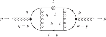
Figure 1: 3-loop ladder diagram containing a central local operator insertion.

Expanding the polynomial that appears raised to the $N$th power, one can see that the $w_{1}$- and $w_{2}$-integrals, can be written in terms of an Appell hypergeomteric function. After an appropriate analytic continuation, we end up with the following representation of the integral in terms of multiple sums,

$$\hat{I}_{1a} = \frac{\exp\left(-\frac{3}{2}\epsilon\gamma_{E}\right)\Gamma(2-3\epsilon/2)}{(N+1)(N+2)(N+3)}\sum_{m,n=0}^{\infty}\left\{\phantom{\sum_{t=1}^{N+2}\binom{N+3}{t}}\right.$$ (3)

$$\phantom{aaaaa}\sum_{t=1}^{N+2}\binom{N+3}{t}\frac{(t-\epsilon/2)_{m}(N+2+\epsilon/2)_{m+n}(N+3-t-\epsilon/2)_{n}}{(N+4-\epsilon)_{m+n}}$$

$$\phantom{aaaaa\sum_{t=1}^{N+2}}\times\Gamma{t,t-\epsilon/2,m+1+\epsilon/2,n+1+\epsilon/2,N+3-t,N+3-t-\epsilon/2\brack N+4-\epsilon,m+1,n+1,m+t+1+\epsilon/2,N+n-t+4+\epsilon/2}$$

$$\phantom{aaaa}-\sum_{s=1}^{N+3}\sum_{r=1}^{s-1}\binom{s}{r}\binom{N+3}{s}(-1)^{s}\frac{(r-\epsilon/2)_{m}(s-1+\epsilon/2)_{m+n}(s-r-\epsilon/2)_{n}}{(s+1-\epsilon)_{m+n}}$$

$$\left.\phantom{aaaa-\sum_{s=1}^{N+3}\sum_{r=1}^{s-1}}\times\Gamma{r,r-\epsilon/2,s-r,m+1+\epsilon/2,n+1+\epsilon/2,s-r-\epsilon/2\brack m+1,n+1,m+r+1+\epsilon/2,s-r+n+1+\epsilon/2,s+1-\epsilon}\right\}\,.$$

We can now expand in $\varepsilon$, and the resulting multiple sums can then be performed using the package Sigma. The result for this and other integrals can be written in terms of harmonic sums $S_{\vec{a}}$ [23] and their generalizations $S_{\vec{a}}(\vec{\xi};N)$ [24, 25] :

$$S_{b,\vec{a}}(N) = \sum_{k=1}^{N}\frac{{\rm sign}(b)^{k}}{k^{|b|}}S_{\vec{a}}(k),\quad S_{\emptyset}(k)=1$$

$$S_{b,\vec{a}}(\eta,\vec{\xi};N) = \sum_{k=1}^{N}\frac{\eta^{k}}{k^{b}}S_{\vec{a}}(\vec{\xi};k),\quad S_{\emptyset}=1,\quad\eta,\xi\in\mathbb{R}\,.$$ (4)

Omitting the explicit dependence of the harmonic sums on $N$, we obtain

$$\hat{I}_{1a} = -\frac{4(N+1)S_{1}+4}{(N+1)^{2}(N+2)}\zeta_{3}+\frac{2S_{2,1,1}}{(N+2)(N+3)}+\frac{1}{(N+1)(N+2)(N+3)}\left\{-2(3N+5)S_{3,1}-\frac{S_{1}^{4}}{4}\right.$$ (5)

$$+\frac{4(N+1)S_{1}-4N}{N+1}S_{2,1}+2\left[(2N+3)S_{1}+\frac{5N+6}{N+1}\right]S_{3}+\frac{2(3N+5)S_{1}^{2}}{(N+1)(N+2)}+\frac{9+4N}{4}S_{2}^{2}$$

$$+\left[2\frac{7N+11}{(N+1)(N+2)}+\frac{5N}{N+1}S_{1}-\frac{5}{2}S_{1}^{2}\right]S_{2}+\frac{N}{N+1}S_{1}^{3}+\frac{4(2N+3)}{(N+1)^{2}(N+2)}S_{1}$$

$$-\frac{1}{2}(2N+3)S_{4}\left.+8\frac{2N+3}{(N+1)^{3}(N+2)}\right\}~{}.$$

This result was checked using MATAD [27] for the fixed moments $N=1\ldots 10$. Other, more involved, integrals calculated in a similar way were given in Ref. [14].

The second method we have used to compute the integrals is based on an algorithm originally proposed in [19]. It is applicable when the integral turns out to be finite, even in case for local operator insertions for a fixed integer value of the Mellin variable $N$. We have generalized this method to the case allowing for one non-vanishing fermion mass and local operator insertions in order to find the general $N$-representations for convergent $3$-loop topologies. We work in the $\alpha$-representation and obtain integrals of the form

$$I_{4}(N)=\int\cdots\int d\alpha_{1}~{}d\alpha_{2}~{}d\alpha_{3}~{}d\alpha_{4}~{}d\alpha_{5}~{}d\alpha_{6}~{}d\alpha_{7}~{}d\alpha_{8}~{}\frac{T}{U^{2}V^{2}}\delta\left(1-\sum_{i}\alpha_{i}\right)\,.$$ (6)

The corresponding graph polynomials of a graph $G$ are given by

•   $U=\sum_{T}\prod_{l\notin T}\alpha_{l}$, where $T$ denotes the spanning trees of $G$.

•   $V=\sum_{l\in massive}\alpha_{l}$.

•   Dodgson polynomials [28] $T$ arise from the operator insertions. The form of these poly-      nomials will depend on the specific operator insertion we are considering.

The integrals given by (6) are projective integrals, where one $\alpha$-parameter may be set to one eliminating the $\delta$–distribution. The operators sit on on-shell diagrams which obey specific symmetries. These are generally not obeyed by the operator insertion. The Feynman parameter integrals are now performed in terms of hyperlogarithms [19] $L(\overrightarrow{w},z):\mathbb{C}\backslash\Sigma\rightarrow\mathbb{C}$, where

•   $\Sigma=\{\sigma_{0},\sigma_{1},...,\sigma_{N}\}$ are distinct points in $\mathbb{C}$ which may contain integration variables.

•   $\overrightarrow{w}$ is a word over the alphabet $\mathfrak{A}=\{a_{0},a_{1},...,a_{N}\}$, where each letter $a_{i}$ corresponds to a      point $\sigma_{i}$.

$L\left({\overrightarrow{w}},z\right)$ is uniquely defined by the following properties :

$$L\left(\{\},z\right)=1,~{}~{}\text{and}~{}~{}L\left({0^{n}},z,\right)=\frac{1}{n!}\log^{n}(z)~{}~{}\text{for}~{}~{}n\geq 1$$

$$\frac{\partial}{\partial z}L\left(\left\{a_{i}\overrightarrow{w}\right\},z\right)=\frac{1}{z-\sigma_{i}}L\left({\overrightarrow{w}},z\right)~{}~{}\text{for}~{}~{}z\in\mathbb{C}\backslash\Sigma$$

$$\text{If}~{}~{}\overrightarrow{w}~{}~{}\text{is not of the form}~{}~{}w=(0,0,\cdots,0),~{}~{}\text{then}\lim_{z\rightarrow 0}L\left({\overrightarrow{w}},z\right)=0.$$ (7)

For example, $L\left(a_{i},z\right)=\log(z-\sigma_{i})-\log(\sigma_{i})$.

The hyperlogarithms satisfy shuffle relations, e.g.

$$L\left(\{a_{1},a_{2}\},z\right)L\left(\{a_{3}\},z\right)=L\left(\{a_{3},a_{1},a_{2}\},z\right)+L\left(\{a_{1},a_{3},a_{2}\},z\right)+L\left(\{a_{1},a_{2},a_{3}\},z\right)~{}.$$ (8)

The points to which the indices $a_{i}$ correspond may contain further integration variables. Using these properties after partial fractioning and integration by parts, one can express any primitive for expressions consisting of rational and hyperlogarithmic functions in terms of different hyperlogarithmic functions. These primitives have to be evaluated at the respective integration limits. Due to the operator-insertions leading to power-type functions, the integrals do not fit directly into the framework of the algorithm for general values of $N$. In order to obtain the corresponding extension a generating function is constructed by the mapping,

$$p\left(\alpha_{1},\cdots,\alpha_{n}\right)^{N}\rightarrow\sum_{k=0}^{\infty}x^{k}p\left(\alpha_{1},\cdots,\alpha_{n}\right)^{k}=\frac{1}{1-x~{}p\left(\alpha_{1},\cdots,\alpha_{n}\right)}~{}.$$ (9)

Figure 2: A 3-loop Benz diagram.

Performing the Feynman-parameter integrations then leads to an expression which contains hyperlogarithms $L_{w}$ in the variable $x$. Using this method, the scalar integral with all powers of propagators equal to one associated with the diagram shown in Fig. 2, corresponding to a Benz-type topology, yields

$$I(x) = \frac{1}{(1+N)(2+N)x}\Biggl{\{}\zeta_{3}\Bigl{[}{2}L\left(\{-1\},x\right)-2(-1+2x)L\left(\{1\},x\right)-4L\left(\{1,1\},x\right)\Bigr{]}$$

$$-{3}L\left(\{-1,0,0,1\},x\right)+{2}L\left(\{-1,0,1,1\},x\right)-{2xL\left(\{0,0,1,1\},x\right)}+{3xL\left(\{0,1,0,1\},x\right)}$$

$$-x{L\left(\{0,1,1,1\},x\right)}+{(-3+2x)L\left(\{1,0,0,1\},x\right)}+{2xL\left(\{1,0,1,1\},x\right)}-{L\left(\{1,0,1,1,1\},x\right)}$$

$$-{(5x-1)L\left(\{1,1,0,1\},x\right)}+x{L\left(\{1,1,1,1\},x\right)}-{2L\left(\{1,0,0,1,1\},x\right)}+{3L\left(\{1,0,1,0,1\},x\right)}$$

$$+{2L\left(\{1,1,0,0,1\},x\right)}+{2L\left(\{1,1,0,1,1\},x\right)}-{5L\left(\{1,1,1,0,1\},x\right)}+{L\left(\{1,1,1,1,1\},x\right)}\Biggr{\}}~{}.$$

Finally, the $N$th coefficient of this expression in $x$ has to be extracted analytically in order to undo the mapping (9). This is achieved using the GetMoments option of the package HarmonicSums [25]. One may also use guessing-methods to obtain the corresponding difference equation based on a huge number of moments, cf. [29]. For a more complicated graph with non-trivial argument structure in $x$ we were able to produce $\sim 1500$ moments [30]. One obtains from Eq. (10)

$$I(N) = \frac{1}{(N+1)(N+2)(N+3)}\Biggl{\{}\frac{648+1512N+1458N^{2}+744N^{3}+212N^{4}+32N^{5}+2N^{6}}{(1+N)^{3}(2+N)^{3}(3+N)^{3}}$$ (11)

$$-\frac{2\left(-1+(-1)^{N}+N+(-1)^{N}N\right)}{(1+N)}\zeta_{3}-(-1)^{N}S_{-3}-\frac{N}{6(1+N)}S_{1}^{3}+\frac{1}{24}S_{1}^{4}-\frac{1}{4}S_{4}$$

$$-\frac{\left(7+22N+10N^{2}\right)}{2(1+N)^{2}(2+N)}S_{2}-\frac{19}{8}S_{2}^{2}-\frac{1+4N+2N^{2}}{2(1+N)^{2}(2+N)}S_{1}^{2}+\frac{9}{4}S_{2}-\frac{(-9+4N)}{3(1+N)}S_{3}$$

$$-{2(-1)^{N}}S_{-2,1}+\frac{(-1+6N)}{(1+N)}S_{2,1}+\frac{54+207N+246N^{2}+130N^{3}+32N^{4}+3N^{5}}{(1+N)^{3}(2+N)^{2}(3+N)^{2}}S_{1}$$

$$+{4}\zeta_{3}S_{1}-\frac{(-2+7N)}{2(1+N)}S_{2}S_{1}+\frac{13}{3}S_{3}S_{1}-{7}S_{2,1}S_{1}-{7}S_{3,1}+{10}S_{2,1,1}\Biggr{\}}~{}.$$

Another example, where this technique has been applied, is shown in Fig. 3.

Figure 3: A second example of a 3-loop Benz topology.

In this case the result is

$$I(N) = \frac{1}{(N+1)(N+2)}\Biggl{\{}\frac{2\left(1-13(-1)^{N}+(-1)^{N}2^{3+N}+N-7(-1)^{N}N+3(-1)^{N}2^{1+N}N\right)}{(1+N)(2+N)}\zeta_{3}$$

$$+\frac{1}{(2+N)}S_{3}+\frac{(-1)^{N}}{2(2+N)}S_{1}^{3}-\frac{(-1)^{N}(3+2N)}{2(1+N)^{2}(2+N)}S_{2}+\frac{5(-1)^{N}}{2}S_{2}^{2}+\frac{2(-1)^{N}(3+N)}{(1+N)(2+N)}S_{2,1}$$

$$+\frac{(-1)^{N}(3+2N)}{2(1+N)^{2}(2+N)}S_{1}^{2}-\frac{(-1)^{N}}{2}S_{2}S_{1}^{2}+\frac{3(-1)^{N}(4+3N)}{(1+N)(2+N)}S_{3}+3(-1)^{N}S_{4}+\frac{2}{(2+N)}S_{-2,1}$$

$$-{12(-1)^{N}}S_{1}\zeta_{3}+\frac{(-1)^{N}(5+7N)}{2(1+N)(2+N)}S_{1}S_{2}+{3(-1)^{N}}S_{1}S_{3}+{4(-1)^{N}}S_{2,1}S_{1}-{4(-1)^{N}}S_{3,1}$$

$$-\frac{4\left((-1)^{N}2^{2+N}-3(-2)^{N}N+3(-1)^{N}2^{1+N}N\right)}{(1+N)(2+N)}S_{1,2}\left(\frac{1}{2},1\right)-{5(-1)^{N}}S_{2,1,1}$$

$$+{2(-1)^{N}}\zeta_{3}S_{1}\left(2\right)+\frac{2\left(-(-1)^{N}2^{2+N}-13(-2)^{N}N+5(-1)^{N}2^{1+N}N\right)}{(1+N)(2+N)}S_{1,1,1}\left(\frac{1}{2},1,1\right)$$

$$-{2(-1)^{N}}S_{1,1,2}\left(2,\frac{1}{2},1\right)-{(-1)^{N}}S_{1,1,1,1}\left(2,\frac{1}{2},1,1\right)\Biggr{\}}\,.$$ (12)

Notice the presence of generalized harmonic sums and highly divergent factors in the limit $N\rightarrow\infty$, such as $2^{N}$. It can be shown, however, that the complete expression is convergent in this limit and possesses a well-defined asymptotic expansion for $N\rightarrow\infty$. In general neither the representation in individual nested sums or by iterated integrals shows this property, but a corresponding combination of terms does.

We calculated the contributions of $O(n_{f}T_{F}^{2}C_{A,F})$ to all massive OMEs completely [12, 13]. Furthermore, first systematic results were obtained for the case of graphs containing two massive fermion lines with $m_{1}=m_{2}$. A typical graph is shown in Fig. 4 in the gluonic case.

Figure 4: A 3-loop graph containing two massive fermion lines $m_{1}=m_{2}$ and an operator insertion.

One obtains

$$I= \frac{1}{105\varepsilon^{2}}+\frac{1}{\varepsilon}\Biggl{[}\frac{74N^{3}-455N^{2}+381N-210}{44100(N-1)N(N+1)}-\frac{1}{210}S_{1}(N)\Biggr{]}$$

$$+\frac{8903N^{3}+39537N^{2}-114440N+36576}{2822400(N+1)(2N-3)(2N-1)}S_{1}(N)$$

$$+\frac{P_{1}}{148176000(N-1)^{2}N^{2}(N+1)^{2}(2N-3)(2N-1)}+\frac{1}{840}\Bigl{(}S_{1}(N)^{2}+S_{2}(N)+3\zeta_{2}\Bigr{)}$$

$$+\frac{2^{-2N-9}(N-1)N(5N-6)}{3(2N-3)(2N-1)}\binom{2N}{N}\Biggl{(}-7\zeta_{3}-\sum_{j=1}^{N}\frac{4^{j}}{\binom{2j}{j}j^{3}}+\sum_{j=1}^{N}\frac{4^{j}S_{1}(j)}{\binom{2j}{j}j^{2}}\Biggr{)}~{},$$ (13)

$$P_{1}= 1795487N^{8}-7087789N^{7}+10654130N^{6}-5797102N^{5}+6828839N^{4}-16594069N^{3}$$

$$+9651144N^{2}+902160N-1058400~{}.$$ (14)

Integrals of this type usually contain finite binomial and inverse binomial sums, which even may be nested.

In conclusion, we have seen that the methods shown here allow us to obtain analytic expressions at general values of $N$ for 3–loop integrals contributing to the massive OMEs which could not be obtained by other methods before. We continue working on the set of integrals that we need in order to obtain all necessary operator matrix elements. In particular, we are studying the possibility also to extend the method of hyperlogarithms. Application of these methods to the more complicated case of non-planar integrals are underway. The package Sigma and related packages are continuously being upgraded to be able to meet the challenges that keep arising in this endeavor.

Acknowledgment.  We would like to thank F. Brown for discussions. The Feynman diagrams have been drawn using Axodraw. This work has been supported in part by DFG Sonderforschungsbereich Transregio 9, Computergestützte Theoretische Teilchenphysik, by the Austrian Science Fund (FWF) grant P203477-N18, by the EU Network LHCPHENOnet PITN-GA-2010-264564, and ERC Starting Grant PAGAP FP7-257638.

References

• [1] M. Buza, Y. Matiounine, J. Smith, R. Migneron and W. L. van Neerven, Nucl. Phys. B 472 (1996) 611 [hep-ph/9601302].
• [2] I. Bierenbaum, J. Blümlein and S. Klein, Nucl. Phys. B 820 (2009) 417 [arXiv:0904.3563 [hep-ph]].
• [3] E. Witten, Nucl. Phys. B 104 (1976) 445;
J. Babcock, D. W. Sivers and S. Wolfram, Phys. Rev. D 18 (1978) 162;
J. P. Leveille and T. J. Weiler, Nucl. Phys. B 147 (1979) 147;
M. Glück, E. Hoffmann and E. Reya, Z. Phys. C 13 (1982) 119.
• [4] E. Laenen, S. Riemersma, J. Smith and W. L. van Neerven, Nucl. Phys. B 392 (1993) 162; 229;
S. Riemersma, J. Smith and W. L. van Neerven, Phys. Lett. B 347 (1995) 143 [hep-ph/9411431].
• [5] S. I. Alekhin and J. Blümlein, Phys. Lett. B 594 (2004) 299 [hep-ph/0404034].
• [6] J. A. M. Vermaseren, A. Vogt and S. Moch, Nucl. Phys. B 724 (2005) 3 [hep-ph/0504242].
• [7] J. Blümlein, The Theory of Deeply Inelastic Scattering, arXiv:1208.6087 [hep-ph].
• [8] J. Blümlein and W. L. van Neerven, Phys. Lett. B 450 (1999) 417 [hep-ph/9811351].
• [9] J. Blümlein, A. De Freitas, W. L. van Neerven and S. Klein, Nucl. Phys. B 755 (2006) 272 [hep-ph/0608024].
• [10] J. Ablinger, J. Blümlein, S. Klein, C. Schneider and F. Wißbrock, arXiv:1106.5937 [hep-ph].
• [11] J. Ablinger, J. Blümlein, A. Hasselhuhn, S. Klein, C. Schneider and F. Wißbrock, PoS (RADCOR2011) 031, arXiv:1202.2700 [hep-ph].
• [12] J. Ablinger, J. Blümlein, S. Klein, C. Schneider and F. Wißbrock, Nucl. Phys. B 844 (2011) 26 [arXiv:1008.3347 [hep-ph]].
• [13] J. Blümlein, A. Hasselhuhn, S. Klein and C. Schneider, Nucl. Phys. B 866 (2013) 196 [arXiv:1205.4184 [hep-ph]].
• [14] J. Ablinger, J. Blümlein, A. Hasselhuhn, S. Klein, C. Schneider and F. Wißbrock, Nucl. Phys. B 864 (2012) 52 [arXiv:1206.2252 [hep-ph]].
• [15] I. Bierenbaum, J. Blümlein and S. Klein, Nucl. Phys. B 780 (2007) 40 [hep-ph/0703285 [HEP-PH]]; Phys. Lett. B 672 (2009) 401 [arXiv:0901.0669 [hep-ph]];
I. Bierenbaum, J. Blümlein, S. Klein and C. Schneider, Nucl. Phys. B 803 (2008) 1 [arXiv:0803.0273 [hep-ph]].
• [16] J. Blümlein, A. De Freitas and W. van Neerven, Nucl. Phys. B 855 (2012) 508 [arXiv:1107.4638 [hep-ph]].
• [17] P. Nogueira, J. Comput. Phys.  105 (1993) 279.
• [18] C. Schneider, J. Symbolic Comput. 43 (2008) 611 [arXiv:0808.2543]; Ann. Comb. 9 (2005) 75; J. Differ. Equations Appl. 11 (2005) 799; Ann. Comb. 14 (2010) [arXiv:0808.2596]; Clay Mathematics Proceedings 12 (2010) 285; Sem. Lothar. Combin. 56 (2007) 1, Article B56b, Habilitationsschrift JKU Linz (2007) and references therein;
J. Ablinger, J. Blümlein, S. Klein, C. Schneider, Nucl. Phys. (Proc. Suppl.) 205-206 (2010) 110 [arXiv:1006.4797].
• [19] F. Brown, Commun. Math. Phys.  287 (2009) 925 [arXiv:0804.1660].
• [20] V. A. Smirnov, Phys. Lett. B 460 (1999) 397 [hep-ph/9905323];
I. Bierenbaum, J. Blümlein and S. Klein, Phys. Lett. B 648 (2007) 195 [hep-ph/0702265]; Nucl. Phys. Proc. Suppl.  160 (2006) 85 [hep-ph/0607300].
• [21] K. G. Chetyrkin, A. L. Kataev and F. V. Tkachov, Nucl. Phys.  B 174 (1980) 345.
• [22] J. Blümlein, Comput. Phys. Commun.  180 (2009) 2218 [arXiv:0901.3106 [hep-ph]];
J. Blümlein, S. Klein, C. Schneider and F. Stan, J. Symbolic Comput. 47 (2012) 1267-1289 [arXiv:1011.2656 [cs.SC]].
• [23] J. Blümlein and S. Kurth, Phys. Rev. D 60 (1999) 014018 [hep-ph/9810241];
J. A. M. Vermaseren, Int. J. Mod. Phys. A 14 (1999) 2037 [hep-ph/9806280].
• [24] S. Moch, P. Uwer and S. Weinzierl, J. Math. Phys.  43 (2002) 3363 [hep-ph/0110083];
• [25] J. Ablinger, J. Blümlein and C. Schneider, DESY 12–210;
J. Ablinger, Computer Algebra Algorithms for Special Functions in Particle Physics, J. Kepler University Linz. PhD Thesis. April 2012;
http://www.risc.jku.at/research/combinat/software/
• [26] J. Ablinger, J. Blümlein and C. Schneider, J. Math. Phys.  52 (2011) 102301 [arXiv:1105.6063 [math-ph]].
• [27] M. Steinhauser, Comput. Phys. Commun.  134 (2001) 335 [hep-ph/0009029].
• [28] C. Bogner and S. Weinzierl, Int. J. Mod. Phys. A 25 (2010) 2585 [arXiv:1002.3458 [hep-ph]];
F. Brown and O. Schnetz, arXiv:1006.4064 [math.AG].
• [29] J. Blümlein, M. Kauers, S. Klein and C. Schneider, Comput. Phys. Commun.  180 (2009) 2143 [arXiv:0902.4091 [hep-ph]].
• [30] J. Ablinger, J. Blümlein, C. Schneider and F. Wißbrock, in preparation.
• [31] J. A. M. Vermaseren, Axodraw, Comput. Phys. Commun.  83 (1994) 45.