Modelling page-view dynamics on Wikipedia

Abstract

We introduce a model for predicting page-view dynamics of promoted content. The regularity of the content promotion process on Wikipedia provides excellent experimental conditions which favour detailed modelling. We show that the popularity of an article featured on Wikipedia’s main page decays exponentially in time if the circadian cycles of the users are taken into account. Our model can be explained as the result of individual Poisson processes and is validated through empirical measurements. It provides a simpler explanation for the evolution of content popularity than previous studies.

1 Introduction

The social media boom gave a birth to a wide range of studies about online traces generated by Internet users. One of the important research targets addressed by these studies is the analysis and prediction of the dynamics of content popularity. Historically, most of these scientific works focused on the analysis of content generated on blogging [1, 4], later microblogging [5], video-sharing [12] and news-sharing platforms [2]. However, in many cases the studies reflect only the behaviour of registered users or focus on a website of interest only for a specific community. Here we analyse instead a website of general interest and address the problem of understanding online usage and popularity patterns through a large-scale analysis of the behaviour of the visitors of Wikipedia, the sixth most visited website.

Wikipedia has an estimated number of 365 million monthly readers worldwide [14]. Although many studies analysed editing and commenting activity on Wikipedia, e.g. [3, 7, 11, 16], there are not many quantitative works focusing on the Wikipedia usage by the Internet users. A few studies explore Wikipedia views as an information source in order to detect and predict events in real world. Osborne et al. [8] used a stream of Wikipedia page-views to improve the quality of discovered events in Twitter, and Mestyán et al. [6] predicted the popularity of a movie by measuring the activity level of editors and viewers of the corresponding Wikipedia entry. Finally, two studies [9, 10] analysed how the Wikipedia traffic data is influenced by external and internal events.

The goal of this work is to examine the temporal evolution of the popularity of promoted content on Wikipedia. The competition for attention between numerous amounts and different types of content makes it difficult to find sufficiently regular and repetitive conditions which allow to predict how much attention will be devoted from Internet users to a piece of content. Some studies [12, 13, 15] tried to address this question by analysing media-sharing platforms such as Digg or Youtube. These platforms rank and categorise content based on previous popularity and user votes, which leads to rich-get-richer bias in the number of views and in the duration of the promotion time.

The concept of content promotion on Wikipedia is distinctively different. Similar to many online platforms, on Wikipedia some of the articles get promoted to the Main page. Promoted articles on Wikipedia are generated and managed through online collaboration and a fixed number is shown to the online audience during a fixed amount of time. This predefined exposure duration together with the fact that only one article is promoted per day makes the Wikipedia promotion mechanism unique in its regularity compared to other large and popular social media platforms. It provides thus excellent experimental conditions.

Figure 1: The promoted article on the English Wikipedia’s Main page of December 20, 2012.

Figure 1 presents an example of the Main page of the English Wikipedia. Every Wikipedia user (although preference is given to the articles’ primary editors) can nominate articles with certain characteristics (featured articles) to the pool of possible future promoted articles on a specific page. We refer to the article placed under the headline “From today’s featured article” as promoted. Every day, at 00h(UTC), a new promoted article is placed on the Main page together with links to the three articles promoted during the previous three days (see “Recently featured” at the bottom left of Figure 1). The “today’s promoted” articles are also sent by e-mail to subscribers.

2 Dataset

We retrieved the page-view values from a database provided by Wikimedia. This database contains one file per hour, listing the total number of views to a page during that hour, provided it received at least one view. We extracted the page-view data between December 9, 2007 at 18h(UTC) and March 31, 2010 23h(UTC), for a total of 844 days. Note that this database is not entirely complete: for some hours there is missing data or there is more than one entry for a single article. For the latter we just sum these entries. Finally, we assume that views to articles which come through redirects are also registered in the data of the target page.

For comparison with the general access pattern to Wikipedia we also used the Wikipedia dump from March 12, 2010 and extracted the view data of all Wikipedia articles which received at least one comment until this date in their discussion page. This led to 871 395 articles which accumulated $32\cdot 10^{9}$ views in total, i.e. on average $38\cdot 10^{6}$ per day.

3 Page-view Statistics

We describe here the hourly and daily number of page-views on the English Wikipedia and analyse then the popularity of a promoted article during the promotion period.

3.1 Circadian and weekly patterns

In Figure 2 we depict the number of visits per hour to the English Wikipedia in general and also to its Main page averaged by weeks (left) and by days (middle sub-figure). The visits of the English Wikipedia vary between $1.4\cdot 10^{6}$ and $1.8\cdot 10^{6}$ with an average of $1.6\cdot 10^{6}$ page-views per hour. For the Main page popularity we find on average $2.5\cdot 10^{5}$ visitors per hour. The Main page pattern is similar to the overall weekly pattern. Both slightly decrease during weekends.

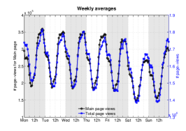
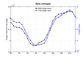
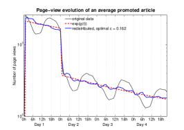
Figure 2: Temporal patterns of the Wikipedia views per hour in total and for its Main page (left, centre) and the average number of views of a promoted article arranged by different time scales (right).

Figure 2 (middle sub-figure) depicts the circadian patterns of the Wikipedia page-views. We observe the lowest activity between 07h and 10h(UTC) corresponding to the night hours in the US. Similar circadian patterns but for editing activity on the English Wikipedia were observed in [16].

3.2 Promoted articles

In the previous section we have analysed the temporal views of Wikipedia articles and the Wikipedia’s main page in general. In the rest of this work we will focus on the page-view data for the promoted articles only. Recall that in Wikipedia an article gets promoted for a predefined period of 1+3 days (96 hours), which we call the exposure duration in analogy to [13]. We restrict our analysis and predictions only to these article exposure durations.

We select all the articles promoted in the time-span from January 1, 2008 to March 31, 2010, which have complete page-view data, i.e. we obtained the number of views for every hour in their exposure duration. We omit the articles of Barack Obama and John McCain, promoted both on November 4, 2008. They show completely different dynamics compared to the average article and would influence some of the results reported below as they have the largest number of views during the second day of exposure (once the presidential elections were decided). Thus, in total we use 684 promoted articles in this study.

By popularity of a promoted article we mean the number of views this article receives during the exposure duration. The right sub-figure of Figure 2 depicts the average number of views $v_{t}$ a promoted article attracts during the $t=1,\ldots,96$ hours of exposure. The exposure period of a promoted article in Wikipedia can be divided into four stages. At the first stage, during the first hour after a page gets promoted, we witness a huge increase in the article’s popularity. This value $v_{1}$ is the largest for the average promoted article. The second stage contains the remaining hours of the first day of the promotion. The third stage is characterised by the sharp decay occurring after the original article gets replaced by the new one. Finally, the last stage contains the view dynamics during the 3 days of being promoted in “Recently featured”. Using this stage-representation, we construct $g(t)$ (dashed red line in Figure 2, right) as a piecewise-linear approximation of $\log(v_{t})$.

3.3 Circadian patterns correction

Comparing the approximation $g(t)$ and the promoted article popularity $v_{t}$ we notice that the main differences are caused by the circadian patterns of Wikipedia views. To remove these variations we use a new time scale in which every hour is measured in the number of views rather than in minutes. This approach was introduced in [12] for the popularity of Digg stories. We modify the original idea by removing a constant fraction $c$ of the traffic data to emphasise the circadian patterns even more.

Formally, we denote as $m(t)$ the average number of Main page views for a given hour $t=1,\dots,24$. We define a new redistribution parameter $T^{*}$ as follows:

$$T^{*}=\sum_{t=1}^{24}m^{*}(t)=\sum_{t=1}^{24}[m(t)-c\min_{t}m(t)],$$

where $c=\mbox{arg}\min\left[\sum_{t^{*}=0}^{95}\left(\log\left(v_{t^{*}}\right)-g(t^{*})\right)^{2}\right]$ and $v_{t^{*}}$ (depends on $c$) is the number of views of an average promoted page at time $t^{*}$ in the new time scale defined by $T^{*}$. We find that $c=0.162$ is the optimal value for “decycling” based on the Main page views. In other words one needs to remove approximately 16% of the minimum of the hourly traffic of the Wikipedia Main page to make an optimal correction of the circadian patterns. A new hour $t^{*}$ is therefore the time interval which takes the Main page to accumulate from $\frac{t^{*}-1}{24}T^{*}$ to $\frac{t^{*}}{24}T^{*}$.

In the rest of the paper we refer to the new time scale $t^{*}$ as redistributed time scale. The blue line in Figure 2 (right) depicts the average number of views $v_{t^{*}}$ of the promoted articles in the redistributed time scale. We observe the log-linear decreasing trend of the promoted article. popularity.

4 Model

Based on the average view behaviour, i.e. the average number of views per hour over all promoted articles, we propose a model which describes the traffic dynamics of a selected promoted article during its exposure duration. This model is defined by two parameters: a constant interest-decay factor for all days of the promotion and negative jump of the popularity after the first day of exposure. The number of views $v_{1}$ a selected article receives during the first hour of the promotion is used as the only input value of the model.

4.1 Model definition

The definition of the model is inspired by the shape of the page-view behaviour pattern, or more exactly by the normalised number of views per time unit $w_{t^{*}}=v_{t^{*}}/v_{1^{*}}$ in rescaled time (with the circadian cycle removed).

Based on the log-linear fit of $w_{t^{*}}$ and using $w_{1^{*}}=1$ we define the model as:

$$\hat{w}_{1^{*}} = 1$$

$$\hat{w}_{t^{*}} = \beta_{t^{*}}\cdot\hat{w}_{t^{*}-1}\mbox{ for }t^{*}=2,\dots,95$$

Previously, we have described the four stages of the exposure life of a promoted article on Wikipedia. Using these definitions we set a temporal factor $\beta_{t^{*}}$ as $\beta_{t^{*}}={\gamma}$ for $t^{*}=25$ and $\beta_{t^{*}}={\beta}$ for other $t^{*}$’s, i.e. for $2\leq t^{*}\leq 24$ and $26\leq t^{*}\leq 95$. The constant factor $\beta$ models the decay of the number of page-views in a typical hour of the exposure duration, i.e. while the article is promoted on the Main page. The factor $\gamma$ states for the negative jump in the number of views after the promoted article gets moved to “Recently featured” position. Thus, we model the shape of the article popularity by stage: the first stage of the promoted article is characterised by $\hat{w}_{1^{*}}$, the second by the interest-decay factor $\beta$, the third by $\gamma$, and the fourth again by the same factor $\beta$. To summarise, we model the normalised number of views of the promoted article during the $t^{*}$-th redistributed hour as follows:

$$\hat{w}_{t^{*}}=\left\{\begin{array}[]{rcr}{\beta^{t^{*}-1}}&\mbox{for}&2\leq t^{*}\leq 24;\\ {\gamma\beta^{t^{*}-2}}&\mbox{for}&25\leq t^{*}\leq 95.\end{array}\right.$$

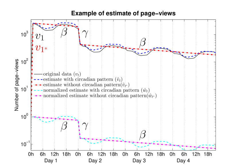
Figure 3: Visualisation of the popularity model for promoted articles.

Finally, we use the reverse time-redistribution to find $\hat{w}_{t},$ i.e. the corresponding number for $\hat{w}_{t^{*}}$ but in the original time scale. We define the number of views of the promoted article during $t$-th hour as

$$\hat{v}_{t}=v_{1^{*}}\cdot\hat{w}_{t},$$

where $v_{1}$ and $v_{1^{*}}=v_{1}/\hat{w}_{1}$ are the numbers of views of the promoted article after the first hour of exposure in the original and redistributed time scales.

In Figure 3 we draw a visual explanation of the model. The dashed-dotted lines in magenta correspond to the model curve $\hat{w}_{t^{*}}$ and the cyan dashed curve to its transformation $\hat{w}_{t}$ into the real timescale. The multiplication of $\hat{w}_{t}$ with $v_{1}$ leads to the model approximation $\hat{v}_{t}$ (blue dashed curve) of the original data $v_{t}$ (black curve). Figure 3 also depicts the rescaled model $v_{t*}$ in the redistributed time scale as dashed dotted line in red.

The introduced model uses only the number of views during the first hour of the exposure period $v_{1}$ as an input parameter. In Figure 4 we plot the histogram for $v_{1}$’s in our dataset together with the log-normal fit ($\mu=7.63$ and $\sigma=0.71$). We have also investigated whether the values of $v_{1}$ correlate with the page-views of the corresponding articles before being promoted. No such correlations were found.

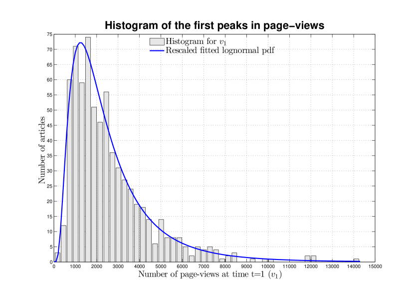
Figure 4: Histogram of occurring values for $v_{1}$.

4.2 Model interpretation

The model can be explained as the consequence of individual Poisson processes at the user level. We assume that the users visit a promoted article only once and thus, given that in a Poisson process the probability of the first arrival time $T_{1}$ being larger than $t$ is

$$\mbox{P}(t<T_{1})=\exp(-\lambda t)=\beta^{t},$$

we can find that

$$\mbox{P}(t-1<T_{1}\leq t)=\mbox{P}(t-1<T_{1})-\mbox{P}(t<T_{1})=\beta^{t-1}(1-\beta).$$

The above formula corresponds to the likelihood that an individual user visits a promoted article during the $t$-th hour of exposure on the Main page. It is, apart from the constant factor $(1-\beta)$, identical to the decay factor $\beta^{t-1}$ of our model. This constant factor can be neglected as part of a normalising constant. The parameter $\gamma$ corresponds to the decrease in the likelihood of visiting an article after it has passed to the “Recently featured” section.

The actual number of page-views is determined by how many users get curious about an article and visit it after they observe a link to it on the Main page (or receive it via an e-mail subscription). We model the time distribution of these page-views, which is governed by individual Poisson processes with rate $\lambda=-\ln(\beta)$.

4.3 Parameter Estimation

We estimate the model’s parameters $\beta$ and $\gamma$ by using page-view data of the promoted articles on the English Wikipedia. To investigate the stability of the parameter estimation we apply the estimation algorithms for two sets of promoted articles. The first set $S_{a}$ contains all 684 articles and the second set $S_{1}$ the first 100 promoted articles by date of promotion. We use $S_{a}$ to describe the general view dynamics for promoted content on Wikipedia and $S_{1}$ to predict the popularity of the 584 articles promoted afterwards.

We denote as $\hat{v}_{t^{*}}(\beta,\gamma)$ the predicted number of views for given values of $\beta$ and $\gamma$ at redistributed time $t^{*}$, and as $v_{t^{*}}$ the actual number of page-views at time $t^{*}$ for some promoted article $s\in S,$ where $S$ is either $S_{a}$ or $S_{1}$. Then, we calculate parameters $\beta$ and $\gamma$ that minimise the error:

$$\left\{\beta,\gamma\right\}=\mbox{arg}\min\sum_{s\in S}\left[\sum_{t^{*}=1}^{95}\left[\log(\hat{v}_{t^{*}}(\beta,\gamma))-\log(v_{t^{*}})\right]^{2}\right]$$ (1)

This yields to $\beta=0.9874$ and $\gamma=0.2319$ for $S_{a}s$ and to $\beta=0.9877$ and $\gamma=0.2618$ for $S_{1}$. We observe that the value of $\beta$ is very similar for the two set while there is a small difference for $\gamma$.

To investigate this further we drop the assumption that $\gamma$ can be modelled as a constant factor for all articles and look at the $\gamma$ parameters at the individual article level. Since $\gamma$ encodes the negative jump in the decay of user interest after the first day of the exposure, we suggest that it should be correlated with the overall popularity of the promoted article. To this end, we compared the values of $\gamma$ with the total number of views a promoted article receives during one day before the promotion date but found no correlation between them. Instead, we propose to define $\gamma$ as function of the initial popularity $v_{1}$. We first find that $\log(v_{1})$ and $\log(\gamma)$ are negatively correlated (Pearson’s correlation coefficient is $-0.29$ for $S_{a}$ and $-0.25$ for $S_{1}$), which is also indicated in Figure 5. Then, we derive a log-linear function for $\gamma$:

$$\gamma=C\cdot v_{1}^{m},$$

based on the observations $\{\log(v_{1}),\log(\gamma)\}$ for the articles from set $S$, where $S$ is again either $S_{a}$ or $S_{1}$. We rewrite the last equation in the following form:

$$\log(\gamma)=h(v_{1})=m\cdot\log(v_{1})+\log(C).$$ (2)

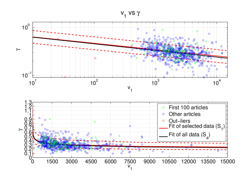
Figure 5: Relations between $\gamma$ and $v_{1}$. The dashed red lines indicate the interval $[h(v_{1})-\sigma,h(v_{1})+\sigma]$.

Using the set $S_{a}$ we obtain $m=-0.138$ and $C=0.863$ for all articles. We note that for estimation of parameters $m$ and $C$ we omit the outliers indicated as red squares in Figure 5. We also perform the fitting for (2) on $S_{1}$ and obtain $m=-0.132$ and $C=0.862$. Note that, although the initial estimates for $\gamma$ were slightly different for $S_{a}$ and $S_{1}$, the parameters of $h(v_{1})$ are not. This can be also observed in the nearly overlapping linear fits in Figure 5. The reason for this greater stability is that we now focus only on the size of the drop and not on the effect of the choice of $\gamma$ on the minimisation of the model error in the subsequent days as Equation (1) would do.

Comparing the estimated values for $\log(\gamma)$ with $h(v_{1})$, we find that $\log(\gamma)\sim\mathcal{N}(h(v_{1}),\sigma^{2})$. Therefore, we can derive an interval in which the decay factor would lie with a given probability. We use $[h(v_{1})-\sigma,h(v_{1})+\sigma]$ as this interval, indicated by the dashed lines in Figure 5.

Back to the model, we can now calculate $\hat{w}_{t^{*}}$ at time $t^{*}$ as follows:

$$\hat{w}_{t^{*}}=\left\{\begin{array}[]{rcr}{\beta^{t^{*}-1}}&\mbox{for}&2\leq t^{*}\leq 24;\\ {C\cdot v_{1}^{m}\cdot\beta^{t^{*}-2}}&\mbox{for}&25\leq t^{*}\leq 95;\end{array}\right.$$ (3)

and then use the reverse time-redistribution to find $\hat{w}_{t}$. Using $\hat{w}_{t}$ and

$$\hat{v}_{t}=\frac{v_{1}}{\hat{w}_{1}}\cdot\hat{w}_{t}$$ (4)

we can obtain the estimated hourly progression $\hat{v}_{t}$ of the page-views for $t=2,\ldots,95$.

5 Popularity Prediction

As explained in the previous section, we use the first 100 promoted articles (ordered by date of exposure) to learn the model parameters and predict the popularity of the 584 Wikipedia articles of our dataset promoted a posteriori. Thus, for each of these articles we take the article’s popularity after the first hour $v_{1}$ and use Eq. (3) and (4) with the parameters $\beta=0.9877$ and $\gamma$ ($m=-0.132$, $C=0.862$) of $S_{1}$.

As we will discuss below for most of the promoted articles we are able to obtain a good prediction for the page-view dynamics during the first day of exposure. However, for the remaining days the number of actual page-views $v_{t}$ does not always lie within the predicted interval $[h(v_{1})-\sigma,h(v_{1})+\sigma]$ for $t=25,\ldots,95,$ as we see in Figure 6. Thus, although in the 25-th hour we correctly predict the page popularity for 50% of the articles, in general we observe a lower percentage of correct predictions. This is caused by underestimating the decline of interest (or an overestimation of $\gamma$) by our model and can be improved by introducing the input parameter $v_{25}$, i.e. the value of the promoted page popularity right after it is moved to the “Recently featured” section, into our model.

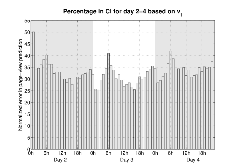
Figure 6: Percentage of values $v_{t}$ in predicted interval for $t=25,\ldots,95$.

Adjusting the prediction during the first hour of the second day of the promotion with $v_{25}$ leads us to the following description of the model:

$$\hat{w}_{t^{*}}=\left\{\begin{array}[]{lcr}{\beta^{t^{*}-1}}&\mbox{for}&1\leq t^{*}\leq 24;\\ {\beta^{t^{*}-25}}&\mbox{for}&25\leq t^{*}\leq 95.\end{array}\right.$$

Here we use again the reverse time-redistribution to find $\hat{w}_{t}$ to obtain the predicted hourly page-views progression $\hat{v}_{t}$, for $t=2,\ldots,95$ by calculating

$$\hat{v}_{t}=\left\{\begin{array}[]{rcr}\frac{v_{1}}{\hat{w}_{1}}\cdot\hat{w}_{t}&\mbox{for}&1\leq t\leq 24;\\ \frac{v_{25}}{\hat{w}_{25}}\cdot\hat{w}_{t}&\mbox{for}&25\leq t\leq 95.\end{array}\right.$$

In Figure 7 we present two examples for the prediction of the popularity for both of the above-defined prediction methods. We show the initial prediction in red, the interval $[h(v_{1})-\sigma,h(v_{1})+\sigma]$ as dark grey area and $\hat{v}_{t}$ based on $v_{1}$ and $v_{25}$ in blue. While the prediction of the article Augustus performs well already using only $v_{1}$, similar prediction overestimates the views of the article Nimrod Expedition.

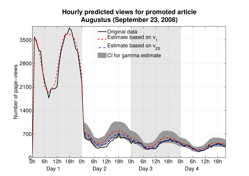
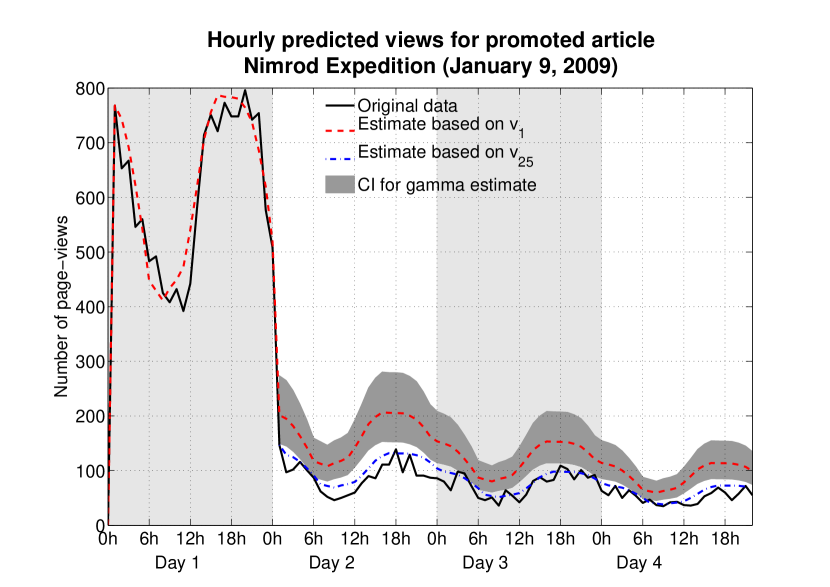
Figure 7: Examples of the prediction of the page-views for a promoted article.

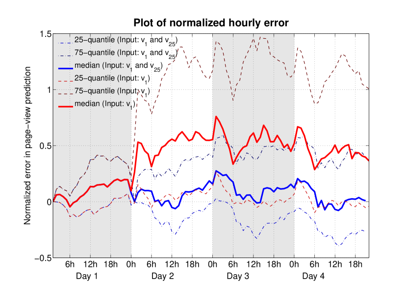
Figure 8: Hourly normalised errors.

We analyse the normalised hourly errors $(\hat{v}_{t}-v_{t})/v_{t}$ for all articles under study for both prediction methods: errors for just $v_{1}$ are plotted in red, while errors using both $v_{1}$ and $v_{25}$ in blue. From Figure 8 we observe that our prediction performs well for the first day of exposure. We recall that for this time interval we only use $v_{1}$ for the prediction. For the second, the third and the fourth days we observe an increase of the spread of hourly errors. However, this increase is not present for the second prediction technique.

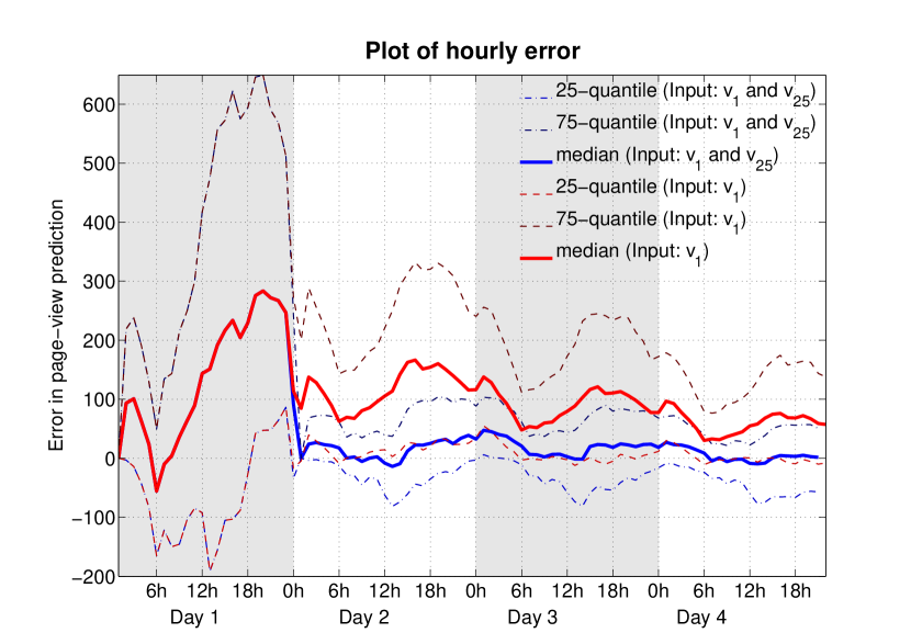
Figure 9: Hourly errors of actual page-views.

Finally, we present the absolute hourly errors $(\hat{v}_{t}-v_{t})$ in Figure 9. Interestingly, we observe that the absolute error towards the second half of day 1 is larger. This is caused by the fact that we model the negative jump only to occur during one specific hour whereas for some articles it actually starts a few hours before the end of the first day of the exposure duration. We also see that the hourly error during the second, the third and the fourth days are slightly increasing. This is similar to the observation in Figure 8. Again, the prediction method which uses both $v_{1}$ and $v_{25}$ as input outperforms the model that only uses $v_{1}$.

6 Conclusions and Discussion

We have presented a simple yet powerful model for the view dynamics of promoted content on Wikipedia. The model shows that the number of views an article receives decays exponentially in time with a constant decay rate if the dependency of the data on Wikipedia’s circadian activity cycle is removed. The only exception from this decay rule is the presence of a negative jump when an article is moved from the “today’s featured” to the list of “Recently featured” after 24h of being promoted, only to decrease later again with the same constant decay rate. The model allows to predict the popularity of an article using only the number of views it receives during the first hour of exposure. The quality of the prediction can be improved if the model is updated right after an article is moved to the “Recently featured” section.

Our model, based on the Poisson process, provides a simpler mechanism to explain page-view behaviour than other recent studies (e.g. [15, 12]). It should allow to describe and compare view dynamics on other websites or parts of websites with similar update strategies, e.g. online newspapers which are updated on a daily basis, or a list of today’s recommended items (mobile apps, products, etc).

The decay factor can be a useful parameter to account for the half-live of a piece of content on a given site. The findings might also be useful to predict the success rate of new online advertisements or sponsored content in general.

References

- [1] F. Duarte, B. Mattos, A. Bestavros, V. Almeida, and J. Almeida. Traffic characteristics and communication patterns in blogosphere. In Proc. of ICWSM-06, 2006.
- [2] A. Kaltenbrunner, V. Gómez, and V. López. Description and prediction of slashdot activity. In Proceedings of LA-WEB 2007, 2007.
- [3] A. Kaltenbrunner and D. Laniado. There is no deadline - time evolution of Wikipedia discussions. In Proceedings of WikiSym’12. ACM, 2012.
- [4] R. Kumar, J. Novak, P. Raghavan, and A. Tomkins. On the bursty evolution of blogspace. World Wide Web, 8(2):159–178, 2005.
- [5] J. Lehmann, B. Gonçalves, J. J. Ramasco, and C. Cattuto. Dynamical classes of collective attention in Twitter. In Proceedings of WWW2012. ACM, 2012.
- [6] M. Mestyán, T. Yasseri, and J. Kertész. Early prediction of movie box office success based on Wikipedia activity big data. arXiv preprint arXiv:1211.0970, 2012.
- [7] F. Ortega. Wikipedia: A Quantiative Analysis. PhD thesis, Universidad Rey Juan Carlos, Madrid, Spain, 2009. http://libresoft.es/Members/jfelipe/phd-thesis.
- [8] M. Osborne, S. Petrovic, R. McCreadie, C. Macdonald, and I. Ounis. Bieber no more: First story detection using Twitter and Wikipedia. In Proceedings of TAIA’12, 2012.
- [9] J. Ratkiewicz, S. Fortunato, A. Flammini, F. Menczer, and A. Vespignani. Characterizing and modeling the dynamics of online popularity. Phys. Rev. Lett., 105:158701, 2010.
- [10] A. J. Reinoso, R. Muñoz-Mansilla, I. Herraiz, and F. Ortega. Characterization of the Wikipedia traffic. In Proceedings of ICIW 2012, 2012.
- [11] B. Suh, G. Convertino, E. Chi, and P. Pirolli. The singularity is not near: slowing growth of wikipedia. In Proceedings of WikiSym, 2009.
- [12] G. Szabo and B. A. Huberman. Predicting the popularity of online content. Commun. ACM, 53(8):80–88, Aug. 2010.
- [13] C. Wang, M. Ye, and B. A. Huberman. From user comments to on-line conversations. In Proceedings of SIGKDD, 2012.
- [14] S. West. Wikipedia’s evolving impact. TED2010, 2010. available at http://goo.gl/erGp2.
- [15] F. Wu and B. A. Huberman. Novelty and collective attention. PNAS, 104(45):17599–17601, 2007.
- [16] T. Yasseri, R. Sumi, and J. Kertész. Circadian patterns of Wikipedia editorial activity: A demographic analysis. PLoS ONE, 7(1):e30091, 2012.