Supersonic flow of a Bose-Einstein condensate past an oscillating attractive-repulsive obstacle

Abstract

We investigate by numerical simulations the pattern formation after an oscillating attractive-repulsive obstacle inserted into the flow of a Bose-Einstein condensate. For slow oscillations we observe a complex emission of vortex dipoles. For moderate oscillations organized lined up vortex dipoles are emitted. For high frequencies no dipoles are observed but only lined up dark fragments. The results shows that the drag force turns negative for sufficiently high frequency. We also successfully model the ship waves in front of the obstacle. In the limit of very fast oscillations all the excitations of the system tend to vanish.

I. INTRODUCTION

The realization of Bose-Einstein condensate (BEC) in atomic gases have boosted intense theoretical and experimental investigation about its exotic properties. BEC is a paradigm of a quantum fluid and in weak interacting case can well be described by the Gross-Pitaesvkii equation dalfovo . Eventually BEC spread to other systems like exciton-polaritons exciton2006 , offering new possibilities for experimental tests. An interesting feature of a quantum fluid is its contrasting behavior as compared with a classical fluid. The flow of a quantum fluid past an obstacle only generates drag force above a certain subsonic critical velocity and the energy can be dissipated into collective excitations of the fluid. This dissipation can be inferred from numerical experiments by the mean drag on the obstacle frisch . A superfluid behavior is revealed below this velocity where nucleation of vortices never occur and no excitations are generated jackson ; winiecki ; nore ; stiessberger ; huepe ; aftalion . For an appropriate velocity and size of the obstacle, a Bénard-von Kármám vortex street can be generated sasaki .

There is also a supersonic critical velocity where oblique vortex streets are transformed into stable oblique dark solitons kp-08 . For higher velocities, the general picture of the diffraction pattern in the supersonic flow past a disk-shaped impenetrable obstacle consists of two different parts separated by the Mach (or Cherenkov) cone egk-prl06 . Outside the Mach cone there is a region of linear waves that we will refer them simply as ship waves carusotto06 ; shipwaves . Inside the Mach cone a pair of oblique dark solitons is gradually formed behind the obstacle if the radius of the obstacle is of healing length order. For greater radius more pairs of oblique solitons are generated. Interaction of solitons was studied in annibale2011 ; khamis2012 where it was found that the angle between dark solitons decreases as the obstacle radius increases for a fixed supersonic velocity of the flow. In previous experimental works carusotto06 ; amo-2009 ; amo-2009-2 the existence of such nonlinear structures were suggested. However, only recently the generation of stable oblique dark solitons was experimentally demonstrated in the flow of a Bose-Einstein condensate of exciton-polaritons past an obstacle amo-2011 ; grosso2011 . A numerical study to support these experimental findings was done in pigeon , and the observation of vortex dipoles in an oblate atomic Bose-Einstein condensate brian suggests that the supersonic studies can also be carried in this system.

In atomic BEC, obstacles are typically represented by detuned lasers that can be effectively be attractive (red-detuned) or repulsive (blue-detuned) obstacles, by the use of Feshbach resonances. The first numerical study of attractive obstacles was done in Ref. jacksonattractive where it was established the critical velocity to the formation of vortices and corrects the velocity found in frisch in the case of repulsive obstacles. Numerical studies revealed that turbulence can also be achieved and studied by spatial oscillation of a repulsive obstacle tsubota . A clever way to control the formation of vortices moving attractive and repulsive laser beams was proposed in saito . There is a special form of moving potential that no radiation is generated at supersonic velocities law . The disappearance of gray soliton and phonon excitations was demonstrated in radouani by oscillating a repulsive obstacle in a quasi-1D trapped BEC at high obstacle velocities. It was found in saito2012 that vibration of an obstacle modulates the vortex street, theoretically predicted in sasaki , breaking a symmetry.

In the present work, we study the flow of a BEC past an oscillating attractive and repulsive obstacle. The motivation is to answer the question can we get rid of drag for very fast oscillations? We investigate different regimes from slow to very fast oscillations. Since we are working in the supersonic regime we can divide the study inside and outside the Mach cone as follows.

II. MODEL EQUATIONS

We consider the flow of an atomic Bose-Einstein condensate (BEC) past an obstacle in the framework of Gross-Pitaevskii (GP) mean field approach. In the rest frame, the condensate is well described by the macroscopic wave function $\Psi\equiv\Psi(x,y,z,t)$ obeying the time-dependent GP equation

$$i\hbar\frac{\partial\Psi}{\partial t}=-\frac{\hbar^{2}}{2m}\nabla^{2}\Psi+U_{ext}\,\Psi+\frac{4\pi a\hbar^{2}}{m}|\Psi|^{2}\Psi,$$ (1)

where $\nabla^{2}\equiv\partial^{2}_{x}+\partial^{2}_{y}+\partial^{2}_{z}$, the external potential $U_{ext}=U_{trap}(x,y,z)+U(x+vt,y,z,\Omega t)$ is represented by the sum of a harmonic trap $U_{trap}$ and a time-dependent obstacle potential $U$ that oscillates with frequency $\Omega$, $m$ is the atomic mass and $a$ is the s-wave scattering length.

We will limit our study to the case of the quasi-2D limit, i.e., we have a strong harmonic confinement in the $z$ direction. In this regime we can approximate $\Psi(x,y,z,t)=\psi(x,y,t)\phi(z)e^{-i\mu_{z}/\hbar}$, where $\phi(z)$ and $\mu_{z}$ are the ground state and energy respectively for the confinement in $z$ direction perez ; saito . Substituting in Eq.(1) and integrating in $z$ direction we obtain

$$i\hbar\frac{\partial\psi}{\partial t}=-\frac{\hbar^{2}}{2m}(\partial^{2}_{x}+\partial^{2}_{y})\psi+U\,\psi+g|\psi|^{2}\psi,$$ (2)

where $g=4\pi a\hbar^{2}m^{-1}\int\phi^{4}(z)dz$ is the effective interaction in two-dimensions. We consider here that the obstacle runs close to the center of the trap. In this region the condensate is almost homogeneous and the potential in $x$ and $y$ directions is weak as compared to the obstacle potential. So the harmonic potential is neglected for studying the excitation caused by the obstacle.

We introduce dimensionless variables ${\tilde{x}}=x/\xi$, ${\tilde{y}}=y/\xi$, ${\tilde{t}}=gn_{0}t/\hbar$, ${\tilde{\psi}}=\psi/\sqrt{n_{0}}$, ${\tilde{U}}=U/gn_{0}$, ${\tilde{\Omega}}=\Omega\hbar/gn_{0}$, the Mach velocity $M=v/c_{s}$, where $n_{0}$ is a characteristic 2D density of atoms at the center of the trap, $\xi=\hbar/\sqrt{mn_{0}g}$ is the characteristic length and the sound velocity $c_{s}=\hbar/m\xi$. Typical experimental values are $\xi\sim 0.3\mu$m and $\hbar/gn_{0}\sim 0.18$ms brian . Thus for ${\tilde{\Omega}\sim 1}$ we have oscillations of the order of kHz well within experimental reach. Substituting in Eq. (2) and after dropping the tildes for convenience we get

$$i\frac{\partial\psi}{\partial t}=-\frac{1}{2}(\partial^{2}_{x}+\partial^{2}_{y})\psi+U\psi+|\psi|^{2}\psi\,,$$ (3)

where $U=U(x+Mt,y,\Omega t)$. The energy is given by

$$E(t)=\int dxdy\left[{-\frac{1}{2}|\nabla_{x,y}\psi|^{2}+U|\psi|^{2}+\frac{1}{2}|\psi|^{4}}\right]\,,$$ (4)

and the rate of energy in time is given by

$$\frac{dE}{dt}=M\int dxdy|\psi|^{2}\frac{\partial U(\overline{x},y,\Omega t)}{\partial\overline{x}}|_{\overline{x}=x+Mt}+\int dxdy|\psi|^{2}\frac{\partial U(\overline{x},y,\Omega t)}{\partial t}|_{\overline{x}=x+Mt}\,.$$ (5)

Turning off the oscillation ($\Omega=0$) the second term vanishes and we identify the first term as $M$ times the drag force. Also when $M=0$ only the second term is responsible for the excitation of the system.

For computational purposes, in Eq. (3) we make a global phase transformation $\psi^{\prime}=e^{it}\psi$ and later a Galilean transformation $x^{\prime}=x+Mt$, $t^{\prime}=t$ leading to

$$i\frac{\partial\psi}{\partial t}=-\frac{1}{2}(\partial^{2}_{x}+\partial^{2}_{y})\psi-iM\partial_{x}\psi-\psi+|\psi|^{2}\psi+U\psi\,,$$ (6)

where $U=U(x,y,\Omega t)$, the primes were omitted for convenience and subscripts here means derivatives. This equation describes the system in the obstacle reference frame.

The obstacle is a laser beam that continuously oscillates from blue-detuned to red-detuned and vice-versa, which can be written as

$$U(x,y,\Omega t)=U_{0}\cos(\Omega t)\exp\left[\frac{-2\left(x^{2}+y^{2}\right)}{w_{0}^{2}}\right],$$ (7)

where $U_{0}$ and $w_{0}$ are the amplitude and the beam waist of the laser, respectively, and $\Omega=2\pi/T$ is the oscillation frequency of the detuning in a period $T$.

III. INSIDE THE MACH CONE

For $\Omega=0$ Eq. (6) supports stable oblique solitons egk-prl06 ; kp-08 ; khamis2012 in the obstacle frame as

$$\psi(x,y)=\frac{1+e^{\zeta+2i\alpha}}{1+e^{\zeta}}\,,$$ (8)

where $e^{i\alpha}\equiv\lambda+i\nu$, $\zeta\equiv 2\nu[x\sin\theta-y\cos\theta]$, $\nu\equiv\sqrt{1-\lambda^{2}}$, $\lambda\equiv M\sin\theta$, and $\theta$ is the angle between the soliton and the horizontal axis. $M\sin\theta=\pm 1$ defines the Mach cone and thus solitons can be found only in the region $-\arcsin(1/M)<\theta<\arcsin(1/M)$.

We have solved the Eq. (3) numerically in the supersonic regime using $U_{0}=25$ and $w_{0}=1$. In Fig. 1 we show the results for supersonic flow for different oscillation frequencies. Fig. 1 depicts the case of $\Omega=0$ where we reproduce the formation of oblique dark solitons egk-prl06 . Outside the Mach cone there is a stationary wave pattern created by interference of linear waves. Inside the Mach cone there are two oblique dark solitons that decay at the end points into vortices, situated symmetrically with respect to the direction of the flow. As we turn on the oscillations observe the emission of dark fragments. For $\Omega=0.5$ these fragments can be identified as vortex dipoles and form a pattern of “5 in a dice”. As the frequency is increased to $\Omega=1.5$ these fragments stand well aligned as vortex dipoles as can be identified by the phase plot (see Fig. 2). These dipoles are followed by a secondary radiation emission, identified as a straight line almost parallel to the Mach cone. As the frequency is further increased to $\Omega=10$ the fragments can no longer be identified neither as a single vortex nor as vortex dipoles. By looking at phase the fragments are identified as short gray solitons that propagate obliquely to the flow, analogous to the ones observed in Ref. flayac2012 . To check the (non)vorticity character after some time of fragments formation we turned off the intensity of the obstacle and no decay into vortices were observed.

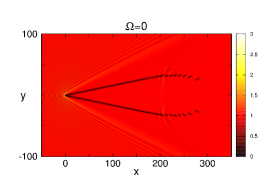
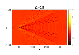
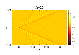
Figure 1: Pictures of the diffraction pattern at fixed time $t=100$ with the set of parameters: Mach number $M=3$, potential intensity $U_{0}=25$ (the laser beam starts repulsive) and width $w_{0}=1$ for different frequencies $\Omega=0$, 0.5, 1.5, 10 and 20.

One can explain the general behavior as following. For $\Omega=1.5$ the oscillation acts as a “chopper” that turns on and off the dipole emission. In this specific case the on time is more than enough to generate vortex dipoles and thus we have excess of energy that is ejected as secondary radiation. In the fast oscillating regime ($\Omega=10$) the time the oscillation is on is not enough to form dipoles and just small dark solitons can be seen. As the frequency is around $\Omega=20$ practically no more fragments can be seen. To check the consistency of our analysis we studied the number of fragments as a function of $\Omega$. One can estimate that rate of fragments emission is close to 1, meaning that at each period one fragment is emitted. The linear behavior confirms the modeling of the oscillating obstacle as a “chopper”.

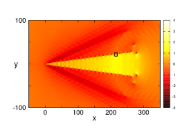
Figure 2: Left panel: Phase of the diffraction pattern that corresponds to Fig. 1 for frequency $\Omega=1.5$ which provides us evidence of vortex dipole formation. Right panel: inset showing vector velocities of the vortex dipole in the selected region. Note that the velocity in $x$ direction was not shifted by the constant flow velocity, $M$, for visualization purposes.

Thus we identified four regimes, for $\Omega\sim 0.5$ we have strange patterns as the “5 in a dice”, for $\Omega\sim 1.5$ we have lined vortex-dipoles with secondary radiation, for $\Omega\sim 10$ the dipoles are suppressed and give place to small dark solitons that propagate obliquely to the flow, finally for $\Omega\sim 20$ practically no excitation can be seen inside the Mach cone. If the laser beam starts red-detuned (attractive) we have similar results.

Next we develop the analytical theory to describe the remaining ship waves located outside the Mach cone and compare it with numerical simulations.

IV. OUTSIDE THE MACH CONE

Ship waves are formed in front of the obstacle. The theory for a non-oscillating obstacle was previously studied for a $\delta$ function in ref.khamis08 , where it was found that the density changes are given by

$$\delta n=V_{0}\,q(k,r,M)\times\cos\left(kr\cos\mu-\frac{\pi}{4}\right)$$ (9)

with

$$q(k,r,M)\equiv\sqrt{\frac{2k}{\pi r}}\frac{[(M^{2}-2)k^{2}+4(M^{2}-1)]^{1/4}}{[(M^{2}-2)k^{2}+6(M^{2}-1)]^{1/2}}\,,$$ (10)

and

$$k\equiv 2\sqrt{M^{2}\cos^{2}{\eta}-1}.$$ (11)

The angles $\mu$ and $\eta$ are defined according to Fig. 3, and Eq. (11) is valid if

$$-\arccos\left(\frac{1}{M}\right)\leq\eta\leq\arccos\left(\frac{1}{M}\right)~{},$$ (12)

so that the linear waves exist only in the region outside the Mach cone.

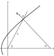
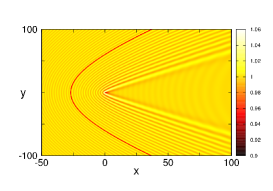
Figure 3: Left panel: Coordinates that defines the radius-vector ${\bf r}$ and the wave vector ${\bf k}$. The latter one is normal to the wave front which is shown schematically by a curved line. Right panel: Numerically calculated wave pattern for a fast oscillating obstacle at fixed time $t=100$ with the set of parameters: $M=2$, $U_{0}=25$, $w_{0}=1$ and $\Omega=40$. Solid line (red) corresponds to linear analytical theory (Eq. 13) for the line of constant phase.

According to khamis08 , one can find the shape of the lines of constant phase (wave crests) $\Phi=kr\cos\mu$ in a parametric form

$$\begin{split}&x=r\cos\chi=\frac{4\Phi}{k^{3}}\cos\eta(1-M^{2}\cos 2\eta),\\ &y=r\sin\chi=\frac{4\Phi}{k^{3}}\sin\eta(2M^{2}\cos^{2}\eta-1),\end{split}$$ (13)

so that for small values of $\eta$, corresponding to waves in front of the obstacle, these lines take a parabolic form

$$x(y)\cong-\frac{\Phi}{2\sqrt{M^{2}-1}}+\frac{(M^{2}-1)^{3/2}}{(2M^{2}-1)\Phi}y^{2}.$$ (14)

Predictions of the analytical theory are compared with the numerically calculated wave pattern in Fig. 3 and excellent agreement is found. So, the theory previously developed in khamis08 remains valid even for a fast oscillating obstacle.

For a fast oscillating we assume that the resulting ship waves can be computed by the Huygens principle, i.e., by the superposition of stationary densities generated by obstacles at different positions along the flow. Averaging over a period this can be expressed as

$$\delta n_{osc}=V_{0}\,q(k,r,M)\times\frac{1}{T}\int_{0}^{T}\cos(\Omega t)\cos\left(kr\cos\mu-\frac{\pi}{4}+kMt\right)~{}dt,$$ (15)

where the term $kMt$ was added representing phase change due to the obstacle movement along the time. After integration in time one obtains

$$\delta n_{osc}=\frac{1}{2\pi}V_{0}\,q(k,r,M)\left(\frac{-\Omega kM}{\Omega^{2}-k^{2}M^{2}}\right)\left[\sin\left(kr\cos\mu-\frac{\pi}{4}+kMT\right)-\sin\left(kr\cos\mu-\frac{\pi}{4}\right)\right].$$ (16)

In the region in front of the obstacle where $y=0$ (i.e. $\eta=0$) and $x<0$, the wavelength $\lambda=2\pi/k_{0}$ is constant with $k_{0}=2\sqrt{M^{2}-1}$. Therefore $x(0)=-r\cos\mu$ and the perturbations of the condensate density take the form

$$\delta n_{osc}=\frac{1}{2\pi}V_{0}\,q(k_{0},r,M)\left(\frac{-\Omega k_{0}M}{\Omega^{2}-k_{0}^{2}M^{2}}\right)\left[\sin\left(-k_{0}x-\frac{\pi}{4}+\frac{2\pi k_{0}M}{\Omega}\right)-\sin\left(-k_{0}x-\frac{\pi}{4}\right)\right],$$ (17)

where $r=|x|$. The above formulae shows that increasing $\Omega$ the magnitude of the $\delta n_{osc}$ decreases as $1/\Omega$ and in the limit of $\Omega\rightarrow\infty$ the ship waves vanish. The plot illustrating this behavior is shown in Fig. 4. As we see, Eq. (17) is accurate enough almost everywhere, for $\Omega\geq 40$, except in the small vicinity of the obstacle.

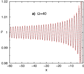
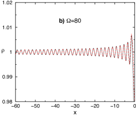
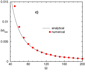
Figure 4: (a) and (b) Profile of intensity in front of the obstacle for $x<0$, $y=0$ with the set of parameters: $M=2$, $V_{0}=2$, $U_{0}=25$ (the laser beam starts repulsive) and $w_{0}=1$. Solid lines (black) correspond to linear analytical theory, Eq. (17), and dashed lines (red) to numerical solution of Eq. (3). (c) The solid line corresponds to the higher magnitude value of the $\delta n_{osc}$ close to $x=-40$ and the red circles correspond to this magnitude calculated numerically at the same position.

Although the obstacle in the theory is represented by a delta function, our numerical simulations using a narrow Gaussian potential as the obstacle provide results in very good agreement with our extended theory.

V. DRAG FORCE

We also computed the drag force in the $x$ direction as

$$F_{x}(t)=\int_{\mathcal{A}}\!dxdy\,|\psi|^{2}\,\frac{\partial U}{\partial x}\,,$$ (18)

where ${\mathcal{A}}$ defines an infinite region of the fluid around the obstacle. For practical purpose we took the integration along our whole grid. In Fig. 5 we show the average drag taken at one period of oscillation. For slow oscillation frequency $\Omega\lesssim 5$ we observe that drag is decreasing and positive as expected since both non-oscillating attractive and repulsive potentials causes positive drag jacksonattractive . However, for $\Omega\gtrsim 5$ the drag is always negative and vanishes in the limit of $\Omega\rightarrow\infty$. So, the answer for the question can we get rid of drag for very fast oscillations initially proposed is yes. Surprisingly, the mean drag also vanishes at a small region of low frequencies and this is a non-intuitive and remarkable result.

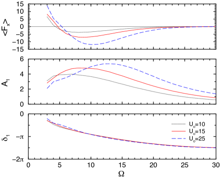
Figure 5: Upper panel: Average drag force in the $x$ direction, $<F_{x}>$, as a function of the frequency $\Omega$ for different potential intensities. Middle panel: response function amplitude $A_{1}$ as a function of $\Omega$. Lower panel: relative phase $\delta_{1}$ as a function of $\Omega$. Here we can see that the sign of $<F_{x}>$ depends on the relative phase between the forcing potential and the response main mode, Eq. (21).

The system can be seen as a forced oscillator. In our case the oscillating potential forces the system and we obtain as output an oscillating $|\psi|^{2}$. Thus the drag force in the $x$ direction can be explicitly written as

$$F_{x}=U_{0}\cos(\Omega t)R(t)\,,$$ (19)

where $R(t)$ is a response function given by

$$R(t)\equiv-\frac{4}{w_{0}^{2}}\int_{\mathcal{A}}x\exp\left[\frac{-2(x^{2}+y^{2})}{w_{0}^{2}}\right]|\psi(x,y,t)|^{2}dxdy\,.$$ (20)

We observed numerically that $R(t)$ is periodic with period $T$ and thus can be written as a Fourier series as

$$R(t)=A_{0}+A_{1}\cos(\Omega t+\delta_{1})+A_{2}\cos(2\Omega t+\delta_{2})+\cdots\,,$$ (21)

where $A^{\prime}s$ are amplitudes and $\delta^{\prime}s$ are relative phases to the forcing potential. Averaging the drag force in time we have

$$<F_{x}>=\frac{1}{T}\int_{0}^{T}U_{0}\cos(\Omega t)R(t)dt\,,$$ (22)

and only the second term of the series survives giving

$$<F_{x}>=\frac{U_{0}A_{1}}{\Omega}\cos(\delta_{1})\,.$$ (23)

Thus the sign of $<F_{x}>$ depends on the relative phase between the forcing potential and the response main mode. We computed

$$I\equiv\frac{1}{T}\int_{0}^{T}U_{0}\sin(\Omega t)R(t)dt=-\frac{U_{0}A_{1}}{\Omega}\sin(\delta_{1})\,$$ (24)

and from $<F_{x}>$ and $I$ we obtained $A_{1}$ and $\delta_{1}$.

A negative drag can be interpreted as a force in the upwind direction, meaning propels the laser. The question of the energy balance can be explained from the oscillating laser. As it attracts and repels the condensate it pumps energy to the system that causes an upwind force to supersede the downwind force due to the movement of the laser. This upwind force is only generated in the moving and oscillating obstacle. For standing $(M=0)$ oscillating obstacle the system is radially symmetric and no drag is generated.

VI. CONCLUSIONS

We have studied the wave pattern generated by an oscillating obstacle in the supersonic flow of a quantum fluid. Turning on oscillations causes disruption of the oblique solitons into dipoles. For $\Omega=1.5$ the dipoles are emitted organized as a vortex dipole street. For increasing frequencies dipoles change gradually orientation in clockwise direction and their bunch resembles the oblique solitons. Finally for very high frequencies the angle of emission increases and vortices vanishes. For the waves in front of the fast oscillating obstacle, we could further extend the model previously developed for non-oscillating obstacle. These waves were shown to gradually diminish according to the averaging of emission of linear waves out of phase. Combined results, both ship waves and soliton tend to vanish for high frequencies leading to a vanishing drag. Remarkably, the mean drag also vanishes at a small region of low frequencies during his change of sign from positive to negative. So, even a very powerful laser fast oscillating from red to blue-detuning could pass through an atomic BEC without generating vortices or solitons. This result could be experimentally checked with existing setups brian . Analogous experiments could also be performed with condensates of exciton-polaritons amo-2011 .

ACKNOWLEDGMENTS

EGK and AG thanks A.F.R.T. Piza, E.J.V. Passos, E.S. Annibale and F.Kh. Abdullaev for useful discussions. EGK thanks the support of G.A. El and the hospitality of the Department of Mathematical Sciences, Loughborough, where part of this work was carried out. We are also grateful to Conselho Nacional de Desenvolvimento Científico e Tecnológico and Fundação de Amparo à Pesquisa do Estado de São Paulo (Brazil) for financial support.

References

- (1) Dalfovo, Pitaesvkii, Stringari, Rev. Mod. Phys. (1999).
- (2) J. Kasprzak et al., Nature (London) 443, 409 (2006).
- (3) T. Frisch, Y. Pomeau, and S. Rica, Phys. Rev. Lett. 69, 1644 (1992).
- (4) B. Jackson, J. F. McCann, and C. S. Adams, Phys. Rev. Lett. 80, 3903 (1998).
- (5) T. Winiecki, J. F. McCann, and C. S. Adams, Phys. Rev. Lett. 82, 5186 (1999).
- (6) C. Nore, C. Huepe, and M. E. Brachet, Phys. Rev. Lett. 84, 2191 (2000).
- (7) J. S. Stießberger, and W. Zwerger, Phys. Rev. A 62, 061601(R) (2000).
- (8) C. Huepe, and M. E. Brachet, Physica D 140, 126 (2000).
- (9) A. Aftalion, Q. Du, and Y. Pomeau, Phys. Rev. Lett. 91, 090407 (2003).
- (10) K. Sasaki, N. Suzuki, and H. Saito, Phys. Rev. Lett. 104, 150404 (2010).
- (11) A. M. Kamchatnov and L. P. Pitaevskii, Phys. Rev. Lett. 100, 160402 (2008).
- (12) G.A. El, A. Gammal and A.M. Kamchatnov, Phys. Rev. Lett. 97, 180405 (2006).
- (13) I. Carusotto, S. X. Hu, L. A. Collins and A. Smerzi, Phys. Rev. Lett. 97, 260403 (2006).
- (14) Yu. G. Gladush, G. A. El, A. Gammal, A. M. Kamchatnov, Phys. Rev. A 75, 033619 (2007).
- (15) E. S. Annibale and A. Gammal, Phys. Lett. A 376, 46 (2011).
- (16) E. G. Khamis and A. Gammal, Phys. Lett. A 376, 2422 (2012).
- (17) A. Amo, J. Lefrère, S. Pigeon, C. Adrados, C. Ciuti, I. Carusotto, R. Houdré, E. Giacobino and A. Bramati, Nat. Phys. 5, 805 (2009).
- (18) A. Amo, D. Sanvitto, F. P. Laussy, D. Ballarini, E. del Valle, M. D. Martin, A. Lemaître, J. Bloch, D. N. Krizhanovskii, M. S. Skolnick, C. Tejedor and L. Viña, Nature 457, 291 (2009).
- (19) A. Amo, S. Pigeon, D. Sanvitto, V. G. Sala, R. Hivet, I. Carusotto, F. Pisanello, G. Lemenager, R. Houdre, E. Giacobino, C. Ciuti and A. Bramati, Science 332, 1167 (2011).
- (20) G. Grosso, G. Nardin, F. Morier-Genoud, Y. Léger, B. Deveaud-Plédran, Phys. Rev. Lett. 107, 245301 (2011).
- (21) S. Pigeon, I. Carusotto and C. Ciuti, Phys. Rev. B 83, 144513 (2011).
- (22) T. W. Neely, E. C. Samson, A. S. Bradley, M. J. Davis and B. P. Anderson, Phys. Rev. Lett. 104, 160401 (2010).
- (23) B. Jackson, J. F. McCann and C. S. Adams, Phys. Rev. A 61, 051603(R) (2000).
- (24) K. Fujimoto and M. Tsubota, Phys. Rev. A 83, 053609 (2011).
- (25) T. Aioi, T. Kadokura, T. Kishimoto and H. Saito, Phys. Rev. X 1, 021003 (2011).
- (26) C. K. Law, C. M. Chan, P. T. Leung, and M.-C. Chu, Phys. Rev. Lett. 85, 1598 (2000).
- (27) A. Radouani, Phys. Rev. A 70, 013602 (2004).
- (28) H. Saito, K. Tazaki, and T. Aioi, arXiv:1211.5869 (2012).
- (29) V. M. Pérez-García, H. Michinel, and H. Herrero, Phys. Rev. A 57 3837 (1998); K.K. Das, Phys. Rev. A 66, 053612 (2002).
- (30) H. Flayac, G. Pavlovic, M. A. Kaliteevski, and I. A. Shelykh, Phys Rev. B 85, 075312 (2012).
- (31) E.G. Khamis, A. Gammal, G. A. El, Yu. G. Gladush, and A. M. Kamchatnov, Phys. Rev. A 78, 013829 (2008).