Sampling Point Processes on Stable Unbounded Regions and Exact Simulation of Queues

Abstract

Given a marked renewal point process (assuming that the marks are i.i.d.) we say that an unbounded region is stable if it contains finitely many points of the point process with probability one. In this paper we provide algorithms that allow to sample these finitely many points efficiently. We explain how exact simulation of the steady-state measure valued state descriptor of the infinite server queue follows as a simple corollary of our algorithms. We provide numerical evidence supporting that our algorithms are not only theoretically sound but also practical. Finally, having simulation optimization in mind, we also apply our results to gradient estimation of steady-state performance measures.

1 Introduction

Let $N=\{N\left(t\right):t\in\left(-\infty,\infty\right)\}$ be a two sided time stationary renewal point process. We write $\{A_{n}:n\in\mathbb{Z}_{0}\}$ for the times at which the process $N$ jumps, where $\mathbb{Z}_{0}=\mathbb{Z}\backslash\{0\}$ denotes the set of integers removing zero, and with $A_{1}>0>A_{-1}$. For simplicity we assume that $A_{n}<A_{n+1}$ for every $n$. Further, we define $X_{n}=A_{n+1}-A_{n}$.

Now let $\{V_{n}:n\in\mathbb{Z}_{0}\}$ be a sequence of independent and identically distributed (i.i.d.) random variables (r.v.’s) which are independent of the process $N$. Define $Z_{n}=\left(A_{n},V_{n}\right)$ and consider the marked point process $\mathcal{M}=\{Z_{n}:n\in\mathbb{Z}_{0}\}$ which forms a subset of $\mathbb{R}^{2}$. We say that a (Borel measurable) set $\mathcal{B}$ is stable if $\left|\mathcal{M}\cap\mathcal{B}\right|<\infty$ almost surely (where $\left|\mathcal{C}\right|$ is used to denote the cardinality of the set $\mathcal{C}$).

Under natural assumptions on the inter-arrival times underlying $N$ and on the distribution of the $V_{n}$’s (stated in Section 2) we propose and study a class of algorithms that allow to sample exactly (i.e. without any bias) a realization of the set $\mathcal{M}\cap\mathcal{B}$ for a large class of unbounded, stable sets $\mathcal{B}$.

Our approach builds on algorithms that are fully developed and studied in [4]. As an application of the class of algorithms that we study here, we provide a procedure that allows to sample from the steady-state measure valued descriptor of an infinite server queue without any bias (i.e.exact simulation). Such a procedure, for instance, is obtained by considering the particular case in which $\mathcal{B}$ takes the form $\mathcal{B}=\{\left(t,v\right):v>\left|t\right|,t\leq 0\}$. Given that point processes constitute a natural way of constructing queueing models in great generality, we believe that the class of algorithms that we propose here have the potential to be applicable to the design of exact sampling algorithms of more general queueing models. This is a research avenue that we plan to investigate in the future.

We argue empirically that it is cheaper to run our exact sampling procedure to fully delete the initial bias than it is to do a burn-in period that reduces the bias to a reasonable size, say $5\%$, when talking about, for instance, the steady-state queue length.

Finally, we apply our exact sampling algorithms for infinite server queues to perform steady-state sensitivity analysis. For instance, we consider quantities such as the derivative of the steady-state average remaining service time with respect to the arrival rate or service rate. These quantities are of great interests in stochastic optimization via simulation.

So, in summary, our contributions are as follows:

i) We provide the first exact sampling algorithm for stationary marked renewal processes on unbounded and stable sets, see Section 2.

ii) As a corollary of i) we explain how to obtain an exact sampling algorithm for the steady-state measure valued descriptor of the infinite server queue. We also show empirically that this algorithm is practical in the sense of being both easy to code and fast to run, see Section 3.

iii) Finally, we provide new procedures for the sensitivity analysis of steady-state performance measures of the infinite server queue, see Section 4.

Relevant literature

Following the seminal work by [11], several exact sampling algorithms have been developed, particularly for spatial point processes. [9] and [10] developed algorithms and analytical tools based on so-called Dominated Coupling From the Past (DCFP). DCFP is based on the idea of introducing a stationary dominating process that is simulatable. Compared to our method, firstly they use spatial birth and death processes (generally of poisson type) as the coupled dominating processes. This would limit the target distribution to be absolutely continuous with respect to the Poisson measure. Secondly the number of steps simulated in the naive DCFP grows exponentially with the system scale (i.e. arrival rate in the infinite server queue setting); see Proposition 1 in [3] for a detailed proof. Although several modifications have been proposed, still the number of steps involved in these backward construction appears to be significantly large, especially when sampling in infinite volume regions [7]; see Section 7 in [3] for empirical comparisons.

Our method is based on a construction that is being used in [5] and [4]; see also [6] for related ideas. The method involves the technique of simulating the maximum of a negative drift random walk and the last passage time of independent and identically distributed random variables to an increasing boundary. As shown in [4] the complexity of our algorithm scales graciously as the system scale grows.

2 Sampling form stable unbounded regions

We start by discussing the assumptions behind our development.

Assumptions:

A1) Assume that $E\left|V_{n}\right|^{1/\alpha}<\infty$ for some $\alpha>0$, we also write $F\left(\cdot\right)=P\left(V_{n}\leq\cdot\right)$ for the cumulative distribution function (CDF) of $V_{n}$ and put $\overline{F}\left(\cdot\right)=1-F\left(\cdot\right)$ for the tail CDF.

A2) We assume that $F\left(\cdot\right)$ is known and easily accessible either in closed form or via efficient numerical procedures. Moreover, we can simulate $V_{n}$ conditional on $V_{n}\in[a,b]$ with $P\left(V_{n}\in[a,b]\right)>0$. Finally we can find $u(k)$ such that $u(k)\geq\int_{k}^{\infty}P(|V_{1}|^{1/\alpha}>\nu)d\nu$ and $u(k)\rightarrow 0$ as $k\rightarrow\infty$.

A3) Recall that $X_{n}=A_{n+1}-A_{n}>0$. Define $\psi\left(\theta\right)=\log E\exp\left(\theta X_{n}\right)$ and assume that there exists $\delta>0$ such that $\psi\left(\delta\right)<\infty$. Finally, let us write $\mu=EX_{n}$.

A4) Define $G\left(\cdot\right)=P\left(X_{n}\leq\cdot\right)$ and $\overline{G}\left(\cdot\right)=1-G\left(\cdot\right)$. Suppose that $G\left(\cdot\right)$ is known and that it is possible to simulate from $G_{eq}\left(\cdot\right):=\mu^{-1}\int_{\cdot}^{\infty}\overline{G}\left(t\right)dt$. Moreover, let $G_{\theta}\left(\cdot\right)=E\exp\left(\theta X_{n}-\psi\left(\theta\right)\right)I\left(X_{n}\leq\cdot\right)$ be the associated exponentially tilted distribution with parameter $\theta$ for $\psi\left(\theta\right)<\infty$. We assume that we can simulate from $G_{\theta}\left(\cdot\right)$.

Consider the class of sets $\mathcal{B}\subset\mathbb{R}^{2}$ that are Borel measurable and such that

$$\mathcal{B}\subset\mathcal{C}_{\alpha}=\{(t,v):\left|v\right|\geq|t|^{\alpha}\}.$$

Our goal in this section is to develop an algorithm that allows to sample without bias the random set $\mathcal{M}\cap\mathcal{C}_{\alpha}$, and therefore $\mathcal{M}\cap\mathcal{B}$. We will discuss extensions that follow immediately from our formulation at the end of this section. Figure 1 illustrates the different shapes that the set $\mathcal{C}_{\alpha}$ can take depending on the values of $\alpha>0$.

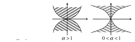
Figure 1: The area of $\mathcal{C}_{\alpha}$. The horizontal axis corresponds to the $t$ coordinate while the vertical axis represents the $v$ coordinate

We now proceed to explain our construction. As the stationary renewal point process is time reversible, starting at $0$ the distribution of the forward process $\{Z_{n}:n>0\}$ and the backward process $\{Z_{n}:n<0\}$ are the same. In what follows we limit our discussion to the construction of the forward process and the simulation of the backward process is completely analogous.

We follow the idea in [4]. Let $\epsilon\in(0,\mu)$. Consider any random time $\kappa$, finite with probability one but large enough such that

$A_{n+1}\geq n(\mu-\epsilon)$ and $\left|V_{n+1}\right|\leq(n(\mu-\epsilon))^{\alpha}$

for all $n\geq\kappa$.

If such random time $\kappa$ is well defined, we only need to simulate the stationary process up to $\kappa$ to get a sample from the unbounded region.

Proposition 1.

The random time $\kappa$ defined above exists and it is finite with probability one.

Proof.

By Chebyshev’s inequality,

$$P(A_{n+1}<n(\mu-\epsilon))\leq E[\exp(\theta(n(\mu-\epsilon)-A_{n+1})))\leq\exp(-n(-\theta(\mu-\epsilon)-\psi(-\theta)))$$

for any $\theta\geq 0$.
Let

$$I(-\epsilon)=\max_{\theta\geq 0}\{-\theta(\mu-\epsilon)-\psi(-\theta)\}$$

As $\psi(0)=0$, $\psi^{\prime}(0)=\mu$ and $\psi^{\prime\prime}(0)=Var(X)>0$, $I(-\epsilon)>0$. Then

$$P(A_{n+1}<n(\mu-\epsilon))\leq\exp(-nI(-\epsilon))$$

and

$$\sum_{n=1}^{\infty}P(A_{n+1}<n(\mu-\epsilon))\leq\frac{\exp(-I(-\epsilon))}{1-\exp(-I(-\epsilon))}<\infty$$

By Borel-Cantelli lemma, $\{A_{n+1}\geq n(\mu-\epsilon)\}$ eventually almost surely.
Similarly and independently we have

$$\sum_{n=1}^{\infty}P(\left|V_{n+1}\right|>(n(\mu-\epsilon))^{\alpha})=\sum_{n=1}^{\infty}P(\left|V_{1}\right|^{1/\alpha}>n(\mu-\epsilon))\leq\frac{1}{\mu-\epsilon}\int_{0}^{\infty}P(\left|V_{1}\right|^{1/\alpha}>\nu)d\nu<\infty$$

Thus, again by Borel-Cantelli lemma, $\{\left|V_{n+1}\right|\leq(n(\mu-\epsilon))^{\alpha}\}$ eventually almost surely. Therefore, $P(\kappa<\infty)=1$ ∎

As $\{A_{n}:n\geq 1\}$ and $\{V_{n}:n\geq 1\}$ are independent of each other, we consider the following construction. Let $\kappa(A)$ be a random time satisfying that $A_{n+1}\geq n(\mu-\epsilon)$ for $n\geq\kappa(A)$, and $\kappa(V)$ be a random time satisfying that $V_{n+1}\leq n(\mu-\epsilon)$ for $n\geq\kappa(V)$. Clearly $\kappa\left(A\right)$ and $\kappa\left(V\right)$ are not stopping times and this makes the simulation of these times challenging. However, we will explain how to sample these times and then we can set $\kappa=\max\{\kappa(A),\kappa(V)\}$. Our construction will allow us to simulate $\{A_{n}:n\geq 1\}$ and $\{V_{n}:n\geq 1\}$ separately.

2.1 Simulation of $\{A_{k}:1\leq k\leq\max\{n,\kappa\left(A\right)\}+1\}$

In this subsection we will introduce a method to simulate $\kappa(A)$ together with $\{A_{k}:k\geq 1\}$.

First, define $A_{1}$ according to the distribution $G_{eq}\left(\cdot\right)$. Sampling $A_{1}$ can be done according to A4).

Now, observe that $A_{n+1}=A_{1}+X_{1}+...+X_{n}$ and define

$$\tilde{S}_{n}=n(\mu-\epsilon)-\left(A_{n+1}-A_{1}\right)=\sum_{i=1}^{n}Y_{i},$$

where $Y_{i}=(\mu-\epsilon)-X_{i}$. Note that the $Y_{i}$’s are i.i.d. with $EY_{i}=-\epsilon$. If we set $\tilde{S}_{0}=0$, then $\{\tilde{S}_{n}:n\geq 0\}$ is a random walk with negative drift. We are interested in sampling up to the last time $n$ at which $\tilde{S}_{n}>0$.

We define the following sequence of random times:

$$\Delta_{1}=0,\text{ }\Gamma_{1}=\inf\{n\geq\Delta_{1}:\tilde{S}_{n}-\tilde{S}_{\Delta_{1}}>0\},$$

and for $j\geq 2$

$$\Delta_{j} =\inf\{n\geq\Gamma_{j-1}\mathbf{1}\{\Gamma_{j-1}<\infty\}\vee\Delta_{j-1}:\tilde{S}_{n}\leq 0\},$$

$$\Gamma_{j} =\inf\{n\geq\Delta_{j}:\tilde{S}_{n}-\tilde{S}_{\Delta_{j}}>0\}.$$

Now, let $\gamma=\inf\{j\geq 1:\Gamma_{j}=\infty\}$ and note that $\Delta_{\gamma+1}=\Delta_{\gamma}$ and that $\tilde{S}_{n}\leq 0$ for $n\geq\Delta_{\gamma}$, which in particular implies that $A_{n+1}\geq n(\mu-\epsilon)$ for $n\geq\Delta_{\gamma}$. Therefore, we have that $\Delta_{\gamma}=\kappa\left(A\right)$.

In what follows we will explain how to simulate the $\Delta_{j}$’s and $\Gamma_{j}$’s sequentially and jointly with the underlying random walk until time $\Delta_{\gamma}$. One important observation is that for every $j\geq 1$, $\Delta_{j}<\infty$ almost surely by the strong law of large numbers.

Let us write $\mathcal{F}_{n}=\sigma\{Y_{1},Y_{2},...,Y_{n}\}$ for the $\sigma$-field generated by the $Y_{j}$’s up to time $n$. Let $\xi\geq 0$ and define

$$T_{\xi}:=\inf\{n\geq 0:\tilde{S}_{n}>\xi\},$$

then by the strong Markov property we have that for $j\leq\gamma$,

$$P(\Gamma_{j}=\infty|\mathcal{F}_{\Delta_{j}})=P(\Gamma_{j}=\infty|\tilde{S}_{\Delta_{j}})=P(T_{0}=\infty)>0,$$

where we use $P\left(\cdot\right)$ to denote the nominal probability measure under which $\tilde{S}_{0}=0$.

It is important then to note that

$$P\left(\gamma=k\right)=P\left(T_{0}<\infty\right)^{k-1}P\left(T_{0}=\infty\right)$$

for $k\geq 1$. In other words, $\gamma$ is geometrically distributed. The procedure that we have in mind is to simulate $\Delta_{\gamma}$ in time intervals, and the number of time intervals is precisely $\gamma$.

Let $\psi_{Y}(\theta)=\log E\exp(\theta Y_{i})$. As the moment generating function of $X_{i}$ is finite in a neighborhood of the zero, $\psi_{Y}(\cdot)$ is also finite in a neighborhood of zero and $EY_{i}=\psi_{Y}^{\prime}(0)=-\epsilon$, Var$(Y_{i})=\psi_{Y}^{\prime\prime}(0)>0$. Then by the convexity of $\psi_{Y}(\cdot)$, one can always select $\epsilon>0$ sufficiently small so that there exists $\eta>0$ with $\psi_{Y}(\eta)=0$ and $\psi_{Y}^{\prime}(\eta)>0$. The root $\eta$ allows us to define a new measure $P_{\eta}$ based on exponential tilting so that

$$\frac{dP_{\eta}}{dP}\left(Y_{i}\right)=\exp(\eta Y_{i}).$$

Moreover, under $P_{\eta}$, $\tilde{S}_{n}$ is random walk with positive drift equal to $\psi_{Y}^{\prime}\left(\eta\right)$ ([1] P. 365). Therefore $P_{\eta}(T_{0}<\infty)=1$ and $P(T_{0}<\infty)=E_{\eta}(\exp(-\eta\tilde{S}_{T_{0}}))$. More generally, $P_{\eta}(T_{\xi}<\infty)=1$ and

$$q\left(\xi\right):=P(T_{\xi}<\infty)=E_{\eta}(\exp(-\eta\tilde{S}_{T_{\xi}}))$$

for each $\xi\geq 0$. Based on the above analysis we now introduce a convenient representation to simulate a Bernoulli random variable $J\left(\xi\right)$ with parameter $q\left(\xi\right)$ namely,

$$J\left(\xi\right)=I(U\leq\exp(-\eta\tilde{S}_{T_{\xi}})).$$ (1)

where $U$ is a uniform random variable independent of everything else under $P_{\eta}$.

Identity (1) provides the basis for an implementable algorithm to simulate a Bernoulli with success probability $q(\xi)$. Sampling $\{\tilde{S}_{1},...,\tilde{S}_{T_{0}}\}$ conditional on $T_{0}<\infty$, as we shall explain now, corresponds to basically the same procedure. First, let us write $P^{\ast}(\cdot)=P(\cdot|T_{0}<\infty)$. The following result provides an expression for the likelihood ratio between $P^{\ast}$ and $P_{\eta}$.

Lemma 1.

We have that

$$\frac{dP^{\ast}}{dP_{\eta}}(\tilde{S}_{1},...,\tilde{S}_{T_{0}})=\frac{\exp(-\eta\tilde{S}_{T_{0}})}{P(T_{0}<\infty)}\leq\frac{1}{P(T_{0}<\infty)}.$$

Proof.

$$P(\tilde{S}_{1}\in H_{1},...,\tilde{S}_{T_{0}}\in H_{T_{0}}|T_{0}<\infty) = \frac{P(\tilde{S}_{1}\in H_{1},...,\tilde{S}_{T_{0}}\in H_{T_{0}},T_{0}<\infty)}{P(T_{0}<\infty)}$$

$$= \frac{E_{\eta}[\exp(-\eta\tilde{S}_{T_{0}})I(\tilde{S}_{0}\in H_{0},...,\tilde{S}_{T_{0}}\in H_{T_{0}})]}{P(T_{0}<\infty)}.$$

∎

The previous lemma provides the basis for a simple acceptance / rejection procedure to simulate $\{\tilde{S}_{1},...,\tilde{S}_{T_{0}}\}$ conditional on $T_{0}<\infty$. More precisely, we propose $(\tilde{S}_{1},...,\tilde{S}_{T_{0}})$ from $P_{\eta}\left(\cdot\right)$. Then one generates a uniform random variable $U$ independent of everything else and accept the proposal if

$$U\leq\frac{1}{1/P(T_{0}<\infty)}\times\frac{dP^{\ast}}{dP_{\eta}}(\tilde{S}_{1},...,\tilde{S}_{T_{0}})=\exp(-\eta\tilde{S}_{T_{0}}).$$

This criterion coincides with $J\left(0\right)$ according to (1). So, the procedure above simultaneously obtains both a Bernoulli r.v. $J\left(0\right)$ with parameter $q\left(0\right)$, and the corresponding path $\{\tilde{S}_{1},...,\tilde{S}_{T_{0}}\}$ conditional on $T_{0}<\infty$.

Algorithm 1 (Outputs $(\tilde{S}_{0},...,\tilde{S}_{\Delta_{\gamma}})$)

• Set $K=0$, and $S_{0}=0$

• Simulate $(\tilde{S}_{1},...,\tilde{S}_{T_{0}})$ from $P_{\eta}$ and compute $J:=J\left(0\right)$ according to (1).

• If $J=1$, then let $S_{K+j}=\tilde{S}_{j}$ for $j=1,...,T_{0}$ and update $K\longleftarrow K+T_{0}$. Then, go back to Step 1.
  Otherwise, $J=0$ (i.e. $\Delta_{\gamma}=K$), stop and output $\left(S_{0},...,S_{K}\right)$

Remark: It has been proved in [4] that the expected number of times we need to repeat Step 1 does not change with the system scale (i.e. the arrival rate).

We noted earlier that $\Delta_{\gamma}=\kappa\left(A\right)$ and Algorithm 1 together with the initial procedure to sample $A_{1}$ allows us to simulate $\left(A_{j+1}:0\leq j\leq\kappa\left(A\right)\right)$, and we know that $A_{n+1}\geq n(\mu-\epsilon)$ for $n\geq\kappa\left(A\right)$. We need to simulate $A_{n+1}$ for $n\leq\kappa=\max\{\kappa\left(A\right),\kappa\left(V\right)\}$, and $\kappa\left(V\right)$ is independent of $\kappa\left(A\right)$. So, there might be cases for which we will have to sample $A_{n+1}$ for $n>\kappa\left(A\right)$. Since $A_{n+1}=A_{1}-\tilde{S}_{n}+n(\mu-\epsilon)$ it suffices to explain how to simulate $\tilde{S}_{n}$ for $n>\Delta_{\gamma}$. In turn, it suffices to explain how to simulate $(\tilde{S}_{n}:n\geq 0)$ with $\tilde{S}_{0}=0$ conditional on $T_{0}=\infty$. We will once again apply an acceptance / rejection procedure but this time we will use the original (nominal) distribution as the proposal distribution. Define

$$P^{\prime}\left(\cdot\right)=P(\cdot|T_{0}=\infty).$$

The following result provides an expression for the likelihood ratio between $P^{\prime}$ and $P$.

Lemma 2.

We have that

$$\frac{dP^{\prime}}{dP}(\tilde{S}_{1},...,\tilde{S}_{l})=\frac{I(T_{0}>l)(1-q(-\tilde{S}_{l}))}{P(T_{0}=\infty)}\leq\frac{1}{P(T_{0}=\infty)}.$$

Proof.

$$P(\tilde{S}_{1}\in H_{1},....,\tilde{S}_{l}\in H_{l}|T_{0}=\infty) = \frac{P(\tilde{S}_{1}\in H_{1},...\tilde{S}_{l}\in H_{l},T_{0}=\infty)}{P(T_{0}=\infty)}$$

$$= \frac{E[I(\tilde{S}_{1}\in H_{1},...,\tilde{S}_{l}\in H_{l})I(T_{0}>l)P(T_{0}=\infty|\tilde{S}_{0},...,\tilde{S}_{l})]}{P(T_{0}=\infty)}.$$

The result then follows from the strong Markov property and homogeneity of the random walk. ∎

We are in good shape now to apply acceptance / rejection to sample from $P^{\prime}$. The previous lemma indicates that to sample $\{\tilde{S}_{0},...,\tilde{S}_{l}\}$ given $T_{0}=\infty$ we can propose from the original (nominal) distribution and accept with probability $q(-\tilde{S}_{l})$ as long as $\tilde{S}_{j}\leq 0$ for all $0\leq j\leq l$. So, in order to perform the acceptance test we need to sample a Bernoulli with parameter $q(-\tilde{S}_{l})$, but this is easily done using identity (1). Thus we obtain the following procedure.

Algorithm 2 (Given $n\geq 0$ outputs $\{A_{1},A_{2},...,A_{\max\{n,\kappa(A)\}+1}\}$)

• Run Algorithm 1 and obtain $\{S_{0},S_{1},...,S_{K}\}$.

• If $K=\kappa\left(A\right)\geq n$, jump to Step 6. Otherwise, $K<n$, let $l=n-K\geq 1$.

• Simulate $\{\tilde{S}_{0},\tilde{S}_{1},...,\tilde{S}_{l}\}$ from the original (nominal) distribution with $\tilde{S}_{0}=0$.

• If $\tilde{S}_{j}\leq 0$ for all $0\leq j\leq l$ then sample a Bernoulli $J(-\tilde{S}_{l})$ with parameter $q(-\tilde{S}_{l})$ using (1) and continue to Step 5. Otherwise (i.e. $\tilde{S}_{j}>0$ for some $1\leq j\leq l$) go back to Step 3.

• If $J(-\tilde{S}_{l})=1$, go back to Step 3. Otherwise, $J(-\tilde{S}_{l})=0$, let $S_{K+i}=S_{K}+\tilde{S}_{i}$ for $i=1,2,...,l$

• Let $m=\max\{n,\kappa(A)\}$. Simulate $A_{1}$ with CDF $G_{eq}(\cdot)=\mu^{-1}\int_{\cdot}^{\infty}\bar{G}(t)dt$. Set $A_{n+1}=A_{1}-S_{n}+n(\mu-\epsilon)$ for $n=1,...,m$. Output $\{A_{1},...,A_{m+1}\}$.

2.2 Simulation of $\{V_{n}:1\leq n\leq\kappa(V)+1\}$

In this section we will introduce a method to simulate $\kappa(V)$ together with the $\{V_{n}:n\geq 1\}$.

Let $p(n)=P(|V_{1}|>(n(\mu-\epsilon))^{\alpha})$. We define $\Upsilon_{0}=0$ and $\Upsilon_{i}=\inf\{n>\Upsilon_{i-1}:|V_{n+1}|>(n(\mu-\epsilon))^{\alpha}\}$ for $i=1,2,...$. We also define two independent sequences of random variables, $\{\hat{V}_{n+1}:n\geq 1\}$, and $\{\bar{V}_{n+1}:n\geq 1\}$ as follows. The elements in each sequence are i.i.d., $\hat{V}_{n+1}$ is distributed as $V_{n+1}$ conditional on $|V_{n+1}|>(n(\mu-\epsilon))^{\alpha}$, and $\bar{V}_{n+1}$ follows the distribution of $V_{n+1}$ conditional on $|V_{n+1}|\leq(n(\mu-\epsilon))^{\alpha}$. We simulate $V_{1}$ following its nominal distribution independent of everything else.

Let $\sigma=\inf\{i\geq 0:\Upsilon_{i}=\infty\}$. Then $V_{n+1}\leq(n(\mu-\epsilon))^{\alpha}$ for $n\geq\Upsilon_{\sigma-1}+1$. We next introduce a method to sample $\Upsilon_{1},\Upsilon_{2},...$ sequentially and jointly with the $V_{n}$’s up until $\Upsilon_{\sigma-1}$.

The following lemma provides the basis to guarantee the termination of our procedure.

Lemma 3.

If $E|V_{1}|^{1/\alpha}<\infty$, then

$$P(\Upsilon_{1}=\infty)=\prod_{i=1}^{\infty}(1-p(i))\geq\exp(-2E|V_{1}|^{1/\alpha}/(\mu-\epsilon))>0,$$

consequently $E\sigma\leq\exp(2E|V|^{1/\alpha}/(\mu-\epsilon))<\infty$.

Remark: The bound on $E\sigma$ can be improved. This improvement is important for the theoretical asymptotic analysis of GI/GI/$\infty$ application, see [4].

Proof.

$$P(\Upsilon_{1}=\infty)=\prod_{n=1}^{\infty}(1-p(n)) \geq \prod_{n=1}^{\infty}\exp(-2p(n))$$

$$\geq \exp(-\frac{2}{\mu-\epsilon}\int_{0}^{\infty}P(|V_{1}|^{1/\alpha}>\nu)d\nu)=\exp(-\frac{2E|V_{1}|^{1/\alpha}}{\mu-\epsilon})$$

For $i=2,3,...$ conditional on $\Upsilon(i-1)=k$:

$$P(\Upsilon_{i}=\infty|\Upsilon_{i-1}=k)=\prod_{n=k+1}^{\infty}(1-p(n))\geq\exp(-\frac{2\int_{k}^{\infty}P(|V_{1}|^{1/\alpha}>\nu)d\nu}{\mu-\epsilon}\geq\exp(-\frac{2E|V_{1}|^{1/\alpha}}{\mu-\epsilon})$$

Thus $\sigma$ is stochastically dominated by a geometric random variable with parameter $p=\exp(-2E|V_{1}|^{1/\alpha}/(\mu-\epsilon))$, the result then follows.

∎

Notice that

$$\prod_{i=k+1}^{l}(1-p(i))\geq P(\Upsilon_{i}=\infty|\Upsilon_{i-1}=k)\geq\prod_{i=k+1}^{l}(1-p(i))\times\exp(-\frac{2\int_{l}^{\infty}P(|V_{1}|^{1/\alpha}>\nu)d\nu}{\mu-\epsilon})$$ (2)

for $l\geq k+1$.
Thus if we are simulating $I\sim$ Bernoulli$(r_{i})$ with $r_{i}:=P(\Upsilon_{i}=\infty|\Upsilon_{i-1})$, then with probability one we can check whether $U\leq P(\Upsilon_{i}=\infty|\Upsilon_{i-1})$ for $U\sim$ Unif$[0,1]$ by making $l$ sufficiently large without calculating the infinite product in the definition of $P(\Upsilon_{i}=\infty|\Upsilon_{i-1})$.

On the other hand, if we define $\prod_{j=1}^{0}(1-p(j)):=1$, then

$$P(\Upsilon_{1}=n|\Upsilon_{1}<\infty)=p(n)\frac{\prod_{j=1}^{n-1}(1-p(j))}{P(\Upsilon_{1}<\infty)}\leq p(n)\frac{1}{P(\Upsilon_{1}<\infty)}.$$

Consider a random variable $N$ with the following probability density function

$$P(N=n)=cp(n)$$

for $n=1,2,...$, where $c=(\sum_{n=1}^{\infty}p(n))^{-1}$. Then $P(\Upsilon_{1}=n|\Upsilon_{1}<\infty)/P(N=n)\leq 1/(cP(\Upsilon_{1}<\infty)).$

So we can simulate $\Upsilon_{1}$ given $\Upsilon_{1}<\infty$ using acceptance / rejection with $N$ as the proposal random variable. Generalizing the idea to $\Upsilon_{i}$, we can obtain the following algorithm

Algorithm 3 (Given $\Upsilon_{i-1}=k$, outputs $\Upsilon_{i}$ conditional on $\Upsilon_{i}<\infty$)

• Let $c=(\sum_{n=k+1}^{\infty}p(n))^{-1}$. Simulate $N$ with probability density function $P(N=n)=cp(n)$ for $n=k+1,k+2,...$

• Simulate $U\sim$ Unif$[0,1]$ independently. If $U\leq\prod_{j=k+1}^{N-1}(1-p(j))$ , set $\Upsilon_{i}=N$ and stop. Otherwise go back to Step 1

We conclude this section with our procedure to simulate $\{V_{1},V_{2},...V_{\kappa(V)+1}\}$.

Algorithm 4 (Outputs $\{V_{1},V_{2},...V_{\kappa(V)+1}\}$)

• Set $\Upsilon_{0}=0$, $i=1$. Simulate $V_{1}$ from its nominal distribution.

• Simulate $I\sim$ Bernoulli$(r_{i})$ with $r_{i}:=P(\Upsilon_{i}=\infty|\Upsilon_{i-1})$ (see (2)).

• If $I=1$, set $\kappa(V)=\Upsilon_{i-1}+1$. Simulate $V_{\kappa(V)+1}$ by sampling from $\bar{V}_{\kappa(V)+1}$ and stop. Otherwise $I=0$, sample $\Upsilon_{i}$ conditional on $\Upsilon_{i}<\infty$ and the value of $\Upsilon_{i-1}$ using Algorithm 3. Simulate the process between $\Upsilon_{i-1}+2$ and $\Upsilon_{i}+1$ by sampling from $\bar{V}_{n}$ for $\Upsilon_{i-1}+2\leq n\leq\Upsilon_{i}$ and $\hat{V}_{n}$ for $n=\Upsilon_{i}+1$. Set $i=i+1$ and then go back to Step 1.

3 Application to the infinite server queue

As a direct application of the ideas discussed in the previous section we study steady-state simulation for the infinite server queue. The following diagram indicates how to construct the steady-state measure valued descriptor assuming that we can sample all the points inside the set

$$\mathcal{C}=\{(t,v):v\geq\left|t\right|,t\leq 0\}.$$

Let $Q(t,y)$ denote the number of people in the system at time $t$ with residual service time strictly greater than $y$ and $E(t)$ denote the time elapsed since the previous arrival at time $t$ (i.e. $E\left(\cdot\right)$ is the age process associated with $N\left(\cdot\right)$). Figure 2 below depicts the region $\mathcal{C}$. Every point in $\left|\mathcal{M}\cap\mathcal{C}\right|$ is projected to the vertical line at time zero by drawing a $-$45⁰ line. The final position in the vertical line if positive, represents the corresponding remaining service time. Since the underlying point process is time stationary, the whole configuration of points obtained by this procedure at time zero is a snap shot of the steady-state distribution of the infinite server queue.

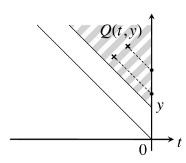
Figure 2: The points lies in the shaded area correspond to people who are still in the system at time $0$ with remaining service time greater than $y$

3.1 Algorithm for the Infinite Server Queue

As depicted in Figure 2 after projecting into the vertical line at $t=0$, we obtain the stationary remaining service requirements of the customers at time zero. We shall use $R_{1},R_{2},...,R_{Q(0,0)}$ to denote the remaining service times. The labeling is arbitrary although we will assign smaller indexes to customers that have spent less time in the system. Our algorithm proceeds as follows.

Algorithm 5 (Outputs $\{R_{1},R_{2},...,R_{Q(0,0)}\}$ and $E(0)$)

• Use Algorithm 4 to simulate the $\{V_{n},1\leq n\leq\kappa(V)+1\}$.

• Use Algorithm 2 to simulate the $\{A_{1},A_{2},...,A_{\max\{\kappa(V),\kappa(A)\}+1}\}$.

• Set $\kappa=\max(\kappa(V),\kappa(A))$. If $\kappa>\kappa(V)$, simulate $V_{n}$ by sampling from $\bar{V}_{n}$ for $n=\kappa(V)+2,...,\kappa+1$.

• Set $q=0$, $i=0$ and repeat the following procedure until $i=\kappa$:
  set $i=i+1$; if $V_{i}>A_{i}$, set $q=q+1$ and $R_{q}=V_{i}-A_{i}$.
  Output $\{R_{1},R_{2},...R_{q}\}$ and $A_{1}$.

3.2 Empirical Performance

Let $Y=\{Y(t):t\geq 0\}$ be a continuous time Markov process on the state space $\Omega$ and $f$ is a real-valued function defined on $\Omega$. The ergodic theorem guarantees in great generality (assuming a unique stationary distribution $\pi\left(\cdot\right)$) that

$$\frac{1}{t}\int_{0}^{t}f(Y(s))ds\rightarrow\int_{\Omega}f(y)\pi(dy)$$

as $t\rightarrow\infty$ almost surely for every positive, measurable function $f\left(\cdot\right)$. In the setting of the infinite server queue such a stationary distribution exists if $EV_{n}<\infty$ and $EX_{n}<\infty$. The most natural estimator for $E_{\pi}f(Y):=\int_{\Omega}f(y)\pi(dy)$ is therefore

$$\Phi(t,Y(0)):=\frac{1}{t}\int_{0}^{t}f(Y(s))ds,$$

where $Y(0)$ is the initial state. The estimator $\Phi\left(t,Y(0)\right)$ is generally biased unless $Y\left(0\right)$ is sampled from the stationary distribution $\pi\left(\cdot\right)$ ([2] P. 97). Our algorithm has the obvious advantage of removing the initial transient.

In what follows we conduct some simulation experiment to evaluate the practical performance of our algorithm. The idea is to fix a reasonable tolerance error, say 10%, for a given performance measure. Then we want to empirically find how large a burn-in period one would need in practice to reduce the initial transient bias to about 10%. In order to effectively quantify the error we select a class of systems for which $\pi\left(\cdot\right)$ can be explicitly evaluated.

We consider an infinite server queue with Poisson arrivals and Lognormal service times. As we are interested in the efficiency of our algorithm for relatively large systems, we set the arrival rate $\lambda=100$ and the service time $V_{n}\sim$ Lognormal$(-0.25,0.5)$ (i.e. $V_{n}$ has the same distribution as $\exp\left(-.25+.5\times N(0,1)\right)$, where $N\left(0,1\right)$ denotes a standard Gaussian random variable).

Let $Y(t)=(Q(t,\cdot),E(t))\in\mathcal{D}[0,\infty)\times\mathbb{R}_{+}$, then $Y(t)$ is a Markovian measure valued descriptor of the infinite server queue (of course in the Poisson arrival case one does not need to keep track of $A\left(\cdot\right)$).

We first compare the performance of our algorithm to the burn-in period defined as the period needed to reduce the initial transient as indicated earlier. Let $f(Y(t))=Q(t,0)$, i.e. the number of people in the system at time $t$. We measure the computation effort of the algorithm in terms of the number of arrivals (we call this the number of steps) simulated. Given $\epsilon>0$ we let $n(\epsilon)$ denote the minimum number of steps required so that $|E\Phi(A_{n(\epsilon)},(\phi,0))-E_{\pi}Q(0,0)|/E_{\pi}Q(0,0)\leq\epsilon$, where $(\phi,0)$ denotes a system that starts empty with $E(0)=0$ (recall that $E(\cdot)$ is the age process associated with $N(\cdot)$, i.e. when $E(0)=x$, $A_{1}$ is distributed as $X_{n}$ conditional on $X_{n}>x$). Table 1 shows the relation between $\epsilon$ and $n(\epsilon)$, obtained empirically based on the average of $10^{4}$ independent replications

Table 1: Bias of $\Phi(S_{n(\epsilon)})$

$\epsilon$	$n(\epsilon)$	computer time (s)
$10.26\%$	$6\times 10^{2}$	$0.0310$
$5.71\%$	$1\times 10^{3}$	$0.0382$
$1.17\%$	$5\times 10^{3}$	$0.1367$

Compared to the results in Table 1, our algorithm is unbiased. The average number of steps involved is $n=592.6369$ based on the average of $10^{4}$ independent replications and the average computer time needed for a single replication is $0.0249$ s.

In addition, in Table 2 we compare the performance of the estimators $\Phi(A_{n},(\phi,0))$ and $\Phi(A_{n^{\prime}},(Q(0,\cdot),A_{1}))$, where $Q(0,\cdot)$ and $A_{1}$ are sampled according to Algorithm 5. $n$ and $n^{\prime}$ are calibrated so that the computation budget is basically the same in both estimators. Under our procedure, $E\kappa$, the average number of arrivals required to terminate is approximately equal to $600$. So for instance, the first row in Table 2 corresponds to $n=10^{4}$. This means that $n^{\prime}\approx 9.4\times 10^{3}=10^{4}-600$. The true value of $E_{\pi}Q(0,0)$ is $88.2497$. The sample mean and sample standard deviation are calculated using the method of Batch means. The result in Table 2 shows that our mixed method performs better than the batch means with relatively small computation budget, while with large budget, the two methods are about the same.

Table 2: Simulation result with different initial states.

	$(\phi,0)$		$(Q(0,\cdot),A_{1})$
$n$	Sample Mean	Sample Std	Sample Mean	Sample Std
$1\times 10^{4}$	$86.1274$	$1.0104$	$88.1713$	$0.6018$
$5\times 10^{4}$	$89.0893$	$0.4587$	$88.2956$	$0.3770$
$1\times 10^{5}$	$88.5151$	$0.3531$	$88.1270$	$0.2976$
$5\times 10^{5}$	$88.3022$	$0.1481$	$88.3581$	$0.1402$

4 Application to sensitivity analysis of the infinite server queue

In this section, we apply our algorithm to sensitivity analysis of the infinite server queue. We consider a sequence of systems indexed by $(\lambda,\nu),$ $\lambda>0,$ $\nu>0$. Given $\left(\lambda,\nu\right)$, the interarrival times are multiplied by $1/\lambda$, obtaining $X_{n}/\lambda$ for all $n$, and the service times are multiplied by $1/\nu$, thus we have $V_{n}/\nu$ for all $n$. We assume that $EV_{n}<\infty$ and $EX_{n}<\infty$. We will use the notation $Q_{\lambda,\nu}\left(\cdot\right)$ to denote the infinite server queue descriptor for the $\left(\lambda,\nu\right)$-system. Our strategy rests on the application of Infinitesimal Perturbation Analysis (IPA), see for instance [8] P. 386. We assume here that the interarrival times have a continuous distribution.

We illustrate the methodology by computing the sensitivity of the steady-state average remaining service time, which we denote by $E_{\pi}\bar{R}(\lambda,\nu)$; namely,

$$E_{\pi}\bar{R}(\lambda,\nu)=E_{\pi}\frac{1}{Q_{\lambda,\nu}\left(0,0\right)}\int_{0}^{\infty}yQ_{\lambda,\nu}\left(0,dy\right).$$

We also consider

$$E_{\pi}R^{\infty}(\lambda,\nu)=E_{\pi}(\inf\{y\geq 0:Q_{\lambda,\nu}\left(0,y\right)=0\}),$$

in words, the steady-state maximum remaining service time. In order to apply IPA we need to define a few quantities.

First, let us define $\bar{\Xi}(\lambda,\nu)$ to be the average elapsed service time of the customers that are present at time zero (given the construction of the stationary process $\{Q_{\lambda,\nu}\left(t,\cdot\right):t\in\left(-\infty,\infty\right)\}$, see Figure 2). That is,

$$\bar{\Xi}(\lambda,\nu)=\frac{1}{Q_{\lambda,\nu}\left(0,0\right)}\sum_{n=-1}^{-\infty}\frac{\left|A_{n}\right|}{\lambda}I\left(\frac{\left|A_{n}\right|}{\lambda}<\frac{V_{n}}{\nu}\right)$$

Likewise, define $\bar{V}(\lambda,\nu)$ as the average of the total service requirement of the customers that are present at time zero, namely

$$\bar{V}(\lambda,\nu)=\frac{1}{Q_{\lambda,\nu}\left(0,0\right)}\sum_{n=-1}^{-\infty}\frac{V_{n}}{v}I\left(\frac{\left|A_{n}\right|}{\lambda}<\frac{V_{n}}{\nu}\right).$$

Next, we define $\Xi^{(\infty)}\left(\lambda,\nu\right)$ as the elapsed service time of the customer with the maximum remaining service time at time zero and $V^{(\infty)}(\lambda,\nu)$ as his total service time requirement. Specifically, if we let $m=\arg\max\{n:V_{n}/\nu-|A_{n}|/\lambda\}$ then

$$\Xi^{(\infty)}\left(\lambda,\nu\right)=\frac{|A_{m}|}{\lambda}\mbox{ and }V^{(\infty)}(\lambda,\nu)=\frac{V_{m}}{\nu}$$

We then obtain the following representation for the derivatives of $E_{\pi}\bar{R}(\lambda,\nu)$ and $E_{\pi}R^{\infty}(\lambda,\nu)$ with respect to $\lambda$ and $\nu$.

Lemma 4.

We have that
i)

$$\frac{\partial}{\partial\lambda}E_{\pi}\bar{R}(\lambda,\nu)=\frac{1}{\lambda}E_{\pi}\bar{\Xi}(\lambda,\nu)\mbox{ and }\frac{\partial}{\partial\nu}E_{\pi}\bar{R}(\lambda,\nu)=-\frac{1}{\nu}E_{\pi}\bar{V}(\lambda,\nu).$$

ii)

$$\frac{\partial}{\partial\lambda}E_{\pi}R^{\infty}(\lambda,\nu)=\frac{1}{\lambda}E_{\pi}\Xi^{(\infty)}(\lambda,\nu)\mbox{ and }\frac{\partial}{\partial\nu}E_{\pi}R^{\infty}(\lambda,\nu)=-\frac{1}{\nu}E_{\pi}V^{(\infty)}(\lambda,\nu)$$

Proof.

We only give a proof of part i) here as the proof of part ii) is entirely analogous.
Let $R_{n}$ denote the remaining service time of the $n$th customer at time zero and $V_{n}$ as his total service time requirement, then $R_{n}\leq V_{n}$. Thus if $EV_{n}<\infty$, we have

$$E_{\pi}\bar{R}(\lambda,\nu)<\infty$$

for any $\lambda>0$,$\nu>0$.
For a fixed sample path $\omega$ constructed backward in time, let $R_{n}(\lambda,\nu,\omega)$, $n<0$, denote the remaining service time of customer $n$ (counting backward in time) at time $0$ in system $(\lambda,\nu)$. Then $R_{n}(\lambda,\nu,\omega)=(V_{n}(\omega)/\nu-|A_{n}(\omega)|/\lambda)^{+}$ and

$$\lim_{h\rightarrow 0}\frac{R_{n}(\lambda+h,\nu,\omega)-R_{n}(\lambda,\nu,\omega)}{h}=\frac{|A_{n}(\omega)|}{\lambda^{2}}1\{\frac{V_{n}(\omega)}{\nu}\geq\frac{|A_{n}(\omega)|}{\lambda}\}$$

$$\lim_{h\rightarrow 0}\frac{R_{n}(\lambda,\nu+h,\omega)-R_{n}(\lambda,\nu,\omega)}{h}=-\frac{V_{n}(\omega)}{\nu^{2}}1\{\frac{V_{n}(\omega)}{\nu}\geq\frac{|A_{n}(\omega)|}{\lambda}\}$$

Thus the derivative $\frac{\partial}{\partial\lambda}\bar{R}(\lambda,\nu)$ and $\frac{\partial}{\partial\nu}\bar{R}(\lambda,\nu)$ exists.
Let $\Xi_{n}$ denote the elapsed service time of the $n$th customer at time zeros and define $\Xi_{n}=V_{n}$ if he is no longer in the system at time zero, then $\Xi_{n}\leq V_{n}$. Therefore $E_{\pi}\frac{\partial}{\partial\lambda}\bar{R}(\lambda,\nu)<\infty$ and $E_{\pi}\frac{\partial}{\partial\nu}\bar{R}(\lambda,\nu)<\infty$.
As $|(\bar{R}_{n}(\lambda+h,\nu)-\bar{R}_{n}(\lambda,\nu))/h|\leq\max_{\kappa_{\lambda+h,\nu}<n<0}V_{n}/\lambda^{2}$ and $|(\bar{R}_{n}(\lambda,\nu+h)-\bar{R}_{n}(\lambda,\nu))/h|\leq\max_{\kappa_{\lambda,\nu+h}<n<0}V_{n}/\nu^{2}$, by Lebesgue Dominated Convergence Theorem, we have

$$\frac{\partial}{\partial\lambda}E_{\pi}\bar{R}(\lambda,\nu)=E_{\pi}\frac{\partial}{\partial\lambda}\bar{R}(\lambda,\nu)\mbox{ and }\frac{\partial}{\partial\nu}E_{\pi}\bar{R}(\lambda,\nu)=E_{\pi}\frac{\partial}{\partial\nu}\bar{R}(\lambda,\nu)$$

As the interarrival times have a continuous distribution, $P(V_{n}/\nu=|A_{n}|/\lambda)=0$ for $n<0$.
Combining the change of limit and the sample path analysis we have

$$\frac{\partial}{\partial\lambda}E_{\pi}\bar{R}(\lambda,\nu)=\frac{1}{\lambda}E_{\pi}\bar{\Xi}(\lambda,\nu)\mbox{ and }\frac{\partial}{\partial\nu}E_{\pi}\bar{R}(\lambda,\nu)=-\frac{1}{\nu}E_{\pi}\bar{V}(\lambda,\nu)$$

∎

Table 3 shows the simulated results of an infinite server queue with base (i.e. $\lambda=1$) interarrival times distributed as Gamma$(2,2)$ and base (i.e. $\nu=1$) service times distributed as Lognormal$(-0.25,0.5)$.

Table 3: Simulation result from exact sampling.

$(\lambda,\nu)$	$\frac{\partial}{\partial\lambda}E_{\pi}\bar{R}(\lambda,\nu)$	$\frac{\partial}{\partial\nu}E_{\pi}\bar{R}(\lambda,\nu)$	$\frac{\partial}{\partial\lambda}E_{\pi}R^{\infty}(\lambda,\nu)$	$\frac{\partial}{\partial\nu}E_{\pi}R^{\infty}(\lambda,\nu)$
$(80,1)$	$7.0741\times 10^{-3}$	$-1.1320$	$6.1022\times 10^{-3}$	$-2.8389$
$(100,1)$	$5.6470\times 10^{-3}$	$-1.1316$	$4.9379\times 10^{-3}$	$-2.9495$
$(120,1)$	$4.7236\times 10^{-3}$	$-1.1337$	$4.2337\times 10^{-3}$	$-3.0684$

References

• [1] S. Asmussen. Applied Probability and Queues. Spinger, New York, 2 edition, 2003.
• [2] S. Asmussen and P. Glynn. Stochastic Simulation. Spinger, New York, 2007.
• [3] K. Berthelsen and J. Møller. A primer on perfect simulation for spatial point process. Bull Braz Math Soc, 33(3):351–367, 2002.
• [4] J. Blanchet and J. Dong. Exact sampling of loss systems. in preparation, 2012.
• [5] J. Blanchet and K. Sigman. On exact sampling of stochastic perpetuities. J. Appl. Probab., 48A:165–182, 2011.
• [6] K. Ensor and P. Glynn. Simulating the maximum of a random walk. Journal of Statistical Planning and Inference, 85:127–135, 2000.
• [7] R. Fernandez, P. Ferrari, and N. Garcia. Perfect simulation for interacting point processes, loss networks and ising models. Stoch. Process. Appl., 102(1):63–88, 2002.
• [8] P. Glasserman. Monte Carlo Methods in Financial Engineering. Spinger, New York, 2003.
• [9] W. Kendall. Perfect simulation for area-interaction point processes. In L. Accardi and C.C. Heyde, editors, Probability Towards 2000, pages 218–234. Spinger, New York, 1998.
• [10] W. Kendall and J. Møller. Perfect simulation using dominating processes on ordered spaces, with application to locally stable point pocesses. Adv. Appl. Prob., 32:844–865, 2000.
• [11] J. Propp and D. Wilson. Exact sampling with coupled Markov chains and applications to statistical mechanics. Random Structures and Algorithms, 9:223–252, 1996.