Convergence of a fourth order singular perturbation of the $n$-dimensional radially symmetric Monge-Ampère equation

Abstract

This paper concerns with the convergence analysis of a fourth order singular perturbation of the Dirichlet Monge-Ampère problem in the $n$-dimensional radial symmetric case. A detailed study of the fourth order problem is presented. In particular, various a priori estimates with explicit dependence on the perturbation parameter ${\varepsilon}$ are derived, and a crucial convexity property is also proved for the solution of the fourth order problem. Using these estimates and the convexity property, we prove that the solution of the perturbed problem converges uniformly and compactly to the unique convex viscosity solution of the Dirichlet Monge-Ampère problem. Rates of convergence in the $H^{k}$-norm for $k=0,1,2$ are established, and illustrating numerical experiment results are also presented in the paper.

1 Introduction

In this paper we consider the following fourth order singularly perturbed Monge-Ampère problem:

$$-\varepsilon\Delta^{2}u^{\varepsilon}+\det(D^{2}u^{\varepsilon}) =f\qquad \text{in}\ \Omega,$$ (1a)

$$u^{\varepsilon} =g\qquad \text{on }{\partial}{\Omega},$$ (1b)

$$\Delta u^{\varepsilon} =\varepsilon\qquad \text{on }{\partial}{\Omega},$$ (1c)

where ${\varepsilon}>0$, $\Omega\subset\mathbf{R}^{n}$ is a convex domain and $f>0$ in ${\Omega}$. The above problem is a special case of the following fourth order singular perturbation problem:

$$\varepsilon\Delta^{2}u^{\varepsilon}+F(D^{2}u,\nabla u^{\varepsilon},u^{\varepsilon},x) =0\qquad \text{in }{\Omega},$$ (2a)

$$u^{\varepsilon} =g\qquad \text{on }{\partial}{\Omega},$$ (2b)

$$\Delta u^{\varepsilon} =\varepsilon\quad \text{on}\ {\partial}{\Omega}$$ (2c)

with $F(D^{2}u^{\varepsilon},\nabla u^{\varepsilon},u^{\varepsilon},x)=f(x)-\det(D^{2}u^{\varepsilon})$. Here, $D^{2}u^{\varepsilon}(x)$ and $\nabla u^{\varepsilon}(x)$ denote respectively the Hessian matrix and the gradient of $u^{\varepsilon}$ at $x\in{\Omega}$.

Problem (1), respectively (2), was proposed by the authors in [12] as a stepstone to develop efficient numerical methods, particularly Galerkin-type methods, for approximating the viscosity solution of the Dirichlet Monge-Ampère problem (cf. [13, 14]):

$$\text{det}(D^{2}u) =f\qquad \text{in}\ {\Omega},$$ (3a)

$$u =g\qquad \text{on}\ {\partial}{\Omega},$$ (3b)

respectively, the general fully nonlinear second order PDE problem:

$$F(D^{2}u,\nabla u,u,x) =0\qquad \text{in }{\Omega},$$ (4a)

$$u =g\qquad \text{on }{\partial}{\Omega}.$$ (4b)

We remark that since the boundary condition (1c) (resp., (2c)) is artificially imposed to make the perturbed problem well-posed; other type boundary conditions can be used in the place of (1c) (resp., (2c)) (cf. [12]).

Fully nonlinear second order PDEs, which have experienced extensive analytical developments in the past thirty years (cf. [16, 6]), arise from many scientific and engineering fields including differential geometry, optimal control, mass transportation, geostrophic fluid, meteorology, and general relativity (cf. [7, 16, 15, 2, 26, 3, 11] and the references therein). Fully nonlinear PDEs play a critical role in the solutions of these application problems because they appear one way or another in the governing equations. By the middle eighties the classical solution theory for fully nonlinear second order PDEs was well established (cf. [16, Chapter 17]). The classical framework was soon followed by a comprehensive viscosity (weak) solution theory (cf. [9, 7] and the references therein) after the introduction of viscosity solutions by Crandall and Lions in [8] for fully nonlinear first order Hamilton-Jacobi equations.

In contrast with the success of PDE analysis, numerical solutions for general fully nonlinear second order PDEs was a relatively untouched area until very recently (cf. [11] and the references therein). The lack of progress is mainly due to the following two facts: (i) the notion of viscosity solutions is nonvariational; (ii) the conditional uniqueness (i.e., uniqueness only holds in a restrictive function class) of viscosity solutions is difficult to handle at the discrete level. The first difficulty prevents a direct construction of Galerkin-type methods and forces one to use indirect approaches as done in [17, 12, 14] for approximating viscosity solutions; this is main focus of this paper. The second difficulty prevents any straightforward construction of finite difference methods because such a method does not have a mechanism to enforce the conditional uniqueness and often fails to capture the sought-after viscosity solution (cf. [11] and the reference therein). To overcome the above difficulties, inspired by the vanishing viscosity method for the Hamilton-Jacobi equations, in [12] we proposed to approximate the fully nonlinear problem (3) (resp. (4)) by the fourth order quasilinear problem (1) (resp. (2)). We called this approximation procedure the vanishing moment method. If the vanishing moment method converges, then the solution of the former can be computed via the solution of the latter. This can be achieved by using many existing numerical methodologies including all Galerkin-type methods. So far, all of the numerical experiments and the analysis of [12, 13, 14, 23, 22] show that the vanishing moment method works effectively.

The primary goal of this paper is to provide a rigorous proof of the convergence of the vanishing moment method applied to the Monge-Ampére equation in the radially symmetric case in dimension $n\geq 2$. Specifically, we shall give a detailed analysis of problem (1) in the radially symmetric case and prove the convergence of the solution $u^{\varepsilon}$ of problem (1) to the unique convex viscosity solution $u$ of problem (3). We also derive the rates of convergence for $u-u^{\varepsilon}$ in various of norms. These results then put the vanishing moment method on a solid footing and provides a partial theoretical foundation for the numerical work in [12, 13, 14, 23].

The remainder of the paper is organized as follows. In Section 2, we give the radially symmetric descriptions of problems (3) and (1). Sections 3 and 4, which are the bulk of this paper, is devoted to studying the existence, uniqueness, regularity and convexity of the solution of the singularly perturbed problem (1). With these results in hand, we prove the uniform convergence of the solution $u^{\varepsilon}$ of problem (1) to the unique convex viscosity solution $u$ of problem (3) in Section 5. In addition, we derive rates of convergence for $u-u^{\varepsilon}$ in the $H^{k}$-norm for $k=0,1,2$ in Section 6. We present a few illustrating numerical computational results in Section 7 and end the paper with some concluding remarks in Section 8.

2 Descriptions of radially symmetric problems

Standard space notation is adopted in this paper, we refer the reader to [4, 16] for their exact definitions. Unless stated otherwise, ${\Omega}=B_{R}(0)\subset\mathbf{R}^{n}$ ($n\geq 2$) stands for the ball centered at the origin with radius $R$. We do not assume ${\Omega}$ is the unit ball because many of our results will depend on the size of the radius $R$. The unlabeled letter $C$ is used to denote a generic positive constant independent of ${\varepsilon}$ that may take on different values at different occurrences.

Suppose that $f=f(r),f\not\equiv 0$ and $g=g(r)$ in (3), that is, $f$ and $g$ are radial. Then the solution $u$ of (3) is expected to be radial, namely, $u(x)$ is a function of $r:=|x|=\sqrt{\sum_{j=1}^{n}x_{j}^{2}}$. We set $\hat{u}(r):=\hat{u}(|x|)=u(x)$, and for the reader’s convenience, we now compute ${\Delta}u,{\Delta}^{2}u$ and $\mbox{det}(D^{2}u)$ in terms of $\hat{u}$ (cf. [21, 25]). First, a direct calculation shows $\frac{{\partial}r}{{\partial}x_{j}}={x_{j}}/{r}$ and $\frac{{\partial}}{{\partial}x_{j}}\Bigl{(}r^{-1}\Bigr{)}=-{x_{j}}/{r^{3}}$. By the chain rule we have

$$\frac{{\partial}u(x)}{{\partial}x_{j}} =\hat{u}_{r}(r)\frac{{\partial}r}{{\partial}x_{j}}=\hat{u}_{r}(r)\frac{x_{j}}{r},\quad\frac{{\partial}^{2}u(x)}{{\partial}x_{j}{\partial}x_{i}}=\frac{1}{r}\Bigl{(}\frac{1}{r}\hat{u}_{r}(r)\Bigr{)}_{r}x_{i}x_{j}+\frac{\hat{u}_{r}(r)}{r}\delta_{ij}.$$

Here, the subscripts stand for the derivatives with respect to the subscript variables.

Noting that $D^{2}u(x)$ is a diagonal perturbation of a scaled rank-one matrix $xx^{T}$, and since the eigenvalues of $xx^{T}$ are $0$ (with multiplicity $n-1$) and $|x|^{2}=r^{2}$ (with multiplicity $1$ and corresponding eigenvector $x$), the eigenvalues of $D^{2}u(x)$ are $\lambda_{1}:=\frac{\hat{u}_{r}(r)}{r}+r\Bigl{(}\frac{1}{r}\hat{u}_{r}(r)\Bigr{)}_{r}=\hat{u}_{rr}(r)$ (with multiplicity $1$), and $\lambda_{2}:=\frac{\hat{u}_{r}(r)}{r}$ (with multiplicity $n-1$). Thus,

$${\Delta}u(x)=\lambda_{1}+(n-1)\lambda_{2}=\hat{u}_{rr}(r)+\frac{n-1}{r}\hat{u}_{r}(r)=\frac{1}{r^{n-1}}\bigl{(}r^{n-1}\hat{u}_{r}\big{)}_{r},$$

$${\Delta}^{2}u(x)={\Delta}({\Delta}u)={\Delta}\Bigl{(}\frac{1}{r^{n-1}}\bigl{(}r^{n-1}\hat{u}_{r}\big{)}_{r}\Bigr{)}=\frac{1}{r^{n-1}}\Bigl{(}r^{n-1}\Bigl{(}\frac{1}{r^{n-1}}\bigl{(}r^{n-1}\hat{u}_{r}\big{)}_{r}\Bigr{)}_{r}\Bigr{)}_{r},$$

$$\mbox{det}(D^{2}u(x))=\lambda_{1}(\lambda_{2})^{n-1}=\hat{u}_{rr}(r)\Bigl{[}\frac{\hat{u}_{r}(r)}{r}\Bigr{]}^{n-1}=\frac{1}{nr^{n-1}}\bigl{(}(\hat{u}_{r}\big{)}^{n})_{r}.$$

Abusing the notion by denoting $\hat{u}(r)$ by $u(r)$, problem (3) becomes seeking a function $u=u(r)$ such that

$$\frac{1}{nr^{n-1}}\bigl{(}(u_{r}\big{)}^{n})_{r} =f\qquad\mbox{in }(0,R),$$ (5a)

$$u(R) =g(R),$$ (5b)

$$u_{r}(0) =0.$$ (5c)

We remark that boundary condition (5c) is due to the symmetry of $u=u(r)$.

Lemma 2.1.

Suppose that $r^{n-1}f\in L^{1}((0,R))$ and $f\geq 0$ a.e. on $(0,R)$. Then there exists exactly one real solution if $n$ is odd and there are exactly two real solutions if $n$ is even, to the boundary value problem (5). Moreover, the solutions are given by the formula

$$u(r)=\left\{\begin{array}[]{ll}g(R)\pm\int_{r}^{R}\bigl{(}nL_{f}(s)\bigr{)}^{\frac{1}{n}}\,\,ds&\qquad\mbox{if $n$ is even},\\ \\ g(R)-\int_{r}^{R}\bigl{(}nL_{f}(s)\bigr{)}^{\frac{1}{n}}\,\,ds&\qquad\mbox{if $n$ is odd}\end{array}\right.$$ (6)

for $r\in(0,R)$. Here, the function $L_{f}(s)$ is defined by

$$L_{f}(s):=\int_{0}^{s}t^{n-1}f(t)\,dt.$$ (7)

Since the proof is elementary (cf. [21, 25]), we omit it. Clearly, when $n$ is even, the first solution (with the “$+$” sign) is concave, and the second solution (with the “$-$” sign) is convex because $u_{r}$ and $u_{rr}$ are simultaneously positive and negative respectively in the two cases. When $n$ is odd, the real solution is convex.

Remark 2.1.

The above theorem shows that $u$ is $C^{2}$ at a point $r_{0}\in(0,R)$ as long as $f$ is $C^{0}$ at $r_{0}$ and $L_{f}(r_{0})\neq 0$. Also, $u$ is smooth in $(0,R)$ if $f$ is smooth in $(0,R)$. We refer the reader to [21, 25] for the precise conditions on $f$ at $r=0$ to ensure the regularity of $u$ at $r=0$, extensions to the complex Monge-Ampère equation, and generalized Monge-Ampère equations in which $f=f(\nabla u,u,x)$.

Similarly, it is expected that $u^{\varepsilon}=u^{\varepsilon}(r)$ is also radial, and the vanishing moment approximation (2) then becomes

$$-\frac{{\varepsilon}}{r^{n-1}}\Bigl{(}r^{n-1}\Bigl{(}\frac{1}{r^{n-1}}\bigl{(}r^{n-1}u^{\varepsilon}_{r}\big{)}_{r}\Bigr{)}_{r}\Bigr{)}_{r}+\frac{1}{nr^{n-1}}\bigl{(}(u^{\varepsilon}_{r}\big{)}^{n})_{r} =f\qquad\mbox{in }(0,R),$$ (8a)

$$u^{\varepsilon}(R) =g(R),$$ (8b)

$$u^{\varepsilon}_{r}(0)=0,\quad|u^{\varepsilon}_{rr}(0)|<\infty,\quad|u^{\varepsilon}_{rrr}(r)|=o\bigl{(}\frac{1}{r^{n-1}}\bigr{)} \quad\mbox{as }r\to 0^{+},$$ (8c)

$$u^{\varepsilon}_{rr}(R)+\frac{n-1}{R}u^{\varepsilon}_{r}(R) ={\varepsilon}.$$ (8d)

In the next sections, we shall analyze problem (8) which includes proving the existence, uniqueness and regularity of the solution. After this is done, we then show that the solution $u^{\varepsilon}$ of (8) converges to the unique convex solution of (5).

Integrating over $(0,r)$ after multiplying (8a) by $r^{n-1}$, using boundary condition (8c) and $\lim_{r\to 0^{+}}r^{n-1}\Bigl{(}u^{\varepsilon}_{rrr}+\frac{n-1}{r}u^{\varepsilon}_{rr}-\frac{n-1}{r^{2}}u^{\varepsilon}_{r}\Bigr{)}=0,$ we get

$$-{\varepsilon}r^{n-1}\Bigl{(}\frac{1}{r^{n-1}}\bigl{(}r^{n-1}u^{\varepsilon}_{r}\big{)}_{r}\Bigr{)}_{r}+\frac{1}{n}(u^{\varepsilon}_{r})^{n}=L_{f}\qquad\mbox{in }(0,R).$$ (9)

Introduce the new function $w^{\varepsilon}(r):=r^{n-1}u^{\varepsilon}_{r}(r)$. A direct calculation shows that $w^{\varepsilon}$ satisfies

$$-{\varepsilon}r^{n-1}\Bigl{(}\frac{1}{r^{n-1}}w^{\varepsilon}_{r}\Bigr{)}_{r}+\frac{1}{nr^{n(n-1)}}(w^{\varepsilon})^{n}=L_{f}\qquad\mbox{in }(0,R).$$ (10a)

Converting the boundary conditions (8c)–(8d) to $$w^{\varepsilon}$$ we have

$$w^{\varepsilon}(0)=w^{\varepsilon}_{r}(0) =0,$$ (10b)

$$w^{\varepsilon}_{r}(R) ={\varepsilon}R^{n-1}.$$ (10c)

In addition, since $w^{\varepsilon}_{r}=r^{n-1}u^{\varepsilon}_{rr}+(n-1)r^{n-2}u^{\varepsilon}_{r},$ and $w^{\varepsilon}_{rr}=r^{n-1}u^{\varepsilon}_{rrr}+2(n-1)r^{n-2}u^{\varepsilon}_{rr}+(n-1)(n-2)r^{n-3}u^{\varepsilon}_{r},$ we have

$$\frac{{\partial}^{j}w^{\varepsilon}}{{\partial}r^{j}}(0)=o\Bigl{(}\frac{1}{r^{n-1-j}}\Bigr{)}\qquad\text{for }0\leq j\leq\min\{2,n-1\}.$$ (11)

In summary, we have derived from (8a) a reduced equation (10a), which is second order and easier to handle. After problem (10) is fully understood, we then come back to analyze problem (8).

3 Existence, uniqueness, and regularity of vanishing moment approximations

We now prove that problem (10) possesses a unique nonnegative classical solution. First, we state and prove the following uniqueness result.

Theorem 3.1.

Problem (10) has at most one nonnegative classical solution.

Proof.

Suppose that $w^{\varepsilon}_{1}$ and $w^{\varepsilon}_{2}$ are two nonnegative classical solutions to (10a)–(10c). Let

$$\phi^{\varepsilon}:=w^{\varepsilon}_{1}-w^{\varepsilon}_{2}\qquad\text{and}\qquad\overline{w}^{\varepsilon}:=\left\{\begin{array}[]{ll}\displaystyle\mathop{\sum_{\alpha+\beta=n-1}}_{\alpha,\beta\geq 0}(w_{1}^{\varepsilon})^{\alpha}(w_{2}^{\varepsilon})^{\beta}&\text{if }w^{\varepsilon}_{1}=w^{\varepsilon}_{2}\vskip 3.0pt plus 1.0pt minus 1.0pt\\ \dfrac{(w^{\varepsilon}_{1})^{n}-(w^{\varepsilon}_{2})^{n}}{w^{\varepsilon}_{1}-w^{\varepsilon}_{2}}&\text{otherwise}.\end{array}\right.$$

Subtracting the corresponding equations satisfied by $w^{\varepsilon}_{1}$ and $w^{\varepsilon}_{2}$ yields

$$-{\varepsilon}r^{n-1}\Bigl{(}\frac{1}{r^{n-1}}\phi^{\varepsilon}_{r}\Bigr{)}_{r}+\frac{1}{nr^{n(n-1)}}\overline{w}^{\varepsilon}\phi^{\varepsilon} =0\qquad\mbox{in }(0,R),$$ (12a)

$$\phi^{\varepsilon}(0)=\phi^{\varepsilon}_{r}(0) =0,$$ (12b)

$$\phi^{\varepsilon}_{r}(R) =0.$$ (12c)

Noting that $\overline{w}^{\varepsilon}\geq 0$ in $[0,R]$, we have by the weak maximum principle [10, Theorem 2, page 329] $\max_{[0,R]}|\phi^{\varepsilon}(r)|=\max\{|\phi^{\varepsilon}(0)|,|\phi^{\varepsilon}(R)|\}=\max\{0,|\phi^{\varepsilon}(R)|\}.$ If $\phi^{\varepsilon}(R)=0$, then $\phi^{\varepsilon}\equiv 0$. If $\phi^{\varepsilon}(R)\neq 0$, then $\phi^{\varepsilon}$ takes its maximum or minimum value at $r=R$. However, the strong maximum principle [24, Theorem 4, page 7] implies that $\phi^{\varepsilon}_{r}(R)\neq 0$, which contradicts with boundary condition $\phi^{\varepsilon}_{r}(R)=0$. Hence, $\phi^{\varepsilon}\equiv 0$ which implies $w^{\varepsilon}_{1}\equiv w^{\varepsilon}_{2}$. ∎

Next, we prove that the existence of nonnegative solutions to problem (10).

Theorem 3.2.

Suppose $r^{n-1}f\in L^{1}((0,R))$ and $f\geq 0$ a.e. in $(0,R)$. Then there is a nonnegative classical solution to problem (10).

Proof.

We divide the proof into three steps.

Step 1: Let $\psi^{0}\in C^{2}([0,R])$ be a nonnegative function that satisfies $\psi^{0}(0)=\psi^{0}_{r}(0)=0$ and $\psi^{0}_{r}(R)={\varepsilon}R^{n-1}$. For example, we may take $\psi^{0}(r)=\frac{{\varepsilon}}{n}r^{n}$. We then define a sequence of functions $\{\psi^{k}\}_{k\geq 0}$ recursively by solving for $k=0,1,2,\cdots$

$$-{\varepsilon}r^{n-1}\Bigl{(}\frac{1}{r^{n-1}}\psi^{k+1}_{r}\Bigr{)}_{r}+\frac{1}{nr^{n(n-1)}}(\psi^{k})^{n-1}\psi^{k+1} =L_{f}(r)\qquad\mbox{in }(0,R),$$ (13a)

$$\psi^{k+1}(0)=\psi^{k+1}_{r}(0) =0,$$ (13b)

$$\psi^{k+1}_{r}(R) ={\varepsilon}R^{n-1}.$$ (13c)

We first show by induction that for any such sequence satisfying (13), there holds $\psi^{k}\geq 0$ in $[0,R]$ for all $k\geq 0$. Note that $\psi^{0}\geq 0$ by construction. Suppose that $\psi^{k}\geq 0$ in $[0,R]$. Since $f\geq 0$ and $f\not\equiv 0$, we have

$$-{\varepsilon}r^{n-1}\Bigl{(}\frac{1}{r^{n-1}}\psi^{k+1}_{r}\Bigr{)}_{r}+\frac{1}{nr^{n(n-1)}}(\psi^{k})^{n-1}\psi^{k+1}>0\qquad\mbox{in }(0,R).$$

Hence, $\psi^{k+1}$ is a supersolution to the linear differential operator appearing in the left-hand side of (13a). By the weak maximum principle [10, Theorem 2, page 329], we have

$$\min_{[0,R]}\psi^{k+1}(r)\geq\min\{0,\psi^{k+1}(0),\psi^{k+1}(R)\}=\min\{0,\psi^{k+1}(R)\}.$$

Now suppose that $\psi^{k+1}(R)<0$. Then since $\psi^{k+1}_{r}(R)={\varepsilon}R^{n-1}>0$, the strong maximum principle [24, Theorem 4, page 7] implies that $\psi^{k+1}\equiv\mbox{const}$ in $[0,R]$, which leads to a contradiction as $\psi^{k+1}(0)=0$. Thus, we must have $\psi^{k+1}(R)\geq 0$, and therefore, $\psi^{k+1}\geq 0$ in $[0,R]$. By the induction argument, we conclude that $\psi^{k}\geq 0$ in $[0,R]$ for all $k\geq 0$.

It then follows from the standard theory for linear elliptic equations (cf. [10, 16]) that (13) has a unique classical solution $\psi^{k+1}$. Hence the $(k+1)$th iterate $\psi^{k+1}$ is well defined and therefore so is the sequence $\{\psi^{k}\}_{k\geq 0}$.

Step 2: Next, we shall derive some uniform (in $k$) estimates for the sequence $\{\psi^{k}\}_{k\geq 0}$. To this end, we first prove that $\psi^{k+1}(R)$ can be bounded from above uniformly in $k$. Multiplying (13a) by $\psi^{k+1}$ and integrating by parts yields

$$-{\varepsilon}\psi^{k+1}_{r}(r)\psi^{k+1}(r)\Bigl{|}_{r=0}^{r=R}+{\varepsilon}\int_{0}^{R}|\psi^{k+1}_{r}(r)|^{2}\,dr$$ (14)

$$+{\varepsilon}\int_{0}^{R}\frac{n-1}{r}\psi^{k+1}_{r}(r)\psi^{k+1}(r)\,dr+\int_{0}^{R}\frac{1}{nr^{n(n-1)}}(\psi^{k}(r))^{n-1}|\psi^{k+1}(r)|^{2}\,dr$$

$$\hskip 72.26999pt=\int_{0}^{R}\psi^{k+1}(r)L_{f}(r)\,dr.$$

It follows from boundary conditions (13b) and (13c) that

$$-{\varepsilon}\psi^{k+1}_{r}(r)\psi^{k+1}(r)\Bigl{|}_{r=0}^{r=R}=-{\varepsilon}^{2}R^{n-1}\,\psi^{k+1}(R).$$ (15)

Integrating by parts gives us

$$\int_{0}^{R}\frac{1}{r}\psi^{k+1}_{r}(r)\psi^{k+1}(r)\,dr =\frac{1}{2r}\bigl{(}\psi^{k+1}(r)\bigr{)}^{2}\Bigr{|}_{r=0}^{r=R}+\int_{0}^{R}\frac{1}{2r^{2}}\bigl{(}\psi^{k+1}(r)\bigr{)}^{2}\,dr$$ (16)

$$=\frac{1}{2R}\bigl{(}\psi^{k+1}(R)\bigr{)}^{2}+\int_{0}^{R}\frac{1}{2r^{2}}\bigl{(}\psi^{k+1}(r)\bigr{)}^{2}\,dr.$$

By Schwarz, Poincaré, and Young’s inequalities, we get

$$\int_{0}^{R}\psi^{k+1}(r)L_{f}(r)\,dr\leq\frac{{\varepsilon}}{2}\int_{0}^{R}|\psi^{k+1}_{r}(r)|^{2}\,dr+\frac{C_{1}^{2}}{2{\varepsilon}}\int_{0}^{R}\bigl{(}L_{f}(r)\bigr{)}^{2}\,dr$$ (17)

for some positive constant $C_{1}=C_{1}(R)$. Combining (3)–(17) we obtain

$$-2{\varepsilon}^{2}R^{n-1}\,\psi^{k+1}(R)+{\varepsilon}\int_{0}^{R}|\psi^{k+1}_{r}(r)|^{2}\,dr+\frac{{\varepsilon}(n-1)}{R}\bigl{(}\psi^{k+1}(R)\bigr{)}^{2}$$ (18)

$$+\int_{0}^{R}\frac{{\varepsilon}(n-1)}{r^{2}}\bigl{(}\psi^{k+1}(r)\bigr{)}^{2}\,dr+\int_{0}^{R}\frac{2}{nr^{n(n-1)}}(\psi^{k}(r))^{n-1}|\psi^{k+1}(r)|^{2}\,dr$$

$$\hskip 130.08621pt\leq\frac{C_{1}^{2}}{{\varepsilon}}\int_{0}^{R}\bigl{(}L_{f}(r)\bigr{)}^{2}\,dr.$$

Let $z:=\psi^{k+1}(R),\ b:=\frac{2{\varepsilon}R^{n}}{n-1},$ and $c:=\frac{C_{1}^{2}R^{2}}{{\varepsilon}^{2}(n-1)}\bigl{(}L_{f}(R)\bigr{)}^{2}.$ Then from (18) we have $z^{2}-bz-c\leq 0$, which in turn implies that

$$z_{1}\leq z\leq z_{2},\quad\mbox{where}\quad z_{1}=\frac{b-\sqrt{b^{2}+4c}}{2},\quad z_{2}=\frac{b+\sqrt{b^{2}+4c}}{2}.$$

Since $-z_{2}<z_{1}$, the above inequality then infers that $|z|\leq z_{2}$. Thus, there exists a positive constant $C_{2}=C_{2}(R,L_{f})$ such that $\bigl{|}\psi^{k+1}(R)\bigr{|}\leq z_{2}\leq\frac{C_{2}}{{\varepsilon}}.$ Substituting this bound into the first term on the left-hand side of (18) we also get

$${\varepsilon}\int_{0}^{R}|\psi^{k+1}_{r}(r)|^{2}\,dr +\int_{0}^{R}\frac{{\varepsilon}(n-1)}{r^{2}}\bigl{(}\psi^{k+1}(r)\bigr{)}^{2}\,dr$$ (19)

$$+\int_{0}^{R}\frac{2}{nr^{n(n-1)}}\bigl{(}\psi^{k}(r)\bigr{)}^{n-1}|\psi^{k+1}(r)|^{2}\,dr$$

$$\leq C_{3}:=\frac{C_{1}^{2}R}{{\varepsilon}}\bigl{(}L_{f}(R)\bigr{)}^{2}+2{\varepsilon}^{2}R^{n-1}C_{2}.$$

Now using the pointwise estimate for linear elliptic equations [16, Theorem 3.7] we have

$$\max_{[0,R]}|\psi^{k+1}(r)|\leq\Bigl{(}\frac{C_{2}}{{\varepsilon}}+\frac{L_{f}(R)}{{\varepsilon}}\Bigr{)}.$$ (20)

Next, we show that $\psi^{k+1}_{r}$ is also uniformly bounded (in $k$) in $[0,R]$. To this end, integrating (13a) over $(0,r)$ after multiplying it by $r^{n(n-1)}$, and integrating by parts twice in the first term yields

$$\psi^{k+1}_{r}(r) =-\frac{(n^{2}-1)[n(n-1)-1]}{r^{n(n-1)}}\int_{0}^{r}s^{n(n-1)-2}\psi^{k+1}(s)\,ds$$ (21)

$$\,+\frac{n^{2}-1}{r}\psi^{k+1}(r)+\frac{1}{{\varepsilon}nr^{n(n-1)}}\int_{0}^{r}\bigl{(}\psi^{k}(s)\bigr{)}^{n-1}\psi^{k+1}(s)\,ds$$

$$\quad\,-\frac{1}{{\varepsilon}r^{n(n-1)}}\int_{0}^{r}s^{n(n-1)}L_{f}(s)\,ds$$

for all $r\in(0,R)$. Using L’Hôpital’s rule it is easy to check that the limit as $r\to 0^{+}$ of each term on the right-hand side of (21) is zero. Hence, each term is bounded in a neighborhood of $r=0$. Moreover, on noting that $\psi^{k}\geq 0$, by Schwarz inequality we have

$$\int_{0}^{r}\bigl{(}\psi^{k}(s)\bigr{)}^{n-1}\psi^{k+1}(s)\,ds$$ (22)

$$\leq\Bigl{(}\int_{0}^{r}s^{n(n-1)}\bigl{(}\psi^{k}(s)\bigr{)}^{n-1}\,ds\Bigr{)}^{\frac{1}{2}}\Bigl{(}\int_{0}^{r}\frac{1}{s^{n(n-1)}}\bigl{(}\psi^{k}(s)\bigr{)}^{n-1}|\psi^{k+1}(s)|^{2}\,ds\Bigr{)}^{\frac{1}{2}}.$$

Now in view of (19)–(22) we conclude that there exists a positive constant $C_{4}=C_{4}(R,L_{f})$ such that

$$\max_{[0,R]}|\psi^{k+1}_{r}(r)|\leq\frac{C_{4}}{{\varepsilon}^{\frac{n+2}{2}}}.$$ (23)

By (13a) we get

$$\psi^{k+1}_{rr}(r)=\frac{1}{r}\psi^{k+1}_{r}(r) +\frac{1}{{\varepsilon}nr^{n(n-1)}}\bigl{(}\psi^{k}(r)\bigr{)}^{n-1}\psi^{k+1}(r)$$ (24)

$$-\frac{1}{{\varepsilon}}L_{f}(r)\qquad\forall r\in(0,R).$$

Again, using L’Hôpital’s rule and (11) it is easy to check that the limit as $r\to 0^{+}$ of each term on the right-hand side of (24) exists, and therefore, each term is bounded in a neighborhood of $r=0$. Hence, it follows from (20) and (23) that there exists a positive constant $C_{5}=C_{5}(R,L_{f})$ such that

$$\max_{[0,R]}|\psi^{k+1}_{rr}(r)|\leq\frac{C_{5}}{{\varepsilon}^{n+1}}.$$ (25)

To summarize, we have proved that $\|\psi^{k+1}\|_{C^{j}([0,R])}\leq C({\varepsilon},R,n,L_{f})$ for $j=0,1,2$ and the bounds are independent of $k$. Clearly, by a simple induction argument we conclude that these estimates hold for all $k\geq 0$.

Step 3: Since $\|\psi^{k}\|_{C^{2}([0,R])}$ is uniformly bounded in $k$, then both $\{\psi^{k}\}_{k\geq 0}$ and $\{\psi^{k}_{r}\}_{k\geq 0}$ are uniformly equicontinuous. It follows from Arzela-Ascoli compactness theorem (cf. [10, page 635]) that there is a subsequence of $\{\psi^{k}\}_{k\geq 0}$ (still denoted by the same notation) and $\psi\in C^{2}([0,R])$ such that

$$\psi^{k} \longrightarrow\psi\ \text{ and }\ \psi^{k}_{r}\longrightarrow\psi_{r} \quad\mbox{uniformly in every compact set $E\subset(0,R)$ as }k\to\infty.$$

Testing equation (13a) with an arbitrary function $\chi\in C^{1}_{0}((0,R))$ yields

$${\varepsilon}\int_{0}^{R}\psi^{k+1}_{r}(r)\chi_{r}(r)\,dr+{\varepsilon}\int_{0}^{R}\frac{n-1}{r}\psi^{k+1}_{r}(r)\chi(r)\,dr$$

$$\quad+\int_{0}^{R}\frac{1}{nr^{n(n-1)}}\bigl{(}\psi^{k}(r)\bigr{)}^{n-1}\psi^{k+1}(r)\chi(r)\,dr=\int_{0}^{R}L_{f}(r)\chi(r)\,dr.$$

Setting $k\to\infty$ and using the Lebesgue Dominated Convergence Theorem, we obtain

$${\varepsilon}\int_{0}^{R}\psi_{r}(r)\chi_{r}(r)\,dr +{\varepsilon}\int_{0}^{R}\frac{n-1}{r}\psi_{r}(r)\chi(r)\,dr$$ (26)

$$+\int_{0}^{R}\frac{1}{nr^{n(n-1)}}\bigl{(}\psi(r)\bigr{)}^{n}\chi(r)\,dr=\int_{0}^{R}L_{f}(r)\chi(r)\,dr.$$

Since $\psi\in C^{2}([0,R])$, we are able to integrate by parts in the first term on the left-hand side of (26), yielding

$$\int_{0}^{R}\Bigl{[}-{\varepsilon}\psi_{rr}(r)+\frac{{\varepsilon}(n-1)}{r}\psi_{r}(r)+\frac{1}{nr^{n(n-1)}}\bigl{(}\psi(r)\bigr{)}^{n}-L_{f}(r)\Bigr{]}\chi(r)\,dr=0$$

for all $\chi\in C^{1}_{0}((0,R))$. This then implies that

$$-{\varepsilon}\psi_{rr}(r)+\frac{{\varepsilon}(n-1)}{r}\psi_{r}(r)+\frac{1}{nr^{n(n-1)}}\bigl{(}\psi(r)\bigr{)}^{n}-L_{f}(r)=0\qquad\forall r\in(0,R),$$

that is,

$$-{\varepsilon}r^{n-1}\Bigl{(}\frac{1}{r^{n-1}}\psi_{r}(r)\Bigr{)}_{r}+\frac{1}{nr^{n(n-1)}}\bigl{(}\psi(r)\bigr{)}^{n}=L_{f}(r)\qquad\forall r\in(0,R).$$

Thus, $\psi$ satisfies (10a) pointwise in $(0,R)$.

Finally, it is clear that $\psi\geq 0$ in $[0,R]$, and it follows easily from (13b) and (13c) that $\psi(0)=\psi_{r}(0)=0$ and $\psi_{r}(R)={\varepsilon}R^{n-1}.$ So we have demonstrated that $\psi\in C^{2}([0,R])$ is a nonnegative classical solution to problem (10a)–(10c). The proof is complete. ∎

Remark 3.1.

We note that the a priori estimates derived in the proof are not sharp in ${\varepsilon}$. Better estimates will be obtained (and needed) in the next section after the positivity of ${\Delta}u^{\varepsilon}$ is established.

The above proof together with the uniqueness theorem, Theorem 3.1, and the strong maximum principle immediately give the following corollary.

Corollary 3.3.

Suppose $r^{n-1}f\in L^{1}((0,R))$ and $f\geq 0$ a.e. in $(0,R)$, then there exists a unique nonnegative classical solution $w^{\varepsilon}$ to problem (10). Moreover, $w^{\varepsilon}>0$ in $(0,R)$, $w^{\varepsilon}\in C^{3}((0,R))$ if $f\in C^{0}((0,R))$, and $w^{\varepsilon}$ is smooth provided that $f$ is smooth.

Recall that $w^{\varepsilon}=r^{n-1}u^{\varepsilon}_{r}$ where $u^{\varepsilon}$ and $w^{\varepsilon}$ are solutions of (8) and (10) respectively. Let $w^{\varepsilon}$ be the unique solution to (10) as stated in Corollary 3.3 and define

$$u^{\varepsilon}(r):=g(R)-\int_{r}^{R}\frac{1}{s^{n-1}}w^{\varepsilon}(s)\,ds\qquad\forall r\in(0,R).$$ (27)

We now show that $u^{\varepsilon}$ is a unique monotone increasing classical solution of problem (8).

Theorem 3.4.

Suppose $f\in C^{0}((0,R))$ and $f\geq 0$ in $(0,R)$, then problem (8) has a unique monotone increasing classical solution. Moreover, $u^{\varepsilon}$ is smooth provided that $f$ is smooth.

Proof.

By direct calculations one can easily show that $u^{\varepsilon}$ defined by (27) satisfies (8). Since $u^{\varepsilon}_{r}>0$ in $(0,R)$, then $u^{\varepsilon}$ is a monotone increasing function. Hence, the existence is shown.

To show uniqueness, we notice that $u^{\varepsilon}$ is a monotone increasing classical solution of problem (8) if and only if $w^{\varepsilon}$ is a nonnegative classical solution of problem (10). Hence, the uniqueness of (8) follows from the uniqueness of (10). ∎

4 Convexity of vanishing moment approximations

The goal of this section is to analyze the convexity of the solution $u^{\varepsilon}$ whose existence is proved in Theorem 3.4. We shall prove that $u^{\varepsilon}$ is strictly convex either in $(0,R)$ or in $(0,R-c_{0}{\varepsilon})$ for some ${\varepsilon}$-independent positive constant $c_{0}$. From calculations in Section 2 we know that $D^{2}u^{\varepsilon}$ only has two distinct eigenvalues: $\lambda_{1}=u^{\varepsilon}_{rr}$ (with multiplicity $1$) and $\lambda_{2}=\frac{1}{r}u^{\varepsilon}_{r}$ (with multiplicity $n-1$). We have proved that $\lambda_{2}\geq 0$ in $(0,R)$, so it is necessary to show $\lambda_{1}\geq 0$ in $(0,R)$ or in $(0,R-c_{0}{\varepsilon})$. In addition, in this section we derive some sharp uniform (in ${\varepsilon}$) a priori estimates for the vanishing moment approximations $u^{\varepsilon}$ which will play an important role not only for establishing the convexity property for $u^{\varepsilon}$, but also for proving the convergence of $u^{\varepsilon}$ in the next section.

First, we have the following positivity result for ${\Delta}u^{\varepsilon}$.

Theorem 4.1.

Let $u^{\varepsilon}$ be the unique monotone increasing classical solution of problem (8) and define $w^{\varepsilon}:=r^{n-1}u^{\varepsilon}_{r}$. Then

• $w^{\varepsilon}_{r}>0$ in $(0,R)$. Consequently, ${\Delta}u^{\varepsilon}>0$ in $(0,R)$, for all ${\varepsilon}>0$.

• For any $r_{0}\in(0,R)$, there exists an ${\varepsilon}_{0}>0$ such that $w^{\varepsilon}_{r}>{\varepsilon}r^{n-1}$ and ${\Delta}u^{\varepsilon}>{\varepsilon}$ in $(r_{0},R)$ for ${\varepsilon}\in(0,{\varepsilon}_{0})$.

Proof.

We split the proof into two steps.

Step 1: Since $u^{\varepsilon}$ is monotone increasing and differentiable, we have $u^{\varepsilon}_{r}\geq 0$ in $[0,R]$. From the derivation of Section 2 we know that $w^{\varepsilon}:=r^{n-1}u^{\varepsilon}_{r}$ is the unique nonnegative classical solution of (10). Let $\varphi^{\varepsilon}:=w^{\varepsilon}_{r}$. By the definition of the Laplacian ${\Delta}$ we have

$$\varphi^{\varepsilon}=w^{\varepsilon}_{r}=r^{n-1}u^{\varepsilon}_{rr}+(n-1)r^{n-2}u^{\varepsilon}_{r}=r^{n-1}{\Delta}u^{\varepsilon}.$$ (28)

So $\varphi^{\varepsilon}>0$ in $(0,R)$ infers ${\Delta}u^{\varepsilon}>0$ in $(0,R)$. To show $\varphi^{\varepsilon}>0$, we differentiate (10a) with respect to $r$ to get

$$-{\varepsilon}w^{\varepsilon}_{rrr} +{\varepsilon}(n-1)r^{n-2}\Bigl{(}\frac{1}{r^{n-1}}w^{\varepsilon}_{r}\Bigr{)}_{r}+\Bigl{[}\frac{{\varepsilon}(n-1)(n-2)}{r^{2}}+\frac{(w^{\varepsilon})^{n-1}}{r^{n(n-1)}}\Bigr{]}w^{\varepsilon}_{r}$$

$$\quad-\frac{n-1}{r^{(n-1)^{2}+n}}(w^{\varepsilon})^{n}=r^{n-1}f(r)\qquad\mbox{in }(0,R).$$

From (10a), we have ${\varepsilon}r^{n-2}\Bigl{(}\frac{1}{r^{n-1}}w^{\varepsilon}_{r}\Bigr{)}_{r}=\frac{1}{nr^{(n-1)^{2}+n}}\bigl{(}w^{\varepsilon}\bigr{)}^{n}-\frac{1}{r}L_{f}.$ Combining the above two equations yields

$$-{\varepsilon}w^{\varepsilon}_{rrr}+\Bigl{[}\frac{{\varepsilon}(n-1)(n-2)}{r^{2}}+\frac{(w^{\varepsilon})^{n-1}}{r^{n(n-1)}}\Bigr{]}w^{\varepsilon}_{r} =r^{n-1}f+\frac{n-1}{r}L_{f}+\frac{(n-1)^{2}}{nr^{(n-1)^{2}+n}}\bigl{(}w^{\varepsilon}\bigr{)}^{n}.$$ (29)

Substituting $w^{\varepsilon}_{r}=\varphi^{\varepsilon}$ into the above equation we get

$$-{\varepsilon}\varphi^{\varepsilon}_{rr} +\Bigl{[}\frac{{\varepsilon}(n-1)(n-2)}{r^{2}}+\frac{(w^{\varepsilon})^{n-1}}{r^{n(n-1)}}\Bigr{]}\varphi^{\varepsilon}$$ (30)

$$\quad=r^{n-1}f+\frac{n-1}{r}L_{f}+\frac{(n-1)^{2}}{nr^{(n-1)^{2}+n}}\bigl{(}w^{\varepsilon}\bigr{)}^{n}\geq 0$$

since $f,L_{f},w^{\varepsilon}\geq 0$ in $(0,R)$. This means that $\varphi^{\varepsilon}$ is a supersolution to a linear uniformly elliptic differential operator. By the weak maximum principle we obtain (cf. [10, page 329])

$$\min_{[0,R]}\varphi^{\varepsilon}(r)\geq\min\{0,\varphi^{\varepsilon}(0),\varphi^{\varepsilon}(R)\}=\min\{0,0,R^{n-1}{\varepsilon}\}=0.$$

Here we have used the fact that $\varphi^{\varepsilon}(R)=R^{n-1}{\Delta}u^{\varepsilon}(R)=R^{n-1}{\varepsilon}$. Hence, $\varphi^{\varepsilon}\geq 0$ in $[0,R]$, so ${\Delta}u^{\varepsilon}\geq 0$ in $[0,R]$.

It follows from the strong maximum principle (cf. [24, Theorem 4, page 7]) that $\varphi^{\varepsilon}$ cannot attain its nonpositive minimum value $0$ at any point in $(0,R)$. Therefore, $\varphi^{\varepsilon}>0$ in $(0,R)$, which implies that ${\Delta}u^{\varepsilon}>0$ in $(0,R)$. So assertion (i) holds.

Step 2: To show (ii), let $\psi^{\varepsilon}:=w^{\varepsilon}_{r}-{\varepsilon}r^{n-1}=r^{n-1}({\Delta}u^{\varepsilon}-{\varepsilon})$. Using the identities $w^{\varepsilon}_{r}=\psi^{\varepsilon}+{\varepsilon}r^{n-1}$ and $w^{\varepsilon}_{rrr}=\psi^{\varepsilon}_{rr}+{\varepsilon}(n-1)(n-2)r^{n-3},$ we rewrite (29) as

$$-{\varepsilon}\psi^{\varepsilon}_{rr} +\Bigl{[}\frac{{\varepsilon}(n-1)(n-2)}{r^{2}}+\frac{(w^{\varepsilon})^{n-1}}{r^{n(n-1)}}\Bigr{]}\psi^{\varepsilon}$$ (31)

$$=r^{n-1}f+\frac{n-1}{r}L_{f}+\frac{(w^{\varepsilon})^{n-1}[(n-1)^{2}w^{\varepsilon}-{\varepsilon}nr^{n}]}{nr^{(n-1)^{2}+n}}\qquad\mbox{in }(0,R).$$

Hence, $\psi^{\varepsilon}$ satisfies a linear uniformly elliptic equation.

Now, on noting that $w^{\varepsilon}\geq 0$ by (i), for any $r_{0}\in(0,R)$ (i.e., $r_{0}$ is away from $0$), it is easy to see that there exists an ${\varepsilon}_{1}>0$ such that the right-hand side of (31) is nonnegative in $(r_{0},R)$ for all ${\varepsilon}\in(0,{\varepsilon}_{1})$. Hence, $\psi^{\varepsilon}$ is a supersolution in $(r_{0},R)$ to the uniformly elliptic operator on the right-hand side of (31). By the weak maximum principle we have (cf. [10, page 329])

$$\min_{[r_{0},R]}\psi^{\varepsilon}(r)\geq\min\{0,\psi^{\varepsilon}(r_{0}),\psi^{\varepsilon}(R)\}=\min\{0,{\Delta}u^{\varepsilon}(r_{0})-{\varepsilon},0\}.$$

Again, here we have used the fact that ${\Delta}u^{\varepsilon}(R)={\varepsilon}$.

Since ${\Delta}u^{\varepsilon}(r_{0})>0$, we can choose ${\varepsilon}_{0}=\min\{{\varepsilon}_{1},\frac{1}{2}{\Delta}u^{\varepsilon}(r_{0})\}$. We then have $\psi^{\varepsilon}(r_{0})={\Delta}u^{\varepsilon}(r_{0})-{\varepsilon}\geq\frac{1}{2}{\Delta}u^{\varepsilon}(r_{0})>0$ for ${\varepsilon}\in(0,{\varepsilon}_{0})$. Thus, $\min_{[r_{0},R]}\psi^{\varepsilon}(r)\geq 0$ for ${\varepsilon}\in(0,{\varepsilon}_{0})$. Therefore, $w^{\varepsilon}_{r}\geq{\varepsilon}r^{n-1}$, and consequently, ${\Delta}u^{\varepsilon}\geq{\varepsilon}$ in $[r_{0},R]$ for ${\varepsilon}\in(0,{\varepsilon}_{0})$.

Finally, an application of the strong maximum principle (cf. [24, Theorem 4, page 7]) yields that $w^{\varepsilon}_{r}>{\varepsilon}r^{n-1}$. Hence, ${\Delta}u^{\varepsilon}>{\varepsilon}$ in $(r_{0},R)$ for ${\varepsilon}\in(0,{\varepsilon}_{0})$. The proof is complete. ∎

Remark 4.1.

The proof also shows that ${\varepsilon}_{0}$ decreases (resp. increases) as $r_{0}$ decreases (resp. increases), and $v^{\varepsilon}:={\Delta}u^{\varepsilon}$ takes its minimum value ${\varepsilon}$ in $[r_{0},R]$ at the right end of the interval $r=R$.

With help of the positivity of ${\Delta}u^{\varepsilon}$, we can derive some better uniform estimates (in ${\varepsilon}$) for $w^{\varepsilon}$ and $u^{\varepsilon}$.

Theorem 4.2.

Suppose $f\in C^{0}((0,R))$ and $f\geq 0$ in $(0,R)$. Let $u^{\varepsilon}$ be the unique monotone increasing classical solution to problem (8a)–(8d). Define $w^{\varepsilon}=r^{n-1}u^{\varepsilon}_{r}$ and $v^{\varepsilon}={\Delta}u^{\varepsilon}=u^{\varepsilon}_{rr}+\frac{n-1}{r}u^{\varepsilon}_{r}$. Then there holds the following estimates for sufficiently small ${\varepsilon}>0$:

(i) $$\,\|u^{\varepsilon}\|_{C^{0}([0,R])}+\int_{0}^{R}|u^{\varepsilon}_{r}|^{n}\,dr\leq C_{0},$$

(ii) $$\,\|u^{\varepsilon}\|_{C^{1}([0,R])}+\|w^{\varepsilon}\|_{C^{0}([0,R])}\leq C_{1},$$

(iii) $$\,\|w^{\varepsilon}_{r}\|_{C^{0}([0,R])}\leq\frac{C_{2}}{{\varepsilon}},$$

(iv) $$\|v^{\varepsilon}\|_{C^{0}([r_{0},R])}\leq\frac{C_{3}}{{\varepsilon}r_{0}^{n-1}}\quad\forall 0<r_{0}\leq R,$$

(v) $$\,\|v^{\varepsilon}_{r}\|_{C^{0}([r_{0},R])}\leq\frac{C_{4}}{{\varepsilon}r_{0}^{(n-1)^{2}}}\quad\forall 0<r_{0}\leq R,$$

(vi) $$\,\int_{0}^{R}|w^{\varepsilon}_{r}(r)|^{2}\,dr+\int_{0}^{R}r^{2(n-1)}|v^{\varepsilon}(r)|^{2}\,dr\leq\frac{C_{5}}{{\varepsilon}},$$

(vii) $$\,{\varepsilon}\int_{0}^{R}r^{n-2-\alpha}|v^{\varepsilon}(r)|^{2}\,dr+\int_{0}^{R}\frac{1}{r^{\alpha}}(u^{\varepsilon}_{r}(r))^{n}v^{\varepsilon}(r)\,dr\leq\frac{C_{6}}{{\varepsilon}}\quad\forall\alpha<n-1,$$

(viii) $$\,{\varepsilon}\int_{0}^{R}r^{n-1}|v^{\varepsilon}_{r}(r)|^{2}\,dr+\int_{0}^{R}(u^{\varepsilon}_{r}(r))^{n-1}|v^{\varepsilon}(r)|^{2}\,dr\leq\frac{C_{7}}{{\varepsilon}}\quad\mbox{for }n\geq 3,$$

(ix) $$\,\,{\varepsilon}\int_{0}^{R}r^{2-\alpha}|v^{\varepsilon}_{r}(r)|^{2}\,dr+\int_{0}^{R}r^{1-\alpha}u^{\varepsilon}_{r}(r)|v^{\varepsilon}(r)|^{2}\,dr\leq\frac{C_{8}}{{\varepsilon}}\quad\mbox{for }n=2,\,\alpha<1,$$

where $C_{j}=C_{j}(R,f,n)>0$ for $j=0,1,2,\cdots,8$ are ${\varepsilon}$-independent positive constants.

Proof.

We divide the proof into five steps

Step 1: Since $u^{\varepsilon}$ is monotone increasing,

$$\max_{[0,R]}u^{\varepsilon}(r)\leq u^{\varepsilon}(R)=g(R).$$ (32)

On noting that $w^{\varepsilon}$ satisfies equation (10a), integrating (10a) over $(0,R)$ and using integration by parts on the first term on the left-hand side yields

$$-{\varepsilon}w^{\varepsilon}_{r}(R)+{\varepsilon}(n-1)\int_{0}^{R}\frac{1}{r}w^{\varepsilon}(r)\,dr+\frac{1}{n}\int_{0}^{R}\Bigl{[}\frac{w^{\varepsilon}(r)}{r^{n-1}}\Bigr{]}^{n}\,dr=\int_{0}^{R}L_{f}(r)\,dr.$$

Because $w^{\varepsilon}_{r}(R)={\varepsilon}R^{n-1}$ and $w^{\varepsilon}\geq 0$, the above equation and the relation $w^{\varepsilon}=r^{n-1}u^{\varepsilon}_{r}$ imply that

$$\int_{0}^{R}\Bigl{|}\frac{w^{\varepsilon}(r)}{r^{n-1}}\Bigr{|}^{n}\,dr=\int_{0}^{R}\bigl{|}u^{\varepsilon}_{r}(r)\bigr{|}^{n}\,dr\leq nR\bigl{[}L_{f}(R)+{\varepsilon}^{2}R^{n-2}\bigr{]}.$$ (33)

It then follows from (32), (33) and (27) that

$$g(R)-nR\bigl{[}L_{f}(R)+{\varepsilon}^{2}R^{n-2}\bigr{]}^{\frac{1}{n}}\leq u^{\varepsilon}(r)\leq g(R)\qquad\forall r\in[0,R].$$ (34)

Hence, $u^{\varepsilon}$ is uniformly bounded (in ${\varepsilon}$) in $[0,R]$, and (i) holds.

Step 2: Let $v^{\varepsilon}:={\Delta}u^{\varepsilon}=u^{\varepsilon}_{rr}+\frac{n-1}{r}u^{\varepsilon}_{r}=\frac{1}{r^{n-1}}\bigl{(}r^{n-1}u^{\varepsilon}_{r}\bigr{)}_{r}.$ By (8a) we have

$$-{\varepsilon}\bigl{(}r^{n-1}v^{\varepsilon}_{r}\bigr{)}_{r}+\frac{1}{n}\bigl{(}(u^{\varepsilon}_{r})^{n}\bigr{)}_{r}=r^{n-1}f\qquad\mbox{in }(0,R).$$ (35)

It was proved in the previous theorem that $v^{\varepsilon}>{\varepsilon}$ in $(\frac{R}{2},R)$ for sufficiently small ${\varepsilon}>0$, and it takes its minimum value ${\varepsilon}$ at $r=R$. Hence we have $v^{\varepsilon}_{r}(R)\leq 0$. We note that this is the only place in the proof where we may need to require ${\varepsilon}$ to be sufficiently small. Integrating (35) over $(0,R)$ yields

$$-{\varepsilon}r^{n-1}v^{\varepsilon}_{r}\Bigr{|}_{r=0}^{r=R}+\frac{1}{n}(u^{\varepsilon}_{r})^{n}\Bigr{|}_{r=0}^{r=R}=L_{f}(R).$$

We then have $\bigl{(}u^{\varepsilon}_{r}(R)\bigr{)}^{n}=nL_{f}(R)+{\varepsilon}nR^{n-1}v^{\varepsilon}_{r}(R)\leq nL_{f}(R),$ and therefore,

$$u^{\varepsilon}_{r}(R)=\bigl{|}u^{\varepsilon}_{r}(R)\bigr{|}\leq\bigl{(}nL_{f}(R)\bigr{)}^{\frac{1}{n}}.$$ (36)

Here, we have used boundary condition (8c) and the fact that $v^{\varepsilon}_{r}(R)\leq 0$ and $u^{\varepsilon}_{r}\geq 0$.

By the definition of $w^{\varepsilon}(r):=r^{n-1}u^{\varepsilon}_{r}(r)$, we have

$$w^{\varepsilon}(R)=\bigl{|}w^{\varepsilon}(R)\bigr{|}\leq R^{n-1}\bigl{|}u^{\varepsilon}_{r}(R)\bigr{|}\leq R^{n-1}\bigl{(}nL_{f}(R)\bigr{)}^{\frac{1}{n}}.$$ (37)

Using the identity $v^{\varepsilon}(r)={\Delta}u^{\varepsilon}(r)=u^{\varepsilon}_{rr}(r)+\frac{n-1}{r}u^{\varepsilon}_{r}(r),$ we obtain

$$u^{\varepsilon}_{rr}(R)={\Delta}u^{\varepsilon}(R)-\frac{n-1}{R}u^{\varepsilon}_{r}(R)={\varepsilon}-\frac{n-1}{R}u^{\varepsilon}_{r}(R).$$

Therefore,

$$\bigl{|}u^{\varepsilon}_{rr}(R)\bigr{|}\leq{\varepsilon}+\frac{n-1}{R}\bigl{|}u^{\varepsilon}_{r}(R)\bigr{|}\leq{\varepsilon}+\frac{n-1}{R}\bigl{(}nL_{f}(R)\bigr{)}^{\frac{1}{n}}.$$ (38)

Step 3: From Theorem 4.1 we have that $w^{\varepsilon}_{r}(r)\geq 0$ in $(0,R)$, and hence, $w^{\varepsilon}$ is monotone increasing. Consequently,

$$\max_{[0,R]}w^{\varepsilon}(r)=\max_{[0,R]}\bigl{|}w^{\varepsilon}(r)\bigr{|}\leq w^{\varepsilon}(R)\leq R^{n-1}\bigl{(}nL_{f}(R)\bigr{)}^{\frac{1}{n}}.$$ (39)

Evidently, (39) and the relation $w^{\varepsilon}(r)=r^{n-1}u^{\varepsilon}_{r}(r)$ as well as $\lim_{r\to 0^{+}}u^{\varepsilon}_{r}(r)=0$ imply that there exists $r_{0}>0$ such that

$$\max_{[0,R]}u^{\varepsilon}_{r}(r)=\max_{[0,R]}\bigl{|}u^{\varepsilon}_{r}(r)\bigr{|}\leq\frac{1}{2}+\Bigl{(}\frac{R}{r_{0}}\Bigr{)}^{n-1}\bigl{(}nL_{f}(R)\bigr{)}^{\frac{1}{n}}.$$ (40)

Hence, (ii) holds. In addition, since $w^{\varepsilon}_{r}$ satisfies the linear elliptic equation (29), by the pointwise estimate for linear elliptic equations [16, Theorem 3.7], we have

$$\max_{[0,R]}|w^{\varepsilon}_{r}(r)|\leq{\varepsilon}R^{n-1}+\frac{1}{{\varepsilon}}\Bigl{(}R^{n-1}\|f\|_{L^{\infty}} +(n-1)\|r^{-1}L_{f}\|_{L^{\infty}}$$ (41)

$$+\frac{(n-1)^{2}}{n}\|r^{-1}(u^{\varepsilon}_{r})^{n}\|_{L^{\infty}}\Bigr{)}.$$

Since $w^{\varepsilon}_{r}=r^{n-1}{\Delta}u^{\varepsilon}=:r^{n-1}v^{\varepsilon}$, it follows from (41) that for any $r_{0}>0$ there holds

$$\max_{[r_{0},R]}|v^{\varepsilon}(r)| =\max_{[r_{0},R]}|{\Delta}u^{\varepsilon}(r)|$$ (42)

$$\leq{\varepsilon}\Bigl{(}\frac{R}{r_{0}}\Bigr{)}^{n-1}+\frac{1}{{\varepsilon}r_{0}^{n-1}}\Bigl{(}R^{n-1}\|f\|_{L^{\infty}}+(n-1)\|r^{-1}L_{f}\|_{L^{\infty}}$$

$$\hskip 57.81621pt+\frac{(n-1)^{2}}{n}\|r^{-1}(u^{\varepsilon}_{r})^{n}\|_{L^{\infty}}\Bigr{)}.$$

Thus, (iii) and (iv) are true.

Integrating (35) over $(0,r)$ yields

$$-{\varepsilon}r^{n-1}v^{\varepsilon}_{r}+\frac{1}{n}(u^{\varepsilon}_{r})^{n}=L_{f}\qquad\mbox{in }(0,R).$$ (43)

By (43) and (40) we conclude that for any $r_{0}>0$ there holds

$$\max_{[r_{0},R]}\bigl{|}v^{\varepsilon}_{r}(r)\bigr{|}=\max_{[r_{0},R]}\bigl{|}({\Delta}u^{\varepsilon}(r))_{r}\bigr{|}\leq\frac{1}{{\varepsilon}}\Bigl{(}1+\Bigl{(}\frac{R}{r_{0}}\Bigr{)}^{n(n-1)}\Bigr{)}\frac{L_{f}(R)}{r_{0}^{n-1}}.$$ (44)

Therefore the estimate (v) holds.

Step 4: Testing (10a) with $w^{\varepsilon}$ and integrating by parts twice on the first term on the left-hand side, we get

$$-{\varepsilon}^{2}R^{n-1}w^{\varepsilon}(R)+\frac{{\varepsilon}}{2}\int_{0}^{R}|w^{\varepsilon}_{r}(r)|^{2}\,dr+\frac{{\varepsilon}(n-1)}{2R}[w^{\varepsilon}(R)]^{2}$$

$$+\int_{0}^{R}\frac{{\varepsilon}(n-1)}{2r^{2}}|w^{\varepsilon}(r)|^{2}\,dr+\int_{0}^{R}\frac{1}{nr^{n(n-1)}}|w^{\varepsilon}(r)|^{n+1}\,dr=\int_{0}^{R}L_{f}(r)w^{\varepsilon}(r)\,dr.$$

Combing the above equation and (39) we obtain

$$\frac{{\varepsilon}}{2}\int_{0}^{R}|w^{\varepsilon}_{r}(r)|^{2}\,dr +\int_{0}^{R}\frac{{\varepsilon}(n-1)}{2r^{2}}|w^{\varepsilon}(r)|^{2}\,dr+\int_{0}^{R}\frac{1}{nr^{n(n-1)}}|w^{\varepsilon}(r)|^{n+1}\,dr$$

$$\hskip 28.45274pt\leq R\bigl{[}{\varepsilon}^{2}R^{n-2}+L_{f}(R)\bigr{]}\,\bigl{(}nL_{f}(R)\bigr{)}^{\frac{1}{n}}.$$

Consequently, we have

$$\frac{{\varepsilon}}{2}\int_{0}^{R}|r^{n-1}{\Delta}u^{\varepsilon}(r)|^{2}\,dr+\frac{{\varepsilon}(n-1)}{2}\int_{0}^{R}r^{2(n-2)}|u^{\varepsilon}_{r}(r)|^{2}\,dr$$

$$\qquad\qquad+\frac{1}{n}\int_{0}^{R}r^{n-1}|u^{\varepsilon}_{r}(r)|^{n+1}\,dr\leq R\bigl{[}{\varepsilon}^{2}R^{n-2}+L_{f}(R)\bigr{]}\,\bigl{(}nL_{f}(R)\bigr{)}^{\frac{1}{n}}.$$

Hence, (vi) holds.

Step 5: For any real number $\alpha<n-1$, testing (43) with $r^{-\alpha}v^{\varepsilon}$ and using $v^{\varepsilon}(R)={\varepsilon}$ we obtain

$$-\frac{{\varepsilon}^{3}}{2}R^{n-1-\alpha} +\frac{{\varepsilon}(n-1-\alpha)}{2}\int_{0}^{R}r^{n-2-\alpha}|v^{\varepsilon}(r)|^{2}\,dr$$ (45)

$$+\int_{0}^{R}\frac{1}{nr^{\alpha}}(u^{\varepsilon}_{r}(r))^{n}v^{\varepsilon}(r)\,dr=\int_{0}^{R}\frac{1}{r^{\alpha}}L_{f}(r)v^{\varepsilon}(r)\,dr.$$

On noting that $v^{\varepsilon}\geq 0$, $u^{\varepsilon}_{r}\geq 0$, and $L_{f}(r)=\int_{0}^{r}s^{n-1}f(r)\,dr\leq\frac{r^{n}}{n}\|f\|_{L^{\infty}},$ it follows from (45) that

$$\frac{{\varepsilon}(n-1-\alpha)}{4}\int_{0}^{R}r^{n-2-\alpha}|v^{\varepsilon}(r)|^{2}\,dr+\frac{1}{n}\int_{0}^{R}\frac{1}{r^{\alpha}}(u^{\varepsilon}_{r}(r))^{n}v^{\varepsilon}(r)\,dr$$ (46)

$$\hskip 50.58878pt\leq\frac{{\varepsilon}^{3}}{2}R^{n-1-\alpha}+\frac{R^{n+3-\alpha}\|f\|_{L^{\infty}}^{2}}{{\varepsilon}n^{2}(n-1-\alpha)(n+3-\alpha)}\,dr\qquad\forall\alpha<n-1.$$

This gives last estimate gives us (vii).

Next, recall that $v^{\varepsilon}:={\Delta}u^{\varepsilon}=u^{\varepsilon}_{rr}+\frac{n-1}{r}u^{\varepsilon}_{r}.$ Therefore, we can rewrite (35) as follows:

$$-{\varepsilon}\bigl{(}r^{n-1}v^{\varepsilon}_{r}\bigr{)}_{r}+(u^{\varepsilon}_{r})^{n-1}v^{\varepsilon}=r^{n-1}f+\frac{n-1}{r}(u^{\varepsilon}_{r})^{n}\qquad\mbox{in }(0,R).$$

Testing the above equation with $r^{\beta}v^{\varepsilon}$ for $\beta>1-n$ and using $v^{\varepsilon}(R)={\varepsilon}$, we get

$$-{\varepsilon}^{2}R^{n-1+\beta}v^{\varepsilon}_{r}(R)+{\varepsilon}\int_{0}^{R}r^{n-1+\beta}|v^{\varepsilon}_{r}(r)|^{2}\,dr+\frac{{\varepsilon}^{3}\beta R^{n+\beta-2}}{2}$$

$$-\frac{{\varepsilon}\beta(n+\beta-2)}{2}\int_{0}^{R}r^{n+\beta-3}|v^{\varepsilon}(r)|^{2}\,dr+\int_{0}^{R}r^{\beta}(u^{\varepsilon}_{r}(r))^{n-1}|v^{\varepsilon}(r)|^{2}\,dr$$

$$\qquad=\int_{0}^{R}\Bigl{[}r^{n-1+\beta}f(r)+\frac{n-1}{r^{1-\beta}}(u^{\varepsilon}_{r}(r))^{n}\Bigr{]}v^{\varepsilon}(r)\,dr.$$

It then follows that

$$-{\varepsilon}^{2}R^{n-1+\beta}v^{\varepsilon}_{r}(R)+{\varepsilon}\int_{0}^{R}r^{n-1+\beta}|v^{\varepsilon}_{r}(r)|^{2}\,dr+\frac{{\varepsilon}^{3}\beta R^{n+\beta-2}}{2}$$ (47)

$$\qquad-\frac{{\varepsilon}\beta(n+\beta-2)}{2}\int_{0}^{R}r^{n+\beta-3}|v^{\varepsilon}(r)|^{2}\,dr+\int_{0}^{R}r^{\beta}(u^{\varepsilon}_{r}(r))^{n-1}|v^{\varepsilon}(r)|^{2}\,dr$$

$$\qquad\leq\frac{{\varepsilon}}{2}\int_{0}^{R}r^{n-1+\beta}|v^{\varepsilon}_{r}(r)|^{2}\,dr+\frac{1}{2{\varepsilon}}\int_{0}^{R}r^{n-1+\beta}|f(r)|^{2}\,dr$$

$$\hskip 72.26999pt+(n-1)\int_{0}^{R}\frac{1}{r^{1-\beta}}(u^{\varepsilon}_{r}(r))^{n}v^{\varepsilon}(r)\,dr.$$

To continue, we consider the cases $n=2$ and $n>2$ separately. First, for $n>2$, it follows from (46) with $\alpha=1$ and (47) with $\beta=0$ that

$$\frac{{\varepsilon}}{2}\int_{0}^{R}r^{n-1}|v^{\varepsilon}_{r}(r)|^{2}\,dr+\int_{0}^{R}(u^{\varepsilon}_{r}(r))^{n-1}|v^{\varepsilon}(r)|^{2}\,dr$$ (48)

$$\qquad\leq\frac{1}{2{\varepsilon}}\int_{0}^{R}r^{n-1}|f(r)|^{2}\,dr+R^{n-2}\Bigl{[}\frac{{\varepsilon}^{3}n(n-1)}{2}+\frac{R^{4}\|f\|_{L^{\infty}}^{2}}{{\varepsilon}(n^{2}-4)}\,dr\Bigr{]}.$$

When $n=2$, we note that $\alpha=1$ is not allowed in (46). Let $\alpha<1$ be fixed in (46), set $\beta=1-\alpha$ in (47) we obtain

$$\frac{{\varepsilon}}{2}\int_{0}^{R}r^{2-\alpha}|v^{\varepsilon}_{r}(r)|^{2}\,dr+\int_{0}^{R}r^{1-\alpha}u^{\varepsilon}_{r}(r)|v^{\varepsilon}(r)|^{2}\,dr$$ (49)

$$\qquad\leq\frac{1}{2{\varepsilon}}\int_{0}^{R}r^{2-\alpha}|f(r)|^{2}\,dr+2R^{1-\alpha}\Bigl{[}{\varepsilon}^{3}+\frac{R^{4}\|f\|_{L^{\infty}}^{2}}{{\varepsilon}(1-\alpha)(5-\alpha)}\,dr\Bigr{]}.$$

Hence, (viii) and (ix) hold. The proof is complete. ∎

We now state and prove the following convexity result for the vanishing moment approximation $u^{\varepsilon}$.

Theorem 4.3.

Suppose $f\in C^{0}((0,R))$ and there exists a positive constant $f_{0}$ such that $f\geq f_{0}$ on $[0,R]$. Let $u^{\varepsilon}$ denote the unique monotone increasing classical solution to problem (8a)–(8d).

1. If $n=2,3$, then either $u^{\varepsilon}$ is strictly convex in $(0,R)$ or there exists an ${\varepsilon}$-independent positive constant $c_{0}$ such that $u^{\varepsilon}$ is strictly convex in $(0,R-c_{0}{\varepsilon})$.

2. If $n>3$, then there exists a monotone decreasing sequence $\{s_{j}\}_{j\geq 0}\subset(0,R)$ and two corresponding sequences $\{{\varepsilon}_{j}\}_{j\geq 0}\subset(0,1)$, which is also monotone deceasing, and $\{r_{j}^{*}\}_{j\geq 0}\subset(0,R)$ satisfying $s_{j}\searrow 0^{+}$ as $j\to\infty$ and $u^{\varepsilon}_{rr}(s_{j})\geq 0$ and $R-r_{j}^{*}=O({\varepsilon})$ such that for each $j\geq 0$, $u^{\varepsilon}$ is strictly convex in $(s_{j},r_{j}^{*})$ for all ${\varepsilon}\in(0,{\varepsilon}_{j})$.

Proof.

We divide the proof into three steps.

Step 1: Let $w^{\varepsilon}:=r^{n-1}u^{\varepsilon}_{r}$ and $v^{\varepsilon}:={\Delta}u^{\varepsilon}=u^{\varepsilon}_{rr}+\frac{n-1}{r}u^{\varepsilon}_{r}=w^{\varepsilon}_{r}$ be same as before, and define $\eta^{\varepsilon}:=r^{n-1}u^{\varepsilon}_{rr}$. On noting that $r^{n-1}v^{\varepsilon}_{r}=\bigl{(}r^{n-1}u^{\varepsilon}_{rr}\bigr{)}_{r}-(n-1)r^{n-3}u^{\varepsilon}_{r}=\eta^{\varepsilon}_{r}+\frac{1}{r}\eta^{\varepsilon}-r^{n-2}v^{\varepsilon},$ the identity (35) can be rewritten as

$$-{\varepsilon}\eta^{\varepsilon}_{rr}+\Bigl{[}\frac{2{\varepsilon}}{r^{2}}+\frac{(u^{\varepsilon}_{r})^{n-1}}{r^{n-1}}\Bigr{]}\eta^{\varepsilon}=r^{n-1}f+{\varepsilon}(3-n)r^{n-3}v^{\varepsilon}\qquad\mbox{in }(0,R).$$ (50)

So $\eta^{\varepsilon}$ satisfies a linear uniformly elliptic equation.

Clearly, $\eta^{\varepsilon}(0)=0$. We claim that there exists (at least one) $r_{1}\in(0,R]$ such that $\eta^{\varepsilon}(r_{1})\geq 0$. If not, then $\eta^{\varepsilon}<0$ in $(0,R]$, and $u^{\varepsilon}_{rr}$ satisfies the same inequality. This implies that $u^{\varepsilon}_{r}$ is monotone decreasing in $(0,R]$. Since $u^{\varepsilon}_{r}(0)=0$, we have $u^{\varepsilon}_{r}<0$ in $(0,R]$. But this contradicts with the fact that $u^{\varepsilon}_{r}\geq 0$ in $(0,R]$. Therefore, the claim must be true.

Due to the factor $(3-n)$ in the second term on the right-hand side of (50), the situations for the cases $n\leq 3$ and $n>3$ are different, and need to be handled slightly different.

Step 2: The case $n=2,3$. Since $v^{\varepsilon}\geq 0$, we have

$$-{\varepsilon}\eta^{\varepsilon}_{rr}+\Bigl{[}\frac{2{\varepsilon}}{r^{2}}+\frac{(u^{\varepsilon}_{r})^{n-1}}{r^{n-1}}\Bigr{]}\eta^{\varepsilon}\geq 0\qquad\mbox{in }(0,R).$$ (51)

Therefore, $\eta^{\varepsilon}$ is a supersolution to a linear uniformly elliptic differential operator. By the weak maximum principle (cf. [10, page 329]) we have $\min_{[0,r_{1}]}\eta^{\varepsilon}(r)\geq\min\bigl{\{}0,\eta^{\varepsilon}(0),\eta^{\varepsilon}(r_{1})\bigr{\}}=\min\bigl{\{}0,\eta^{\varepsilon}(r_{1})\bigr{\}}=0.$

Let $r_{*}=\max\{r_{1}\in(0,R];\,\eta^{\varepsilon}(r_{1})\geq 0\}$. By the above argument and the definition of $r_{*}$ we have $\eta^{\varepsilon}\geq 0$ in $[0,r_{*}]$, $\eta^{\varepsilon}(r_{*})=0$ if $r_{*}\neq R$, and $\eta^{\varepsilon}<0$ in $(r_{*},R]$. If $r_{*}=R$, then $\eta^{\varepsilon}\geq 0$ in $[0,R]$. An application of the strong maximum principle to conclude that $\eta^{\varepsilon}>0$ in $(0,R)$. Hence, $u^{\varepsilon}_{rr}>0$ in $(0,R)$. Thus, $u^{\varepsilon}$ is strictly convex in $(0,R)$. So the first part of the theorem’s assertion is proved.

On the other hand, if $r_{*}<R$, we only know that $u^{\varepsilon}$ is strictly convex in $(0,r_{*})$. We now prove that $R-r_{*}=O({\varepsilon})$. By (50) and the above setup we have

$$-{\varepsilon}\eta^{\varepsilon}_{rr}\geq r^{n-1}f\geq f_{0}r^{n-1}\qquad\mbox{in }(r_{*},R).$$

Integrating the above inequality over $(r_{*},r)$ for $r\leq R$ and noting that $\eta^{\varepsilon}_{r}(r_{*})\leq 0$ we get $-{\varepsilon}\eta^{\varepsilon}_{r}\geq\frac{f_{0}}{n}(r^{n}-r_{*}^{n})$ in $(r_{*},R).$ Integrating again over $(r_{*},R)$ and using the fact that $\eta^{\varepsilon}(r_{*})=0$ and the algebraic inequality $\frac{1}{n+1}\frac{R^{n+1}-r_{*}^{n+1}}{R-r_{*}}-r_{*}^{n}\geq\frac{1}{n+1}R^{n}$, we arrive at

$$-{\varepsilon}R^{n-1}u_{rr}(R)=-{\varepsilon}\eta^{\varepsilon}(R)\geq\frac{f_{0}R^{n}(R-r_{*})}{n(n+1)}.$$

It follows from (38) that

$$R-r_{*}\leq\frac{{\varepsilon}n(n+1)|u_{rr}(R)|}{Rf_{0}} \leq\frac{{\varepsilon}n(n+1)}{R^{2}f_{0}}\Bigl{[}{\varepsilon}R+(n-1)\bigl{(}nL_{f}(R)\bigr{)}^{\frac{1}{n}}\Bigr{]}=:c_{0}{\varepsilon}.$$

Thus, $R-r_{*}=O({\varepsilon}),$ and $u^{\varepsilon}$ is strictly convex in $(0,R-c_{0}{\varepsilon})$.

Step 3: The case $n>3$: First, By the argument used in Step 1, it is easy to show that $\eta^{\varepsilon}$ can not be strictly negative in the whole of any neighborhood of $r=0$. Thus, there exists a monotone decreasing sequence $\{s_{j}\}_{j\geq 0}\subset(0,R)$ such that $s_{j}\searrow 0^{+}$ as $j\to\infty$ and $\eta^{\varepsilon}(s_{j})\geq 0$.

Second, we note that

$$\varepsilon(3-n)r^{n-3}v^{\varepsilon} =\varepsilon(3-n)r^{n-3}\left(u^{\varepsilon}_{rr}+\frac{n-1}{r}u^{\varepsilon}_{r}\right)=\varepsilon(3-n)\left(\frac{\eta^{\varepsilon}}{r^{2}}+(n-1)r^{n-4}u^{\varepsilon}_{r}\right)$$

Using this identity in (50), we have

$$-{\varepsilon}\eta^{\varepsilon}_{rr}+\Bigl{[}\frac{(n-1){\varepsilon}}{r^{2}}+\frac{(u^{\varepsilon}_{r})^{n-1}}{r^{n-1}}\Bigr{]}\eta^{\varepsilon}=r^{n-4}[r^{3}f+{\varepsilon}(3-n)(n-1)u^{\varepsilon}_{r}]\quad\mbox{in }(0,R).$$

By (ii) of Theorem 4.2 we know that $u^{\varepsilon}_{r}$ is uniformly bounded in $[0,R]$. Then for each $s_{j}$ there exists an ${\varepsilon}_{j}>0$ (without loss of the generality, choose ${\varepsilon}_{j}<{\varepsilon}_{j-1}$) such that for ${\varepsilon}\in(0,{\varepsilon}_{j})$, there holds $[r^{3}f+{\varepsilon}(3-n)(n-1)u^{\varepsilon}_{r}]\geq 0$ in $(s_{j},R).$ Hence, $\eta^{\varepsilon}$ is a supersolution to a linear uniformly elliptic operator on $(s_{j},R)$ for ${\varepsilon}<{\varepsilon}_{j}$.

Third, for each fixed $j\geq 1$, let $r_{j}^{*}=\max\{r\in(s_{j},R];\,\eta^{\varepsilon}(r)\geq 0\}$. Trivially, by the construction, $r_{j}^{*}\geq s_{j-1}>s_{j}$. By the weak maximum principle (cf. [10, page 329]) we have

$$\min_{[s_{j},r_{j}^{*}]}\eta^{\varepsilon}(r)\geq\min\bigl{\{}0,\eta^{\varepsilon}(s_{j}),\eta^{\varepsilon}(r_{j}^{*})\bigr{\}}\geq 0.$$

Finally, repeating the argument of Step 2:, we conclude that $u^{\varepsilon}$ is either strictly convex in $(s_{j},R)$ or in $(s_{j},r_{j}^{*})$ with $R-r_{j}^{*}=O({\varepsilon})$ for ${\varepsilon}\in(0,{\varepsilon}_{j})$. The proof is now complete. ∎

5 Convergence of vanishing moment approximations

The goal of this section is to show that the solution $u^{\varepsilon}$ of problem (8) converges to the convex solution $u$ of problem (5) We present two different proofs for the convergence. The first proof is based on the variational formulations of both problems. The second proof, which can be extended to more general non-radially symmetric case, is done in the viscosity solution setting [9]. Both proofs mainly rely on two key ingredients. The first is the solution estimates obtained in Theorem 4.2, and the second is the uniqueness of solutions to problem (5).

Theorem 5.1.

Suppose $f\in C^{0}((0,R))$ and there exists a positive constant $f_{0}$ such that $f\geq f_{0}$ in $[0,R]$. Let $u$ denote the convex (classical) solution to problem (5) and $u^{\varepsilon}$ be the monotone increasing classical solution to problem (8). Then

1. $u^{0}=\lim_{{\varepsilon}\to 0^{+}}u^{\varepsilon}$ exists pointwise and $u^{\varepsilon}$ converges to $u^{0}$ uniformly in every compact subset of $(0,R)$ as ${\varepsilon}\to 0^{+}$. Moreover, $u^{0}$ is strictly convex in every compact subset. Hence, it is convex in $[0,R]$.

2. $u^{\varepsilon}_{r}$ converges to $u^{0}_{r}$ weakly $*$ in $L^{\infty}((0,R))$ as ${\varepsilon}\to 0^{+}$.

3. $u^{0}\equiv u$.

Proof.

It follows from (ii) of Theorem 4.2 that $\|u^{\varepsilon}\|_{C^{1}([0,R])}$ is uniformly bounded in ${\varepsilon}$, then $\{u^{\varepsilon}\}_{{\varepsilon}\geq 0}$ is uniformly equicontinuous. By Arzela-Ascoli compactness theorem (cf. [10, page 635]) we conclude that there exists a subsequence of $\{u^{\varepsilon}\}_{{\varepsilon}\geq 0}$ (still denoted by the same notation) and $u^{0}\in C^{1}([0,R])$ such that

$$u^{\varepsilon} \longrightarrow u^{0} \qquad\mbox{uniformly in every compact set $E\subset(0,R)$ as }{\varepsilon}\to 0^{+},$$

$$u^{\varepsilon}_{r} \longrightarrow u^{0}_{r} \qquad\mbox{weakly $*$ in $L^{\infty}((0,R))$ as }{\varepsilon}\to 0^{+},$$

and $u^{\varepsilon}(R)=g(R)$ implies that

$$u^{0}(R)=g(R).$$

In addition, by Theorem 4.3 we have that for every compact subset $E\subset(0,R)$ there exists ${\varepsilon}_{0}>0$ such that $E\subset(0,R-c_{0}{\varepsilon})$ and $u^{\varepsilon}$ is strictly convex in $(0,R-c_{0}{\varepsilon})$ for ${\varepsilon}<{\varepsilon}_{0}$. It follows from a well-known property of convex functions (cf. [20]) that $u^{0}$ must be strictly convex in $E$ and $u^{0}\in C^{1,1}_{\mbox{\tiny loc}}((0,R))$.

Testing equation (35) with an arbitrary function $\chi\in C^{2}_{0}((0,R))$ yields

$${\varepsilon}\int_{0}^{R}r^{n-1}v^{\varepsilon}_{r}(r)\chi_{r}(r)\,dr-\frac{1}{n}\int_{0}^{R}\bigl{(}u^{\varepsilon}_{r}(r)\bigr{)}^{n}\chi_{r}(r)\,dr=\int_{0}^{R}r^{n-1}f(r)\chi(r)\,dr,$$ (52)

where as before $v^{\varepsilon}={\Delta}u^{\varepsilon}=u^{\varepsilon}_{rr}+\frac{n-1}{r}u^{\varepsilon}_{r}$. By Schwartz inequality and (vi) of Theorem 4.2 we have

$${\varepsilon}\int_{0}^{R}r^{n-1}v^{\varepsilon}_{r}(r)\chi_{r}(r)\,dr =-{\varepsilon}\int_{0}^{R}r^{n-1}v^{\varepsilon}(r)\Bigl{[}\chi_{rr}(r)+\frac{n-1}{r}\chi_{r}(r)\Bigr{]}\,dr$$

$$\leq{\varepsilon}\Bigl{(}\int_{0}^{R}r^{2(n-1)}|v^{\varepsilon}(r)|^{2}\,dr\Bigr{)}^{\frac{1}{2}}\Bigl{(}\int_{0}^{R}|{\Delta}\chi(r)|^{2}\,dr\Bigr{)}^{\frac{1}{2}}$$

$$\leq\sqrt{{\varepsilon}\,C_{5}}\Bigl{(}\int_{0}^{R}|{\Delta}\chi(r)|^{2}\,dr\Bigr{)}^{\frac{1}{2}}\to 0\quad\mbox{as }{\varepsilon}\to 0^{+}.$$

Setting ${\varepsilon}\to 0^{+}$ in (52) and using the Lebesgue Dominated Convergence Theorem yields

$$-\frac{1}{n}\int_{0}^{R}\bigl{(}u^{0}_{r}(r)\bigr{)}^{n}\chi_{r}(r)\,dr=\int_{0}^{R}r^{n-1}f(r)\chi(r)\,dr\qquad\forall\chi\in C^{1}_{0}((0,R)).$$ (53)

It also follows from a standard test function argument that $u^{0}_{r}(0)=0.$ This means that $u^{0}\in C^{1}([0,R])\cap C^{1,1}_{\mbox{\tiny loc}}((0,R))$ is a convex weak solution to problem (5). By the uniqueness of convex solutions of problem (5), there must hold $u^{0}\equiv u$.

Finally, since we have proved that every convergent subsequence of $\{u^{\varepsilon}\}_{{\varepsilon}\geq 0}$ converges to the unique convex classical solution $u$ of problem (5), the whole sequence $\{u^{\varepsilon}\}_{{\varepsilon}\geq 0}$ must converge to $u$. The proof is complete. ∎

Next, we state and prove a different version of Theorem 5.1. The difference is that we now only assume problem (5) has a unique strictly convex viscosity solution and so the proof must be adapted to the viscosity solution framework.

Theorem 5.2.

Suppose $f\in C^{0}((0,R))$ and there exists a positive constant $f_{0}$ such that $f\geq f_{0}$ on $[0,R]$. Let $u$ denote the strictly convex viscosity solution to problem (5) and $u^{\varepsilon}$ be the monotone increasing classical solution to problem (8). Then the statements of Theorem 5.1 still hold.

Proof.

Except the step of proving the variational formulation (53), all other parts of the proof of Theorem 5.1 are still valid. So we only need to show that $u^{0}$ is a viscosity solution of problem (5), which is verified below by the definition of viscosity solutions.

Let $\phi\in C^{2}([0,R])$ be strictly convex. Suppose that $u^{0}-\phi$ has a local maximum at a point $r_{0}\in(0,R)$, that is, there exists a (small) number $\delta_{0}>0$ such that $(r_{0}-\delta_{0},r_{0}+\delta_{0})\subset\subset(0,R)$ and

$$u^{0}(r)-\phi(r)\leq u^{0}(r_{0})-\phi(r_{0})\qquad\forall r\in(r_{0}-\delta_{0},r_{0}+\delta_{0}).$$

Since $u^{\varepsilon}$ (which still denotes a subsequence) converges to $u^{0}$ uniformly in $[r_{0}-\delta_{0},r_{0}+\delta_{0}]$, then for sufficiently small ${\varepsilon}>0$, there exists $r_{\varepsilon}\in(0,R)$ such that $r_{\varepsilon}\to r_{0}$ as ${\varepsilon}\to 0^{+}$ and $u^{\varepsilon}-\phi$ has a local maximum at $r_{\varepsilon}$ (see [10, Chapter 10] for a proof of the claim). By elementary calculus, we have $u^{\varepsilon}_{r}(r_{\varepsilon})=\phi_{r}(r_{\varepsilon})$ and $u^{\varepsilon}_{rr}(r_{\varepsilon})\leq\phi_{rr}(r_{\varepsilon}).$ Because both $u^{\varepsilon}$ and $\phi$ are strictly convex, there exists a (small) constant $\rho_{0}>0$ such that for sufficiently small ${\varepsilon}>0$

$$u^{\varepsilon}_{rr}(r)\leq\phi_{rr}(r)\qquad\forall r\in(r_{0}-\rho,r_{0}+\rho),\,\,\rho<\rho_{0},$$

which together with an application of Taylor’s formula implies that

$$u^{\varepsilon}_{r}(r)=\phi_{r}(r)+O(|r-r_{\varepsilon}|)\qquad\forall r\in(r_{0}-\rho,r_{0}+\rho),\,\,\rho<\rho_{0}.$$

Let $\chi\in C^{2}_{0}((r_{0}-\rho,r_{0}+\rho))$ with $\chi\geq 0$ and $\chi(r_{0})>0$. Testing (35) with $\chi$ yields

$$\frac{1}{2n\rho}\int_{r_{0}-\rho}^{r_{0}+\rho}\bigl{(}(\phi_{r}(r))^{n}\bigr{)}_{r}\chi(r)\,dr=\frac{1}{2\rho}\int_{r_{0}-\rho}^{r_{0}+\rho}(\phi_{r}(r))^{n-1}\phi_{rr}(r)\chi(r)\,dr$$ (54)

$$\qquad\geq\frac{1}{2\rho}\int_{r_{0}-\rho}^{r_{0}+\rho}\bigl{[}(u^{\varepsilon}_{r}(r))^{n-1}+O(|r-r_{\varepsilon}|^{n-1})\bigr{]}u^{\varepsilon}_{rr}(r)\chi(r)\,dr$$

$$\qquad=\frac{1}{2n\rho}\int_{r_{0}-\rho}^{r_{0}+\rho}\Bigl{[}\bigl{(}(u^{\varepsilon}_{r}(r))^{n}\bigr{)}_{r}+O(|r-r_{\varepsilon}|^{n-1})u^{\varepsilon}_{rr}(r)\Bigr{]}\chi(r)\,dr$$

$$\qquad\geq\frac{1}{2\rho}\int_{r_{0}-\rho}^{r_{0}+\rho}r^{n-1}\bigl{[}f(r)\chi(r)+{\varepsilon}v^{\varepsilon}_{r}(r)\chi_{r}(r)\bigr{]}\,dr-C_{9}\rho^{n-2}\int_{r_{0}-\rho}^{r_{0}+\rho}u^{\varepsilon}_{r}(r)\chi_{r}(r)\,dr$$

for some positive $\rho$-independent constant $C_{9}$. Here, we have used the fact that $u^{\varepsilon}_{rr}\geq 0,\chi\geq 0$ in $[r_{0}-\rho,r_{0}+\rho]$ to get the last inequality.

From (vi) of Theorem 4.2, we have

$${\varepsilon}\int_{r_{0}-\rho}^{r_{0}+\rho}r^{n-1}v^{\varepsilon}_{r}(r)\chi_{r}(r)\,dr =-{\varepsilon}\int_{r_{0}-\rho}^{r_{0}+\rho}r^{n-1}v^{\varepsilon}(r)\Bigl{[}\chi_{rr}(r)+\frac{n-1}{r}\chi_{r}(r)\Bigr{]}\,dr$$ (55)

$$\leq{\varepsilon}\Bigl{(}\int_{0}^{R}r^{2(n-1)}|v^{\varepsilon}(r)|^{2}\,dr\Bigr{)}^{\frac{1}{2}}\Bigl{(}\int_{0}^{R}|{\Delta}\chi(r)|^{2}\,dr\Bigr{)}^{\frac{1}{2}}$$

$$\leq\sqrt{{\varepsilon}\,C_{5}}\Bigl{(}\int_{0}^{R}|{\Delta}\chi(r)|^{2}\,dr\Bigr{)}^{\frac{1}{2}}.$$

Setting ${\varepsilon}\to 0^{+}$ in (54) and using (55) we get

$$\frac{1}{2\rho}\int_{r_{0}-\rho}^{r_{0}+\rho}(\phi_{r}(r))^{n-1}\phi_{rr}(r)\chi(r)\,dr$$ (56)

$$\qquad\geq\frac{1}{2\rho}\int_{r_{0}-\rho}^{r_{0}+\rho}r^{n-1}f(r)\chi(r)\,dr-C_{9}\rho^{n-2}\int_{r_{0}-\rho}^{r_{0}+\rho}u^{0}_{r}(r)\chi_{r}(r)\,dr.$$

Here, we have used the fact that $u^{\varepsilon}_{r}$ converges to $u^{0}_{r}$ weakly $*$ in $L^{\infty}((0,R))$ to pass to the limit in the last term on the right-hand side.

Finally, letting $\rho\to 0^{+}$ in (56) and using the Lebesgue-Besicovitch Differentiation Theorem (cf. [10]) we have $(\phi_{r}(r_{0}))^{n-1}\phi_{rr}(r_{0})\chi(r_{0})\geq r_{0}^{n-1}f(r_{0})\chi(r_{0}).$ Hence,

$$\Bigl{[}\frac{\phi_{r}(r_{0})}{r_{0}}\Bigr{]}^{n-1}\phi_{rr}(r_{0})\geq f(r_{0}),$$

so $u^{0}$ is a viscosity subsolution to equation (5a).

Similarly, we can show that if $u^{0}-\phi$ assumes a local minimum at $r_{0}\in(0,R)$ for a strictly convex function $\phi\in C^{2}_{0}((0,R))$, there holds

$$\Bigl{[}\frac{\phi_{r}(r_{0})}{r_{0}}\Bigr{]}^{n-1}\phi_{rr}(r_{0})\leq f(r_{0}).$$

Therefore, $u^{0}$ is also a viscosity supersolution to equation (5a). Thus, it is a viscosity solution. The proof is complete. ∎

6 Rates of convergence

In this section, we derive rates of convergence for $u^{\varepsilon}$ in various norms. Here we consider two cases, namely, the $n$-dimensional radially symmetric case and the general $n$-dimensional case, under different assumptions. In both cases, the linearization of the Monge-Ampère operator are explicitly exploited, and it plays a key role in our proofs.

Theorem 6.1.

Let $u$ denote the strictly convex classical solution to problem (5) and $u^{\varepsilon}$ be the monotone increasing classical solution to problem (8). Then there holds the following estimates:

$$\Bigl{(}\int_{0}^{R}\theta^{\varepsilon}(r)|u_{r}(r)-u^{\varepsilon}_{r}(r)|^{2}\,dr\Bigr{)}^{\frac{1}{2}} \leq{\varepsilon}^{\frac{3}{4}}\,C_{10},$$ (57)

$$\Bigl{(}\int_{0}^{R}r^{n-1}|{\Delta}u(r)-{\Delta}u^{\varepsilon}(r)|^{2}\,dr\Bigr{)}^{\frac{1}{2}} \leq{\varepsilon}^{\frac{1}{4}}\,C_{11},$$ (58)

where $C_{j}=C_{j}(\|r^{n-1}{\Delta}u_{r}\|_{L^{2}})$ for $j=10,11$ are two positive ${\varepsilon}$-independent constants, and

$$\theta^{\varepsilon}(r):=\frac{(u_{r})^{n}-(u^{\varepsilon}_{r})^{n}}{u-u^{\varepsilon}}=\sum_{j=0}^{n-1}(u_{r}(r))^{j}(u^{\varepsilon}_{r}(r))^{n-1-j}>0\quad\mbox{\rm in }(0,R].$$ (59)

Proof.

Let $v:={\Delta}u=u_{rr}-\frac{n-1}{r}u_{r}$, $v^{\varepsilon}:={\Delta}u^{\varepsilon}=u^{\varepsilon}_{rr}-\frac{n-1}{r}u^{\varepsilon}_{r},$ and $e^{\varepsilon}:=u-u^{\varepsilon}.$ On noting that (8a) can be written into (35), multiplying (5a) by $r^{n-1}$ and subtracting the resulting equation from (35) yields the following error equation:

$${\varepsilon}\bigl{(}r^{n-1}v^{\varepsilon}_{r}\bigr{)}_{r}+\frac{1}{n}\bigl{[}(u_{r})^{n}-(u^{\varepsilon}_{r})^{n}\bigr{]}_{r}=0\qquad\mbox{in }(0,R).$$ (60)

Testing (60) with $e^{\varepsilon}$ using boundary condition $e^{\varepsilon}_{r}(0)=e^{\varepsilon}(R)=0$ we get

$${\varepsilon}\int_{0}^{R}r^{n-1}v^{\varepsilon}_{r}(r)e^{\varepsilon}_{r}(r)\,dr+\frac{1}{n}\int_{0}^{R}\theta^{\varepsilon}(r)|e^{\varepsilon}_{r}(r)|^{2}\,dr=0,$$ (61)

where $\theta^{\varepsilon}$ is defined by (59).

Integrating by parts on the first term of (61) and rearranging terms we obtain

$${\varepsilon}\int_{0}^{R}r^{n-1}|{\Delta}e^{\varepsilon}(r)|^{2}\,dr +\frac{1}{n}\int_{0}^{R}\theta^{\varepsilon}(r)|e^{\varepsilon}_{r}(r)|^{2}\,dr$$ (62)

$$={\varepsilon}R^{n-1}{\Delta}e^{\varepsilon}(R)e^{\varepsilon}_{r}(R)-{\varepsilon}\int_{0}^{R}r^{n-1}v_{r}(r)e^{\varepsilon}_{r}(r)\,dr.$$

We now bound the two terms on the right-hand side as follows. First, for the second term, a simple application of the Schwarz and Young’s inequalities gives

$${\varepsilon}\int_{0}^{R}r^{n-1}v_{r}(r)e^{\varepsilon}_{r}(r)\,dr \leq\frac{1}{4n}\int_{0}^{R}\theta^{\varepsilon}(r)|e^{\varepsilon}_{r}(r)|^{2}\,dr+{\varepsilon}^{2}n\int_{0}^{R}\frac{r^{2(n-1)}}{\theta^{\varepsilon}(r)}|v_{r}(r)|^{2}\,dr.$$

Second, to bound the first term on the right-hand side of (62), we use the boundary condition $v^{\varepsilon}(R)={\varepsilon}$ to get

$$|{\Delta}e^{\varepsilon}(R)|=|v(R)-v^{\varepsilon}(R)|=|v(R)-{\varepsilon}|\leq|v(R)|+1=:M,$$

and

$$\bigl{|}R^{n-1}e^{\varepsilon}_{r}(R)\bigr{|}^{2} =\int_{0}^{R}\bigl{(}(r^{n-1}e^{\varepsilon}_{r}(r))^{2}\bigr{)}_{r}\,dr=2\int_{0}^{R}r^{2(n-1)}e^{\varepsilon}_{r}(r)\,{\Delta}e^{\varepsilon}(r)\,dr$$

$$\leq 2\Bigl{(}\int_{0}^{R}r^{n-1}|{\Delta}e^{\varepsilon}(r)|^{2}\,dr\Bigr{)}^{\frac{1}{2}}\Bigl{(}\int_{0}^{R}r^{3(n-1)}|e^{\varepsilon}_{r}(r)|^{2}\,dr\Bigr{)}^{\frac{1}{2}}.$$

Hence by Young’s inequality, we obtain

$$|{\varepsilon}R^{n-1}{\Delta}e^{\varepsilon}(R)e^{\varepsilon}_{r}(R)| \leq\sqrt{2}{\varepsilon}M\Bigl{(}\int_{0}^{R}r^{n-1}|{\Delta}e^{\varepsilon}(r)|^{2}\,dr\Bigr{)}^{\frac{1}{4}}\Bigl{(}\int_{0}^{R}r^{3(n-1)}|e^{\varepsilon}_{r}(r)|^{2}\,dr\Bigr{)}^{\frac{1}{4}}$$ (63)

$$\leq\frac{{\varepsilon}}{2}\int_{0}^{R}r^{n-1}|{\Delta}e^{\varepsilon}(r)|^{2}\,dr+2{\varepsilon}M^{\frac{4}{3}}\Bigl{(}\int_{0}^{R}r^{3(n-1)}|e^{\varepsilon}_{r}(r)|^{2}\,dr\Bigr{)}^{\frac{1}{3}}$$

$$\leq\frac{{\varepsilon}}{2}\int_{0}^{R}r^{n-1}|{\Delta}e^{\varepsilon}(r)|^{2}\,dr+\frac{1}{4n}\int_{0}^{R}\theta^{\varepsilon}(r)|e^{\varepsilon}_{r}(r)|^{2}\,dr+{\varepsilon}^{\frac{3}{2}}nM^{2}C$$

for some ${\varepsilon}$-independent constant $C=C(f,R,n)>0$.

Combining (62)–(63) yields

$${\varepsilon}\int_{0}^{R}r^{n-1}|{\Delta}e^{\varepsilon}(r)|^{2}\,dr +\frac{1}{n}\int_{0}^{R}\theta^{\varepsilon}(r)|e^{\varepsilon}_{r}(r)|^{2}\,dr$$ (64)

$$\leq 2{\varepsilon}^{2}n\int_{0}^{R}\frac{r^{2(n-1)}}{\theta^{\varepsilon}(r)}|v_{r}(r)|^{2}\,dr+{\varepsilon}^{\frac{3}{2}}nM^{2}C.$$

Thus, (57) and (58) follow from the fact that $\|r^{n-1}(\theta^{\varepsilon})^{-1}\|_{L^{\infty}}<\infty$. ∎

Corollary 6.2.

Inequality (57) implies that there exists an ${\varepsilon}$-independent constant $C>0$ such that

$$\Bigl{(}\int_{0}^{R}r^{n-1}|u_{r}(r)-u^{\varepsilon}_{r}(r)|^{2}\,dr\Bigr{)}^{\frac{1}{2}}\leq{\varepsilon}^{\frac{3}{4}}\,CC_{10}.$$ (65)

Since the proof is simple, we omit it.

Theorem 6.3.

Under the assumptions of Theorem 6.1, there also holds the following estimate:

$$\Bigl{(}\int_{0}^{R}r^{n-1}|u(r)-u^{\varepsilon}(r)|^{2}\,dr\Bigr{)}^{\frac{1}{2}}\leq{\varepsilon}\,C_{12}$$ (66)

for some positive ${\varepsilon}$-independent constant $C_{12}=C_{12}(R,n,u,C_{11})$.

Proof.

Let $\theta^{\varepsilon}$ be defined by (59), and $e^{\varepsilon}$, $v$ and $v^{\varepsilon}$ be same as in Theorem 6.1. Consider the following auxiliary problem:

$$\bigl{(}\theta^{\varepsilon}\phi_{r}\bigr{)}_{r} =nr^{n-1}e^{\varepsilon}\qquad\mbox{in }(0,R),$$ (67a)

$$\phi(R) =0,\ \ \psi_{r}(0)=0.$$ (67b)

We note that the left-hand side of (67a) is the linearization of (5a) at $\theta^{\varepsilon}$.

Since $\theta^{\varepsilon}>0$ in $(0,R]$, then (67a) is a linear elliptic equation. Using the fact that $c_{1}\geq r^{n-1}(\theta^{\varepsilon})^{-1}\geq c_{0}>0$ in $[0,R]$ for some ${\varepsilon}$-independent positive constants $c_{0}$ and $c_{1}$, it is easy to check that problem (67) has a unique classical solution $\phi$. Moreover,

$$\int_{0}^{R}r^{n-1}|\phi_{rr}(r)|^{2}\,dr+\int_{0}^{R}r^{n-1}|\phi_{r}(r)|^{2}\,dr\leq\hat{C}\int_{0}^{R}r^{n-1}|e^{\varepsilon}(r)|^{2}\,dr$$ (68)

for some ${\varepsilon}$-independent constant $\hat{C}=\hat{C}(f,R,n,c_{0},c_{1})>0$.

Testing (67a) by $e^{\varepsilon}$, using the facts that $\phi_{r}(0)=\phi(R)=0$, $e^{\varepsilon}(R)=0$ and $v^{\varepsilon}(R)={\varepsilon}$ as well as error equation (60) we get

$$\int_{0}^{R}r^{n-1}|e^{\varepsilon}(r)|^{2}\,dr =-\frac{1}{n}\int_{0}^{R}\theta^{\varepsilon}(r)\phi_{r}(r)e^{\varepsilon}_{r}(r)\,dr={\varepsilon}\int_{0}^{R}r^{n-1}v^{\varepsilon}_{r}(r)\phi_{r}(r)\,dr$$ (69)

$$={\varepsilon}R^{n-1}v^{\varepsilon}(R)\phi_{r}(R)-{\varepsilon}\int_{0}^{R}r^{n-1}v^{\varepsilon}(r){\Delta}\phi(r)\,dr$$

$$={\varepsilon}^{2}R^{n-1}\phi_{r}(R)+{\varepsilon}\int_{0}^{R}r^{n-1}[v(r)-v^{\varepsilon}(r)]{\Delta}\phi(r)\,dr$$

$$\hskip 72.26999pt-{\varepsilon}\int_{0}^{R}r^{n-1}v(r){\Delta}\phi(r)\,dr,$$

where we have used the short-hand notation ${\Delta}\phi=r^{n-1}[\phi_{rr}+(n-1)r^{-1}\phi_{r}]$.

For each term on the right-hand side of (69) we have the following estimates:

$${\varepsilon}^{2}R^{n-1}\phi_{r}(R)=\frac{{\varepsilon}^{2}}{R}\int_{0}^{R}(r^{n}\phi_{r}(r))_{r}\,dr$$

$$\hskip 36.135pt\leq{\varepsilon}^{2}R^{\frac{n}{2}}\Bigl{(}\int_{0}^{R}r^{n-1}|\phi_{rr}(r)|^{2}\,dr\Bigr{)}^{\frac{1}{2}}+{\varepsilon}^{2}\sqrt{n}R^{\frac{n-2}{2}}\Bigl{(}\int_{0}^{R}r^{n-1}|\phi_{r}(r)|^{2}\,dr\Bigr{)}^{\frac{1}{2}},$$

$${\varepsilon}\int_{0}^{R}r^{n-1}[v(r)-v^{\varepsilon}(r)]{\Delta}\phi(r)\,dr$$

$$\hskip 36.135pt\leq{\varepsilon}\Bigl{(}\int_{0}^{R}r^{n-1}|v(r)-v^{\varepsilon}(r)|^{2}\,dr\Bigr{)}^{\frac{1}{2}}\Bigl{(}\int_{0}^{R}r^{n-1}|{\Delta}\phi(r)|^{2}\,dr\Bigr{)}^{\frac{1}{2}}$$

$$\hskip 36.135pt\leq{\varepsilon}^{\frac{5}{4}}C_{11}\Bigl{(}\int_{0}^{R}r^{n-1}|{\Delta}\phi(r)|^{2}\,dr\Bigr{)}^{\frac{1}{2}},$$

$$-{\varepsilon}\int_{0}^{R}r^{n-1}v(r){\Delta}\phi(r)\,dr\leq{\varepsilon}\Bigl{(}\int_{0}^{R}r^{n-1}|v(r)|^{2}\,dr\Bigr{)}^{\frac{1}{2}}\Bigl{(}\int_{0}^{R}r^{n-1}|{\Delta}\phi(r)|^{2}\,dr\Bigr{)}^{\frac{1}{2}}.$$

Substituting the above estimates into (69) and using (68) we get

$$\int_{0}^{R}r^{n-1}|e^{\varepsilon}(r)|^{2}\,dr$$ (70)

$$\qquad\leq{\varepsilon}^{2}R^{\frac{n}{2}}\left\{\Bigl{(}\int_{0}^{R}r^{n-1}|\phi_{rr}(r)|^{2}\,dr\Bigr{)}^{\frac{1}{2}}+\frac{\sqrt{n}}{R}\Bigl{(}\int_{0}^{R}r^{n-1}|\phi_{r}(r)|^{2}\,dr\Bigr{)}^{\frac{1}{2}}\right\}$$

$$\hskip 72.26999pt+{\varepsilon}\bigl{(}{\varepsilon}^{\frac{1}{4}}C_{11}+C_{u}\bigr{)}\Bigl{(}\int_{0}^{R}r^{n-1}|{\Delta}\phi(r)|^{2}\,dr\Bigr{)}^{\frac{1}{2}}$$

$$\qquad\leq 4{\varepsilon}\bigl{(}{\varepsilon}R^{\frac{n}{2}}+{\varepsilon}\sqrt{n}R^{-1}+{\varepsilon}^{\frac{1}{4}}C_{11}+C_{u}\bigr{)}\hat{C}\Bigl{(}\int_{0}^{R}r^{n-1}|e^{\varepsilon}(r)|^{2}\,dr\Bigr{)}^{\frac{1}{2}}$$

for some ${\varepsilon}$-independent constant $C_{u}=C(u)>0$.

Hence, by (70) we conclude that (66) holds with $C_{12}=4\bigl{(}{\varepsilon}R^{\frac{n}{2}}+{\varepsilon}\sqrt{n}R^{-1}+{\varepsilon}^{\frac{1}{4}}C_{11}+C_{u}\bigr{)}\hat{C}$. The proof is complete. ∎

Since the proofs of Theorem 6.1 and 6.3 only rely on the ellipticity of the linearization of the Monge-Ampère operator, hence, the results of both theorems can be easily extended to the general Monge-Ampère problem (3) and its vanishing moment approximation (2).

Theorem 6.4.

Let $u$ denote the strictly convex viscosity solution to problem (3) and $u^{\varepsilon}$ be a classical solution to problem (2) Assume $u\in W^{2,\infty}({\Omega})\cap H^{3}({\Omega})$ and $u^{\varepsilon}$ is either convex or “almost convex” in ${\Omega}$ (which means that $u^{\varepsilon}$ is convex in ${\Omega}$ minus an ${\varepsilon}$-neighborhood of ${\partial}{\Omega}$; see Theorem 4.3 for a precise description). Then there holds the following estimates:

$$\Bigl{(}\int_{\Omega}|\nabla u-\nabla u^{\varepsilon}|^{2}\,dx\Bigr{)}^{\frac{1}{2}} \leq{\varepsilon}^{\frac{3}{4}}\,C_{13},$$ (71)

$$\Bigl{(}\int_{\Omega}|{\Delta}u-{\Delta}u^{\varepsilon}|^{2}\,dx\Bigr{)}^{\frac{1}{2}} \leq{\varepsilon}^{\frac{1}{4}}\,C_{14},$$ (72)

$$\Bigl{(}\int_{\Omega}|u-u^{\varepsilon}|^{2}\,dx\Bigr{)}^{\frac{1}{2}} \leq{\varepsilon}\,C_{15},$$ (73)

where $C_{j}=C_{j}(\|\nabla{\Delta}u\|_{L^{2}})$ for $j=13,14,15$ are positive ${\varepsilon}$-independent constants.

Proof.

Since the proof follows the exact same lines as those for Theorem 6.1, we just briefly highlight the main steps. First, the error equation (60) is replaced by

$${\varepsilon}{\Delta}v^{\varepsilon}+\mbox{det}(D^{2}u)-\mbox{det}(D^{2}u^{\varepsilon})=0\qquad\mbox{in }{\Omega},$$ (74)

where $v^{\varepsilon}={\Delta}u^{\varepsilon}$. Next, equation (59) becomes

$${\varepsilon}\int_{\Omega}|{\Delta}e^{\varepsilon}|^{2}\,dx +\int_{\Omega}\theta^{\varepsilon}\nabla e^{\varepsilon}\cdot\nabla e^{\varepsilon}\,dx=\int_{{\partial}{\Omega}}{\Delta}e^{\varepsilon}\frac{{\partial}e^{\varepsilon}}{{\partial}\nu}\,dS-{\varepsilon}\int_{\Omega}\nabla v\cdot\nabla e^{\varepsilon}\,dx,$$ (75)

where

$$\theta^{\varepsilon}=\Phi^{\varepsilon}:=\mbox{\rm cof}(tD^{2}u+(1-t)D^{2}u^{\varepsilon})\qquad\mbox{for some }t\in[0,1],$$ (76)

now stands for the cofactor matrix of $tD^{2}u+(1-t)D^{2}u^{\varepsilon}$. Since $u$ is assumed to be strictly convex, and $u^{\varepsilon}$ is “almost convex”, there exists a positive constant $\theta_{0}$ such that $\theta^{\varepsilon}\nabla e^{\varepsilon}\cdot\nabla e^{\varepsilon}\geq\theta_{0}|\nabla e^{\varepsilon}|^{2}.$

It remains to derive a boundary estimate that is analogous to (63). To the end, by the boundary condition $v^{\varepsilon}|_{{\partial}{\Omega}}={\varepsilon}$ and the trace inequality, we have

$$\int_{{\partial}{\Omega}}{\Delta}e^{\varepsilon}\frac{{\partial}e^{\varepsilon}}{{\partial}\nu}\,ds \leq{\varepsilon}\bigl{(}{\varepsilon}|{\partial}{\Omega}|+\|{\Delta}u\|_{L^{2}({\partial}{\Omega})}^{2}\bigr{)}^{\frac{1}{2}}\Bigl{\|}\frac{{\partial}e^{\varepsilon}}{{\partial}\nu}\Bigr{\|}_{L^{2}({\partial}{\Omega})}$$ (77)

$$\leq{\varepsilon}M\|\nabla e^{\varepsilon}\|_{L^{2}({\Omega})}^{\frac{1}{2}}\|{\Delta}e^{\varepsilon}\|_{L^{2}({\Omega})}^{\frac{1}{2}}$$

$$\leq\frac{{\varepsilon}}{2}\|{\Delta}e^{\varepsilon}\|_{L^{2}({\Omega})}^{2}+M^{\frac{4}{3}}{\varepsilon}\|\nabla e^{\varepsilon}\|_{L^{2}({\Omega})}^{\frac{2}{3}}$$

$$\leq\frac{{\varepsilon}}{2}\|{\Delta}e^{\varepsilon}\|_{L^{2}({\Omega})}^{2}+\frac{\theta_{0}}{4}\|\nabla e^{\varepsilon}\|_{L^{2}({\Omega})}^{2}+\frac{{\varepsilon}^{\frac{3}{2}}M^{2}}{\theta_{0}}.$$

The desired estimates (71) and (72) follow from combining (75) and (77).

Finally, (73) can be derived by using the same duality argument as that used in the proof of Theorem 6.3. We leave the details to the interested reader. ∎

7 Numerical Experiments

In this section, we numerically verify the theoretical results given in the previous sections. To this end, we solve (8a)–(8d) in the domain ${\Omega}=(0,1)$. We use the Hermite cubic finite element to construct our finite element space (cf. [4]), and we use the following data:

$$f=(1+r^{2})e^{nr^{2}/2},\qquad g(1)=e^{\frac{1}{2}}.$$

It can be readily checked that the exact solution is $u=e^{r^{2}/2}$.

We plot the computed solution and corresponding error in Figure 1 with parameters $n=4,\ \varepsilon=10^{-1},h=4.0\times 10^{-3}$. We also plot the computed Laplacian, ${\Delta}u^{\varepsilon}:=u^{\varepsilon}_{rr}+\frac{2}{r}u^{\varepsilon}_{r}$, as well. As shown by the pictures, the vanishing moment methodology accurately captures the convex solution in higher dimensions. Also, as expected, the Laplacian of $u^{\varepsilon}$ is strictly positive (cf. Theorem 4.1).

Next, we plot both $u_{r}$ and $u_{rr}$ in two and four dimensions in Figures 2–3 with $\varepsilon$-values, $10^{-1},10^{-3},10^{-5}$. Recall that the Hessian matrix of $u^{\varepsilon}$ only has two distinct eigenvalues $u^{\varepsilon}_{rr}$ and $\frac{1}{r}u^{\varepsilon}_{r}$. As seen in Figure 2, $u^{\varepsilon}_{r}$ is positive for all $\varepsilon$-values and for both dimensions $n=2$ and $n=4$. This result is in accordance with Corollary 3.3. Finally, Figure 3 shows that $u^{\varepsilon}_{rr}$ is strictly positive except for a small $\varepsilon$-neighborhood of the boundary, which agrees with the theoretical results established in Theorem 4.3.

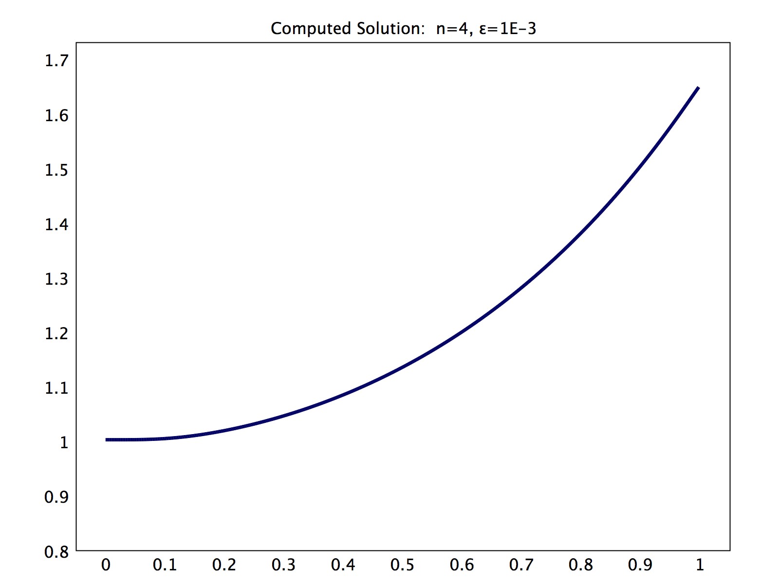
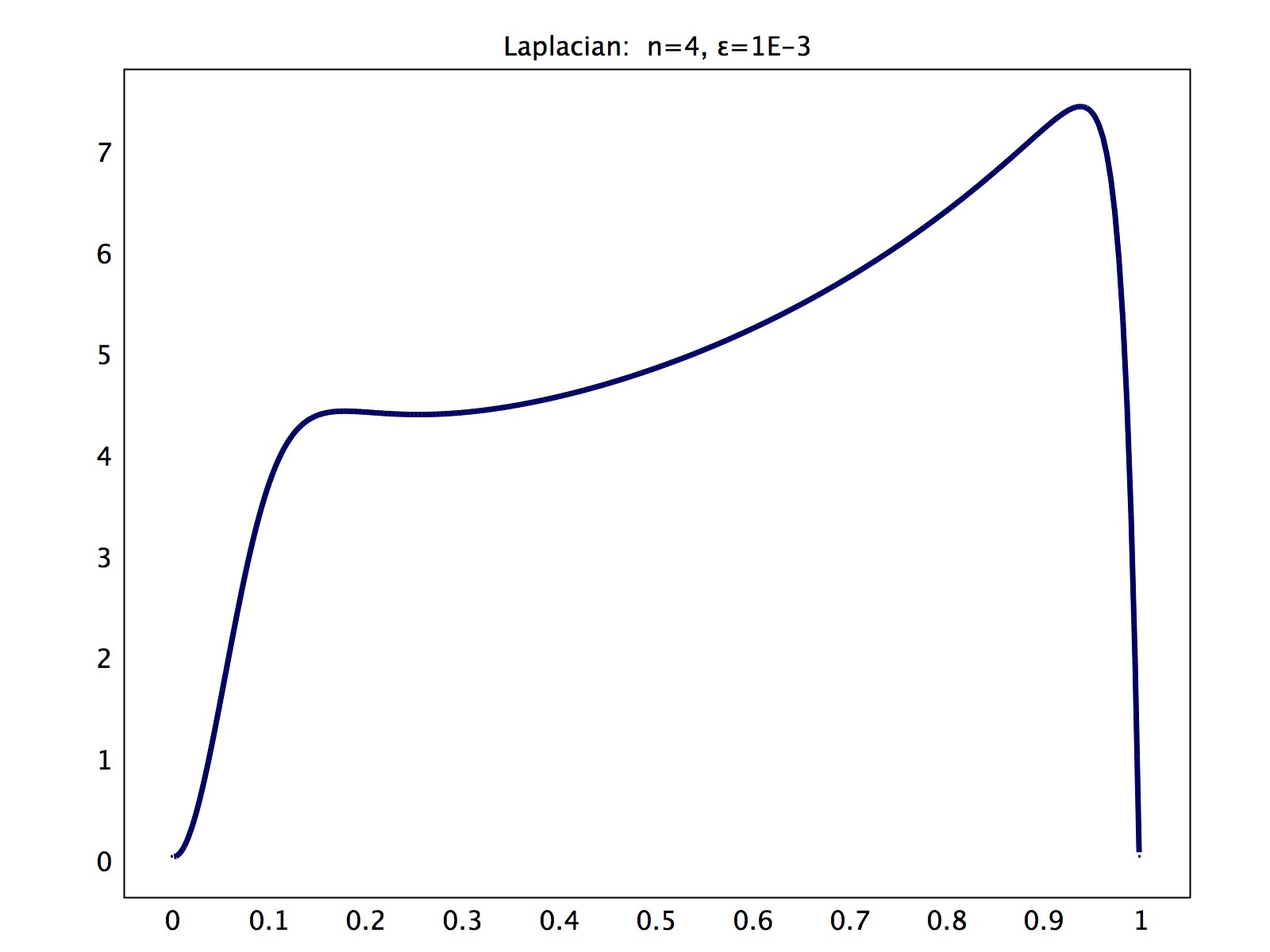
Fig. 1: Computed solution of (8) (left) and and computed Laplacian (right) with $n=4,\varepsilon=10^{-1},h=4\times 10^{-3}$.

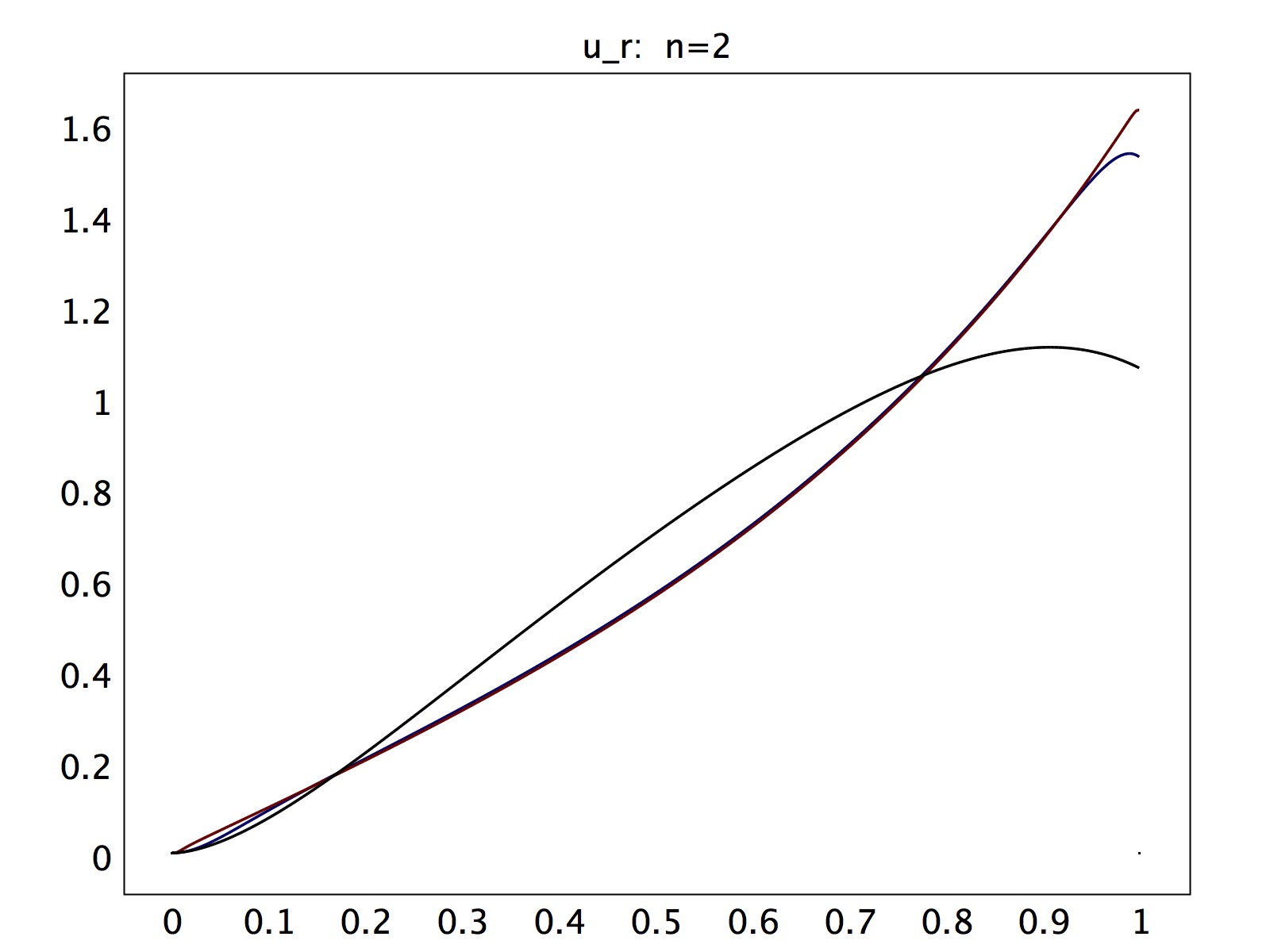
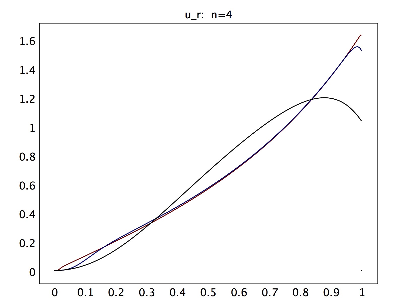
Fig. 2: Computed $u_{r}$ of (8) for $n=2$ (left), and $n=4$ (right) with $\varepsilon=10^{-1}$ (black), $\varepsilon=10^{-3}$ (blue), and $\varepsilon=10^{-5}$ (red) ($h=4\times 10^{-3}$).

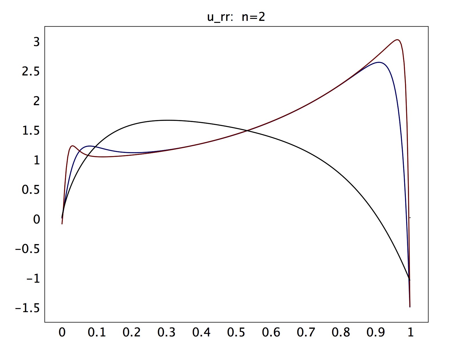
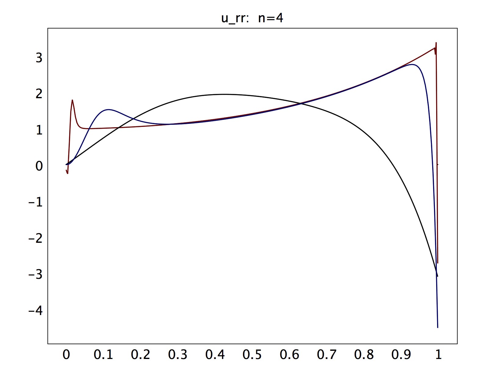
Fig. 3: Computed $u_{rr}$ of (8) for $n=2$ (left), and $n=4$ (right) with $\varepsilon=10^{-1}$ (black), $\varepsilon=10^{-3}$ (blue), and $\varepsilon=10^{-5}$ (red) ($h=4\times 10^{-3}$).

8 Concluding Remarks

We like to comment on an interesting property of the vanishing moment method, namely, the ability of the vanishing moment method to approximate the concave solution of the Monge-Ampère problem (3). This can be achieved simply by letting ${\varepsilon}\nearrow 0^{-}$ in (2). This property can be easily proved as follows in the radially symmetric case.

Before giving the proof, we note that for a given $f>0$ in ${\Omega}$, equation (3a) does not a have concave solution in odd dimensions (i.e., $n$ is odd) because $\mbox{det}(D^{2}u)=f$ does not hold for any concave function $u$ as all $n$ eigenvalues of Hessian $D^{2}u$ of a concave function $u$ must be nonpositive. On the other hand, in even dimensions (i.e., $n$ is even), it is trivial to check that if $u$ is a convex solution of problem (3) with $g=0$, then $-u$, which is a concave function, must also be a solution of problem (3).

Next, by the same token, it is easy to prove that if $u^{\varepsilon}$ is a convex or “almost convex” solution to problem (2), then $-u^{\varepsilon}$, which is concave or “almost concave” in the sense that $-u^{\varepsilon}$ is concave in ${\Omega}$ minus an $O({\varepsilon})$-neighborhood of the boundary ${\partial}{\Omega}$ of ${\Omega}$), must also be a solution of (2).

Finally, let $n$ be a positive even integer, it is easy to see that changing $u^{\varepsilon}$ to $-u^{\varepsilon}$ in (2) is equivalent to changing ${\varepsilon}$ to $-{\varepsilon}$ in (2). For ${\varepsilon}<0$, let $\delta:=-{\varepsilon}$. After replacing ${\varepsilon}$ by $-\delta$ and $u^{\varepsilon}$ by $\hat{u}^{\delta}:=-u^{\varepsilon}$ in (8), we see that $\hat{u}^{\delta}$ satisfies the same set of equations (8) with $\delta(>0)$ in place of ${\varepsilon}$. Hence, by the analysis of Sections 2–6 we know that there exists a monotone increasing solution $\hat{u}^{\delta}$ to problem (8) with ${\varepsilon}$ being replaced by $\delta$, which satisfies all the properties proved in Sections 2–6. Translating all these to $u^{\varepsilon}=-\hat{u}^{\delta}$, we conclude that problem (8) for ${\varepsilon}<0$ has a monotone decreasing solution which is either concave or “almost concave” in $(0,R)$ and converges to the unique concave solution of problem (3) as ${\varepsilon}\nearrow 0^{-}$. In addition, $u^{\varepsilon}$ satisfies the error estimates stated in Theorems 6.1 and 6.3.

References

- [1] A. D. Aleksandrov, Certain estimates for the Dirichlet problem, Soviet Math. Dokl., 1:1151-1154, 1961.
- [2] J.-D. Benamou and Y. Brenier, A computational fluid mechanics solution to the Monge-Kantorovich mass transfer problem, Numer. Math., 84(3):375–393, 2000.
- [3] Y. Brenier, A modified least action principle allowing mass concentrations for the early universe reconstruction problem. preprint.
- [4] S. C. Brenner and L. R. Scott, The Mathematical Theory of Finite Element Methods, third edition, Springer, 2008.
- [5] L. Caffarelli, L. Nirenberg, and J. Spruck, The Dirichlet problem for nonlinear second-order elliptic equations, I. Monge-Ampère equation. Commun. Pure Appl. Math., 37(3):369–402, 1984.
- [6] L. A. Caffarelli and X. Cabré, Fully nonlinear elliptic equations, volume 43 of American Mathematical Society Colloquium Publications. American Mathematical Society, Providence, RI, 1995.
- [7] L. A. Caffarelli and M. Milman, Monge Ampère Equation: Applications to Geometry and Optimization, Contemporary Mathematics, American Mathematical Society, Providence, RI, 1999.
- [8] M. G. Crandall and P.-L. Lions, Viscosity solutions of Hamilton-Jacobi equations, Trans. Amer. Math. Soc., 277(1):1–42, 1983.
- [9] M. G. Crandall, H. Ishii and P.-L. Lions, User’s guide to viscosity solutions of second order partial differential equations, Bull. Amer. Math. Soc. (N.S.), 27(1):1–67, 1992.
- [10] L. C. Evans, Partial Differential Equations, volume 19 of Graduate Studies in Mathematics, American Mathematical Society, Providence, RI, 1998.
- [11] X. Feng, R. Glowinski and M. Neilan, Recent developments in numerical methods for fully nonlinear second order PDEs, to appear in SIAM Review.
- [12] X. Feng and M. Neilan, Vanishing moment method and moment solutions for second order fully nonlinear partial differential equations, J. Scient. Comp., 38(1):74–98, 2009.
- [13] X. Feng and M. Neilan, Mixed finite element methods for the fully nonlinear Monge-Ampère equation based on the vanishing moment method, SIAM J. Numer. Anal., 47(2):1226–1250, 2009.
- [14] X. Feng and M. Neilan, Error Analysis of Galerkin approximations of the fully nonlinear Monge-Ampère equation, J. Sciet. Comp., 47:303–327, 2011.
- [15] W. H. Fleming and H. M. Soner, Controlled Markov Processes and Viscosity Solutions, vol. 25 of Stochastic Modeling and Applied Probability. Springer, New York, second edition, 2006.
- [16] D. Gilbarg and N. S. Trudinger, Elliptic Partial Differential Equations of Second Order, Classics in Mathematics, Springer-Verlag, Berlin, 2001. Reprint of the 1998 edition.
- [17] R. Glowinski, Numerical methods for fully nonlinear elliptic equations, In Proceedings of 6th International Congress on Industrial and Applied Mathematics, R. Jeltsch and G. Wanner, editors, pages 155–192, 2009.
- [18] C. E. Gutierrez, The Monge-Ampère Equation, volume 44 of Progress in Nonlinear Differential Equations and Their Applications, Birkhauser, Boston, MA, 2001.
- [19] B. Guan, On the existence and regularity of hypersurfaces of prescribed Gauss curvature with boundary, Indiana Univ. Math. J. 44(1):21–241, 1995.
- [20] J.-B. Hiriart-Urruty and C. Lemaréchal, Fundamentals of Convex Analysis, Springer, 2001.
- [21] D. Monn, Regularity of the complex Monge-Ampère equation for radially symmetric functions of the unit ball, Math. Ann., 275:501–511, 1986.
- [22] M. Neilan, Numerical Methods for Fully Nonlinear Second Order Partial Differential Equations, Ph.D. Dissertation, The University of Tennessee, 2009.
- [23] M. Neilan, A nonconforming Morley finite element method for the Monge-Ampère equation, Numer. Math., 115(3):371–394, 2010.
- [24] M. H. Protter and H. F. Weinberger, Maximum Principles in Differential Equations, Prentice-Hall, 1967.
- [25] C. Rios and E. T. Sawyer, Smoothness of radial solutions to Monge-Ampère equations, Proc. of AMS, 137:1373–1379, 2008.
- [26] N. S. Trudinger and X.-J. Wang, The Monge-Ampère equation and its geometric applications. In Handbook of geometric analysis. No. 1, volume 7 of Adv. Lect. Math. (ALM), pages 467–524. Int. Press, Somerville, MA, 2008.