Exponentiated Weibull Power Series Distributions and its Applications

Abstract

In this paper we introduce the exponentiated Weibull power series (EWPS) class of distributions which is obtained by compounding exponentiated Weibull and power series distributions, where the compounding procedure follows same way that was previously carried out by Roman et al. (2010) and Cancho et al. (2011) in introducing the complementary exponential-geometric (CEG) and the two-parameter Poisson-exponential (PE) lifetime distributions, respectively. This distribution contains several lifetime models such as: exponentiated weibull-geometric (EWG), exponentiated weibull-binomial (EWB), exponentiated weibull-poisson (EWP), exponentiated weibull-logarithmic (EWL) distributions as a special case.

The hazard rate function of the EWPS distribution can be increasing, decreasing, bathtub-shaped and unimodal failure rate among others. We obtain several properties of the EWPS distribution such as its probability density function, its reliability and failure rate functions, quantiles and moments. The maximum likelihood estimation procedure via a EM-algorithm is presented in this paper. Sub-models of the EWPS distribution are studied in details. In the end, Applications to two real data sets are given to show the flexibility and potentiality of the EWPS distribution.

1 Introduction

The Weibull and exponentiated Weibull (EW) distributions in spite of their simplicity in solving many problems in lifetime and reliability studies, do not provide a reasonable parametric fit to some practical applications.

Recently, attempts have been made to define new families of probability distributions that extend well-known families of distributions and at the same time provide great flexibility in modeling data in practice. One such class of distributions generated by compounding the well-known lifetime distributions such as exponential, Weibull, generalized exponential, exponentiated Weibull and etc with some discrete distributions such as binomial, geometric, zero-truncated Poisson, logarithmic and the power series distributions in general. The non-negative random variable $Y$ denoting the lifetime of such a system is defined by ${{Y=\min}_{1\leq i\leq N}X_{i}\ }$ or ${{Y=\max}_{1\leq i\leq N}X_{i}\ }$, where the distribution of $X_{i}$ belongs to one of the lifetime distributions and the random variable $N$ can have some discrete distributions, mentioned above.

This new class of distributions has been received considerable attention over the last years. The exponential geometric (EG), exponential Poisson (EP), exponential logarithmic (EL), exponential power series (EPS), Weibull geometric (WG), Weibull power series (WPS), exponentiated exponential-Poisson (EEP), complementary exponential geometric (CEG), two-parameter Poisson-exponential, generalized exponential power series (GEPS), exponentiated Weibull-Poisson (EWP) and generalized inverse Weibull-Poisson (GIWP) distributions were introduced and studied by Adamidis and Loukas [2], Kus [17], Tahmasbi and Rezaei [30], Chahkandi and Ganjali [11], Barreto-Souza et al. [7], Morais and Barreto-Souza et al. [23], Barreto-Souza and Cribari-Neto [5], Louzada-Neto et al. [18], Cancho et al. [10], Mahmoudi and Jafari [19], Mahmoudi and Sepahdar [20] and Mahmoudi and Torki [21].

In this paper we introduce the exponentiated Weibull power series (EWPS) class of distributions which is obtained by compounding exponentiated Weibull and power series distributions, where the compounding procedure follows same way that was previously carried out by Roman et al. (2010) and Cancho et al. (2011) in introducing the complementary exponential-geometric (CEG) and the two-parameter Poisson-exponential (PE) lifetime distributions, respectively. This distribution contains several lifetime models such as: exponentiated weibull-geometric (EWG), exponentiated weibull-binomial (EWB), exponentiated weibull-poisson (EWP), exponentiated weibull-logarithmic (EWL) distributions as a special case.

2 Exponentiated Weibull distribution: A brief review

Mudholkar and Srivastava [24] introduced the EW family as extension of the Weibull family, which contains distributions with bathtub-shaped and unimodal failure rates besides a broader class of monotone failure rates. One can see Mudholkar et al. [25], Mudholkar and Huston [26], Gupta and Kundu [15], Nassar and Eissa [28] and Choudhury [13] for applications of the EW distribution in reliability and survival studies.

The random variable $X$ has an EW distribution if its cumulative distribution function (cdf) takes the form

$$G_{X}(x)=\left(1-e^{-(\beta x)^{\gamma}}\right)^{\alpha},~{}~{}x>0,$$ (1)

where $\gamma>0$, $\alpha>0$ and $\beta>0$, which is denoted by $EW(\alpha,\beta,\gamma)$. The corresponding probability density function (pdf) is

$$g_{X}(x)=\alpha\gamma\beta^{\gamma}x^{\gamma-1}e^{-(\beta x)^{\gamma}}\left(1-e^{-(\beta x)^{\gamma}}\right)^{\alpha-1}.$$ (2)

The survival and hazard rate functions of the EW distribution are

$$S(x)=1-\left(1-e^{-(\beta x)^{\gamma}}\right)^{\alpha},$$

and

$$h(x)=\alpha\gamma\beta^{\gamma}x^{\gamma-1}e^{-(\beta x)^{\gamma}}\left(1-e^{-(\beta x)^{\gamma}}\right)^{\alpha-1}\Big{\{}\left[1-\left(1-e^{-(\beta x)^{\gamma}}\right)^{\alpha}\right]\Big{\}}^{-1},$$

respectively. The $k$th moment about zero of the EW distribution is given by

$$E(X^{k})=\alpha\beta^{-k}\Gamma\left(\frac{k}{\gamma}+1\right)\sum_{j=0}^{\infty}(-1)^{j}{\alpha-1\choose j}(j+1)^{-(\frac{k}{\gamma}+1)}.$$ (3)

Note that for positive integer values of $\alpha$, the index $j$ in previous sum stops at $\alpha-1$, and the above expression takes the closed form

$$E(X^{k})=\alpha\beta^{-k}\Gamma\left(\frac{k}{\gamma}+1\right)A_{k}(\gamma),$$ (4)

where

$$A_{k}(\gamma)=1+\sum_{j=1}^{\alpha-1}(-1)^{j}{\alpha-1\choose j}(j+1)^{-(\frac{k}{\gamma}+1)},~{}~{}~{}k=1,2,3,\cdots,$$ (5)

in which $\Gamma(\frac{k}{\gamma}+1)$ denotes the gamma function (see, Nassar and Eissa (2003) for more detail).

Table 1: Useful quantities of some power series distributions.

Distribution	$a‎_{n}$‎	$C(‎\theta‎)$	$C^{\prime‎}(‎\theta‎)$	$C^{\prime\prime}(‎\theta‎)$	$C(‎\theta‎)^{-1}$	$S$
Poisson	$\begin{array}[]{l}n!^{-1}\end{array}$	$e^{‎\theta‎}-1$	$e^{‎\theta‎}$	$e^{‎\theta‎}$	$‎\log‎(‎\theta+1‎)$	$‎\infty‎$
Logarithmic	$\begin{array}[]{l}n^{-1}\end{array}$	$-‎‎\log‎(1-‎\theta‎)$	$‎(1-‎\theta‎)^{-1}$	$‎(1-‎\theta‎)^{-2}$	$1-e^{-‎\theta‎}$	1
Geometric	$\begin{array}[]{l}1\end{array}$	$‎\theta‎‎(1-‎\theta‎)^{-1}$	$‎(1-‎\theta‎)^{-2}$	$2‎(1-‎\theta‎)^{-3}$	$‎\theta‎‎(1+‎\theta‎)^{-1}$	1
Binomial	${m\choose n}$	$‎‎(‎\theta+1‎‎)^{m}-1$	$m‎‎(‎\theta+1‎‎)^{m-1}$	$‎\frac{m(m-1)}{(‎\theta+1‎‎)^{2-m}}‎$	$(‎\theta-1‎)^{‎\frac{1}{m}‎}-1$	$‎\infty‎$

3 The class of EWPS distribution

Consider the random variable $X$ having the EW distribution where its cdf and pdf are given in (1) and (2).
Given $N$, let $X_{1},\cdots,X_{N}$ be independent and identically distributed (iid) random variables from EW distribution. Let the random variable $N$ is distributed according to the power series distribution with pdf

$$P(N=n)=\frac{a_{n}\theta^{n}}{C(\theta)},~{}n=1,2,\cdots,$$

where $a_{n}\geq 0$ depends only on n, $C(\theta)=\Sigma_{n=1}^{\infty}a_{n}\theta^{n}$, $\theta\in(0,s)$ is such that $C(\theta)$ is finite. For more details on the power series class of distributions, see Noack (1950).Table 1 shows useful quantities of some power series distributions (truncated at zero) such as poisson, logarithmic, geometric and binomial (with m being the number of replicas) distributions.
Let $Y=\max(X_{1},\cdots,X_{N})$, then the conditional cdf of $Y|N=n$ is given by

$$G_{Y|N=n}(y)=(G(y))^{n}=\left(1-e^{-(\beta y)^{\gamma}}\right)^{n\alpha},$$ (6)

which is the EW distribution with parameters $n\alpha$, $\beta$, $\gamma$, and denoted by EW$(n\alpha,\beta,\gamma)$. The exponentiated Weibull power series (EWPS) distribution, denoted by EWPS $(\alpha,\beta,\gamma,\theta)$, is defined by the marginal cdf of $Y$, i.e.,

$$F_{Y}(y)=\sum_{n=1}^{\infty}\frac{a_{n}\theta^{n}}{C(\theta)}(G(y))^{n}=\frac{C\left(\theta\left(1-e^{-(\beta y)^{\gamma}}\right)^{\alpha}\right)}{C(\theta)},~{}~{}y>0.$$ (7)

Remark 1

Let $Y=\min(X_{1},\cdots,X_{N})$, then the cdf of $Y$ is given by

$$F_{Y}(y)=1-\frac{C\left(\theta\left(1-e^{-(\beta y)^{\gamma}}\right)^{\alpha}\right)}{C(\theta)},~{}~{}y>0.$$ (8)

If $‎\alpha‎=1$, then the cdf of $Y$ is $F_{Y}(y)=1-\frac{C\left(\theta\left(1-e^{-(\beta y)^{\gamma}}\right)\right)}{C(\theta)}$, which is called Weibull Power Series distributions (Morais and Barreto-Souza, 2011) and this family includes the life time distribution presented by Barreto-Souza et al. (2010a), Barreto-Souza et al. (2010b). which $X_{i}$’s has the exponentiated Weibull distribution is obtained. The EG distribution (Adamidis and Loukas, 1998) is obtained by taking $C(‎\theta‎)=‎\theta‎‎(1-‎\theta‎)^{-1}$ with $‎\theta‎\in(0,1)‎‎$ and $‎\alpha=1,‎\gamma=1‎‎$ in (8). Moreover, for $‎\alpha=1,‎\gamma=1‎‎$, we obtain the EP distribution (Kus, 2007) and the EL distribution (Tahmasbi and Rezaei, 2008) by taking $C(‎\theta‎)=‎e^{‎\theta‎}-1,‎\theta‎\>0‎‎$, and $C(‎\theta‎)=‎-‎‎\log‎(1-‎\theta‎),\theta‎\in(0,1)$, respectively. The WG distribution (Barreto-Souza et al. (2010a), Barreto-Souza et al. (2010b) ) is obtained by taking $C(‎\theta‎)=‎\theta‎‎(1-‎\theta‎)^{-1}$ with $‎\theta‎\in(0,1)‎‎$ and $‎\alpha=1‎$ in (8). The EWG distribution is obtained by considering $C(‎\theta‎)=‎\theta‎‎(1-‎\theta‎)^{-1}$ with $‎\theta‎\in(0,1)‎‎$ in (8).

The pdf of the EWPS distribution is given by

$$f_{Y}(y)=\theta\alpha\gamma\beta^{\gamma}y^{\gamma-1}e^{-(\beta y)^{\gamma}}\left(1-e^{-(\beta y)^{\gamma}}\right)^{\alpha-1}\frac{C^{\prime}\left(\theta\left(1-e^{-(\beta y)^{\gamma}}\right)^{\alpha}\right)}{C(\theta)},$$ (9)

where $\alpha,\beta,\gamma>0$ and $\theta\in(0,s)$.
The survival function and hazard rate function of the EWPS distribution are given, respectively, by

$$S(y)=1-\frac{C\left(\theta\left(1-e^{-(\beta y)^{\gamma}}\right)^{\alpha}\right)}{C(\theta)},~{}~{}y>0,$$ (10)

and

$$h(y)=\theta\alpha\gamma\beta^{\gamma}y^{\gamma-1}e^{-(\beta y)^{\gamma}}\left(1-e^{-(\beta y)^{\gamma}}\right)^{\alpha-1}\frac{C^{\prime}\left(\theta\left(1-e^{-(\beta y)^{\gamma}}\right)^{\alpha}\right)}{C(\theta)-C\left(\theta\left(1-e^{-(\beta y)^{\gamma}}\right)^{\alpha}\right)}.$$ (11)

Consider $C(\theta)=‎\theta+‎\theta‎^{20}‎‎‎$. If $‎‎\beta=1‎‎$ and $‎\theta=1‎$, the plots of this density and its hazard rate function, for $‎\alpha=0.5,‎\gamma=1,‎\alpha=1,‎\gamma=0.5,‎\alpha=2,‎\gamma=3,$ and $‎\alpha=2,‎\gamma=1$ are given in Fig 1.

Proposition 1

The limiting distribution of $EWPS(‎\alpha,‎\beta,‎\gamma,‎\theta‎‎‎‎)$ when $‎\theta‎\rightarrow 0^{+}‎‎$ is

$$\begin{array}[b]{ll}\lim‎_{\theta‎\rightarrow 0^{+}}‎‎‎F(y)&=\lim‎_{\theta‎\rightarrow 0^{+}}‎\frac{C(\theta G(y))}{C(\theta)}=\lim‎_{\theta‎\rightarrow 0^{+}}‎\frac{\sum_{n=1}^{\infty}a_{n}‎\theta^{n}(G(y))^{n}‎}{\sum_{n=1}^{\infty}a_{n}‎\theta^{n}}\vskip 6.0pt plus 2.0pt minus 2.0pt\\ &=‎\lim‎_{\theta‎\rightarrow 0^{+}}‎‎\frac{a_{c}(G(y))^{c}+\sum_{n=c+1}^{\infty}a_{n}‎\theta^{n-c}(G(y))^{n}}{a_{c}+\sum_{n=c+1}^{\infty}a_{n}‎\theta^{n-c}}‎\vskip 6.0pt plus 2.0pt minus 2.0pt\\ &=(G(y))^{c}=\left(1-e^{-(\beta y)^{\gamma}}\right)^{c\alpha}\end{array}$$

which is a EW distribution with parameters $c‎\alpha‎$, $‎\gamma‎$ and $‎\beta‎$, where $c=min‎\{‎n‎\in N‎:a_{n}‎\>0‎‎\}‎$.

Proposition 2

The densities of EWPS class can be expressed as infinite linear combination of density of order distribution. We know that

$$C^{\prime}(\theta)=\Sigma_{n=1}^{\infty}na_{n}\theta^{n-1}$$

.
Therefore,

$$f_{Y}(y)=\theta\alpha\gamma\beta^{\gamma}y^{\gamma-1}e^{-(\beta y)^{\gamma}}\left(1-e^{-(\beta y)^{\gamma}}\right)^{\alpha-1}\sum_{n=1}^{\infty}\frac{na_{n}}{C(\theta)}\left(\theta\left(1-e^{-(\beta y)^{\gamma}}\right)^{\alpha}\right)^{n-1}.$$

Using the EW density given before, we obtain

$$f_{EWPS}(y;\alpha,\beta,\gamma,\theta)=\theta\sum_{n=1}^{\infty}\frac{\theta^{n-1}a_{n}}{C(\theta)}f_{EW}(y;n\alpha,\beta,\gamma).$$ (12)

Various mathematical properties (cdf, moments, percentiles, moment‎•‎ generating function, factorial moments, among others) of the EWPS distribution for $|\theta|<1$ can be obtained from Eq. (12) and the corresponding properties of the EW distribution.

Proposition 3

The density of EWPS distribution can be expressed as infinite linear combination of density of the biggest order statistic of $X_{1},\cdots,X_{n}$, where $X_{i}\sim EW(\alpha,\beta,\gamma)$ for $i=1,2,\cdots,n$. we have

$$f_{EWPS}(y)=\sum^{\infty}_{n=1}(G(y))^{n}P(N=n)=\sum^{\infty}_{n=1}g_{X_{(n)}}(y)P(N=n),$$

in which $g_{X_{(n)}}(y)$ is the pdf of $X_{(n)}=\max(X_{1},\cdots,X_{n})$.

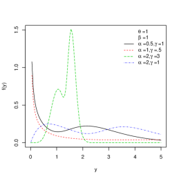
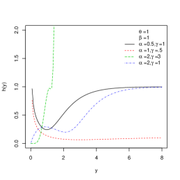
Figure 1: Plots of pdf and hazard rate function of EWPS where $C(\theta)=‎\theta+‎\theta^{20}‎‎$.

‎‎‎‎‎

4 Quantiles and moments of the EWPS distribution

The $q$th quantile of the EWPS distribution is given by

$$y_{q}=G^{-1}\left(\frac{C^{-1}(qC(\theta)}{\theta}\right),$$

Where $G^{-1}(y)=\frac{1}{\beta}\left(-\ln\left(1-y^{\frac{1}{\alpha}}\right)\right)^{\frac{1}{\gamma}}$, and $C^{-1}(.)$ is the inverse function of $C(.)$. The $q$th quantile of the EWPS distribution is used for data generation from the EWPS distribution. In particular, the median of the EWPS distribution is given by

$$y_{0.5}=G^{-1}\left(\frac{C^{-1}(0.5C(\theta))}{\theta}\right).$$

Suppose that $Y\sim EWPS(\alpha,\beta,\gamma,\theta)$, and $X_{(n)}=\max(X_{1},\cdots,X_{n})$, where $X_{i}\sim EW(\alpha,\beta,\gamma)$ for $i=1,2,\cdots,n$, then the $k$th moment of $Y$ is given by

$$\begin{array}[b]{ll}E(Y^{k})=E(E(Y^{k}|N))&=\sum^{\infty}_{n=1}P(N=n)E(Y^{k}|n)=\sum^{\infty}_{n=1}P(N=n)E(X^{k}_{(n)})\vskip 6.0pt plus 2.0pt minus 2.0pt\\ &=\alpha\beta^{-k}\Gamma\left(\frac{k}{\gamma}+1\right)\sum^{\infty}_{n=1}\sum^{\infty}_{j=0}(-1)^{j}\frac{a_{n}\theta^{n}}{C(\theta)}{n\alpha-1\choose j}n(j+1)^{-(\frac{k}{\gamma}+1)}.\end{array}$$ (13)

For positive integer values of $\alpha$, the index $j$ in above expression stops at $n\alpha-1$

Now we obtain the moment generating function of the EWPS distribution using the Eq. (13), as follow

$$\begin{array}[b]{l}M_{Y}(t)=\sum^{\infty}_{i=0}\frac{t^{i}}{i!}E(Y^{i})\vskip 6.0pt plus 2.0pt minus 2.0pt\\ =\sum^{\infty}_{i=0}\frac{t^{i}}{i!}\left[(1-\theta)\alpha\beta^{-i}\Gamma\left(\frac{i}{\gamma}+1\right)\sum^{\infty}_{n=1}\sum^{\infty}_{j=0}(-1)^{j}{n\alpha-1\choose j}n\theta^{n-1}(j+1)^{-(\frac{i}{\gamma}+1)}\right]\vskip 6.0pt plus 2.0pt minus 2.0pt\\ =\sum^{\infty}_{i=0}\sum^{\infty}_{n=1}\sum^{\infty}_{j=0}‎\frac{(-1)^{j}}{i!}‎(t/\beta)^{i}\frac{a_{n}\theta^{n}}{C(\theta)}{n\alpha-1\choose j}‎\frac{‎n‎\alpha‎\Gamma\left(\frac{i}{\gamma}+1\right)}{(j+1)^{-(\frac{i}{\gamma}+1)}}.\end{array}$$ (14)

According to the Eq. (13), the mean and variance of the EWPS distribution are given, respectively, by

$$E(Y)=\alpha\beta^{-1}\Gamma\left(\frac{1}{\gamma}+1\right)\sum^{\infty}_{n=1}\sum^{\infty}_{j=0}(-1)^{j}\frac{a_{n}\theta^{n}}{C(\theta)}{n\alpha-1\choose j}n(j+1)^{-(\frac{1}{\gamma}+1)},$$ (15)

and

$$Var(Y)=\alpha\beta^{-2}\Gamma\left(\frac{2}{\gamma}+1\right)\sum^{\infty}_{n=1}\sum^{\infty}_{j=0}(-1)^{j}\frac{a_{n}\theta^{n}}{C(\theta)}{n\alpha-1\choose j}n(j+1)^{-(\frac{2}{\gamma}+1)}-E^{2}(Y),$$ (16)

Where $E(Y)$ is given in Eq. (15)

5 Rényi and Shannon entropies

Entropy has been used in various situations in science and engineering. The entropy of a random $Y$ is a measure of variation of the uncertainty. For a random variable with the pdf $f$, the Rényi entropy is defined by $I_{R}(r)=\frac{1}{1-r}\log\{\int_{\mathbb{R}}f^{r}(y)dy\}$, for $r>0$ and $r\neq 1$. For the EWPS distribution, the power series expansion gives

$$\begin{array}[b]{ll}\int^{\infty}_{0}f^{r}(y)dy&=\left[\frac{\alpha\theta\gamma\beta^{\gamma}}{C(\theta)}\right]^{r}\int^{\infty}_{0}e^{-r(\beta y)^{\gamma}}(1-e^{-(\beta y)^{\gamma}})^{r\alpha-r}‎\frac{‎\left[C‎^{\prime}‎(‎\theta(1-e^{-(\beta y)^{\gamma}})^{\alpha}‎‎)‎‎\right]‎^{r}‎‎}{‎\left[‎C(‎\theta‎)‎\right]‎^{r}‎‎}‎dy\end{array},$$

Applying the Equation $‎\left(‎\sum^{\infty}_{i=0}w‎_{i}u‎^{i}‎‎\right)‎^{j}‎‎=‎\sum^{\infty}_{i=0}c‎_{i,j}u‎^{i}‎$, where the coefficients $c‎_{i,j}$ for $i=1,2,...$ can be easily obtained from the recurrence relation $c‎_{i,j}=(iw‎_{0}‎)‎^{-1}‎\sum^{i}_{m=1}(jm-i+m)w‎_{m}c‎_{i-m,j},$ white $c‎_{0,j}=w‎_{0}‎^{j}‎$ for $‎\left[C‎^{\prime}‎(‎\theta(1-e^{-(\beta y)^{\gamma}})^{\alpha}‎‎)‎‎\right]‎^{r}‎$and series expansion for $\left(1-(1-e^{-(\beta x)^{\gamma}})^{\alpha}\right)^{-(r+2)}$ gives

$$\begin{array}[b]{ll}\int^{\infty}_{0}f^{r}(y)dy&=\left[\frac{\alpha\theta\gamma\beta^{\gamma}}{C(\theta)}\right]^{r}\sum^{\infty}_{i=0}\sum^{\infty}_{j=0}(-1)‎^{j}‎c‎_{i,j}‎\theta‎^{i}{\alpha(r+i)-r\choose j}‎‎\int^{\infty}_{0}e^{-(r+j)(\beta y)^{\gamma}}dy\end{array},$$

But setting $u=(j+r)(\beta y)^{\gamma}$, gives

$$\begin{array}[b]{ll}\int^{\infty}_{0}f^{r}(y)dy&=\left[\frac{\alpha\theta}{C(\theta)}\right]^{r}‎\gamma‎^{r-1}‎‎\beta^{r\gamma-1}\Gamma(\frac{1}{\gamma})\sum_{i=0}^{\infty}\sum_{j=0}^{\infty}c‎_{i,j}‎\frac{‎(-1)^{j}\theta^{i}}{(j+r)^{\frac{1}{\gamma}}}{\alpha(r+i)-r\choose j}\end{array}.$$ (17)

Substituting from (17), we obtain

$$I_{R}(r)=\frac{1}{1-r}\log\left\{\left[\frac{\alpha\theta}{C(\theta)}\right]^{r}‎\gamma‎^{r-1}‎‎\beta^{r\gamma-1}\Gamma(\frac{1}{\gamma})\sum_{i=0}^{\infty}\sum_{j=0}^{\infty}c‎_{i,j}‎\frac{‎(-1)^{j}\theta^{i}}{(j+r)^{\frac{1}{\gamma}}}{\alpha(r+i)-r\choose j}\right\}.$$ (18)

The Shannon entropy which is defined by $E[-\log(f(Y))]$, is derived from $\lim_{r\rightarrow 1}I_{R}(r)$.

6 Moments of order statistics

Order statistics make their appearance in many areas of statistical theory and practice. Let the random variable $Y_{r:n}$ be the $r$th order statistic $(Y_{1:n}\leq Y_{2:n}\leq\cdots\leq Y_{n:n})$ in a sample of size $n$ from the EWPS distribution. The pdf of $Y_{r:n}$ for $r=1,\cdots,n$, is given by

$$f_{r:n}(y)=\frac{1}{B(r,n-r+1)}f(y)F(y)^{r-1}[1-F(y)]^{n-r},~{}~{}~{}y>0.$$ (19)

where $F(y)$ and f(y) are given in (7) and (9). Substituting from (7) and (9) into (19) gives

$$\begin{array}[b]{ll}f_{r:n}(y)&=\frac{\alpha\theta\gamma\beta^{\gamma}}{B(r,n-r+1)C(\theta)^{n}}y^{\gamma-1}e^{-(\beta y)^{\gamma}}(1-e^{-(\beta y)^{\gamma}})^{\alpha-1}C^{\prime}(\theta(1-e^{-(\beta y)^{\gamma}})^{\alpha})\\ &(C(\theta(1-e^{-(\beta y)^{\gamma}})^{\alpha}))^{r-1}(C(\theta)-C(\theta(1-e^{-(\beta y)^{\gamma}})^{\alpha}))^{n-r},\end{array}$$ (20)

Also the cdf of $Y_{r:n}$ is given by

$$\begin{array}[b]{ll}F_{r:n}(y)&=\sum^{n}_{k=r}{{n}\choose{k}}[F(y)]^{k}[1-F(y)]^{n-k}\vskip 6.0pt plus 2.0pt minus 2.0pt\\ &=\sum^{n}_{k=r}{{n}\choose{k}}\frac{(C(\theta(1-e^{-(\beta y)^{\gamma}})^{\alpha}))^{k}(C(\theta)-C(\theta(1-e^{-(\beta y)^{\gamma}})^{\alpha}))^{n-k}}{C(\theta)^{n}}.\end{array}$$ (21)

Expression for the rth moment of the order statistics $(Y_{1:n}\leq Y_{2:n}\leq\cdots\leq Y_{n:n})$, with a cdf in the form (21), are obtained by using a result due to Barakat and Abdelkader (2004) and becomes

$$\begin{array}[b]{ll}E(Y_{r:n}^{k})&=k\sum^{\infty}_{j=n-r+1}(-1)^{j-n+r-1}{{j-1}\choose{n-r}}{{n}\choose{j}}\int^{\infty}_{0}y^{k-1}S(y)^{j}dy\vskip 6.0pt plus 2.0pt minus 2.0pt\\ &=k\sum^{\infty}_{j=n-r+1}\sum^{\infty}_{s=0}\frac{(-1)^{j-n+r+s-1}}{C(\theta)^{s}}{{j-1}\choose{n-r}}{{n}\choose{j}}{{j}\choose{s}}\int^{\infty}_{0}y^{k-1}C(\theta(1-e^{-(\beta y)^{\gamma}})^{\alpha})^{s}dy.\end{array}$$ (22)

7 Residual life function of the EWPS distribution

Given that a component survives up to time $t\geq 0$, the residual life is the period beyond $t$ until the time of failure and defined by the conditional random variable $X|X>t$. In reliability, it is well known that the mean residual life function and ratio of two consecutive moments of residual life determine the distribution uniquely (Gupta and Gupta, 1983). Therefore, we obtain the $r$th order moment of the residual life via the general formula

$$m_{r}(t)=E\left[(Y-t)^{r}|Y>t\right]=\frac{1}{S(t)}\int_{t}^{\infty}(y-t)^{r}f(y)dy,$$

where $S(t)=1-F(t)$, is the survival function.
Applying series expansion (9), the binomial expansion to $(y-t)^{r}$ and substituting $S(t)$ given by (10) into the above formula gives the $r$th order moment of the residual life of the EWPS as

$$\begin{array}[b]{ll}m_{r}(t)&=\frac{\alpha}{C(\theta)-C\left(\theta\left(1-e^{-(\beta t)^{\gamma}}\right)^{\alpha}\right)}\sum_{i=0}^{r}\sum_{n=1}^{\infty}\sum_{j=0}^{\infty}\frac{(-1)^{i+j}t^{i}na_{n}\theta^{n}}{(j+1)^{\frac{r+\gamma-i}{\gamma}}\beta^{r-i}}{{n\alpha-1}\choose{j}}\\ &~{}~{}\times‎\Phi‎\left(\frac{r+\gamma-i}{\gamma};(j+1)(\beta t)^{\gamma}\right),~{}~{}~{}r\geq 1,\end{array}$$ (23)

where $‎\Phi‎(s;t)$ is the upper incomplete gamma function given by $‎\Phi‎(s;t)=\int_{t}^{\infty}x^{s-1}e^{-x}dx$.
Another important representation for the EWPS is the mean Residual life (MRL) function obtain by setting $r=1$ in Eq. (23). MRL function as well as failure rate (FR) function is very important since each of them can be used to determine a unique corresponding life time distribution. Life times can exhibit IMRL (increasing MRL) or DMRL (decreasing MRL). MRL functions that first decreases (increases) and then increases (decreases) are usually called bathtub (upside-down bathtub) shaped, BMRL (UMRL). The relationship between the behaviors of the two functions of a distribution was studied by many authors such as Ghitany (1998), Mi (1995), Park (1985), Shanbhag (1970), and Tang et al. (1999). For the EWPS distribution the MRL function is given in the following theorem.

Theorem 1

The MRL function of the EWPS distribution with cdf (7) is

$$m(t)=(\mu_{1}+I(t)-t)/S(t),~{}~{}t\geq 0$$ (24)

where $I(t)=\int^{t}_{0}F(y)dy$, $S(t)$ is the survival function given in (10), and $\mu_{1}$ is the mean of the EWPS in Eq. (15).

Proof 1

For more detail about the proof of this theorem see Nassar and Eissa (2003).

According to Theorem 1, for the EWPS distribution with $f(y)$ given by (9), we have

$$I(t)=\frac{1}{\beta\gamma C(\theta)}\sum_{n=1}^{\infty}\sum_{k=0}^{\infty}\frac{(-1)^{k}a_{n}\theta^{n}}{k^{\frac{1}{\gamma}}}{{\alpha n}\choose{k}}\Psi(1/\gamma;l(\beta t)^{\gamma}),$$ (25)

where $\Psi(s;t)$ is the lower incomplete gamma function given by $\Psi(s;t)=\int_{0}^{t}x^{s-1}e^{-x}dx$. Substituting Eqs. (15), (15) and (25) into (24) gives the MRL function of the EWPS distribution.

$$\begin{array}[b]{ll}m‎_{1}‎(t)&=\frac{1}{C(\theta)‎\beta‎}\sum_{n=1}^{\infty}\sum_{k=0}^{\infty}‎\frac{(-1)^{k}a_{n}\theta^{n}}{s(t)}‎‎\left[{{n\alpha-1}\choose{k}}‎\frac{n‎\alpha‎‎\Gamma(1+\frac{1}{\gamma})}{(k+1)‎^{1+‎\frac{1}{‎\gamma‎}‎}‎}‎‎‎-{{n\alpha}\choose{k}}e^{-k(\beta t)^{\gamma}}‎‎t+{{n\alpha}\choose{k}}‎\frac{‎\Psi‎(\frac{1}{\gamma},k(‎\beta t‎)‎^{‎\gamma‎}‎)}{k‎^{‎\frac{1}{‎\gamma‎}‎}‎\gamma‎‎}\right]-t\end{array}$$

8 Reversed residual life function of the EWPS distribution

Given that a component survives up to time $t\geq 0$, the residual life is the period beyond $t$ until the time of failure and defined by the conditional random variable $X|X>t$.Therefore, we obtain the $r$th order moment of the residual life via the general formula

$$m_{r}(t)=E\left[(Y-t)^{r}|Y>t\right]=\frac{1}{F(t)}\int_{t}^{\infty}(y-t)^{r}f(y)dy,$$

where $F(t)$, is The exponentiated Weibull power series (EWPS) distribution.
Applying series expansion (9), the binomial expansion to $(t-y)^{r}$ and substituting $F(t)$ given by (7) into the above formula gives the $r$th order moment of the reversed residual life of the EWPS as

$$\begin{array}[b]{ll}M{r}(t)&=\frac{\alpha}{F(t)}\sum_{i=0}^{r}\sum_{n=1}^{\infty}\sum_{j=0}^{\infty}\frac{(-1)^{i+j}t^{r-i}na_{n}\theta^{n}}{(j+1)^{1+\frac{i}{\gamma}}C(‎\theta‎)\beta^{i}}{{n\alpha-1}\choose{j}}\\ &~{}~{}\times‎\Psi‎‎\left(1+\frac{i}{\gamma};(j+1)(\beta t)^{\gamma}\right),~{}~{}~{}r\geq 1,\end{array}$$ (26)

where $‎\Phi‎(s;t)$ is the upper incomplete gamma function given by $‎\Phi‎(s;t)=\int_{t}^{\infty}x^{s-1}e^{-x}dx$.

9 Probability weighted moments

Probability weighted moments (PWMs) are expectations of certain functions of a random variable defined when the ordinary moments of the random variable exist. The probability weighted moments method can generally be used for estimating parameters of a distribution whose inverse form cannot be expressed explicitly. We calculate the PWMs of the EWPS distribution since they can be used to obtain the ordinary moments of the EWPS distribution.

The PWMs of a random variable $X$ are formally defined by

$$\tau_{s,r}=E[X^{s}F(X)^{r}]=\int_{0}^{\infty}x^{s}F(x)^{r}f(x)dx,$$ (27)

where $r$ and $s$ are positive integers and $F(x)$ and $f(x)$ are the cdf and pdf of the random variable $X$. The following theorem gives the PWMs of the EWPS distribution.

Theorem 2

The PWMs of the EWPS distribution with cdf (7) and pdf (9), are given by

$$\tau_{s,r}=‎\frac{‎\alpha‎\theta\Gamma(1+\frac{s}{\gamma})}{‎\beta^{s}(C(‎\theta‎))‎^{r+1}‎}\sum^{\infty}_{n=1}\sum^{\infty}_{i=0}\sum^{\infty}_{j=0}(-1)^{j}‎\frac{na‎_{n}‎\theta‎^{i+n-1}‎‎‎}{(j+1)^{1+\frac{s}{\gamma}}}‎{\alpha(n+i)-1\choose j}.$$ (28)

Proof 2

Substituting from (7) and (9) into (27) gives

$$\tau_{s,r}=‎\frac{\alpha\gamma‎\theta‎\beta^{\gamma}}{(C(‎\theta‎))‎^{r+1}}‎\int\limits_{0}^{\infty}x^{s+\gamma-1}e^{-(\beta x)^{\gamma}}(1-e^{-(\beta x)^{\gamma}})^{\alpha-1}C‎^{\prime}(\theta(1-e^{-(\beta x)^{\gamma}})^{\alpha})‎(C(\theta(1-e^{-(\beta x)^{\gamma}})^{\alpha}))‎^{r}‎dx.$$

Applying the Equation $‎\left(‎\sum^{\infty}_{i=0}w‎_{i}u‎^{i}‎‎\right)‎^{j}‎‎=‎\sum^{\infty}_{i=0}c‎_{i,j}u‎^{i}‎$, where the coefficients $c‎_{i,j}$ for $i=1,2,...$ can be easily obtained from the recurrence relation $c‎_{i,j}=(iw‎_{0}‎)‎^{-1}‎\sum^{i}_{m=1}(jm-i+m)w‎_{m}c‎_{i-m,j},$ white $c‎_{0,j}=w‎_{0}‎^{j}‎$ for $‎\left[C‎^{\prime}‎(‎\theta(1-e^{-(\beta y)^{\gamma}})^{\alpha}‎‎)‎‎\right]‎^{r}‎$and series expansion for $\left(1-(1-e^{-(\beta x)^{\gamma}})^{\alpha}\right)^{-(r+2)}$ gives

$$\tau_{s,r}=‎\frac{\alpha\gamma‎\theta‎\beta^{\gamma}}{(C(‎\theta‎))‎^{r+1}}\sum^{\infty}_{n=1}\sum^{\infty}_{i=0}\sum^{\infty}_{j=0}(-1)‎^{j}‎na‎_{n}‎‎\theta‎^{i+n-1}{\alpha(n+i)-1\choose j}‎‎\int\limits_{0}^{\infty}x^{s+\gamma-1}e^{-(j+1)(\beta x)^{\gamma}}dx.$$

Setting $u=(j+1)(\beta x)^{\gamma}$ the above integral reduces to

$$\int\limits_{0}^{\infty}x^{s+\gamma-1}e^{-(k+1)(\beta x)^{\gamma}}dx=\frac{1}{\gamma\beta^{\gamma+s}(k+1)^{1+\frac{s}{\gamma}}}\Gamma(1+\frac{s}{\gamma}),$$

and the proof is completed.

Remark 2

The sth moment of EWPS distribution can be obtained by putting $r=0$ in Eq. (28). Therefore

$$E(X^{s})=\alpha(1-\theta)\beta^{-s}\Gamma(\frac{s}{\gamma}+1)\sum^{\infty}_{j=0}\sum^{\infty}_{k=0}(-1)^{k}(j+1){\alpha(j+1)-1\choose k}(k+1)^{-(\frac{s}{\gamma}+1)}\theta^{j},$$

which is equal with Eq. (13) if $s$ is replaced by $k$. Also, the mean and variance of the EWPS distribution can be obtained.

10 Mean deviations

The amount of scatter in a population can be measured by the totality of deviations from the mean and median. For a random variable $X$ with pdf $f(.)$, cdf $F(.)$, mean $\mu=E(X)$ and $M=Median(X)$ the mean deviation about the mean and the mean deviation about the median, respectively, are defined by

$$\delta_{1}(X)=\int_{0}^{\infty}|x-\mu|f(x)dx=2\mu F(\mu)-2\mu+2L(\mu),$$

and

$$\delta_{2}(X)=\int_{0}^{\infty}|x-M|f(x)dx=2MF(M)-M-\mu+2L(M),$$

where $L(\mu)=\int^{\infty}_{\mu}xf(x)dx$ and $L(M)=\int^{\infty}_{M}xf(x)dx.$

For the EWPS distribution we have

$$L(b)=\alpha\beta^{-1}\sum^{\infty}_{n=1}\sum^{\infty}_{j=0}(-1)^{j}\frac{na_{n}\theta^{n}}{C(\theta)}{{n\alpha-1}\choose{j}}(j+1)^{-(\frac{1}{\gamma}+1)}‎\Phi‎\left((\frac{1}{1+\gamma});(j+1)(\beta b)^{\gamma}\right).$$ (29)

Theorem 3

The Mean deviations of the EWPS distribution are

$$\delta_{1}=2\mu\left(\frac{C\left(\theta\left(1-e^{-(\beta\mu)^{\gamma}}\right)^{\alpha}\right)-C(\theta)}{C(\theta)}\right)+2L(\mu),$$

and

$$\delta_{2}=2L(M)-\mu,$$

respectively, where $\mu$ is the mean of EWPS in Eq. (15), $L(\mu)$ and $L(M)$ are obtained by substituting $\mu$ and $M=G^{-1}\left(\frac{C^{-1}(0.5C(\theta))}{\theta}\right)$ instead of $b$ in Eq. (29).

11 Bonferoni and Lorenz curves

The Bonferroni and Lorenz curves and Gini index have many applications not only in economics to study income and poverty, but also in other fields like reliability, medicine and insurance. The Bonferroni curve $B_{F}[F(x)]$ is given by

$$B_{F}[F(x)]=\frac{1}{\mu F(x)}\int^{x}_{0}uf(u)du.$$

The Bonferroni curve of the EWPS distribution is given by

$$\begin{array}[]{ll}B_{F}[F(x)]=\frac{\alpha\beta^{-1}}{\mu C\left(\theta\left(1-e^{-(\beta x)^{\gamma}}\right)^{\alpha}\right)}\sum^{\infty}_{n=1}\sum^{\infty}_{j=0}na_{n}\theta^{n}(-1)^{j}{{n\alpha-1}\choose{j}}&\\ ~{}~{}~{}~{}~{}~{}~{}~{}~{}~{}~{}~{}~{}~{}~{}\times(j+1)^{-(\frac{1}{\gamma}+1)}\Psi\left((\frac{1}{\gamma}+1);(j+1)(x\beta)^{\gamma}\right).&\end{array}$$

Also, the Lorenz curve of EWPS distribution can be obtained via the expression

$$\begin{array}[]{ll}L_{F}[F(x)]=\frac{\alpha\beta^{-1}}{\mu C(\theta)}\sum^{\infty}_{n=1}\sum^{\infty}_{j=0}na_{n}\theta^{n}(-1)^{j}{{n\alpha-1}\choose{j}}&\\ ~{}~{}~{}~{}~{}~{}~{}~{}~{}~{}~{}~{}~{}~{}~{}\times(j+1)^{-(\frac{1}{\gamma}+1)}\Psi\left((\frac{1}{\gamma}+1);(j+1)(x\beta)^{\gamma}\right).&\end{array}$$

The scaled total time on test transform of a distribution function $F$ (Pundir et al., 2005) is defined by

$$S_{F}[F(t)]=\frac{1}{\mu}\int^{t}_{0}\bar{F}(u)du.$$

If $F(t)$ denotes the cdf of EWPS distribution then

$$S_{F}[F(t)]=\frac{t}{\mu}-\frac{\beta^{-1}}{\mu\gamma C(\theta)}\sum^{\infty}_{n=1}\sum^{\infty}_{j=0}(-1)^{j}\frac{a_{n}\theta^{n}}{(j)^{(\frac{1}{\gamma})}}{{n\alpha}\choose{j}}\Psi\left(\frac{1}{\gamma};j(t\beta)^{\gamma}\right).$$

The cumulative total time can be obtained by using formula $C_{F}=\int_{0}^{1}S_{F}[F(t)]f(t)dt$ and the Gini index can be derived from the relationship $G=1-C_{F}$.

12 Estimation and inference

In what follows, we discuss the estimation of the parameters for the EWPS distribution. Let $Y_{1},Y_{2},\cdots,Y_{n}$ be a random sample with observed values $y_{1},y_{2},\cdots,y_{n}$ from EWPS distribution with parameters $\alpha,\beta,\gamma$ and $\theta$. Let $\Theta=(\alpha,\beta,\gamma,\theta)^{T}$ be the parameter vector. The total log-likelihood function is given by

$$\begin{array}[b]{ll}l_{n}\equiv l_{n}(y;\Theta)&=n[\log\alpha+\log\gamma+\gamma\log\beta+\log\theta]+(\gamma-1)\sum^{n}_{i=1}\log y_{i}-\sum^{n}_{i=1}(\beta y_{i})^{\gamma}\vskip 6.0pt plus 2.0pt minus 2.0pt\\ &~{}~{}~{}+(\alpha-1)\sum^{n}_{i=1}\log(1-e^{-(\beta y_{i})^{\gamma}})-n\log C(\theta)+\sum^{n}_{i=1}\log[C^{\prime}(\theta\left(1-e^{-(\beta y_{i})^{\gamma}}\right)^{\alpha})].\end{array}$$

The associated score function is given by $U_{n}(\Theta)=(\partial l_{n}/\partial\alpha,\partial l_{n}/\partial\beta,\partial l_{n}/\partial\gamma,\partial l_{n}/\partial\lambda)^{T}$, where

$$\begin{array}[]{ll}\frac{\partial l_{n}}{\partial\alpha}&=\frac{n}{\alpha}+\sum^{n}_{i=1}\log(1-e^{-(\beta y_{i})^{\gamma}})+\theta\sum^{n}_{i=1}\log(1-e^{-(\beta y_{i})^{\gamma}})(1-e^{-(\beta y_{i})^{\gamma}})^{\alpha}~{}\frac{C^{\prime\prime}(\theta(1-e^{-(\beta y_{i})^{\gamma}})^{\alpha})}{C^{\prime}(\theta(1-e^{-(\beta y_{i})^{\gamma}})^{\alpha})},\vskip 6.0pt plus 2.0pt minus 2.0pt\\ \frac{\partial l_{n}}{\partial\beta}&=\frac{n\gamma}{\beta}-\gamma\beta^{\gamma-1}\sum^{n}_{i=1}y_{i}^{\gamma}+(\alpha-1)\gamma\beta^{\gamma-1}\sum^{n}_{i=1}\frac{y_{i}^{\gamma}e^{-(\beta y_{i})^{\gamma}}}{1-e^{-(\beta y_{i})^{\gamma}}}\vskip 6.0pt plus 2.0pt minus 2.0pt\\ &~{}~{}+\theta\alpha\gamma\beta^{\gamma-1}\sum^{n}_{i=1}\frac{y_{i}^{\gamma}e^{-(\beta y_{i})^{\gamma}}(1-e^{-(\beta y_{i})^{\gamma}})^{\alpha-1}C^{\prime\prime}(\theta(1-e^{-(\beta y_{i})^{\gamma}})^{\alpha})}{C^{\prime}(\theta(1-e^{-(\beta y_{i})^{\gamma}})^{\alpha})},\vskip 6.0pt plus 2.0pt minus 2.0pt\\ \frac{\partial l_{n}}{\partial\gamma}&=\frac{n}{\gamma}+n\log\beta+\sum^{n}_{i=1}\log y_{i}-\sum^{n}_{i=1}\log(\beta y_{i})(\beta y_{i})^{\gamma}\vskip 6.0pt plus 2.0pt minus 2.0pt\\ &~{}~{}+(\alpha-1)\sum^{n}_{i=1}\frac{\log(\beta y_{i})(\beta y_{i})^{\gamma}e^{-(\beta y_{i})^{\gamma}}}{1-e^{-(\beta y_{i})^{\gamma}}}+\theta\alpha\sum^{n}_{i=1}\frac{\log(\beta y_{i})(\beta y_{i})^{\gamma}e^{-(\beta y_{i})^{\gamma}}(1-e^{-(\beta y_{i})^{\gamma}})^{\alpha-1}C^{\prime\prime}(\theta(1-e^{-(\beta y_{i})^{\gamma}})^{\alpha})}{C^{\prime}(\theta(1-e^{-(\beta y_{i})^{\gamma}})^{\alpha})},\vskip 6.0pt plus 2.0pt minus 2.0pt\\ \frac{\partial l_{n}}{\partial\theta}&=\frac{n}{\theta}+\sum^{n}_{i=1}\frac{(1-e^{-(\beta y_{i})^{\gamma}})^{\alpha}C^{\prime\prime}(\theta(1-e^{-(\beta y_{i})^{\gamma}})^{\alpha})}{C^{\prime}(\theta(1-e^{-(\beta y_{i})^{\gamma}})^{\alpha})}-n\frac{C^{\prime}(\theta)}{C(\theta)}.\end{array}$$

The maximum likelihood estimation (MLE) of $\Theta$, say $\widehat{\Theta}$, is obtained by solving the nonlinear system $U_{n}\left(\Theta\right)=\textbf{0}$. The solution of this nonlinear system of equation has not a closed form. For interval estimation and hypothesis tests on the model parameters, we require the information matrix. The $4\times 4$ observed information matrix is

$$I_{n}\left(\Theta\right)=-\left[\begin{array}[]{cccc}I_{\alpha\alpha}&I_{\alpha\beta}&I_{\alpha\gamma}&I_{\alpha\theta}\\ I_{\alpha\beta}&I_{\beta\beta}&I_{\beta\gamma}&I_{\beta\theta}\\ I_{\alpha\gamma}&I_{\beta\gamma}&I_{\gamma\gamma}&I_{\gamma\theta}\\ I_{\alpha\theta}&I_{\beta\theta}&I_{\gamma\theta}&I_{\theta\theta}\\ \end{array}\right],$$

whose elements are given in Appendix.

Applying the usual large sample approximation, MLE of $\Theta$ i.e. $\widehat{\Theta}$ can be treated as being approximately $N_{4}(\Theta,{J_{n}(\Theta)}^{-1}{\mathbf{)}}$, where $J_{n}\left(\Theta\right)=E\left[I_{n}\left(\Theta\right)\right]$. Under conditions that are fulfilled for parameters in the interior of the parameter space but not on the boundary, the asymptotic distribution of $\sqrt{n}(\widehat{\Theta}{\rm-}\Theta{\rm)}$ is $N_{4}({\mathbf{0}},{J(\Theta)}^{{\mathbf{-}}{\mathbf{1}}}{\mathbf{)}}$, where $J\left(\Theta\right)={\mathop{\lim}_{n\to\infty}{n^{-1}I}_{n}(\Theta)\ }$ is the unit information matrix. This asymptotic behavior remains valid if $J(\Theta)$ is replaced by the average sample information matrix evaluated at $\widehat{\Theta}$, say ${n^{-1}I}_{n}(\widehat{\Theta})$. The estimated asymptotic multivariate normal $N_{4}(\Theta,{I_{n}(\widehat{\Theta})}^{{\mathbf{-}}{\mathbf{1}}}{\mathbf{)}}$ distribution of $\widehat{\Theta}$ can be used to construct approximate confidence intervals for the parameters and for the hazard rate and survival functions. An $100(1-\gamma)$ asymptotic confidence interval for each parameter ${\Theta}_{{\rm r}}$ is given by

$${ACI}_{r}=({\widehat{\Theta}}_{r}-Z_{\frac{\gamma}{2}}\sqrt{{\hat{I}}^{rr}},{\widehat{\Theta}}_{r}+Z_{\frac{\gamma}{2}}\sqrt{{\hat{I}}^{rr}}),$$

where ${\hat{I}}^{rr}$ is the (r, r) diagonal element of ${I_{n}\left(\widehat{\Theta}\right)}^{{\mathbf{-}}{\mathbf{1}}}$ for $r=1,~{}2,~{}3,~{}4,$ and $Z_{\frac{\gamma}{2}}$ is the quantile $1-\gamma/2$ of the standard normal distribution.

13 EM Algorithm

Let the complete-data be $Y_{1},\cdots,Y_{n}$ with observed values $y_{1},\cdots,y_{n}$ and the hypothetical random variable $Z_{1},\cdots,Z_{n}$. The joint probability density function is such that the marginal density of $Y_{1},\cdots,Y_{n}$ is the likelihood of interest. Then, we define a hypothetical complete-data distribution for each $(Y_{i},Z_{i})~{}~{}i=1,\cdots,n$ with a joint probability density function in the form

$$g(y,z;\Theta)=z\alpha\gamma\beta^{\gamma}y^{\gamma-1}e^{-(\beta y)^{\gamma}}(1-e^{-(\beta y)^{\gamma}})^{z\alpha-1}\frac{a_{z}\theta^{z}}{C(\theta)},$$ (30)

where $\Theta=(\alpha,\beta,\gamma,\theta)$, $y>0$ and $z\in\mathbb{N}$.
Under the formulation, the E-step of an EM cycle requires the expectation of $(Z|Y;\Theta^{(r)})$ where $\Theta^{(r)}=(\alpha^{(r)},\beta^{(r)},\gamma^{(r)},\theta^{(r)})$ is the current estimate (in the $r$th iteration) of $\Theta$.
The pdf of $Z$ given $Y$, say $g(z|y)$ is given by

$$g(z|y)=\frac{z\left[(1-e^{-(\beta y)^{\gamma}})^{\alpha}\right]^{z-1}a_{z}\theta^{z-1}}{C^{\prime}\left[\theta(1-e^{-(\beta y)^{\gamma}})^{\alpha}\right]}.$$

Thus, its expected value is given by

$$\begin{array}[b]{ll}E[Z|Y=y]&=1+\frac{\theta(1-e^{-(\beta y)^{\gamma}})^{\alpha}C^{\prime\prime}\left[\theta(1-e^{-(\beta y)^{\gamma}})^{\alpha}\right]}{C^{\prime}\left[\theta(1-e^{-(\beta y)^{\gamma}})^{\alpha}\right]}.\end{array}$$

The EM cycle is completed with the M-step by using the maximum likelihood estimation over $\Theta$, with the missing Z’s replaced by their conditional expectations given above.
The log-likelihood for the complete-data is

$$\begin{array}[]{ll}l^{*}_{n}(y_{1},\cdots,y_{n};z_{1},\cdots,z_{n};\Theta)&\propto\sum^{n}_{i=1}\log z_{i}+n[\log\alpha+\log\gamma+\gamma\log\beta]-\sum^{n}_{i=1}(\beta y_{i})^{\gamma}\vskip 6.0pt plus 2.0pt minus 2.0pt\\ &~{}~{}+\sum^{n}_{i=1}(\gamma-1)\log y_{i}+\sum^{n}_{i=1}\log(1-e^{-(\beta y_{i})^{\gamma}})(\alpha z_{i}-1)\vskip 6.0pt plus 2.0pt minus 2.0pt\\ &~{}~{}-n\log C(\theta)+\sum^{n}_{i=1}(z_{i})\log\theta.\end{array}$$

The components of the score function $U^{*}_{n}(\Theta)=(\frac{\partial l^{*}_{n}}{\partial\alpha},\frac{\partial l^{*}_{n}}{\partial\beta},\frac{\partial l^{*}_{n}}{\partial\gamma},\frac{\partial l^{*}_{n}}{\partial\theta})^{T}$ are given by

$$\begin{array}[]{ll}\frac{\partial l^{*}_{n}}{\partial\alpha}&=\frac{n}{\alpha}+\sum^{n}_{i=1}\log(1-e^{-(\beta y_{i})^{\gamma}})z_{i},\vskip 6.0pt plus 2.0pt minus 2.0pt\\ \frac{\partial l^{*}_{n}}{\partial\beta}&=\frac{n\gamma}{\beta}-\gamma\beta^{\gamma-1}\sum^{n}_{i=1}y_{i}^{\gamma}\frac{(1-\alpha z_{i}e^{-(\beta y_{i})^{\gamma}})}{1-e^{-(\beta y_{i})^{\gamma}}},\vskip 6.0pt plus 2.0pt minus 2.0pt\\ \frac{l^{*}_{n}}{\partial\gamma}&=\frac{n}{\gamma}+n\log\beta+\sum^{n}_{i=1}\log y_{i}-\sum^{n}_{i=1}\frac{\log(\beta y_{i})(\beta y_{i})^{\gamma}(1-\alpha z_{i}e^{-(\beta y_{i})^{\gamma}})}{1-e^{-(\beta y_{i})^{\gamma}}},\vskip 6.0pt plus 2.0pt minus 2.0pt\\ \frac{\partial l^{*}_{n}}{\partial\theta}&=\frac{-nC^{\prime}(\theta)}{C(\theta)}+\frac{\sum^{n}_{i=1}(z_{i})}{\theta}.\end{array}$$

From a nonlinear system of equations $U^{*}_{n}(\Theta)=\textbf{0}$, we obtain the iterative procedure of the EM algorithm as

$$\begin{array}[]{l}\hat{\theta}^{(t+1)}=\frac{C(\hat{\theta}^{(t+1))}}{nC^{\prime}(\hat{\theta}^{(t+1))}}\sum^{n}_{i=1}z_{i}^{(t)},\vskip 6.0pt plus 2.0pt minus 2.0pt\\ \hat{\alpha}^{(t+1)}=\frac{-n}{\sum^{n}_{i=1}z_{i}^{(t)}\left[\log(1-e^{-(\hat{\beta}^{(t)}y_{i}})^{\hat{\gamma}^{(t)}})\right]},\vskip 6.0pt plus 2.0pt minus 2.0pt\\ \frac{n\hat{\gamma}^{(t)}}{\hat{\beta}^{(t+1)}}-\hat{\gamma}^{(t)}(\hat{\beta}^{(t+1)})^{(\hat{\gamma}^{(t)}-1)}\sum^{n}_{i=1}y_{i}^{\hat{\gamma}^{(t)}}\frac{(1-\hat{\alpha}^{(t)}z_{i}^{(t)}e^{-(\hat{\beta}^{(t+1)}y_{i})^{\hat{\gamma}^{(t)}}})}{1-e^{-(\hat{\beta}^{(t+1)}y_{i})^{\hat{\gamma}^{(t)}}}}=0,\vskip 6.0pt plus 2.0pt minus 2.0pt\\ \frac{n}{\hat{\gamma}^{(t+1)}}+n\log\hat{\beta}^{(t)}+\sum^{n}_{i=1}\log y_{i}-\sum^{n}_{i=1}\frac{\log(\hat{\beta}^{(t)}y_{i})(\hat{\beta}^{(t)}y_{i})^{\hat{\gamma}^{(t+1)}}(1-\hat{\alpha}^{(t)}z_{i}^{(t)}e^{-(\hat{\beta}^{(t)}y_{i})^{\hat{\gamma}^{(t+1)}}})}{1-e^{-(\hat{\beta}^{(t)}y_{i})^{\hat{\gamma}^{(t+1)}}}}=0,\end{array}$$

where $\hat{\gamma}^{(t+1)}$, $\hat{\beta}^{(t+1)}$ and are found numerically. Hence, for $i=1,\cdots,n$, we have that

$$z^{(t)}_{i}=1+\frac{\hat{\theta}^{(t)}(1-e^{-(\hat{\beta}^{(t)}y_{i})^{\hat{\gamma}^{(t)}}})^{\hat{\alpha}^{(t)}}C^{\prime\prime}\left[\hat{\theta}^{(t)}(1-e^{-(\hat{\beta}^{(t)}y_{i})^{\hat{\gamma}^{(t)}}})^{\hat{\alpha}^{(t)}}\right]}{C^{\prime}\left[\hat{\theta}^{(t)}(1-e^{-(\hat{\beta}^{(t)}y_{i})^{\hat{\gamma}^{(t)}}})^{\hat{\alpha}^{(t)}}\right]}.$$

14 Special cases of the EWPS distribution

In this section we study in detail cases of the EWPS class of distributions. To illustrate the flexibility of the distributions, plots of the pdf and hazard function for some values of the parameters are presented.

14.1 Exponentiated weibull binomial distribution

The exponentiated weibull binomial distribution is a special case of power series distributions with $a_{n}={m\choose n}$ and $C(‎\theta‎)=‎‎(‎\theta+1‎‎)^{m}-1~{}(‎\theta‎>‎0‎‎)$, where m (n$‎\leq‎$m) is the number of replicas. Using the cdf in (7), the cdf of exponentiated weibull binomial (EWB) distribution is given by

$$F(y)=‎\frac{(‎\theta(1-e^{-(\beta y)^{\gamma}})^{‎\alpha‎}+1‎)^{m}-1}{(‎\theta+1‎)^{m}-1}‎‎,~{}~{}~{}~{}y>0.$$

$$f(y)=m‎\alpha\theta‎‎\gamma‎\beta^{‎\gamma‎‎‎‎‎}y^{‎\gamma-1‎}e^{-(\beta y)^{\gamma}}(1-e^{-(\beta y)^{\gamma}})^{‎\alpha-1‎}‎‎\frac{\left(‎\theta‎(1-e^{-(\beta y)^{\gamma}})^{‎\alpha‎}‎+1\right)‎^{m-1}‎‎‎}{(‎\theta+1‎)^{m}-1},‎$$

and

$$h(y)=m‎\alpha‎\theta‎\gamma‎\beta^{‎\gamma‎‎‎‎‎}y^{‎\gamma-1‎}e^{-(\beta y)^{\gamma}}(1-e^{-(\beta y)^{\gamma}})^{‎\alpha-1‎}‎‎\frac{\left(‎\theta‎(1-e^{-(\beta y)^{\gamma}})^{‎\alpha‎}‎+1\right)‎^{m-1}‎‎‎}{(‎\theta+1‎)^{m}-\left(‎\theta‎(1-e^{-(\beta y)^{\gamma}})^{‎\alpha‎}‎+1\right)‎^{m}}.$$

The plots of density and hazard rate function of EWB distribution for some values of $‎\alpha,‎\beta,‎\gamma‎‎‎,‎\theta‎$ and $m=10$ are given in Fig. 2.

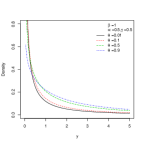
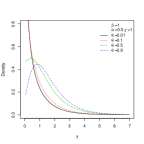
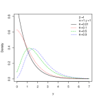
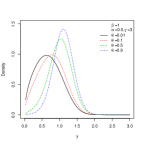
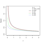
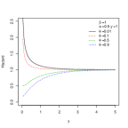
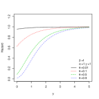
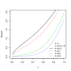
Figure 2: Plots of pdf and hazard rate function of EWB for different values $‎\alpha,‎\beta,‎\gamma‎‎‎$ , $‎\theta‎$ and $m=10$.

From (14), the moment generating function of EWB is

$$\begin{array}[b]{l}M_{Y}(t)=‎\frac{‎\alpha‎‎\theta‎}{(‎\theta+1‎)^{m}-1}‎\sum^{\infty}_{i=0}\sum^{m}_{n=1}\sum^{\infty}_{j=0}‎\frac{(-1)^{j}}{i!}(‎\frac{t}{‎\beta‎}‎)‎^{i}‎\theta‎‎^{n-1}‎{m\choose n}{n\alpha-1\choose j}‎\frac{n‎\Gamma‎\left(1+\frac{i}{\gamma}\right)‎‎}{(j+1)^{1+\frac{i}{\gamma}}}.‎\end{array}$$

$$E(Y^{k})=‎\frac{‎\alpha‎\theta\Gamma‎\left(1+\frac{k}{\gamma}\right)‎‎}{‎\beta‎^{k}‎\left[(‎\theta+1‎)^{m}-1‎\right]‎‎‎‎}‎\sum^{m}_{n=1}\sum^{\infty}_{j=0}(-1)^{j}‎\theta‎‎^{n-1}‎{m\choose n}{n\alpha-1\choose j}‎\frac{n‎‎‎‎}{(j+1)^{1+\frac{k}{\gamma}}}.‎‎$$

14.2 Exponentiated weibull poisson distribution

The exponentiated weibull poisson distribution is a special case of power series distributions with $a_{n}=n!^{-1}$ and $C(‎\theta‎)=‎‎e^{‎\theta‎}-1~{}(‎\theta‎>‎0‎‎)$. Using the cdf in (7), the cdf of exponentiated weibull poisson (EWP) distribution is given by

$$F(y)=‎\frac{e^{‎\theta(1-e^{-(‎\beta y‎)^{‎\gamma‎}})^{‎\alpha‎}}‎-1}{e^{‎\theta‎}-1}‎,$$

$$f(y)=‎\frac{‎\alpha‎\gamma‎\theta‎‎‎‎\beta^{‎\gamma‎}y^{‎\gamma-1‎}‎}{e^{‎\theta‎}-1}e^{-(‎\beta y‎)^{‎\gamma‎}}(1-e^{-(‎\beta y‎)^{‎\gamma‎}})^{‎\alpha-1‎}e^{‎\theta(1-e^{-(‎\beta y‎)^{‎\gamma‎}})^{‎\alpha‎}‎}‎,$$

and

$$h(y)=\frac{‎\alpha‎\gamma‎\theta‎‎‎‎\beta^{‎\gamma‎}y^{‎\gamma-1‎}e^{-(‎\beta y‎)^{‎\gamma‎}}(1-e^{-(‎\beta y)^{‎\gamma‎}})^{‎\alpha-1‎}e^{‎\theta(1-e^{-(‎\beta y)^{‎\gamma‎}})^{‎\alpha‎}‎}}{e^{‎\theta‎}-e^{‎\theta(1-e^{-(‎\beta y‎)^{‎\gamma‎}})^{‎\alpha}}}‎‎.$$

The plots of density and hazard rate function of EWP distribution for some values of $‎\alpha,‎\beta,‎\gamma‎‎‎$ and $‎\theta‎$ are given in Fig. 3.

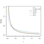
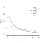
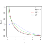
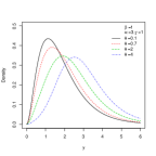
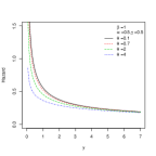
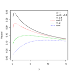
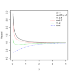
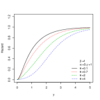
Figure 3: Plots of pdf and hazard rate function of EWP for different values $‎\alpha,‎\beta,‎\gamma‎‎‎$ and $‎\theta‎$.

From (14), the moment generating function of EWP is

$$\begin{array}[b]{l}M_{Y}(t)=\frac{\alpha\theta‎‎}{(e^{\theta}-1)}\sum^{\infty}_{i=0}\sum^{\infty}_{n=1}\sum^{\infty}_{j=0}‎\frac{(-1)^{j}}{i!}‎\frac{\theta^{n-1}}{(n-1)!}(\frac{t}{‎\beta‎})‎^{i}‎{n\alpha-1\choose j}‎\frac{\Gamma(1+\frac{i}{\gamma})}{‎(j+1)^{1+\frac{i}{\gamma}}}.\end{array}$$

$$E(Y^{k})=‎\frac{\alpha\theta‎\Gamma(1+\frac{k}{\gamma})}{\beta^{k}(e^{\theta}-1)}\sum^{\infty}_{n=1}\sum^{\infty}_{j=0}(-1)^{j}{n\alpha-1\choose j}\frac{\theta^{n-1}}{(n-1)!(j+1)^{1+\frac{k}{\gamma}}}.$$

14.3 Exponentiated weibull geometric distribution

The exponentiated weibull geometric distribution is a special case of power series distributions with $a_{n}=1$ and $C(‎\theta‎)=\theta‎‎(1-‎\theta‎)^{-1}~{}(0<‎\theta‎<1)$. Using the cdf in (7), the cdf of exponentiated weibull poisson (EWG) distribution is given by

$$F(y)=\frac{(1-\theta)\left(1-e^{-(\beta y)^{\gamma}}\right)^{\alpha}}{1-\theta\left(1-e^{-(\beta y)^{\gamma}}\right)^{\alpha}}‎,$$

$$f(y)=‎\frac{(1-\theta)\alpha\gamma\beta^{\gamma}y^{\gamma-1}e^{-(\beta y)^{\gamma}}\left(1-e^{-(\beta y)^{\gamma}}\right)^{\alpha-1}}{\left[1-\theta\left(1-e^{-(\beta y)^{\gamma}}\right)^{\alpha}\right]^{2}},$$

and

$$h(y)=\frac{(1-\theta)\alpha\gamma\beta^{\gamma}y^{\gamma-1}e^{-(\beta y)^{\gamma}}\left(1-e^{-(\beta y)^{\gamma}}\right)^{\alpha-1}}{\left[1-\theta\left(1-e^{-(\beta y)^{\gamma}}\right)^{\alpha}\right]\left[1-\left(1-e^{-(\beta y)^{\gamma}}\right)^{\alpha}\right]}.$$

The plots of density and hazard rate function of EWG distribution for some values of $‎\alpha,‎\beta,‎\gamma‎‎‎$ and $‎\theta‎$ are given in Fig. 4.

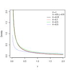
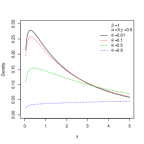
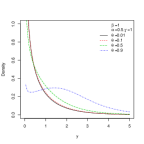
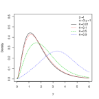
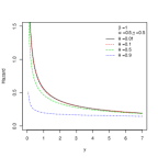
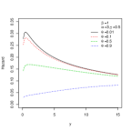
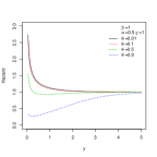
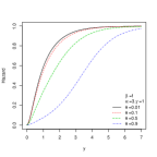
Figure 4: Plots of pdf and hazard rate function of EWG for different values $‎\alpha,‎\beta,‎\gamma‎‎‎$ and $‎\theta‎$.

From (14), the moment generating function of EWP is

$$\begin{array}[b]{l}M_{Y}(t)=\alpha(1-\theta)\sum^{\infty}_{i=0}\sum^{\infty}_{n=1}\sum^{\infty}_{j=0}(-1)^{j}{n\alpha-1\choose j}\Gamma\left(\frac{i}{\gamma}+1\right)\frac{(t/\beta)^{i}}{i!}n\theta^{n-1}(j+1)^{-(\frac{i}{\gamma}+1)}.\end{array}$$

$$E(Y^{k})=(1-\theta)\alpha\beta^{-k}\Gamma\left(\frac{k}{\gamma}+1\right)\sum^{\infty}_{n=1}\sum^{\infty}_{j=0}(-1)^{j}{n\alpha-1\choose j}n\theta^{n-1}(j+1)^{-(\frac{k}{\gamma}+1)}.$$

14.4 Exponentiated weibull logarithmic distribution

The exponentiated weibull logarithmic distribution is a special case of power series distributions with $a_{n}=n^{-1}$ and $C(‎\theta‎)=-‎‎\log‎(1-‎\theta‎)~{}(0<‎\theta‎<1)$. Using the cdf in (7), the cdf of exponentiated weibull poisson (EWL) distribution is given by

$$F(y)=‎‎\frac{\log(1-‎\theta(1-e^{-(\beta y)^{\gamma}})‎^{‎\alpha‎})}{\log(1-‎\theta‎)}‎,$$

$$f(y)=‎\frac{‎\theta‎\alpha\gamma\beta^{\gamma}y^{\gamma-1}e^{-(\beta y)^{\gamma}}\left(1-e^{-(\beta y)^{\gamma}}\right)^{\alpha-1}}{\left[\theta\left(1-e^{-(\beta y)^{\gamma}}\right)^{\alpha}-1\right]\log(1-‎\theta‎)},$$

and

$$h(y)=\frac{‎\theta‎\alpha\gamma\beta^{\gamma}y^{\gamma-1}e^{-(\beta y)^{\gamma}}\left(1-e^{-(\beta y)^{\gamma}}\right)^{\alpha-1}}{\left[\theta\left(1-e^{-(\beta y)^{\gamma}}\right)^{\alpha}-1\right]\log(‎\frac{1-‎\theta‎}{1-‎\theta(1-e^{-(\beta y)^{\gamma}})‎^{‎\alpha‎}}‎)}.$$

The plots of density and hazard rate function of EWL distribution for some values of $‎\alpha,‎\beta,‎\gamma‎‎‎$ and $‎\theta‎$ are given in Fig. 5

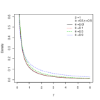
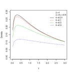
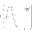
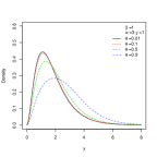
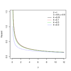
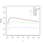
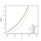
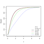
Figure 5: Plots of pdf and hazard rate function of EWL for different values $‎\alpha,‎\beta,‎\gamma‎‎‎$ and $‎\theta‎$.

From (14), the moment generating function of EWL is

$$\begin{array}[b]{l}M_{Y}(t)=‎\frac{‎\alpha‎\theta‎‎}{\log(1-‎\theta‎)}‎\sum^{\infty}_{i=0}\sum^{m}_{n=1}\sum^{\infty}_{j=0}(-1)^{j+1}‎‎\frac{‎\theta‎‎^{n-1}(‎\frac{t}{‎\beta‎}‎)‎^{i}‎}{i!}‎{n\alpha-1\choose j}‎\frac{‎‎\Gamma‎\left(1+\frac{i}{\gamma}\right)‎‎}{(j+1)^{(1+\frac{i}{\gamma})}}.‎\end{array}$$

$$E(Y^{k})=\frac{‎\theta‎\Gamma‎\left(1+\frac{k}{\gamma}\right)‎‎‎}{‎\beta‎^{k}‎‎\log(1-‎\theta‎)}‎\sum^{m}_{n=1}\sum^{\infty}_{j=0}(-1)‎^{j+1}‎{n\alpha-1\choose j}‎\frac{\theta‎‎^{n-1}}{(j+1)^{(1+\frac{k}{\gamma})}}.‎‎$$

15 Applications of the EWPS distribution

In this section we present an application of the EWPS to three real data sets. The fit of EWG, EWP, and EWL on real data sets is examined by graghical methods using MLEs. They are also compared with the EW and Weibull models with respective densities.
The first data set is given by Barreto-Souza(2009), Morais and Cordeiro on the fatigue life (rounded to the nearest thousand cycles) for 67 specimens of Alloy T7987 that failed before having accumulated 300 thousand cycles of testing.
Now, we estimate the parameters of distributions and compare the p-values of Kolmogorov-Smirnov test and AIC (Akaike Information Criterion), AD (Anderson-Darling statistic) and CM (Cram r-von Mises statistic) for these distributions.
The empirical scaled TTT transform (Aarset, [1]) and Kaplan-Meier Curve can be used to identify the shape of the hazard function.
The TTT plot and Kaplan-Meier curve for the first data in Fig. 6 shows an increasing hazard rate function.

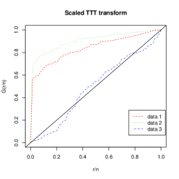
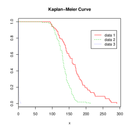
Figure 6: TTT plots and Kaplan-Meier curves of data 1, data 2 and data 3 .

Table 2 lists the MLEs of the parameters, the values of K-S (Kolmogorov-Smirnov) statistic with its respective p-value, -2log(L), AIC (Akaike Information Criterion), AD (Anderson-Darling statistic) and CM (Cram r-von Mises statistic) for the first data. These values show that the EWG, EWL and EW distributions provide a better fit than the EWP and Weibull for fitting the first data.
We apply the Arderson-Darling (AD) and Cram r-von Mises (CM) statistics, in order to verify which distribution fits better to this data. The AD and CM test statistics are described in details in Chen and Balakrishnan [12]. In general, the smaller the values of AD and CM, the better the fit to the data.

Table 2: MLEs(stds.), K-S statistics, p-values, $-2\log(L)$ , AIC, AD and CM for data 1.

Dist.	MLEs	K-S	p-value	$-2\log(L)$	AIC	AD	CM
EWG	$\begin{array}[]{l}\hat{\alpha}=15.3396~{},\hat{\beta}=0.0154\\ \hat{\gamma}=1.3155~{},\hat{\theta}=0.1860\end{array}$	0.0486	0.9974	695.9917	703.9917	0.1968	0.1029
EWP	$\begin{array}[]{l}\hat{\alpha}=20.48~{},\hat{\beta}=0.0732\\ \hat{\gamma}=0.7316~{},\hat{\theta}=13.74\end{array}$	0.0717	0.8811	696.2272	704.2272	0.2205	0.1128
EWL	$\begin{array}[]{l}\hat{\alpha}=14.0601~{},\hat{\beta}=0.0158\\ \hat{\gamma}=1.3671~{},\hat{\theta}=0.7721\end{array}$	0.0524	0.993	696.8654	704.8654	0.2956	0.1165
EW	$\begin{array}[]{l}\hat{\alpha}=12.1645~{},\hat{\beta}=0.0134\\ \hat{‎\gamma‎}=1.4034\end{array}$	0.0522	‎0.9931	696.0166	702.0166	0.19097	0.1023
Weibull	$\hat{\beta}$=0.0054   , $\hat{\gamma}$=3.7349	0.1027	0.4793	706.598	710.598	1.1684	0.2541

As a second application, we consider the data show the fatigue life of 6061-T6 aluminum coupons cut parallel to the direction of rolling and oscillated at 18 cyclers per second. The pooled data, yielding a total of 101 observations, were first analyzed by Birnbaum and Saunders (1969).The TTT plot and Kaplan-Meier curve for this data in Fig. 6 shows an increasing hazard rate function.
The MLEs of the parameters, the values of K-S statistic, p-value, -2log(L), AIC, AD and CM are listed in Table 3. From these values, we note that the EWG model is better than the EWP, EWL, EW and Weibull distributions in terms of fitting to this data.

Table 3: MLEs(stds.), K-S statistics, p-values, $-2\log(L)$ , AIC, AD and CM for data 2.

Dist.	MLEs	K-S	p-value	$-2\log(L)$	AIC	AD	CM
EWG	$\begin{array}[]{l}\hat{\alpha}=8.0516~{},\hat{\beta}=0.0129\\ \hat{\gamma}=2.3695~{},\hat{\theta}=0.7745\end{array}$	0.0618	0.8352	913.1816	921.1816	0.3426	0.1299
EWP	$\begin{array}[]{l}\hat{\alpha}=14.022~{},\hat{\beta}=0.0135\\ \hat{\gamma}=2.1176~{},\hat{\theta}=1.059\end{array}$	0.0791	0.552	913.4216	921.4216	0.4363	0.1557
EWL	$\begin{array}[]{l}\hat{\alpha}=8.9561~{},\hat{\beta}=0.01143\\ \hat{\gamma}=2.4247~{},\hat{\theta}=0.2769\end{array}$	0.0832	0.4867	913.7988	921.7988	0.5413	0.1729
EW	$\begin{array}[]{l}\hat{\alpha}=8.072~{},\hat{\beta}=0.0108\\ \hat{‎\gamma‎}=2.5872\end{array}$	0.082	0.5049	913.498	919.498	0.4597	0.1616
Weibull	$\hat{\beta}$=0.0069   , $\hat{\gamma}$=6.0347	0.1234	0.0923	926.9108	930.9108	1.755	0.3657

The last data set consists 101 observations show the stress-rupture life of kevlar 49/epoxy strands which were subjected to constant sustained pressure at the 90 stress level until all had failed. The failure times in hours are shown in Andrews and Herzberg [3] and Barlow et al. [4]. The TTT plot and Kaplan-Meier curve for this data in Fig. 6 shows bathtub-shaped hazard rate function. The MLEs of the parameters, the values of K-S statistic, p-value, -2log(L), AIC, AD and CM are listed in Table 4. From these values, we note that the EWG and EWP models are better than the EW and Weibull distributions in terms of fitting to this data.

Table 4: MLEs(stds.), K-S statistics, p-values, $-2\log(L)$ , AIC, AD and CM for data 3.

Dist.	MLEs	K-S	p-value	$-2\log(L)$	AIC	AD	CM
EWG	$\begin{array}[]{l}\hat{\alpha}=1.0921~{},\hat{\beta}=3.1202\\ \hat{\gamma}=0.661~{},\hat{\theta}=0.7559\end{array}$	0.0724	0.6657	203.66	211.66	0.7842	0.2019
EWP	$\begin{array}[]{l}\hat{\alpha}=0.8589~{},\hat{\beta}=1.3032\\ \hat{\gamma}=0.8717~{},\hat{\theta}=1.2661\end{array}$	0.0725	0.6638	204.6174	212.6174	0.8409	0.2182
EWL	$\begin{array}[]{l}\hat{\alpha}=2.4513~{},\hat{\beta}=17.0129\\ \hat{\gamma}=0.4978~{},\hat{\theta}=0.9918\end{array}$	0.0898	0.3893	202.4622	210.4622	0.8643	0.2455
EW	$\begin{array}[]{l}\hat{\alpha}=0.7929~{},\hat{\beta}=0.8210\\ \hat{‎\gamma‎}=1.0604\end{array}$	0.0844	0.468	205.5743	211.5743	0.9554	0.2473
Weibull	$\hat{\beta}$=1.0101   , $\hat{\gamma}$=0.9259	0.0906	0.3778	205.9536	209.9536	1.1221	0.2789

Plots of the densities and cumulative distribution functions of the EWG, EWP, EWL, EW and Weibull models fitted to the data sets corresponding to Tables 2, 3 and 4, respectively, are given in Fig. 7, 8 and 9.

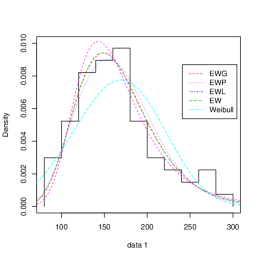
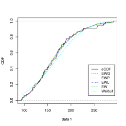
Figure 7: Fitted cdf and survival function of the EWG, EWP, EWL, EW and Weibull distributions for the data sets corresponding to Table 2.

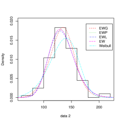
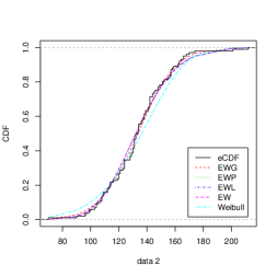
Figure 8: Fitted cdf and survival function of the EWG, EWP, EWL, EW and Weibull distributions for the data sets corresponding to Table 3.

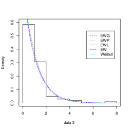
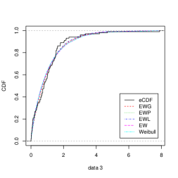
Figure 9: Fitted cdf and survival function of the EWG, EWP, EWL, EW and Weibull distributions for the data sets corresponding to Table 4.

16 Conclusion

Appendix

The elements of the $4\times 4$ observed information matrix $I_{n}\left(\Theta\right)$ are given by

$$\begin{array}[]{ll}I_{\alpha\alpha}&=‎-\frac{n}{‎\alpha‎^{2}‎‎}+‎\sum^{n}_{i=1}‎\frac{‎\theta‎(\log(1-e^{-(‎\beta y‎_{i}‎‎)‎^{‎\gamma‎}‎}))‎^{2}(1-e^{-(‎\beta y‎_{i}‎‎)‎^{‎\gamma‎}‎})‎^{‎\alpha‎}C‎^{\prime‎‎\prime‎}‎(‎\theta(1-e^{-(‎\beta y‎_{i}‎‎)‎^{‎\gamma‎}‎})‎^{‎\alpha‎}‎)‎‎}{C‎^{‎\prime}(‎\theta(1-e^{-(‎\beta y‎_{i}‎‎)‎^{‎\gamma‎}}‎)‎^{‎\alpha‎}‎)‎‎}\vskip 6.0pt plus 2.0pt minus 2.0pt\\ &+\sum^{n}_{i=1}‎‎\frac{‎\theta‎^{2}‎\left[‎(1-e^{-(‎\beta y‎_{i}‎‎)‎^{‎\gamma‎}‎})‎^{‎\alpha‎}‎\log(1-e^{-(‎\beta y‎_{i}‎‎)‎^{‎\gamma‎}‎})\right]‎^{2}C‎^{\prime\prime\prime}(‎\theta(1-e^{-(‎\beta y‎_{i}‎‎)‎^{‎\gamma‎}‎})‎^{‎\alpha‎})‎‎‎}{C‎^{‎\prime}(‎\theta(1-e^{-(‎\beta y‎_{i}‎‎)‎^{‎\gamma‎}}‎)‎^{‎\alpha‎}‎)}\vskip 6.0pt plus 2.0pt minus 2.0pt\\ &-\sum^{n}_{i=1}‎\frac{\theta‎^{2}((1-e^{-(‎\beta y‎_{i}‎‎)‎^{‎\gamma‎}‎})‎^{‎\alpha‎})‎^{2}‎(\log(1-e^{-(‎\beta y‎_{i}‎‎)‎^{‎\gamma‎}‎}))‎^{2}(C‎^{\prime‎‎\prime‎}‎(‎\theta(1-e^{-(‎\beta y‎_{i}‎‎)‎^{‎\gamma‎}‎})‎^{‎\alpha‎}‎)‎‎)^{2}‎}{(C‎^{‎\prime}(‎\theta(1-e^{-(‎\beta y‎_{i}‎‎)‎^{‎\gamma‎}}‎)‎^{‎\alpha‎}‎))^{2}}‎‎‎,\vskip 12.0pt plus 4.0pt minus 4.0pt\\ \\ I_{\alpha\beta}&=\sum^{n}_{i=1}‎‎\frac{‎\gamma‎\beta‎^{‎\gamma‎-1}‎‎‎y‎_{i}‎‎^{‎\gamma‎}e^{-(‎\beta y‎_{i}‎‎)‎^{‎\gamma‎}‎}‎}{1-e^{-(‎\beta y‎_{i}‎‎)‎^{‎\gamma‎}‎}}‎\vskip 6.0pt plus 2.0pt minus 2.0pt\\ &+‎\sum^{n}_{i=1}\frac{‎\theta\gamma‎\beta‎^{‎\gamma‎-1}‎‎‎y‎_{i}‎‎^{‎\gamma‎}e^{-(‎\beta y‎_{i}‎‎)‎^{‎\gamma‎}‎}‎(1-e^{-(‎\beta y‎_{i}‎‎)‎^{‎\gamma‎}‎})‎^{‎\alpha-1‎}C‎^{\prime‎‎\prime‎}‎(‎\theta(1-e^{-(‎\beta y‎_{i}‎‎)‎^{‎\gamma‎}‎})‎^{‎\alpha‎}‎)‎‎‎}{C‎^{‎\prime}(‎\theta(1-e^{-(‎\beta y‎_{i}‎‎)‎^{‎\gamma‎}}‎)‎^{‎\alpha‎}‎)‎‎}‎\vskip 6.0pt plus 2.0pt minus 2.0pt\\ &+\sum^{n}_{i=1}‎\frac{‎\theta‎\alpha‎\gamma‎\beta‎^{‎\gamma‎-1}‎‎‎y‎_{i}‎‎^{‎\gamma‎}e^{-(‎\beta y‎_{i}‎‎)‎^{‎\gamma‎}‎}‎‎‎\log(1-e^{-(‎\beta y‎_{i}‎‎)‎^{‎\gamma‎}‎})‎(1-e^{-(‎\beta y‎_{i}‎‎)‎^{‎\gamma‎}‎})‎^{‎\alpha-1‎}C‎^{\prime‎‎\prime‎}‎(‎\theta(1-e^{-(‎\beta y‎_{i}‎‎)‎^{‎\gamma‎}‎})‎^{‎\alpha‎}‎)}{C‎^{‎\prime}(‎\theta(1-e^{-(‎\beta y‎_{i}‎‎)‎^{‎\gamma‎}}‎)‎^{‎\alpha‎}‎)‎‎}‎‎\vskip 6.0pt plus 2.0pt minus 2.0pt\\ &+\sum^{n}_{i=1}‎\frac{\theta‎^{2}‎‎\alpha‎\gamma‎\beta‎^{‎\gamma‎-1}‎‎‎y‎_{i}‎‎^{‎\gamma‎}e^{-(‎\beta y‎_{i}‎‎)‎^{‎\gamma‎}‎}‎‎‎\log(1-e^{-(‎\beta y‎_{i}‎‎)‎^{‎\gamma‎}‎})‎(1-e^{-(‎\beta y‎_{i}‎‎)‎^{‎\gamma‎}‎})‎^{‎2\alpha-1‎}C‎^{\prime‎‎\prime‎\prime‎}‎(‎\theta(1-e^{-(‎\beta y‎_{i}‎‎)‎^{‎\gamma‎}‎})‎^{‎\alpha‎}‎)}{C‎^{‎\prime}(‎\theta(1-e^{-(‎\beta y‎_{i}‎‎)‎^{‎\gamma‎}}‎)‎^{‎\alpha‎}‎)‎‎}‎‎\vskip 6.0pt plus 2.0pt minus 2.0pt\\ &-\sum^{n}_{i=1}‎\frac{\theta‎^{2}‎‎\alpha‎\gamma‎\beta‎^{‎\gamma‎-1}‎‎‎y‎_{i}‎‎^{‎\gamma‎}e^{-(‎\beta y‎_{i}‎‎)‎^{‎\gamma‎}‎}‎‎‎\log(1-e^{-(‎\beta y‎_{i}‎‎)‎^{‎\gamma‎}‎})‎(1-e^{-(‎\beta y‎_{i}‎‎)‎^{‎\gamma‎}‎})‎^{‎2\alpha-1‎}(C‎^{\prime‎‎\prime}‎(‎\theta(1-e^{-(‎\beta y‎_{i}‎‎)‎^{‎\gamma‎}‎})‎^{‎\alpha‎}‎))‎^{2}‎}{(C‎^{‎\prime}(‎\theta(1-e^{-(‎\beta y‎_{i}‎‎)‎^{‎\gamma‎}}‎)‎^{‎\alpha‎}‎))^{2}‎‎}‎‎‎,\vskip 12.0pt plus 4.0pt minus 4.0pt\\ \\ I_{\alpha‎\gamma‎}&=\sum^{n}_{i=1}‎\frac{‎\beta‎^{‎\gamma‎}‎‎‎y‎_{i}‎‎^{‎\gamma‎}\log(‎\beta‎‎‎y‎_{i}‎)e^{-(‎\beta y‎_{i}‎‎)‎^{‎\gamma‎}‎}‎‎‎}{1-e^{-(‎\beta y‎_{i}‎‎)‎^{‎\gamma‎}‎}}‎\vskip 6.0pt plus 2.0pt minus 2.0pt\\ &+\sum^{n}_{i=1}‎\frac{‎\theta‎\beta‎^{‎\gamma‎}‎‎‎y‎_{i}‎‎^{‎\gamma‎}\log(‎\beta‎‎‎y‎_{i}‎)e^{-(‎\beta y‎_{i}‎‎)‎^{‎\gamma‎}‎}‎(1-e^{-(‎\beta y‎_{i}‎‎)‎^{‎\gamma‎}‎})‎^{‎\alpha-1‎}C‎^{\prime‎‎\prime‎}‎(‎\theta(1-e^{-(‎\beta y‎_{i}‎‎)‎^{‎\gamma‎}‎})‎^{‎\alpha‎}‎)‎‎‎}{C‎^{‎\prime}(‎\theta(1-e^{-(‎\beta y‎_{i}‎‎)‎^{‎\gamma‎}}‎)‎^{‎\alpha‎}‎)‎‎}\vskip 6.0pt plus 2.0pt minus 2.0pt\\ &+\sum^{n}_{i=1}‎‎\frac{‎\theta‎‎\alpha‎‎\beta‎^{‎\gamma‎}‎‎‎y‎_{i}‎‎^{‎\gamma‎}\log(‎\beta‎‎‎y‎_{i}‎)e^{-(‎\beta y‎_{i}‎‎)‎^{‎\gamma‎}‎}\log(1-e^{-(‎\beta y‎_{i}‎‎)‎^{‎\gamma‎}‎})‎(1-e^{-(‎\beta y‎_{i}‎‎)‎^{‎\gamma‎}‎})‎^{‎\alpha-1‎}C‎^{\prime‎‎\prime‎}‎(‎\theta(1-e^{-(‎\beta y‎_{i}‎‎)‎^{‎\gamma‎}‎})‎^{‎\alpha‎}‎)}{C‎^{‎\prime}(‎\theta(1-e^{-(‎\beta y‎_{i}‎‎)‎^{‎\gamma‎}}‎)‎^{‎\alpha‎}‎)}‎\vskip 6.0pt plus 2.0pt minus 2.0pt\\ &+\sum^{n}_{i=1}‎\frac{\theta‎^{2}‎\alpha‎‎\beta‎^{‎\gamma‎}‎‎‎y‎_{i}‎‎^{‎\gamma‎}\log(‎\beta‎‎‎y‎_{i}‎)e^{-(‎\beta y‎_{i}‎‎)‎^{‎\gamma‎}‎}\log(1-e^{-(‎\beta y‎_{i}‎‎)‎^{‎\gamma‎}‎})‎(1-e^{-(‎\beta y‎_{i}‎‎)‎^{‎\gamma‎}‎})‎^{‎2\alpha-1‎}C‎^{\prime‎‎\prime\prime‎‎}‎(‎\theta(1-e^{-(‎\beta y‎_{i}‎‎)‎^{‎\gamma‎}‎})‎^{‎\alpha‎}‎)}{C‎^{‎\prime}(‎\theta(1-e^{-(‎\beta y‎_{i}‎‎)‎^{‎\gamma‎}}‎)‎^{‎\alpha‎}‎)}‎‎\vskip 6.0pt plus 2.0pt minus 2.0pt\\ &-\sum^{n}_{i=1}‎‎\frac{\theta‎^{2}‎\alpha‎‎\beta‎^{‎\gamma‎}‎‎‎y‎_{i}‎‎^{‎\gamma‎}\log(‎\beta‎‎‎y‎_{i}‎)e^{-(‎\beta y‎_{i}‎‎)‎^{‎\gamma‎}‎}\log(1-e^{-(‎\beta y‎_{i}‎‎)‎^{‎\gamma‎}‎})‎(1-e^{-(‎\beta y‎_{i}‎‎)‎^{‎\gamma‎}‎})‎^{‎2\alpha-1‎}(C‎^{\prime‎‎\prime‎‎}‎(‎\theta(1-e^{-(‎\beta y‎_{i}‎‎)‎^{‎\gamma‎}‎})‎^{‎\alpha‎}‎))^{2}}{(C‎^{‎\prime}(‎\theta(1-e^{-(‎\beta y‎_{i}‎‎)‎^{‎\gamma‎}}‎)‎^{‎\alpha‎}‎))^{2}}‎‎‎‎,\vskip 12.0pt plus 4.0pt minus 4.0pt\\ \\ I_{\alpha‎‎\theta‎‎}&=\sum^{n}_{i=1}‎\frac{\log(1-e^{-(‎\beta y‎_{i}‎‎)‎^{‎\gamma‎}‎})(1-e^{-(‎\beta y‎_{i}‎‎)‎^{‎\gamma‎}}‎)‎^{‎\alpha‎}C‎^{\prime‎‎\prime‎}‎(‎\theta(1-e^{-(‎\beta y‎_{i}‎‎)‎^{‎\gamma‎}‎})‎^{‎\alpha‎}‎)}{C‎^{‎\prime}(‎\theta(1-e^{-(‎\beta y‎_{i}‎‎)‎^{‎\gamma‎}}‎)‎^{‎\alpha‎}‎)}‎\vskip 6.0pt plus 2.0pt minus 2.0pt\\ &+\sum^{n}_{i=1}‎\frac{‎\theta\log(1-e^{-(‎\beta y‎_{i}‎‎)‎^{‎\gamma‎}‎})‎‎(1-e^{-(‎\beta y‎_{i}‎‎)‎^{‎\gamma‎}‎})‎^{‎2\alpha‎}C‎^{\prime‎‎\prime\prime‎}‎(‎\theta(1-e^{-(‎\beta y‎_{i}‎‎)‎^{‎\gamma‎}‎})‎^{‎\alpha‎}‎)}{C‎^{‎\prime}(‎\theta(1-e^{-(‎\beta y‎_{i}‎‎)‎^{‎\gamma‎}}‎)‎^{‎\alpha‎}‎)}\vskip 6.0pt plus 2.0pt minus 2.0pt\\ &-\sum^{n}_{i=1}‎‎\frac{‎\theta\log(1-e^{-(‎\beta y‎_{i}‎‎)‎^{‎\gamma‎}‎})‎‎(1-e^{-(‎\beta y‎_{i}‎‎)‎^{‎\gamma‎}‎})‎^{‎2\alpha‎}(C‎^{\prime‎‎\prime‎}‎(‎\theta(1-e^{-(‎\beta y‎_{i}‎‎)‎^{‎\gamma‎}‎})‎^{‎\alpha‎}‎))^{2}}{(C‎^{‎\prime}(‎\theta(1-e^{-(‎\beta y‎_{i}‎‎)‎^{‎\gamma‎}}‎)‎^{‎\alpha‎}‎))^{2}},\vskip 12.0pt plus 4.0pt minus 4.0pt\\ ‎\end{array}$$

$$\begin{array}[]{ll}I_{‎\beta‎\beta‎‎‎‎}&=-‎\frac{n‎\gamma‎}{‎\beta^{2}‎}‎-\sum^{n}_{i=1}‎\gamma‎(‎\gamma-1‎)\beta‎^{‎\gamma‎-2}y‎_{i}‎‎^{‎\gamma‎}+\sum^{n}_{i=1}‎\frac{(‎\alpha-1‎)‎\gamma(‎\gamma-1‎)‎\beta‎^{‎\gamma‎-2}e^{-(‎\beta y‎_{i}‎‎)^{‎\gamma‎}‎}}{1-e^{-(‎\beta y‎_{i}‎‎)‎^{‎\gamma‎}}‎}‎‎\vskip 6.0pt plus 2.0pt minus 2.0pt\\ &-\sum^{n}_{i=1}‎\frac{‎(‎\alpha-1‎)‎\gamma^{2}\beta‎^{2‎\gamma‎-2}‎y‎_{i}‎‎^{2‎\gamma‎}e^{-(‎\beta y‎_{i}‎‎)‎^{‎\gamma‎}}‎}{1-e^{-(‎\beta y‎_{i}‎‎)‎^{‎\gamma‎}}}-\sum^{n}_{i=1}‎\frac{\gamma^{2}\beta‎^{2‎\gamma‎-2}‎y‎_{i}‎‎^{2‎\gamma‎}(e^{-(‎\beta y‎_{i}‎‎)‎^{‎\gamma‎}})^{2}‎}{(1-e^{-(‎\beta y‎_{i}‎‎)‎^{‎\gamma‎}})^{2}}‎‎‎\vskip 6.0pt plus 2.0pt minus 2.0pt\\ &+\sum^{n}_{i=1}‎\frac{‎\theta‎‎\alpha‎\gamma(‎\gamma-1‎)‎‎y‎_{i}‎‎^{‎\gamma‎}\beta‎^{‎\gamma‎-2}e^{-(‎\beta y‎_{i}‎‎)‎^{‎\gamma‎}}(1-e^{-(‎\beta y‎_{i}‎‎)‎^{‎\gamma‎}}‎)‎^{‎\alpha-1‎}C‎^{\prime‎‎\prime‎}‎(‎\theta(1-e^{-(‎\beta y‎_{i}‎‎)‎^{‎\gamma‎}‎})‎^{‎\alpha‎}‎)}{C‎^{‎\prime}(‎\theta(1-e^{-(‎\beta y‎_{i}‎‎)‎^{‎\gamma‎}}‎)‎^{‎\alpha‎}‎)}‎‎‎\vskip 6.0pt plus 2.0pt minus 2.0pt\\ &-\sum^{n}_{i=1}‎\frac{‎\theta‎‎\alpha‎\gamma^{2}‎‎y‎_{i}‎‎^{‎2\gamma‎}\beta‎^{2‎\gamma‎-2}e^{-(‎\beta y‎_{i}‎‎)‎^{‎\gamma‎}}(1-e^{-(‎\beta y‎_{i}‎‎)‎^{‎\gamma‎}}‎)‎^{‎\alpha-1‎}C‎^{\prime‎‎\prime‎}‎(‎\theta(1-e^{-(‎\beta y‎_{i}‎‎)‎^{‎\gamma‎}‎})‎^{‎\alpha‎})}{C‎^{‎\prime}(‎\theta(1-e^{-(‎\beta y‎_{i}‎‎)‎^{‎\gamma‎}}‎)‎^{‎\alpha‎}‎)}‎‎‎‎\vskip 6.0pt plus 2.0pt minus 2.0pt\\ &+\sum^{n}_{i=1}‎\frac{(‎‎\alpha‎-1‎)\theta‎‎\alpha‎\gamma^{2}‎‎y‎_{i}‎‎^{‎2\gamma‎}\beta‎^{2‎\gamma‎-2}(e^{-(‎\beta y‎_{i}‎‎)‎^{‎\gamma‎}})^{2}(1-e^{-(‎\beta y‎_{i}‎‎)‎^{‎\gamma‎}}‎)‎^{‎\alpha-2‎}C‎^{\prime‎‎\prime‎}‎(‎\theta(1-e^{-(‎\beta y‎_{i}‎‎)‎^{‎\gamma‎}‎})‎^{‎\alpha‎}‎)}{C‎^{‎\prime}(‎\theta(1-e^{-(‎\beta y‎_{i}‎‎)‎^{‎\gamma‎}}‎)‎^{‎\alpha‎}‎)}‎‎‎‎\vskip 6.0pt plus 2.0pt minus 2.0pt\\ &+\sum^{n}_{i=1}‎\frac{\theta‎‎^{2}‎‎\alpha‎^{2}‎‎\gamma^{2}‎‎y‎_{i}‎‎^{‎2\gamma‎}\beta‎^{2‎\gamma‎-2}(e^{-(‎\beta y‎_{i}‎‎)‎^{‎\gamma‎}})^{2}(1-e^{-(‎\beta y‎_{i}‎‎)‎^{‎\gamma‎}}‎)‎^{‎2\alpha-2‎}C‎^{\prime‎‎\prime\prime‎}‎(‎\theta(1-e^{-(‎\beta y‎_{i}‎‎)‎^{‎\gamma‎}‎})‎^{‎\alpha‎}‎)}{C‎^{‎\prime}(‎\theta(1-e^{-(‎\beta y‎_{i}‎‎)‎^{‎\gamma‎}}‎)‎^{‎\alpha‎}‎)}‎‎‎‎\vskip 6.0pt plus 2.0pt minus 2.0pt\\ &-\sum^{n}_{i=1}‎\frac{\theta‎‎^{2}‎‎\alpha‎^{2}‎‎\gamma^{2}‎‎y‎_{i}‎‎^{‎2\gamma‎}\beta‎^{2‎\gamma‎-2}(e^{-(‎\beta y‎_{i}‎‎)‎^{‎\gamma‎}})^{2}(1-e^{-(‎\beta y‎_{i}‎‎)‎^{‎\gamma‎}}‎)‎^{‎2\alpha-2‎}(C‎^{\prime‎‎\prime‎}‎(‎\theta(1-e^{-(‎\beta y‎_{i}‎‎)‎^{‎\gamma‎}‎})‎^{‎\alpha‎}‎))‎^{2}‎}{(C‎^{‎\prime}(‎\theta(1-e^{-(‎\beta y‎_{i}‎‎)‎^{‎\gamma‎}}‎)‎^{‎\alpha‎}‎))‎^{2}‎},\vskip 12.0pt plus 4.0pt minus 4.0pt\\ \\ I_{‎\beta‎‎\gamma‎‎‎‎‎}&=‎\frac{1}{‎\beta‎}‎-\sum^{n}_{i=1}‎\gamma‎\beta‎^{‎\gamma‎-1}y‎_{i}‎‎^{‎\gamma‎}‎\log‎(‎\beta y‎_{i}‎)-\sum^{n}_{i=1}‎‎\beta‎^{‎\gamma‎-1}y‎_{i}‎‎^{‎\gamma‎}\vskip 6.0pt plus 2.0pt minus 2.0pt\\ &+\sum^{n}_{i=1}‎\frac{‎\gamma(‎\alpha-1‎)‎\beta‎^{‎\gamma‎-1}‎‎‎y‎_{i}‎‎^{‎\gamma‎}\log(‎\beta‎‎‎y‎_{i}‎)e^{-(‎\beta y‎_{i}‎‎)‎^{‎\gamma‎}‎}‎‎‎}{1-e^{-(‎\beta y‎_{i}‎‎)‎^{‎\gamma‎}‎}}‎+\sum^{n}_{i=1}‎‎‎\frac{(‎\alpha-1‎)‎\beta‎^{‎\gamma‎-1}‎‎‎y‎_{i}‎‎^{‎\gamma‎}e^{-(‎\beta y‎_{i}‎‎)‎^{‎\gamma‎}‎}‎‎‎}{1-e^{-(‎\beta y‎_{i}‎‎)‎^{‎\gamma‎}‎}}\vskip 6.0pt plus 2.0pt minus 2.0pt\\ &-\sum^{n}_{i=1}‎‎\frac{(‎\alpha-1‎)‎\gamma‎‎\beta‎^{2‎\gamma‎-1}‎‎‎y‎_{i}‎‎^{‎2\gamma‎}\log‎(‎\beta y‎_{i}‎)e^{-(‎\beta y‎_{i}‎‎)‎^{‎\gamma‎}‎}‎‎‎}{1-e^{-(‎\beta y‎_{i}‎‎)‎^{‎\gamma‎}‎}}‎-\sum^{n}_{i=1}‎\frac{(‎\alpha-1‎)‎\gamma‎‎\beta‎^{2‎\gamma‎-1}‎‎‎y‎_{i}‎‎^{‎2\gamma‎}\log‎(‎\beta y‎_{i}‎)(e^{-(‎\beta y‎_{i}‎‎)‎^{‎\gamma‎}‎}‎‎‎)^{2}}{(1-e^{-(‎\beta y‎_{i}‎‎)‎^{‎\gamma‎}‎})^{2}}‎\vskip 6.0pt plus 2.0pt minus 2.0pt\\ &+\sum^{n}_{i=1}‎‎\frac{‎\theta‎‎\alpha‎\gamma‎‎y‎_{i}‎‎^{‎\gamma‎}\beta‎^{‎\gamma‎-1}\log‎(‎\beta y‎_{i}‎)e^{-(‎\beta y‎_{i}‎‎)‎^{‎\gamma‎}}(1-e^{-(‎\beta y‎_{i}‎‎)‎^{‎\gamma‎}}‎)‎^{‎\alpha-1‎}C‎^{\prime‎‎\prime‎}‎(‎\theta(1-e^{-(‎\beta y‎_{i}‎‎)‎^{‎\gamma‎}‎})‎^{‎\alpha‎}‎)}{C‎^{‎\prime}(‎\theta(1-e^{-(‎\beta y‎_{i}‎‎)‎^{‎\gamma‎}}‎)‎^{‎\alpha‎}‎)}‎‎‎\vskip 6.0pt plus 2.0pt minus 2.0pt\\ &+\sum^{n}_{i=1}‎‎‎\frac{‎\theta‎‎\alpha‎‎‎y‎_{i}‎‎^{‎\gamma‎}\beta‎^{‎\gamma‎-1}e^{-(‎\beta y‎_{i}‎‎)‎^{‎\gamma‎}}(1-e^{-(‎\beta y‎_{i}‎‎)‎^{‎\gamma‎}}‎)‎^{‎\alpha-1‎}C‎^{\prime‎‎\prime‎}‎(‎\theta(1-e^{-(‎\beta y‎_{i}‎‎)‎^{‎\gamma‎}‎})‎^{‎\alpha‎}‎)}{C‎^{‎\prime}(‎\theta(1-e^{-(‎\beta y‎_{i}‎‎)‎^{‎\gamma‎}}‎)‎^{‎\alpha‎}‎)}‎‎‎\vskip 6.0pt plus 2.0pt minus 2.0pt\\ &-\sum^{n}_{i=1}‎‎‎\frac{‎\theta‎‎\alpha‎\gamma‎‎y‎_{i}‎‎^{‎2\gamma‎}\beta‎^{‎2\gamma‎-1}\log‎(‎\beta y‎_{i}‎)e^{-(‎\beta y‎_{i}‎‎)‎^{‎\gamma‎}}(1-e^{-(‎\beta y‎_{i}‎‎)‎^{‎\gamma‎}}‎)‎^{‎\alpha-1‎}C‎^{\prime‎‎\prime‎}‎(‎\theta(1-e^{-(‎\beta y‎_{i}‎‎)‎^{‎\gamma‎}‎})‎^{‎\alpha‎}‎)}{C‎^{‎\prime}(‎\theta(1-e^{-(‎\beta y‎_{i}‎‎)‎^{‎\gamma‎}}‎)‎^{‎\alpha‎}‎)}‎‎‎\vskip 6.0pt plus 2.0pt minus 2.0pt\\ &+\sum^{n}_{i=1}‎‎‎‎‎‎\frac{‎(‎\alpha-1‎)\theta‎‎\alpha‎\gamma‎‎y‎_{i}‎‎^{‎2\gamma‎}\beta‎^{‎2\gamma‎-1}\log‎(‎\beta y‎_{i}‎)(e^{-(‎\beta y‎_{i}‎‎)‎^{‎\gamma‎}})^{2}(1-e^{-(‎\beta y‎_{i}‎‎)‎^{‎\gamma‎}}‎)‎^{‎\alpha-2‎}C‎^{\prime‎‎\prime‎}‎(‎\theta(1-e^{-(‎\beta y‎_{i}‎‎)‎^{‎\gamma‎}‎})‎^{‎\alpha‎}‎)}{C‎^{‎\prime}(‎\theta(1-e^{-(‎\beta y‎_{i}‎‎)‎^{‎\gamma‎}}‎)‎^{‎\alpha‎}‎)}‎‎‎\vskip 6.0pt plus 2.0pt minus 2.0pt\\ &+\sum^{n}_{i=1}‎‎‎‎‎‎‎‎‎\frac{‎\theta‎^{2}‎\alpha^{2}‎\gamma‎‎y‎_{i}‎‎^{‎2\gamma‎}\beta‎^{‎2\gamma‎-1}\log‎(‎\beta y‎_{i}‎)(e^{-(‎\beta y‎_{i}‎‎)‎^{‎\gamma‎}})^{2}(1-e^{-(‎\beta y‎_{i}‎‎)‎^{‎\gamma‎}}‎)‎^{‎2\alpha-2‎}C‎^{\prime‎‎\prime\prime‎}‎(‎\theta(1-e^{-(‎\beta y‎_{i}‎‎)‎^{‎\gamma‎}‎})‎^{‎\alpha‎}‎)}{C‎^{‎\prime}(‎\theta(1-e^{-(‎\beta y‎_{i}‎‎)‎^{‎\gamma‎}}‎)‎^{‎\alpha‎}‎)}‎‎‎\vskip 6.0pt plus 2.0pt minus 2.0pt\\ &-\sum^{n}_{i=1}‎‎‎\frac{‎\theta‎^{2}‎\alpha^{2}‎\gamma‎‎y‎_{i}‎‎^{‎2\gamma‎}\beta‎^{‎2\gamma‎-1}\log‎(‎\beta y‎_{i}‎)(e^{-(‎\beta y‎_{i}‎‎)‎^{‎\gamma‎}})^{2}(1-e^{-(‎\beta y‎_{i}‎‎)‎^{‎\gamma‎}}‎)‎^{‎2\alpha-2‎}(C‎^{\prime‎‎\prime‎}‎(‎\theta(1-e^{-(‎\beta y‎_{i}‎‎)‎^{‎\gamma‎}‎})‎^{‎\alpha‎}‎))^{2}}{(C‎^{‎\prime}(‎\theta(1-e^{-(‎\beta y‎_{i}‎‎)‎^{‎\gamma‎}}‎)‎^{‎\alpha‎}‎))^{2}},\vskip 12.0pt plus 4.0pt minus 4.0pt\\ \\ I_{‎\beta‎\theta‎‎‎‎‎‎}&=\sum^{n}_{i=1}‎‎‎‎‎‎‎‎‎‎‎\frac{‎‎\alpha‎\gamma‎‎y‎_{i}‎‎^{‎\gamma‎}\beta‎^{‎\gamma‎-1}e^{-(‎\beta y‎_{i}‎‎)‎^{‎\gamma‎}}(1-e^{-(‎\beta y‎_{i}‎‎)‎^{‎\gamma‎}}‎)‎^{‎\alpha-1‎}C‎^{\prime‎‎\prime‎}‎(‎\theta(1-e^{-(‎\beta y‎_{i}‎‎)‎^{‎\gamma‎}‎})‎^{‎\alpha‎}‎)}{C‎^{‎\prime}(‎\theta(1-e^{-(‎\beta y‎_{i}‎‎)‎^{‎\gamma‎}}‎)‎^{‎\alpha‎}‎)}‎‎‎\vskip 6.0pt plus 2.0pt minus 2.0pt\\ &+\sum^{n}_{i=1}‎‎‎‎‎\frac{‎\theta‎‎\alpha‎\gamma‎‎y‎_{i}‎‎^{‎\gamma‎}\beta‎^{‎\gamma‎-1}e^{-(‎\beta y‎_{i}‎‎)‎^{‎\gamma‎}}(1-e^{-(‎\beta y‎_{i}‎‎)‎^{‎\gamma‎}}‎)‎^{2‎\alpha-1‎}C‎^{\prime‎‎\prime\prime‎}‎(‎\theta(1-e^{-(‎\beta y‎_{i}‎‎)‎^{‎\gamma‎}‎})‎^{‎\alpha‎}‎)}{C‎^{‎\prime}(‎\theta(1-e^{-(‎\beta y‎_{i}‎‎)‎^{‎\gamma‎}}‎)‎^{‎\alpha‎}‎)}‎‎‎\vskip 6.0pt plus 2.0pt minus 2.0pt\\ &-\sum^{n}_{i=1}\frac{‎\theta‎‎\alpha‎\gamma‎‎y‎_{i}‎‎^{‎\gamma‎}\beta‎^{‎\gamma‎-1}e^{-(‎\beta y‎_{i}‎‎)‎^{‎\gamma‎}}(1-e^{-(‎\beta y‎_{i}‎‎)‎^{‎\gamma‎}}‎)‎^{2‎\alpha-1‎}(C‎^{\prime‎‎\prime}‎(‎\theta(1-e^{-(‎\beta y‎_{i}‎‎)‎^{‎\gamma‎}‎})‎^{‎\alpha‎}‎))^{2}}{(C‎^{‎\prime}(‎\theta(1-e^{-(‎\beta y‎_{i}‎‎)‎^{‎\gamma‎}}‎)‎^{‎\alpha‎}‎))^{2}},\vskip 12.0pt plus 4.0pt minus 4.0pt\\ \\ \end{array}$$

$$\begin{array}[]{ll}I_{‎‎\gamma‎\gamma‎‎‎‎‎‎‎‎}&=-‎\frac{n}{‎\gamma^{2}‎}‎-\sum^{n}_{i=1}‎\beta‎^{‎\gamma‎}y‎_{i}‎‎^{‎\gamma‎}(‎\log‎(‎\beta y‎_{i}‎))^{2}+\sum^{n}_{i=1}‎\frac{‎(‎\alpha-1‎)\beta‎^{‎\gamma‎}y‎_{i}‎‎^{‎\gamma‎}(‎\log‎(‎\beta y‎_{i}‎))^{2}e^{-(‎\beta y‎_{i}‎‎)‎^{‎\gamma‎}}}{1-e^{-(‎\beta y‎_{i}‎‎)‎^{‎\gamma‎}‎}}‎‎‎‎\vskip 6.0pt plus 2.0pt minus 2.0pt\\ &-\sum^{n}_{i=1}‎\frac{‎(‎\alpha-1‎)\beta‎^{2‎\gamma‎}y‎_{i}‎‎^{‎2\gamma‎}(‎\log‎(‎\beta y‎_{i}‎))^{2}e^{-(‎\beta y‎_{i}‎‎)‎^{‎\gamma‎}}}{1-e^{-(‎\beta y‎_{i}‎‎)‎^{‎\gamma‎}‎}}-\sum^{n}_{i=1}\frac{‎(‎\alpha-1‎)\beta‎^{2‎\gamma‎}y‎_{i}‎‎^{‎2\gamma‎}(‎\log‎(‎\beta y‎_{i}‎))^{2}e^{-(‎\beta y‎_{i}‎‎)‎^{‎2\gamma‎}}}{(1-e^{-(‎\beta y‎_{i}‎‎)‎^{‎\gamma‎}‎})^{2}}‎‎‎‎\vskip 6.0pt plus 2.0pt minus 2.0pt\\ &+\sum^{n}_{i=1}\frac{‎\theta‎‎\alpha‎‎‎\beta‎^{‎\gamma‎}y‎_{i}‎‎^{‎\gamma‎}(\log‎(‎\beta y‎_{i}‎))^{2}e^{-(‎\beta y‎_{i}‎‎)‎^{‎\gamma‎}}(1-e^{-(‎\beta y‎_{i}‎‎)‎^{‎\gamma‎}}‎)‎^{‎\alpha-1‎}C‎^{\prime‎‎\prime‎}‎(‎\theta(1-e^{-(‎\beta y‎_{i}‎‎)‎^{‎\gamma‎}‎})‎^{‎\alpha‎}‎)}{C‎^{‎\prime}(‎\theta(1-e^{-(‎\beta y‎_{i}‎‎)‎^{‎\gamma‎}}‎)‎^{‎\alpha‎}‎)}‎‎‎\vskip 6.0pt plus 2.0pt minus 2.0pt\\ &-\sum^{n}_{i=1}\frac{‎\theta‎‎\alpha‎‎‎\beta‎^{2‎\gamma‎}y‎_{i}‎‎^{‎2\gamma‎}(\log‎(‎\beta y‎_{i}‎))^{2}e^{-(‎\beta y‎_{i}‎‎)‎^{‎\gamma‎}}(1-e^{-(‎\beta y‎_{i}‎‎)‎^{‎\gamma‎}}‎)‎^{‎\alpha-1‎}C‎^{\prime‎‎\prime‎}‎(‎\theta(1-e^{-(‎\beta y‎_{i}‎‎)‎^{‎\gamma‎}‎})‎^{‎\alpha‎}‎)}{C‎^{‎\prime}(‎\theta(1-e^{-(‎\beta y‎_{i}‎‎)‎^{‎\gamma‎}}‎)‎^{‎\alpha‎}‎)}‎‎‎\vskip 6.0pt plus 2.0pt minus 2.0pt\\ &+\sum^{n}_{i=1}\frac{‎\theta‎‎\alpha(‎\alpha-1‎)‎‎‎\beta‎^{2‎\gamma‎}y‎_{i}‎‎^{‎2\gamma‎}(\log‎(‎\beta y‎_{i}‎))^{2}(e^{-(‎\beta y‎_{i}‎‎)‎^{‎\gamma‎}})^{2}(1-e^{-(‎\beta y‎_{i}‎‎)‎^{‎\gamma‎}}‎)‎^{‎\alpha-2‎}C‎^{\prime‎‎\prime‎}‎(‎\theta(1-e^{-(‎\beta y‎_{i}‎‎)‎^{‎\gamma‎}‎})‎^{‎\alpha‎}‎)}{C‎^{‎\prime}(‎\theta(1-e^{-(‎\beta y‎_{i}‎‎)‎^{‎\gamma‎}}‎)‎^{‎\alpha‎}‎)}‎‎‎\vskip 6.0pt plus 2.0pt minus 2.0pt\\ &+\sum^{n}_{i=1}\frac{‎\theta‎^{2}‎\alpha^{2}‎‎‎\beta‎^{2‎\gamma‎}y‎_{i}‎‎^{‎2\gamma‎}(\log‎(‎\beta y‎_{i}‎))^{2}(e^{-(‎\beta y‎_{i}‎‎)‎^{‎\gamma‎}})^{2}(1-e^{-(‎\beta y‎_{i}‎‎)‎^{‎\gamma‎}}‎)‎^{‎2\alpha-2‎}C‎^{\prime‎‎\prime\prime‎}‎(‎\theta(1-e^{-(‎\beta y‎_{i}‎‎)‎^{‎\gamma‎}‎})‎^{‎\alpha‎}‎)}{C‎^{‎\prime}(‎\theta(1-e^{-(‎\beta y‎_{i}‎‎)‎^{‎\gamma‎}}‎)‎^{‎\alpha‎}‎)}‎‎‎\vskip 6.0pt plus 2.0pt minus 2.0pt\\ &-\sum^{n}_{i=1}\frac{‎\theta‎^{2}‎\alpha^{2}‎‎‎\beta‎^{2‎\gamma‎}y‎_{i}‎‎^{‎2\gamma‎}(\log‎(‎\beta y‎_{i}‎))^{2}(e^{-(‎\beta y‎_{i}‎‎)‎^{‎\gamma‎}})^{2}(1-e^{-(‎\beta y‎_{i}‎‎)‎^{‎\gamma‎}}‎)‎^{‎2\alpha-2‎}(C‎^{\prime‎‎\prime‎}‎(‎\theta(1-e^{-(‎\beta y‎_{i}‎‎)‎^{‎\gamma‎}‎})‎^{‎\alpha‎}‎))^{2}}{(C‎^{‎\prime}(‎\theta(1-e^{-(‎\beta y‎_{i}‎‎)‎^{‎\gamma‎}}‎)‎^{‎\alpha‎}‎))^{2}},\vskip 12.0pt plus 4.0pt minus 4.0pt\\ \\ I_{‎‎\gamma‎‎\theta‎}&=\sum^{n}_{i=1}‎\frac{‎\alpha‎\beta‎^{‎\gamma‎}y‎_{i}‎‎^{‎\gamma‎}‎\log‎(‎\beta y‎_{i}‎)e^{-(‎\beta y‎_{i}‎‎)‎^{‎\gamma‎}}(1-e^{-(‎\beta y‎_{i}‎‎)‎^{‎\gamma‎}}‎)‎^{‎\alpha-1‎}C‎^{\prime‎‎\prime‎}‎(‎\theta(1-e^{-(‎\beta y‎_{i}‎‎)‎^{‎\gamma‎}‎})‎^{‎\alpha‎}‎)}{C‎^{‎\prime}(‎\theta(1-e^{-(‎\beta y‎_{i}‎‎)‎^{‎\gamma‎}}‎)‎^{‎\alpha‎}‎)}‎‎‎‎\vskip 6.0pt plus 2.0pt minus 2.0pt\\ &+\sum^{n}_{i=1}‎\frac{‎\theta‎‎\alpha\beta‎^{‎\gamma‎}y‎_{i}‎‎^{‎\gamma‎}‎\log‎(‎\beta y‎_{i}‎)‎e^{-(‎\beta y‎_{i}‎‎)‎^{‎\gamma‎}}(1-e^{-(‎\beta y‎_{i}‎‎)‎^{‎\gamma‎}}‎)‎^{2‎\alpha-1‎}C‎^{\prime‎‎\prime‎\prime}‎(‎\theta(1-e^{-(‎\beta y‎_{i}‎‎)‎^{‎\gamma‎}‎})‎^{‎\alpha‎}‎)}{C‎^{‎\prime}(‎\theta(1-e^{-(‎\beta y‎_{i}‎‎)‎^{‎\gamma‎}}‎)‎^{‎\alpha‎}‎)}‎‎‎‎‎\vskip 6.0pt plus 2.0pt minus 2.0pt\\ &-\sum^{n}_{i=1}‎\frac{‎\theta‎‎\alpha‎‎‎\beta‎^{‎\gamma‎}y‎_{i}‎‎^{‎\gamma‎}\log‎(‎\beta y‎_{i}‎)e^{-(‎\beta y‎_{i}‎‎)‎^{‎\gamma‎}}(1-e^{-(‎\beta y‎_{i}‎‎)‎^{‎\gamma‎}}‎)‎^{2‎\alpha-1‎}(C‎^{\prime‎‎\prime‎}‎(‎\theta(1-e^{-(‎\beta y‎_{i}‎‎)‎^{‎\gamma‎}‎})‎^{‎\alpha‎})‎)^{2}}{(C‎^{‎\prime}(‎\theta(1-e^{-(‎\beta y‎_{i}‎‎)‎^{‎\gamma‎}}‎)‎^{‎\alpha‎}‎))^{2}}‎,\vskip 12.0pt plus 4.0pt minus 4.0pt\\ \\ I_{‎\theta‎‎‎\theta‎}&=-‎\frac{n}{‎\theta‎^{2}‎‎}‎+\sum^{n}_{i=1}‎\frac{(1-e^{-(‎\beta y‎_{i}‎‎)‎^{‎\gamma‎}}‎)‎^{‎2\alpha‎}C‎^{\prime‎‎\prime\prime‎}‎(‎\theta(1-e^{-(‎\beta y‎_{i}‎‎)‎^{‎\gamma‎}‎})‎^{‎\alpha‎}‎)}{C‎^{‎\prime}(‎\theta(1-e^{-(‎\beta y‎_{i}‎‎)‎^{‎\gamma‎}}‎)‎^{‎\alpha‎}‎)}‎‎‎‎‎\vskip 6.0pt plus 2.0pt minus 2.0pt\\ &-\sum^{n}_{i=1}‎\frac{(1-e^{-(‎\beta y‎_{i}‎‎)‎^{‎\gamma‎}}‎)‎^{‎2\alpha‎}(C‎^{\prime‎‎\prime‎}‎(‎\theta(1-e^{-(‎\beta y‎_{i}‎‎)‎^{‎\gamma‎}‎})‎^{‎\alpha‎}‎))^{2}}{(C‎^{‎\prime}(‎\theta(1-e^{-(‎\beta y‎_{i}‎‎)‎^{‎\gamma‎}}‎)‎^{‎\alpha‎}‎))^{2}}-‎\frac{nC‎^{\prime‎‎\prime}‎(‎\theta‎)}{C(‎\theta)}‎+‎\frac{n(C‎^{‎\prime}(‎\theta‎))^{2}}{(C(‎\theta))^{2}}‎.\end{array}$$

References

- [1] M.V. Aarset, How to identify bathtub hazard rate, IEEE Transactions Reliability 36 (1987) 106-108.
- [2] K. Adamidis, S. Loukas, A lifetime distribution with decreasing failure rate, Statistics and Probability Letters 39 (1998) 35-42.
- [3] D.F. Andrews, A.M. Herzberg, Data: A Collection of Problems from Many Fields for the Student and Research Worker, Springer Series in Statistics, New York, 1985.
- [4] R.E. Barlow, R.H. Toland, T. Freeman, A Bayesian analysis of stress-rupture life of kevlar 49/epoxy spherical pressure vessels, In: Proceeding of Canadian Conference in Applied Statistics, Marcel Dekker, New York, 1984.
- [5] W. Barreto-Souza, F. Cribari-Neto, A generalization of the exponential-Poisson distribution, Statistics and Probability Letters 79 (2009) 2493-2500.
- [6] W. Barreto-Souza, A.H.S., Santos, G.M. Cordeiro, The beta generalized exponential distribution, Journal of Statistical Computation and Simulation 80 (2010) 159-172.
- [7] W. Barreto-Souza, A.L. Morais, G.M. Cordeiro, The Weibull-geometric distribution, Journal of Statistical Computation and Simulation 81 (2011) 645-657.
- [8] A. Basu, J. Klein, Some recent development in competing risks theory, In: J. Crowley, R.A. Johnson(Eds.), Survival Analysis, IMS, Hayward, 1982, pp. 216-229.
- [9] Z.W. Birnbaum, S.C. Saunders, Estimation for a family of life distributions with applications to fatigue, Journal of Applied Probability 6 (1969) 328-347.
- [10] V.G. Cancho, F. Louzada-Neto, G.D.C. Barriga, The poisson-exponential lifetime distribution, Computational Statistics and Data Analysis 55 (2011) 677-686.
- [11] M. Chahkandi, M. Ganjali, On some lifetime distributions with decreasing failure rate, Computational Statistics and Data Analysis 53 (2009) 4433-4440.
- [12] G. Chen, N. Balakrishnan, A general purpose approximate goodness-of-fit test, Journal of Quality Technology 27 (1995) 154-161.
- [13] A. Choudhury, A Simple derivation of Moments of the Exponentiated Weibull Distribution, Metrika 62 (2005) 17-22. distribution, Communications in Statistics-Theory and Methods 27 (1998) 223-233.
- [14] P.L. Gupta, R.C. Gupta, On the moments of residual life in reliability and some characterization results, Communications in Statistics-Theory and Methods, 12 (1983) 449-461.
- [15] R.D. Gupta, D. Kundu, Exponentiated exponential family: an alternative to gamma and Weibull distributions, Biometrika Journal 43 (2001) 117-130
- [16] C. Kundu, A.K. Nanda, Some reliability properties of the inactivity time, Communications in Statistics-Theory and Methods 39 (2010) 899-911.
- [17] C. Kus, A new lifetime distribution, Computational Statistics and Data Analysis, 51 (2007) 4497-4509.
- [18] F. Louzada, M. Roman, V.G. Cancho, The complementary exponential geometric distribution: Model, properties, and comparison with its counter part, Computational Statistics and Data Analysis 55 (2011) 2516-2524.
- [19] E. Mahmoudi, A.A. Jafari, Generalized exponential-power series distributions, Submited to Computational Statistics and Data Analysis (2011a).
- [20] E. Mahmoudi, A. Sepahdar, Exponentiated Weibull-Poisson distribution and its applications, Submited to Mathematics and Computer in Simulation (2011b).
- [21] E. Mahmoudi, M. Torki, Generalized inverse Weibull-Poisson distribution and its applications, Submited to Computational Statistics and Data Analysis (2011c).
- [22] J. Mi, Bathtub failure rate and upside-down bathtub mean residual life, IEEE Transactions on Reliability 44 (1995) 388-391.
- [23] A.L. Morais, W. Barreto-Souza, A compound class of Weibull and power series distributions, Computational Statistics and Data Analysis 55 (2011)
- [24] G.S. Mudholkar, D.K. Srivastava, Exponentiated Weibull family for analyzing bathtub failure-rate data, IEEE Transactions on Reliability 42 (1993) 299-302.
- [25] G.S. Mudholkar, D.K. Srivastava, M. Freimer, The exponentiated Weibull family: a reanalysis of the bus-motor-failure data, Technometrics 37 (1995) 436-445.
- [26] G.S. Mudholkar, A.D. Hustson, The exponentiated Weibull family: some properties and a flood data application, Communications in Statistics-Theory and Methods 25 (1996) 3059-3083.
- [27] A.K. Nanda, H. Singh, N. Misra, P. Paul, Reliability properties of reversed residual lifetime, Communications in Statistics-Theory and Methods 32 (2003) 2031-2042.
- [28] M.M. Nassar, F.H. Eissa, On the Exponentiated Weibull distribution, Communications in Statistics-Theory and Methods 32 (2003) 1317-1336.
- [29] K.S. Park, Effect of burn-in on mean residual life, IEEE Transactions on Reliability 34 (1985) 522-523.
- [30] R. Tahmasbi S. Rezaei, A two-parameter lifetime distribution with decreasing failure rate, Computational Statistics and Data Analysis 52 (2008) 3889-3901.
- [31] L.C. Tang, Y. Lu, E.P. Chew, Mean residual life distributions, IEEE Transactions on Reliability 48 (1999) 68-73.