Exponentiated Weibull-Poisson distribution: model, properties and applications

Eisa Mahmoudi emahmoudi@yazduni.ac.ir Afsaneh Sepahdar Department of Statistics, Yazd University, P.O. Box 89175-741, Yazd, Iran
Abstract

In this paper we propose a new four-parameters distribution with increasing, decreasing, bathtub-shaped and unimodal failure rate, called as the exponentiated Weibull-Poisson (EWP) distribution. The new distribution arises on a latent complementary risk problem base and is obtained by compounding exponentiated Weibull (EW) and Poisson distributions. This distribution contains several lifetime sub-models such as: generalized exponential-Poisson (GEP), complementary Weibull-Poisson (CWP), complementary exponential-Poisson (CEP), exponentiated Rayleigh-Poisson (ERP) and Rayleigh-Poisson (RP) distributions.

We obtain several properties of the new distribution such as its probability density function, its reliability and failure rate functions, quantiles and moments. The maximum likelihood estimation procedure via a EM-algorithm is presented in this paper. Sub-models of the EWP distribution are studied in details. In the end, Applications to two real data sets are given to show the flexibility and potentiality of the new distribution.

keywords:
EM-algorithm, Exponentiated Weibull distribution, Maximum likelihood estimation, Probability weighted moments, Residual life function.
MSC:
60E05 , 62F10 , 62P99
††journal: Mathematics and Computers in Simulation

1 Introduction

The Weibull and EW distributions provide a simple and close form solution to many problems in lifetime and reliability. However, they do not provide a reasonable parametric fit for some practical applications, for example the Weibull distribution is not useful for modeling phenomenon with non-monotone failure rates. The bathtub-shaped and the unimodal failure rates which are common in reliability and biological studies cannot be modeled by the Weibull distribution.

Recently, attempts have been made to define new families of probability distributions that extend well-known families of distributions and at the same time provide great flexibility in modeling data in practice. The exponential-geometric (EG), exponential-Poisson (EP), exponential-logarithmic (EL), exponential-power series (EPS), Weibull-geometric (WG) and Weibull-power series (WPS) distributions were introduced and studied by Adamidis and Loukas [2], Kus [23], Tahmasbi and Rezaei [38], Chahkandi and Ganjali [10], Barreto-Souza et al. [7] and Morais and Barreto-Souza et al. [31], respectively.

Barreto-Souza and Cribari-Neto [5] and Louzada et al. [24] introduced the exponentiated exponential-Poisson (EEP) and the complementary exponential-geometric (CEG) distributions where the EEP is the generalization of the EP distribution and the CEG is complementary to the EG model proposed by Adamidis and Loukas [2]. Recently, Cancho et al. [9] introduced the two-parameter Poisson-exponential (PE) lifetime distribution with increasing failure rate. Mahmoudi and Jafari [25] introduced the generalized exponential-power series (GEPS) distribution by compounding the generalized exponential (GE) distribution with the power series distribution. Also exponentiated Weibull-logarithmic (EWL), exponentiated Weibull-geometric (EWG) and exponentiated Weibull-power series (EWP) distributions has been introduced and analyzed by Mahmoudi and Sepahdar [26] and Mahmoudi and Shiran [27, 28].

In this paper, we propose a new four-parameters distribution, referred to as the EWP distribution, which contains as special sub-models the GEP, CWP, CEP, ERP and RP distributions, among others. The main reasons for introducing the EWP distribution are: (i) This distribution due to its flexibility in accommodating different forms of the risk function is an important model that can be used in a variety of problems in modeling lifetime data. (ii) This distribution is a suitable model in a complementary risk problem base (Basu and Klein, [8]) in presence of latent risks, in the sense that there is no information about which factor was responsible for the component failure and only the maximum lifetime value among all risks is observed. (iii) It provides a reasonable parametric fit to skewed data that cannot be properly fitted by other distributions and is a suitable model in several areas such as public health, actuarial science, biomedical studies, demography and industrial reliability.

The paper is organized as follows. In Section 2, we review the EW distribution and its properties. In Section 3, we define the EWP distribution. The density, survival and hazard rate functions and some of their properties are given in this section. We derive quantiles and moments of the EWP distribution in Section 4. RΓ©nyi and Shannon entropies of the EWP distribution are given in Section 5. Section 6 provides the moments of order statistics of the EWP distribution. Residual and reverse residual life functions of the EWP distribution are discussed in Section 7. In Section 8 we explain probability weighted moments. Mean deviations from the mean and median are obtained in Section 9. Section 10 is devoted to the Bonferroni and Lorenz curves of the EWP distribution. Estimation of the parameters by maximum likelihood via a EM-algorithm and inference for large sample are presented in Section 11. In Section 12, we studied some special sub-models of the EWP distribution. Applications to real data sets are given in Section 13 and conclusions are provided in Section 14.

2 EW distribution: A brief review

The EW distribution, introduced by Mudholkar and Srivastava [32] as extension of the Weibull family, contains distributions with bathtub-shaped and unimodal failure rates besides a broader class of monotone failure rates. The applications of the EW distribution in reliability and survival studies were illustrated by Mudholkar et al. [33], Mudholkar and Huston [34], Gupta and Kundu [19], Nassar and Eissa [36] and Choudhury [12].

The random variable X𝑋X has an EW distribution if its cumulative distribution function (cdf) takes the form

FX​(x)=(1βˆ’eβˆ’(β​x)Ξ³)Ξ±,x>0,formulae-sequencesubscript𝐹𝑋π‘₯superscript1superscript𝑒superscript𝛽π‘₯𝛾𝛼π‘₯0F_{X}(x)=\left(1-e^{-(\beta x)^{\gamma}}\right)^{\alpha},~{}~{}x>0, (1)

where Ξ±>0𝛼0\alpha>0, Ξ²>0𝛽0\beta>0 and Ξ³>0𝛾0\gamma>0. The corresponding probability density function (pdf) is

fX​(x)=α​γ​βγ​xΞ³βˆ’1​eβˆ’(β​x)γ​(1βˆ’eβˆ’(β​x)Ξ³)Ξ±βˆ’1.subscript𝑓𝑋π‘₯𝛼𝛾superscript𝛽𝛾superscriptπ‘₯𝛾1superscript𝑒superscript𝛽π‘₯𝛾superscript1superscript𝑒superscript𝛽π‘₯𝛾𝛼1f_{X}(x)=\alpha\gamma\beta^{\gamma}x^{\gamma-1}e^{-(\beta x)^{\gamma}}\left(1-e^{-(\beta x)^{\gamma}}\right)^{\alpha-1}. (2)

The survival and hazard rate functions of the EW distribution are

S​(x)=1βˆ’(1βˆ’eβˆ’(β​x)Ξ³)Ξ±,𝑆π‘₯1superscript1superscript𝑒superscript𝛽π‘₯𝛾𝛼S(x)=1-\left(1-e^{-(\beta x)^{\gamma}}\right)^{\alpha},

and

h​(x)=α​γ​βγ​xΞ³βˆ’1​eβˆ’(β​x)γ​(1βˆ’eβˆ’(β​x)Ξ³)Ξ±βˆ’1​{[1βˆ’(1βˆ’eβˆ’(β​x)Ξ³)Ξ±]}βˆ’1,β„Žπ‘₯𝛼𝛾superscript𝛽𝛾superscriptπ‘₯𝛾1superscript𝑒superscript𝛽π‘₯𝛾superscript1superscript𝑒superscript𝛽π‘₯𝛾𝛼1superscriptdelimited-[]1superscript1superscript𝑒superscript𝛽π‘₯𝛾𝛼1h(x)=\alpha\gamma\beta^{\gamma}x^{\gamma-1}e^{-(\beta x)^{\gamma}}\left(1-e^{-(\beta x)^{\gamma}}\right)^{\alpha-1}\Big{\{}\left[1-\left(1-e^{-(\beta x)^{\gamma}}\right)^{\alpha}\right]\Big{\}}^{-1},

respectively. The kπ‘˜kth moment about zero of the EW distribution is given by

E​(Xk)=Ξ±β€‹Ξ²βˆ’k​Γ​(kΞ³+1)β€‹βˆ‘j=0∞(βˆ’1)j​(Ξ±βˆ’1j)​(j+1)βˆ’(kΞ³+1).𝐸superscriptπ‘‹π‘˜π›Όsuperscriptπ›½π‘˜Ξ“π‘˜π›Ύ1superscriptsubscript𝑗0superscript1𝑗binomial𝛼1𝑗superscript𝑗1π‘˜π›Ύ1E(X^{k})=\alpha\beta^{-k}\Gamma\left(\frac{k}{\gamma}+1\right)\sum_{j=0}^{\infty}(-1)^{j}{\alpha-1\choose j}(j+1)^{-(\frac{k}{\gamma}+1)}.

Note that for positive integer values of α𝛼\alpha, the index j𝑗j in previous sum stops at Ξ±βˆ’1𝛼1\alpha-1 and the above expression takes the closed form

E​(Xk)=Ξ±β€‹Ξ²βˆ’k​Γ​(kΞ³+1)​Ak​(Ξ³),𝐸superscriptπ‘‹π‘˜π›Όsuperscriptπ›½π‘˜Ξ“π‘˜π›Ύ1subscriptπ΄π‘˜π›ΎE(X^{k})=\alpha\beta^{-k}\Gamma\left(\frac{k}{\gamma}+1\right)A_{k}(\gamma),

when

Ak​(Ξ³)=1+βˆ‘j=1Ξ±βˆ’1(βˆ’1)j​(Ξ±βˆ’1j)​(j+1)βˆ’(kΞ³+1),k=1,2,3,β‹―,formulae-sequencesubscriptπ΄π‘˜π›Ύ1superscriptsubscript𝑗1𝛼1superscript1𝑗binomial𝛼1𝑗superscript𝑗1π‘˜π›Ύ1π‘˜123β‹―A_{k}(\gamma)=1+\sum_{j=1}^{\alpha-1}(-1)^{j}{\alpha-1\choose j}(j+1)^{-(\frac{k}{\gamma}+1)},~{}~{}~{}k=1,2,3,\cdots,

where Γ​(kΞ³+1)Ξ“π‘˜π›Ύ1\Gamma(\frac{k}{\gamma}+1) denotes the gamma function (see, Nassar and Eissa [36] for more details).

3 The EWP distribution

Suppose that the random variable X𝑋X has the EW distribution where its cdf and pdf are given in (1) and (2). Given N𝑁N, let X1,β‹―,XNsubscript𝑋1β‹―subscript𝑋𝑁X_{1},\cdots,X_{N} be independent and identify distributed random variables from EW distribution. Let N𝑁N is distributed according to zero truncated Poisson distribution with pdf

P​(N=n)=eβˆ’ΞΈβ€‹ΞΈnn!​(1βˆ’eβˆ’ΞΈ),n=1,2,β‹―,ΞΈ>0.formulae-sequence𝑃𝑁𝑛superscriptπ‘’πœƒsuperscriptπœƒπ‘›π‘›1superscriptπ‘’πœƒformulae-sequence𝑛12β‹―πœƒ0P(N=n)=\frac{e^{-\theta}\theta^{n}}{n!(1-e^{-\theta})},~{}n=1,2,\cdots,~{}\theta>0.

Let Y=max⁑(X1,β‹―,XN)π‘Œsubscript𝑋1β‹―subscript𝑋𝑁Y=\max(X_{1},\cdots,X_{N}), then the cdf of Y|N=nconditionalπ‘Œπ‘π‘›Y|N=n is given by

FY|N=n​(y)=[1βˆ’eβˆ’(β€Žβ€‹Ξ²β€‹yβ€‹β€Ž)β€Žβ€‹Ξ³β€‹β€Ž]nβ€‹β€Žβ€‹Ξ±β€‹β€Ž,subscript𝐹conditionalπ‘Œπ‘π‘›π‘¦superscriptdelimited-[]1superscript𝑒superscriptβ€Žπ›½π‘¦β€Žβ€Žπ›Ύβ€Žπ‘›β€Žπ›Όβ€ŽF_{Y|N=n}(y)=[1-e^{-(β€Ž\beta yβ€Ž)^{β€Ž\gammaβ€Ž}}]^{nβ€Ž\alphaβ€Ž},

which is EW distribution with parameters n​α𝑛𝛼n\alpha, β𝛽\beta and γ𝛾\gamma. The EWP distribution, denote by EWP(Ξ±,Ξ²,Ξ³,ΞΈ)π›Όπ›½π›Ύπœƒ(\alpha,\beta,\gamma,\theta), is defined by the marginal cdf of Yπ‘ŒY, i.e.

F​(y)=β€Žβ€‹eβ€Žβ€‹ΞΈβ€‹(1βˆ’eβˆ’(β€Žβ€‹Ξ²β€‹yβ€‹β€Ž)β€Žβ€‹Ξ³β€‹β€Ž)β€Žβ€‹Ξ±β€‹β€Žβ€‹β€Žβˆ’1eβ€Žβ€‹ΞΈβ€‹β€Žβˆ’1β€‹β€Ž.πΉπ‘¦β€Žsuperscriptπ‘’β€Žπœƒsuperscript1superscript𝑒superscriptβ€Žπ›½π‘¦β€Žβ€Žπ›Ύβ€Žβ€Žπ›Όβ€Žβ€Ž1superscriptπ‘’β€Žπœƒβ€Ž1β€ŽF(y)=β€Ž\frac{e^{β€Ž\theta(1-e^{-(β€Ž\beta yβ€Ž)^{β€Ž\gammaβ€Ž}})^{β€Ž\alphaβ€Ž}}β€Ž-1}{e^{β€Ž\thetaβ€Ž}-1}β€Ž. (3)

This new distribution includes some sub-models such as CEP, GEP, GWP, ERP and RP distributions.
The pdf of EWP distribution is given by

f​(y)=β€Žβ€‹β€Žβ€‹Ξ±β€‹β€Žβ€‹Ξ³β€‹β€Žβ€‹ΞΈβ€‹β€Žβ€‹β€Žβ€‹β€Žβ€‹β€Žβ€‹Ξ²β€Žβ€‹Ξ³β€‹β€Žβ€‹yβ€Žβ€‹Ξ³βˆ’1β€‹β€Žβ€‹β€Žeβ€Žβ€‹ΞΈβ€‹β€Žβˆ’1​eβˆ’(β€Žβ€‹Ξ²β€‹yβ€‹β€Ž)β€Žβ€‹Ξ³β€‹β€Žβ€‹(1βˆ’eβˆ’(β€Žβ€‹Ξ²β€‹yβ€‹β€Ž)β€Žβ€‹Ξ³β€‹β€Ž)β€Žβ€‹Ξ±βˆ’1β€‹β€Žβ€‹eβ€Žβ€‹ΞΈβ€‹(1βˆ’eβˆ’(β€Žβ€‹Ξ²β€‹yβ€‹β€Ž)β€Žβ€‹Ξ³β€‹β€Ž)β€Žβ€‹Ξ±β€‹β€Žβ€‹β€Žβ€‹β€Ž,π‘“π‘¦β€Žβ€Žπ›Όβ€Žπ›Ύβ€Žπœƒβ€Žβ€Žβ€Žβ€Žsuperscriptπ›½β€Žπ›Ύβ€Žsuperscriptπ‘¦β€Žπ›Ύ1β€Žβ€Žsuperscriptπ‘’β€Žπœƒβ€Ž1superscript𝑒superscriptβ€Žπ›½π‘¦β€Žβ€Žπ›Ύβ€Žsuperscript1superscript𝑒superscriptβ€Žπ›½π‘¦β€Žβ€Žπ›Ύβ€Žβ€Žπ›Ό1β€Žsuperscriptπ‘’β€Žπœƒsuperscript1superscript𝑒superscriptβ€Žπ›½π‘¦β€Žβ€Žπ›Ύβ€Žβ€Žπ›Όβ€Žβ€Žβ€Žf(y)=β€Ž\frac{β€Ž\alphaβ€Ž\gammaβ€Ž\thetaβ€Žβ€Žβ€Žβ€Ž\beta^{β€Ž\gammaβ€Ž}y^{β€Ž\gamma-1β€Ž}β€Ž}{e^{β€Ž\thetaβ€Ž}-1}e^{-(β€Ž\beta yβ€Ž)^{β€Ž\gammaβ€Ž}}(1-e^{-(β€Ž\beta yβ€Ž)^{β€Ž\gammaβ€Ž}})^{β€Ž\alpha-1β€Ž}e^{β€Ž\theta(1-e^{-(β€Ž\beta yβ€Ž)^{β€Ž\gammaβ€Ž}})^{β€Ž\alphaβ€Ž}β€Ž}β€Ž, (4)

where Ξ±,Ξ²,Ξ³,ΞΈ>0π›Όπ›½π›Ύπœƒ0\alpha,\beta,\gamma,\theta>0.
The survival and hazard rate functions of EWP distribution are given, respectively, by

S​(y)=1βˆ’β€Žβ€‹eβ€Žβ€‹ΞΈβ€‹(1βˆ’eβˆ’(β€Žβ€‹Ξ²β€‹yβ€‹β€Ž)β€Žβ€‹Ξ³β€‹β€Ž)β€Žβ€‹Ξ±β€‹β€Žβ€‹β€Žβˆ’1eβ€Žβ€‹ΞΈβ€‹β€Žβˆ’1,𝑆𝑦1β€Žsuperscriptπ‘’β€Žπœƒsuperscript1superscript𝑒superscriptβ€Žπ›½π‘¦β€Žβ€Žπ›Ύβ€Žβ€Žπ›Όβ€Žβ€Ž1superscriptπ‘’β€Žπœƒβ€Ž1S(y)=1-β€Ž\frac{e^{β€Ž\theta(1-e^{-(β€Ž\beta yβ€Ž)^{β€Ž\gammaβ€Ž}})^{β€Ž\alphaβ€Ž}β€Ž}-1}{e^{β€Ž\thetaβ€Ž}-1}, (5)

and

h​(y)=β€Žβ€‹β€Žβ€‹β€Žβ€‹Ξ±β€‹β€Žβ€‹Ξ³β€‹β€Žβ€‹ΞΈβ€‹β€Žβ€‹β€Žβ€‹β€Žβ€‹β€Žβ€‹Ξ²β€Žβ€‹Ξ³β€‹β€Žβ€‹yβ€Žβ€‹Ξ³βˆ’1β€‹β€Žβ€‹eβˆ’(β€Žβ€‹Ξ²β€‹yβ€‹β€Ž)β€Žβ€‹Ξ³β€‹β€Žβ€‹(1βˆ’eβˆ’(β€Žβ€‹Ξ²β€‹y)β€Žβ€‹Ξ³β€‹β€Ž)β€Žβ€‹Ξ±βˆ’1β€‹β€Žβ€‹eβ€Žβ€‹ΞΈβ€‹(1βˆ’eβˆ’(β€Žβ€‹Ξ²β€‹y)β€Žβ€‹Ξ³β€‹β€Ž)β€Žβ€‹Ξ±β€‹β€Žβ€‹β€Žeβ€Žβ€‹ΞΈβ€‹β€Žβˆ’eβ€Žβ€‹ΞΈβ€‹(1βˆ’eβˆ’(β€Žβ€‹Ξ²β€‹yβ€‹β€Ž)β€Žβ€‹Ξ³β€‹β€Ž)β€Žβ€‹Ξ±β€‹β€Žβ€‹β€Ž.β„Žπ‘¦β€Žβ€Žβ€Žπ›Όβ€Žπ›Ύβ€Žπœƒβ€Žβ€Žβ€Žβ€Žsuperscriptπ›½β€Žπ›Ύβ€Žsuperscriptπ‘¦β€Žπ›Ύ1β€Žsuperscript𝑒superscriptβ€Žπ›½π‘¦β€Žβ€Žπ›Ύβ€Žsuperscript1superscript𝑒superscriptβ€Žπ›½π‘¦β€Žπ›Ύβ€Žβ€Žπ›Ό1β€Žsuperscriptπ‘’β€Žπœƒsuperscript1superscript𝑒superscriptβ€Žπ›½π‘¦β€Žπ›Ύβ€Žβ€Žπ›Όβ€Žβ€Žsuperscriptπ‘’β€Žπœƒβ€Žsuperscriptπ‘’β€Žπœƒsuperscript1superscript𝑒superscriptβ€Žπ›½π‘¦β€Žβ€Žπ›Ύβ€Žβ€Žπ›Όβ€Žβ€Žh(y)=β€Žβ€Ž\frac{β€Ž\alphaβ€Ž\gammaβ€Ž\thetaβ€Žβ€Žβ€Žβ€Ž\beta^{β€Ž\gammaβ€Ž}y^{β€Ž\gamma-1β€Ž}e^{-(β€Ž\beta yβ€Ž)^{β€Ž\gammaβ€Ž}}(1-e^{-(β€Ž\beta y)^{β€Ž\gammaβ€Ž}})^{β€Ž\alpha-1β€Ž}e^{β€Ž\theta(1-e^{-(β€Ž\beta y)^{β€Ž\gammaβ€Ž}})^{β€Ž\alphaβ€Ž}β€Ž}}{e^{β€Ž\thetaβ€Ž}-e^{β€Ž\theta(1-e^{-(β€Ž\beta yβ€Ž)^{β€Ž\gammaβ€Ž}})^{β€Ž\alpha}}}β€Žβ€Ž. (6)

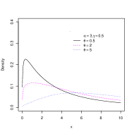
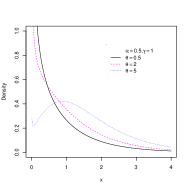
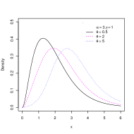
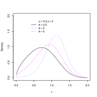
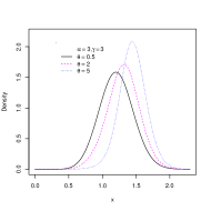
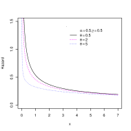
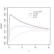
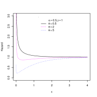
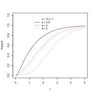
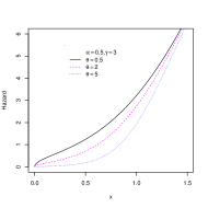
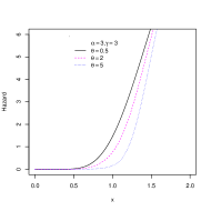
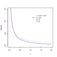
The plots of density and hazard rate functions of EWP distribution for Ξ²=1𝛽1\beta=1 and different values (Ξ±,Ξ³,ΞΈ)π›Όπ›Ύπœƒ(\alpha,\gamma,\theta) are given in Figs. 1 and 2, respectively.
Refer to caption
Refer to caption
Refer to caption
Refer to caption
Refer to caption
Refer to caption
Figure 1: Plots of density function of EWP distribution for Ξ²=1𝛽1\beta=1 and different values α𝛼\alpha, ΞΈπœƒ\theta and γ𝛾\gamma.
Refer to caption
Refer to caption
Refer to caption
Refer to caption
Refer to caption
Refer to caption
Figure 2: Plots of hazard function of EWP distribution for Ξ²=1𝛽1\beta=1 and different values α𝛼\alpha, ΞΈπœƒ\theta and γ𝛾\gamma.
Proposition 1

The limiting distribution of EWP (Ξ±,Ξ²,Ξ³,ΞΈ)π›Όπ›½π›Ύπœƒ(\alpha,\beta,\gamma,\theta) where ΞΈβ†’0+β†’πœƒsuperscript0\theta\rightarrow 0^{+} is

limΞΈβ†’0+F​(y)=β€Žβ€‹(1βˆ’eβˆ’(β€Žβ€‹Ξ²β€‹yβ€‹β€Ž)β€Žβ€‹Ξ³β€‹β€Ž)β€Žβ€‹Ξ±β€‹β€Žβ€‹β€Ž,subscriptβ†’πœƒsuperscript0πΉπ‘¦β€Žsuperscript1superscript𝑒superscriptβ€Žπ›½π‘¦β€Žβ€Žπ›Ύβ€Žβ€Žπ›Όβ€Žβ€Ž\lim_{\theta\rightarrow 0^{+}}F(y)=β€Ž(1-e^{-(β€Ž\beta yβ€Ž)^{β€Ž\gammaβ€Ž}})^{β€Ž\alphaβ€Ž}β€Ž,

which is the cdf of EW distribution.

Proposition 2

The limiting behavior of hazard function of EWP distribution in (6) is
(i) for 0<Ξ³<10𝛾10<\gamma<1, limyβ†’0h​(y)={∞0<α≀10Ξ±>1,subscript→𝑦0β„Žπ‘¦cases0𝛼10𝛼1\lim_{y\rightarrow 0}h(y)=\left\{\begin{array}[]{lc}\infty&0<\alpha\leq 1\\ 0&\alpha>1,\end{array}\right. and limyβ†’βˆžh​(y)=0.subscriptβ†’π‘¦β„Žπ‘¦0\lim_{y\rightarrow\infty}h(y)=0.
(ii) for Ξ³=1𝛾1\gamma=1, limyβ†’0h​(y)={∞0<Ξ±<1θ​βeΞΈβˆ’1Ξ±=10Ξ±>1,subscript→𝑦0β„Žπ‘¦cases0𝛼1πœƒπ›½superscriptπ‘’πœƒ1𝛼10𝛼1\lim_{y\rightarrow 0}h(y)=\left\{\begin{array}[]{lc}\infty&0<\alpha<1\\ \frac{\theta\beta}{e^{\theta}-1}&\alpha=1\\ 0&\alpha>1,\end{array}\right. and limyβ†’βˆžh​(y)=Ξ².subscriptβ†’π‘¦β„Žπ‘¦π›½\lim_{y\rightarrow\infty}h(y)=\beta.
(iii) for Ξ³>1𝛾1\gamma>1, limyβ†’0h​(y)=0,subscript→𝑦0β„Žπ‘¦0\lim_{y\rightarrow 0}h(y)=0, for each value Ξ±>0𝛼0\alpha>0 and limyβ†’βˆžh​(y)=∞subscriptβ†’π‘¦β„Žπ‘¦\lim_{y\rightarrow\infty}h(y)=\infty.

Proof 1

The proof is a forward calculation and is omitted.

4 Quantiles and moments of the EWP distribution

Some of the most important features and characteristics of a distribution can be studied through its moments and quantiles such as tending, dispersion, skewness and kurtosis. Also, the quantiles of a distribution can be used in data generation from a distribution.

The p𝑝pth quantile of the EWP distribution is given by

xp=1β€Žβ€‹Ξ²β€‹β€Žβ€‹β€Žβ€‹[βˆ’log⁑(1βˆ’(β€Žβ€‹1β€Žβ€‹ΞΈβ€‹β€Žβ€‹log⁑(p​(eβ€Žβ€‹ΞΈβ€‹β€Žβˆ’1)+1)β€‹β€Ž)1/β€Žβ€‹Ξ±β€‹β€Ž)]1/β€Žβ€‹Ξ³β€‹β€Ž,subscriptπ‘₯𝑝1β€Žπ›½β€Žβ€Žsuperscriptdelimited-[]1superscriptβ€Ž1β€Žπœƒβ€Žπ‘superscriptπ‘’β€Žπœƒβ€Ž11β€Ž1β€Žπ›Όβ€Ž1β€Žπ›Ύβ€Žx_{p}=\frac{1}{β€Ž\betaβ€Ž}β€Ž\left[-\log\left(1-\left(β€Ž\frac{1}{β€Ž\thetaβ€Ž}\log\left(p\left(e^{β€Ž\thetaβ€Ž}-1\right)+1\right)β€Ž\right)^{1/β€Ž\alphaβ€Ž}\right)\right]^{1/β€Ž\gammaβ€Ž}, (7)

which is used for data generation from the EWP distribution.
Now we obtain the moment generating function of the EWP distribution. Suppose that Y∼E​W​P​(Ξ±,Ξ²,Ξ³,ΞΈ)similar-toπ‘ŒπΈπ‘Šπ‘ƒπ›Όπ›½π›ΎπœƒY\sim EWP(\alpha,\beta,\gamma,\theta) and X(n)=max⁑(X1,β‹―,Xn)subscript𝑋𝑛subscript𝑋1β‹―subscript𝑋𝑛X_{(n)}=\max(X_{1},\cdots,X_{n}), where Xi∼E​W​(Ξ±,Ξ²,Ξ³)similar-tosubscriptπ‘‹π‘–πΈπ‘Šπ›Όπ›½π›ΎX_{i}\sim EW(\alpha,\beta,\gamma) for i=1,2,β‹―,n𝑖12⋯𝑛i=1,2,\cdots,n, then

MY​(t)=βˆ‘n=1∞P​(N=n)​MX(n)​(t)=βˆ‘n=1∞P​(N=n)β€‹βˆ‘k=0∞tkk!​nβ€‹Ξ±β€‹Ξ²βˆ’k​Γ​(1+kΞ³)β€‹βˆ‘j=0∞(βˆ’1)j​(nβ€‹Ξ±βˆ’1j)​(j+1)βˆ’(1+kΞ³)=α​θ(eΞΈβˆ’1)β€‹βˆ‘n=1βˆžβˆ‘k=0βˆžβˆ‘j=0∞(βˆ’1)j​θnβˆ’1(nβˆ’1)!​tkβ€‹Ξ²βˆ’kk!​(nβ€‹Ξ±βˆ’1j)​(j+1)βˆ’(1+kΞ³)​Γ​(1+kΞ³).subscriptπ‘€π‘Œπ‘‘absentsubscriptsuperscript𝑛1𝑃𝑁𝑛subscript𝑀subscript𝑋𝑛𝑑missing-subexpressionabsentsubscriptsuperscript𝑛1𝑃𝑁𝑛subscriptsuperscriptπ‘˜0superscriptπ‘‘π‘˜π‘˜π‘›π›Όsuperscriptπ›½π‘˜Ξ“1π‘˜π›Ύsubscriptsuperscript𝑗0superscript1𝑗binomial𝑛𝛼1𝑗superscript𝑗11π‘˜π›Ύmissing-subexpressionabsentπ›Όπœƒsuperscriptπ‘’πœƒ1subscriptsuperscript𝑛1subscriptsuperscriptπ‘˜0subscriptsuperscript𝑗0superscript1𝑗superscriptπœƒπ‘›1𝑛1superscriptπ‘‘π‘˜superscriptπ›½π‘˜π‘˜binomial𝑛𝛼1𝑗superscript𝑗11π‘˜π›ΎΞ“1π‘˜π›Ύ\begin{array}[b]{ll}M_{Y}(t)&=\sum^{\infty}_{n=1}P(N=n)M_{X_{(n)}}(t)\vskip 6.0pt plus 2.0pt minus 2.0pt\\ &=\sum^{\infty}_{n=1}P(N=n)\sum^{\infty}_{k=0}\frac{t^{k}}{k!}n\alpha\beta^{-k}\Gamma(1+\frac{k}{\gamma})\sum^{\infty}_{j=0}(-1)^{j}{n\alpha-1\choose j}(j+1)^{-(1+\frac{k}{\gamma})}\vskip 6.0pt plus 2.0pt minus 2.0pt\\ &=\frac{\alpha\theta}{(e^{\theta}-1)}\sum^{\infty}_{n=1}\sum^{\infty}_{k=0}\sum^{\infty}_{j=0}(-1)^{j}\frac{\theta^{n-1}}{(n-1)!}\frac{t^{k}\beta^{-k}}{k!}{n\alpha-1\choose j}(j+1)^{-(1+\frac{k}{\gamma})}\Gamma(1+\frac{k}{\gamma}).\end{array} (8)

One can use MY​(t)subscriptπ‘€π‘Œπ‘‘M_{Y}(t) to obtain the kπ‘˜kth moment about zero of the EWP distribution. We have

E​(Yk)=βˆ‘n=1∞P​(N=n)​E​(X(n)k)=α​θβk​(eΞΈβˆ’1)β€‹βˆ‘n=1∞θnβˆ’1(nβˆ’1)!β€‹Ξ±β€‹Ξ²βˆ’kβ€‹βˆ‘j=0∞(βˆ’1)j​(nβ€‹Ξ±βˆ’1j)​(j+1)βˆ’(1+kΞ³)​Γ​(1+kΞ³)=α​θ​Γ​(1+kΞ³)Ξ²k​(eΞΈβˆ’1)β€‹βˆ‘n=1βˆžβˆ‘j=0∞(βˆ’1)j​(nβ€‹Ξ±βˆ’1j)​θnβˆ’1(nβˆ’1)!​(j+1)βˆ’(1+kΞ³).𝐸superscriptπ‘Œπ‘˜absentsubscriptsuperscript𝑛1𝑃𝑁𝑛𝐸subscriptsuperscriptπ‘‹π‘˜π‘›missing-subexpressionabsentπ›Όπœƒsuperscriptπ›½π‘˜superscriptπ‘’πœƒ1subscriptsuperscript𝑛1superscriptπœƒπ‘›1𝑛1𝛼superscriptπ›½π‘˜subscriptsuperscript𝑗0superscript1𝑗binomial𝑛𝛼1𝑗superscript𝑗11π‘˜π›ΎΞ“1π‘˜π›Ύmissing-subexpressionabsentπ›ΌπœƒΞ“1π‘˜π›Ύsuperscriptπ›½π‘˜superscriptπ‘’πœƒ1subscriptsuperscript𝑛1subscriptsuperscript𝑗0superscript1𝑗binomial𝑛𝛼1𝑗superscriptπœƒπ‘›1𝑛1superscript𝑗11π‘˜π›Ύ\begin{array}[b]{ll}E(Y^{k})&=\sum^{\infty}_{n=1}P(N=n)E(X^{k}_{(n)})\vskip 6.0pt plus 2.0pt minus 2.0pt\\ &=\frac{\alpha\theta}{\beta^{k}(e^{\theta}-1)}\sum^{\infty}_{n=1}\frac{\theta^{n-1}}{(n-1)!}\alpha\beta^{-k}\sum^{\infty}_{j=0}(-1)^{j}{n\alpha-1\choose j}(j+1)^{-(1+\frac{k}{\gamma})}\Gamma(1+\frac{k}{\gamma})\vskip 6.0pt plus 2.0pt minus 2.0pt\\ &=\frac{\alpha\theta\Gamma(1+\frac{k}{\gamma})}{\beta^{k}(e^{\theta}-1)}\sum^{\infty}_{n=1}\sum^{\infty}_{j=0}(-1)^{j}{n\alpha-1\choose j}\frac{\theta^{n-1}}{(n-1)!}(j+1)^{-(1+\frac{k}{\gamma})}.\end{array} (9)

Using the change of variable i=nβˆ’1,𝑖𝑛1i=n-1, another equivalent formula for E​(Yk)𝐸superscriptπ‘Œπ‘˜E(Y^{k}) is given by

E​(Yk)=α​θ​Γ​(1+kΞ³)Ξ²k​(eΞΈβˆ’1)β€‹βˆ‘i=0βˆžβˆ‘j=0∞(βˆ’1)j​(α​(i+1)βˆ’1j)​θii!​(j+1)βˆ’(1+kΞ³).𝐸superscriptπ‘Œπ‘˜π›ΌπœƒΞ“1π‘˜π›Ύsuperscriptπ›½π‘˜superscriptπ‘’πœƒ1subscriptsuperscript𝑖0subscriptsuperscript𝑗0superscript1𝑗binomial𝛼𝑖11𝑗superscriptπœƒπ‘–π‘–superscript𝑗11π‘˜π›ΎE(Y^{k})=\frac{\alpha\theta\Gamma(1+\frac{k}{\gamma})}{\beta^{k}(e^{\theta}-1)}\sum^{\infty}_{i=0}\sum^{\infty}_{j=0}(-1)^{j}{\alpha(i+1)-1\choose j}\frac{\theta^{i}}{i!}(j+1)^{-(1+\frac{k}{\gamma})}. (10)

The mean and variance of the EWP distribution are given, respectively, by

E​(Y)=α​θ​Γ​(1+1Ξ³)β​(eΞΈβˆ’1)β€‹βˆ‘n=1βˆžβˆ‘j=0∞(βˆ’1)j​θnβˆ’1(nβˆ’1)!​(nβ€‹Ξ±βˆ’1j)​(j+1)βˆ’(1+1Ξ³),πΈπ‘Œπ›ΌπœƒΞ“11𝛾𝛽superscriptπ‘’πœƒ1subscriptsuperscript𝑛1subscriptsuperscript𝑗0superscript1𝑗superscriptπœƒπ‘›1𝑛1binomial𝑛𝛼1𝑗superscript𝑗111𝛾E(Y)=\frac{\alpha\theta\Gamma(1+\frac{1}{\gamma})}{\beta(e^{\theta}-1)}\sum^{\infty}_{n=1}\sum^{\infty}_{j=0}(-1)^{j}\frac{\theta^{n-1}}{(n-1)!}{n\alpha-1\choose j}(j+1)^{-(1+\frac{1}{\gamma})}, (11)

and

V​a​r​(Y)=α​θ​Γ​(1+2Ξ³)Ξ²2​(eΞΈβˆ’1)β€‹βˆ‘n=1βˆžβˆ‘j=0∞(βˆ’1)j​θnβˆ’1(nβˆ’1)!​(nβ€‹Ξ±βˆ’1j)​(j+1)βˆ’(1+2Ξ³)βˆ’E2​(Y),π‘‰π‘Žπ‘Ÿπ‘Œπ›ΌπœƒΞ“12𝛾superscript𝛽2superscriptπ‘’πœƒ1subscriptsuperscript𝑛1subscriptsuperscript𝑗0superscript1𝑗superscriptπœƒπ‘›1𝑛1binomial𝑛𝛼1𝑗superscript𝑗112𝛾superscript𝐸2π‘Œmissing-subexpression\begin{array}[b]{ll}Var(Y)=\frac{\alpha\theta\Gamma(1+\frac{2}{\gamma})}{\beta^{2}(e^{\theta}-1)}\sum^{\infty}_{n=1}\sum^{\infty}_{j=0}(-1)^{j}\frac{\theta^{n-1}}{(n-1)!}{n\alpha-1\choose j}(j+1)^{-(1+\frac{2}{\gamma})}-E^{2}(Y),\end{array} (12)

where E​(Y)πΈπ‘ŒE(Y) is given in Eq. (11). Note that for positive integer values of α𝛼\alpha, the index j𝑗j in Eqs. (8)-(12) stops at nβ€‹Ξ±βˆ’1𝑛𝛼1n\alpha-1.

5 RΓ©nyi and Shannon entropies

If X𝑋X is a random variable having an absolutely continuous cumulative distribution function F​(x)𝐹π‘₯F(x) and probability distribution function f​(x)𝑓π‘₯f(x), then the basic uncertainty measure for distribution F𝐹F (called the entropy of F𝐹F) is defined as H​(x)=E​[βˆ’log⁑(f​(X))]𝐻π‘₯𝐸delimited-[]𝑓𝑋H(x)=E[-\log(f(X))]. Statistical entropy is a probabilistic measure of uncertainty or ignorance about the outcome of a random experiment, and is a measure of a reduction in that uncertainty. Numerous entropy and information indices, among them the RΓ©nyi entropy, have been developed and used in various disciplines and contexts. Information theoretic principles and methods have become integral parts of probability and statistics and have been applied in various branches of statistics and related fields.

Entropy has been used in various situations in science and engineering. The entropy of a random variable Yπ‘ŒY is a measure of variation of the uncertainty. For a random variable with the pdf f𝑓f, the RΓ©nyi entropy is defined by IR​(r)=11βˆ’r​log⁑{βˆ«β„fr​(y)​𝑑y}subscriptπΌπ‘…π‘Ÿ11π‘Ÿsubscriptℝsuperscriptπ‘“π‘Ÿπ‘¦differential-d𝑦I_{R}(r)=\frac{1}{1-r}\log\{\int_{\mathbb{R}}f^{r}(y)dy\}, for r>0π‘Ÿ0r>0 and rβ‰ 1π‘Ÿ1r\neq 1. Using the power series expansion (1βˆ’z)Ξ±=βˆ‘j=0∞(βˆ’1)j​(Ξ±j)​zjsuperscript1𝑧𝛼superscriptsubscript𝑗0superscript1𝑗binomial𝛼𝑗superscript𝑧𝑗(1-z)^{\alpha}=\sum_{j=0}^{\infty}(-1)^{j}{\alpha\choose j}z^{j} and change of variable (β​y)Ξ³=usuperscript𝛽𝑦𝛾𝑒(\beta y)^{\gamma}=u gives

∫0∞fr​(y)​𝑑y=(β€Žβ€‹β€Žβ€‹Ξ±β€‹β€Žβ€‹Ξ³β€‹β€Žβ€‹ΞΈβ€‹β€Žβ€‹Ξ²β€Žβ€‹Ξ³β€‹β€Žβ€‹β€Žβ€‹β€Žβ€‹β€Žβ€‹β€Žeβ€Žβ€‹ΞΈβˆ’1β€‹β€Žβ€‹β€Ž)rβ€‹βˆ‘j=0βˆžβ€Žβ€‹(rβ€‹β€Žβ€‹ΞΈβ€‹β€Ž)jj!β€‹β€Žβ€‹βˆ‘k=0∞(βˆ’1)k​(β€Žβ€‹Ξ±β€‹(r+j)β€‹β€Žβˆ’rk)β€‹βˆ«0∞yr​(β€Žβ€‹Ξ³βˆ’1β€‹β€Ž)​eβˆ’(r+k)​(β€Žβ€‹Ξ²β€‹yβ€‹β€Ž)β€Žβ€‹Ξ³β€‹β€Žβ€‹π‘‘y.subscriptsuperscript0superscriptπ‘“π‘Ÿπ‘¦differential-d𝑦superscriptβ€Žβ€Žπ›Όβ€Žπ›Ύβ€Žπœƒβ€Žsuperscriptπ›½β€Žπ›Ύβ€Žβ€Žβ€Žβ€Žβ€Žsuperscriptπ‘’β€Žπœƒ1β€Žβ€Žπ‘Ÿsubscriptsuperscript𝑗0β€Žsuperscriptπ‘Ÿβ€Žπœƒβ€Žπ‘—π‘—β€Žsubscriptsuperscriptπ‘˜0superscript1π‘˜binomialβ€Žπ›Όπ‘Ÿπ‘—β€Žπ‘Ÿπ‘˜superscriptsubscript0superscriptπ‘¦π‘Ÿβ€Žπ›Ύ1β€Žsuperscriptπ‘’π‘Ÿπ‘˜superscriptβ€Žπ›½π‘¦β€Žβ€Žπ›Ύβ€Ždifferential-d𝑦missing-subexpression\begin{array}[b]{ll}\int^{\infty}_{0}f^{r}(y)dy=\big{(}β€Ž\frac{β€Ž\alphaβ€Ž\gammaβ€Ž\thetaβ€Ž\beta^{β€Ž\gammaβ€Ž}β€Žβ€Žβ€Žβ€Ž}{e^{β€Ž\theta-1β€Ž}}β€Ž\big{)}^{r}\sum^{\infty}_{j=0}β€Ž\frac{(rβ€Ž\thetaβ€Ž)^{j}}{j!}β€Ž\sum^{\infty}_{k=0}(-1)^{k}{β€Ž\alpha(r+j)β€Ž-r\choose{k}}\int_{0}^{\infty}y^{r(β€Ž\gamma-1β€Ž)}e^{-(r+k)(β€Ž\beta yβ€Ž)^{β€Ž\gammaβ€Ž}}dy.\end{array}

Using formula ∫0∞yr​(β€Žβ€‹Ξ³βˆ’1β€‹β€Ž)​eβˆ’(r+k)​(β€Žβ€‹Ξ²β€‹yβ€‹β€Ž)β€Žβ€‹Ξ³β€‹β€Žβ€‹π‘‘y=Γ​(β€Žβ€‹r​(β€Žβ€‹Ξ³βˆ’1β€‹β€Ž)+1β€Žβ€‹Ξ³β€‹β€Žβ€‹β€Ž)β€‹β€Žβ€‹(β€Žβ€‹Ξ³β€‹β€Žβ€‹Ξ²r(β€ŽΞ³βˆ’1β€Ž)+1)β€Ž)βˆ’1​(r+k)βˆ’(β€Žβ€‹β€Žβ€‹r​(β€Žβ€‹Ξ³βˆ’1β€‹β€Ž)+1β€Žβ€‹Ξ³β€‹β€Žβ€‹β€Ž)\int_{0}^{\infty}y^{r(β€Ž\gamma-1β€Ž)}e^{-(r+k)(β€Ž\beta yβ€Ž)^{β€Ž\gammaβ€Ž}}dy=\Gamma(β€Ž\frac{r(β€Ž\gamma-1β€Ž)+1}{β€Ž\gammaβ€Ž}β€Ž)β€Ž\big{(}β€Ž\gammaβ€Ž\beta^{r(β€Ž\gamma-1β€Ž)+1)β€Ž}\big{)}^{-1}\big{(}r+k\big{)}^{-(β€Žβ€Ž\frac{r(β€Ž\gamma-1β€Ž)+1}{β€Ž\gammaβ€Ž}β€Ž)}, we have

β€Žβ€‹βˆ«0∞fr​(y)​𝑑y=β€Žβ€‹β€Žβ€‹(Ξ±β€‹β€Žβ€‹ΞΈ)r​(β€Žβ€‹Ξ³β€‹β€Žβ€‹Ξ²)β€Žβ€‹rβˆ’1β€‹β€Žβ€‹β€Žβ€‹β€Žβ€‹β€Žβ€‹β€Ž(eβ€Žβ€‹ΞΈβˆ’1β€‹β€Ž)rβ€‹β€Žβ€‹Ξ“β€‹(β€Žβ€‹r​(β€Žβ€‹Ξ³βˆ’1β€‹β€Ž)+1β€Žβ€‹Ξ³β€‹β€Žβ€‹β€Ž)β€‹β€Žβ€‹βˆ‘j=0βˆžβ€Žβ€‹βˆ‘k=0∞(βˆ’1)k​(rβ€‹β€Žβ€‹ΞΈβ€‹β€Ž)jj!β€‹β€Žβ€‹(β€Žβ€‹Ξ±β€‹(r+j)β€‹β€Žβˆ’rk)​(r+k)βˆ’(β€Žβ€‹β€Žβ€‹r​(β€Žβ€‹Ξ³βˆ’1β€‹β€Ž)+1β€Žβ€‹Ξ³β€‹β€Žβ€‹β€Ž).β€Žsubscriptsuperscript0superscriptπ‘“π‘Ÿπ‘¦differential-d𝑦absentβ€Žβ€Žsuperscriptπ›Όβ€Žπœƒπ‘Ÿsuperscriptβ€Žπ›Ύβ€Žπ›½β€Žπ‘Ÿ1β€Žβ€Žβ€Žβ€Žβ€Žsuperscriptsuperscriptπ‘’β€Žπœƒ1β€Žπ‘Ÿβ€ŽΞ“β€Žπ‘Ÿβ€Žπ›Ύ1β€Ž1β€Žπ›Ύβ€Žβ€Žβ€Žsubscriptsuperscript𝑗0β€Žsubscriptsuperscriptπ‘˜0superscript1π‘˜superscriptπ‘Ÿβ€Žπœƒβ€Žπ‘—π‘—β€Žbinomialβ€Žπ›Όπ‘Ÿπ‘—β€Žπ‘Ÿπ‘˜superscriptπ‘Ÿπ‘˜β€Žβ€Žπ‘Ÿβ€Žπ›Ύ1β€Ž1β€Žπ›Ύβ€Žβ€Ž\begin{array}[b]{ll}β€Ž\int^{\infty}_{0}f^{r}(y)dy&=β€Ž\frac{β€Ž(\alphaβ€Ž\theta)^{r}(β€Ž\gammaβ€Ž\beta)^{β€Žr-1β€Ž}β€Žβ€Žβ€Žβ€Ž}{(e^{β€Ž\theta-1β€Ž})^{r}}β€Ž\Gamma(β€Ž\frac{r(β€Ž\gamma-1β€Ž)+1}{β€Ž\gammaβ€Ž}β€Ž)β€Ž\sum^{\infty}_{j=0}β€Ž\sum^{\infty}_{k=0}\frac{(-1)^{k}(rβ€Ž\thetaβ€Ž)^{j}}{j!}β€Ž{β€Ž\alpha(r+j)β€Ž-r\choose{k}}\big{(}r+k\big{)}^{-(β€Žβ€Ž\frac{r(β€Ž\gamma-1β€Ž)+1}{β€Ž\gammaβ€Ž}β€Ž)}.\end{array}

Thus, according to the definition of RΓ©nyi entropy we have

IR​(r)=11βˆ’r​logβ‘β€Žβ€‹[β€Žβ€‹β€Žβ€‹β€Žβ€‹(Ξ±β€‹β€Žβ€‹ΞΈ)r​(β€Žβ€‹Ξ³β€‹β€Žβ€‹Ξ²)β€Žβ€‹rβˆ’1β€‹β€Žβ€‹β€Žβ€‹β€Žβ€‹β€Žβ€‹β€Ž(eβ€Žβ€‹ΞΈβˆ’1β€‹β€Ž)rβ€‹β€Žβ€‹Ξ“β€‹(β€Žβ€‹r​(β€Žβ€‹Ξ³βˆ’1β€‹β€Ž)+1β€Žβ€‹Ξ³β€‹β€Žβ€‹β€Ž)β€‹β€Žβ€‹βˆ‘j=0βˆžβ€Žβ€‹βˆ‘k=0∞(βˆ’1)k​(rβ€‹β€Žβ€‹ΞΈβ€‹β€Ž)jj!β€‹β€Žβ€‹(β€Žβ€‹Ξ±β€‹(r+j)β€‹β€Žβˆ’rk)​(r+k)βˆ’(β€Žβ€‹β€Žβ€‹r​(β€Žβ€‹Ξ³βˆ’1β€‹β€Ž)+1β€Žβ€‹Ξ³β€‹β€Žβ€‹β€Ž)].subscriptπΌπ‘…π‘Ÿ11π‘Ÿβ€Ždelimited-[]β€Žβ€Žβ€Žsuperscriptπ›Όβ€Žπœƒπ‘Ÿsuperscriptβ€Žπ›Ύβ€Žπ›½β€Žπ‘Ÿ1β€Žβ€Žβ€Žβ€Žβ€Žsuperscriptsuperscriptπ‘’β€Žπœƒ1β€Žπ‘Ÿβ€ŽΞ“β€Žπ‘Ÿβ€Žπ›Ύ1β€Ž1β€Žπ›Ύβ€Žβ€Žβ€Žsubscriptsuperscript𝑗0β€Žsubscriptsuperscriptπ‘˜0superscript1π‘˜superscriptπ‘Ÿβ€Žπœƒβ€Žπ‘—π‘—β€Žbinomialβ€Žπ›Όπ‘Ÿπ‘—β€Žπ‘Ÿπ‘˜superscriptπ‘Ÿπ‘˜β€Žβ€Žπ‘Ÿβ€Žπ›Ύ1β€Ž1β€Žπ›Ύβ€Žβ€ŽI_{R}(r)=\frac{1}{1-r}\logβ€Ž\left[β€Žβ€Ž\frac{β€Ž(\alphaβ€Ž\theta)^{r}(β€Ž\gammaβ€Ž\beta)^{β€Žr-1β€Ž}β€Žβ€Žβ€Žβ€Ž}{(e^{β€Ž\theta-1β€Ž})^{r}}β€Ž\Gamma(β€Ž\frac{r(β€Ž\gamma-1β€Ž)+1}{β€Ž\gammaβ€Ž}β€Ž)β€Ž\sum^{\infty}_{j=0}β€Ž\sum^{\infty}_{k=0}\frac{(-1)^{k}(rβ€Ž\thetaβ€Ž)^{j}}{j!}β€Ž{β€Ž\alpha(r+j)β€Ž-r\choose{k}}\big{(}r+k\big{)}^{-(β€Žβ€Ž\frac{r(β€Ž\gamma-1β€Ž)+1}{β€Ž\gammaβ€Ž}β€Ž)}\right].

The Shannon entropy is defined by E​[βˆ’log⁑[f​(Y)]]𝐸delimited-[]π‘“π‘ŒE[-\log[f(Y)]]. This is a special case derived from limrβ†’1IR​(r)subscriptβ†’π‘Ÿ1subscriptπΌπ‘…π‘Ÿ\lim_{r\rightarrow 1}I_{R}(r).

6 Moments of order statistics

Order statistics make their appearance in many areas of statistical theory and practice. Moments of order statistics play an important role in quality control testing and reliability, where a practitioner needs to predict the failure of future items based on the times of a few early failures. These predictors are often based on moments of order statistics. We now derive an explicit expression for the density function and cumulative distribution function of the rπ‘Ÿrth order statistic Yr:nsubscriptπ‘Œ:π‘Ÿπ‘›Y_{r:n}, in a random sample of size n𝑛n from the EWP distribution.

Let the random variable Yr:nsubscriptπ‘Œ:π‘Ÿπ‘›Y_{r:n} be the rπ‘Ÿrth order statistic (Y1:n≀Y2:n≀⋯≀Yn:n)subscriptπ‘Œ:1𝑛subscriptπ‘Œ:2𝑛⋯subscriptπ‘Œ:𝑛𝑛(Y_{1:n}\leq Y_{2:n}\leq\cdots\leq Y_{n:n}) in a sample of size n𝑛n from a distribution with pdf f(.)f(.) and cdf F(.)F(.), respectively. The pdf of Yr:nsubscriptπ‘Œ:π‘Ÿπ‘›Y_{r:n} for r=1,β‹―,nπ‘Ÿ1⋯𝑛r=1,\cdots,n is given by

fr:n​(y)=1B​(r,nβˆ’r+1)​f​(y)​[F​(y)]rβˆ’1​[1βˆ’F​(y)]nβˆ’r,y>0.formulae-sequencesubscript𝑓:π‘Ÿπ‘›π‘¦1π΅π‘Ÿπ‘›π‘Ÿ1𝑓𝑦superscriptdelimited-[]πΉπ‘¦π‘Ÿ1superscriptdelimited-[]1πΉπ‘¦π‘›π‘Ÿπ‘¦0f_{r:n}(y)=\frac{1}{B(r,n-r+1)}f(y)[F(y)]^{r-1}[1-F(y)]^{n-r},~{}~{}~{}y>0. (13)

Substituting from (3) and (4) into (13) and using the binomial expansion gives

fr:n​(y)=1B​(r,nβˆ’r+1)​α​γ​θ​βγ(eΞΈβˆ’1)n​yΞ³βˆ’1​eβˆ’(β​y)γ​(1βˆ’eβˆ’(β​y)Ξ³)Ξ±βˆ’1Γ—βˆ‘i=0rβˆ’1βˆ‘j=0nβˆ’r(βˆ’1)rβˆ’iβˆ’jβˆ’1(rβˆ’1i)(nβˆ’rj)e(nβˆ’rβˆ’j)​θe(i+j)​θ​(1βˆ’eβˆ’(β​y)Ξ³)Ξ±.\begin{array}[b]{ll}f_{r:n}(y)&=\frac{1}{B(r,n-r+1)}\frac{\alpha\gamma\theta\beta^{\gamma}}{(e^{\theta}-1)^{n}}y^{\gamma-1}e^{-(\beta y)^{\gamma}}(1-e^{-(\beta y)^{\gamma}})^{\alpha-1}\vskip 6.0pt plus 2.0pt minus 2.0pt\\ &~{}~{}~{}\times\sum^{r-1}_{i=0}\sum^{n-r}_{j=0}(-1)^{r-i-j-1}{r-1\choose{i}}{n-r\choose{j}}e^{(n-r-j)\theta}e^{(i+j)\theta(1-e^{-(\beta y)^{\gamma}})^{\alpha}}.\end{array} (14)

Also the cdf of Yr:nsubscriptπ‘Œ:π‘Ÿπ‘›Y_{r:n} is given by

Fr:n​(y)=βˆ‘k=rn(nk)​[F​(y)]k​[1βˆ’F​(y)]nβˆ’k=β€Žβ€‹1(eβ€Žβ€‹ΞΈβ€‹β€Žβˆ’1)nβ€‹β€Žβ€‹βˆ‘k=rnβˆ‘i=0kβˆ‘j=0nβˆ’k(βˆ’1)kβˆ’iβˆ’j​(nk)​(ki)​(nβˆ’kj)​e(nβˆ’kβˆ’j)β€‹β€Žβ€‹ΞΈβ€‹β€Žβ€‹e(i+j)β€‹β€Žβ€‹ΞΈβ€‹(1βˆ’eβˆ’(β€Žβ€‹Ξ²β€‹yβ€‹β€Ž)β€Žβ€‹Ξ³β€‹β€Ž)β€Žβ€‹Ξ±β€‹β€Žβ€‹β€Ž.subscript𝐹:π‘Ÿπ‘›π‘¦absentsubscriptsuperscriptπ‘›π‘˜π‘Ÿbinomialπ‘›π‘˜superscriptdelimited-[]πΉπ‘¦π‘˜superscriptdelimited-[]1πΉπ‘¦π‘›π‘˜missing-subexpressionabsentβ€Ž1superscriptsuperscriptπ‘’β€Žπœƒβ€Ž1π‘›β€Žsubscriptsuperscriptπ‘›π‘˜π‘Ÿsubscriptsuperscriptπ‘˜π‘–0subscriptsuperscriptπ‘›π‘˜π‘—0superscript1π‘˜π‘–π‘—binomialπ‘›π‘˜binomialπ‘˜π‘–binomialπ‘›π‘˜π‘—superscriptπ‘’π‘›π‘˜π‘—β€Žπœƒβ€Žsuperscriptπ‘’π‘–π‘—β€Žπœƒsuperscript1superscript𝑒superscriptβ€Žπ›½π‘¦β€Žβ€Žπ›Ύβ€Žβ€Žπ›Όβ€Žβ€Ž\begin{array}[b]{ll}F_{r:n}(y)&=\sum^{n}_{k=r}{{n}\choose{k}}[F(y)]^{k}[1-F(y)]^{n-k}\vskip 6.0pt plus 2.0pt minus 2.0pt\\ &=β€Ž\frac{1}{(e^{β€Ž\thetaβ€Ž}-1)^{n}}β€Ž\sum^{n}_{k=r}\sum^{k}_{i=0}\sum^{n-k}_{j=0}(-1)^{k-i-j}{{n}\choose{k}}{k\choose{i}}{n-k\choose{j}}e^{(n-k-j)β€Ž\thetaβ€Ž}e^{(i+j)β€Ž\theta(1-e^{-(β€Ž\beta yβ€Ž)^{β€Ž\gammaβ€Ž}})^{β€Ž\alphaβ€Ž}β€Ž}.\end{array} (15)

Using the binomial expansion, after some calculations the kπ‘˜kth moment of the rπ‘Ÿrth order statistic Yr:nsubscriptπ‘Œ:π‘Ÿπ‘›Y_{r:n} is given by

E​(Yr:nk)=α​θB​(r,nβˆ’r+1)β€‹β€Žβ€‹Ξ²kβ€‹β€Žβ€‹Ξ“β€‹(kΞ³+1)β€‹βˆ‘i=0nβˆ’rβ€Žβ€‹(βˆ’1)i(eβ€Žβ€‹ΞΈβˆ’1β€‹β€Ž)r+iβ€‹β€Žβ€‹βˆ‘j=0r+iβˆ’1(βˆ’1)r+iβˆ’jβˆ’1​(r+jβˆ’1j)Γ—βˆ‘l=0βˆžβ€Žβ€Žβ€‹ΞΈlβ€‹β€Žβ€‹(j+1)ll!β€Žβˆ‘t=0∞(βˆ’1)t(β€Žβ€‹Ξ±β€‹(l+1)βˆ’1β€‹β€Žt)(t+1)βˆ’(1+β€Žβ€‹kβ€Žβ€‹Ξ³β€‹β€Žβ€‹β€Ž).\begin{array}[b]{ll}E(Y_{r:n}^{k})&=\frac{\alpha\theta}{B(r,n-r+1)β€Ž\beta^{kβ€Ž}}\Gamma\left(\frac{k}{\gamma}+1\right)\sum^{n-r}_{i=0}β€Ž\frac{(-1)^{i}}{(e^{β€Ž\theta}-1β€Ž)^{r+i}}β€Ž\sum^{r+i-1}_{j=0}(-1)^{r+i-j-1}{r+j-1\choose{j}}\vskip 6.0pt plus 2.0pt minus 2.0pt\\ &~{}~{}\times\sum^{\infty}_{l=0}β€Ž\frac{β€Ž\theta^{l}β€Ž(j+1)^{l}}{l!}β€Ž\sum^{\infty}_{t=0}(-1)^{t}{β€Ž\alpha(l+1)-1β€Ž\choose{t}}(t+1)^{-(1+β€Ž\frac{k}{β€Ž\gammaβ€Ž}β€Ž)}.\end{array} (16)

The pdf and cdf of the smallest and biggest order statistics Y1:nsubscriptπ‘Œ:1𝑛Y_{1:n} and Yn:nsubscriptπ‘Œ:𝑛𝑛Y_{n:n} can be obtained using Eqs. (14) and (15) for special cases r=1π‘Ÿ1r=1 and n𝑛n.
For the smallest order statistics Y1:nsubscriptπ‘Œ:1𝑛Y_{1:n}, we have

f1:n​(y)=n​α​γ​θ​βγ(eΞΈβˆ’1)n​yΞ³βˆ’1​eβˆ’(β​y)γ​(1βˆ’eβˆ’(β​y)Ξ³)Ξ±βˆ’1​eθ​(1βˆ’eβˆ’(β​y)Ξ³)α​(eΞΈβˆ’eθ​(1βˆ’eβˆ’(β​y)Ξ³)Ξ±)nβˆ’1,subscript𝑓:1π‘›π‘¦π‘›π›Όπ›Ύπœƒsuperscript𝛽𝛾superscriptsuperscriptπ‘’πœƒ1𝑛superscript𝑦𝛾1superscript𝑒superscript𝛽𝑦𝛾superscript1superscript𝑒superscript𝛽𝑦𝛾𝛼1superscriptπ‘’πœƒsuperscript1superscript𝑒superscript𝛽𝑦𝛾𝛼superscriptsuperscriptπ‘’πœƒsuperscriptπ‘’πœƒsuperscript1superscript𝑒superscript𝛽𝑦𝛾𝛼𝑛1f_{1:n}(y)=\frac{n\alpha\gamma\theta\beta^{\gamma}}{(e^{\theta}-1)^{n}}y^{\gamma-1}e^{-(\beta y)^{\gamma}}(1-e^{-(\beta y)^{\gamma}})^{\alpha-1}e^{\theta(1-e^{-(\beta y)^{\gamma}})^{\alpha}}\left(e^{\theta}-e^{\theta(1-e^{-(\beta y)^{\gamma}})^{\alpha}}\right)^{n-1},
F1:n​(y)=1βˆ’1(eΞΈβˆ’1)n​(eΞΈβˆ’eθ​(1βˆ’eβˆ’(β​y)Ξ³)Ξ±)n,subscript𝐹:1𝑛𝑦11superscriptsuperscriptπ‘’πœƒ1𝑛superscriptsuperscriptπ‘’πœƒsuperscriptπ‘’πœƒsuperscript1superscript𝑒superscript𝛽𝑦𝛾𝛼𝑛F_{1:n}(y)=1-\frac{1}{(e^{\theta}-1)^{n}}\left(e^{\theta}-e^{\theta(1-e^{-(\beta y)^{\gamma}})^{\alpha}}\right)^{n},

and for the biggest order statistics Yn:nsubscriptπ‘Œ:𝑛𝑛Y_{n:n}, we have

fn:n​(y)=n​α​γ​θ​βγ(eΞΈβˆ’1)n​yΞ³βˆ’1​eβˆ’(β​y)γ​(1βˆ’eβˆ’(β​y)Ξ³)Ξ±βˆ’1​eθ​(1βˆ’eβˆ’(β​y)Ξ³)α​(eθ​(1βˆ’eβˆ’(β​y)Ξ³)Ξ±βˆ’1)nβˆ’1,subscript𝑓:π‘›π‘›π‘¦π‘›π›Όπ›Ύπœƒsuperscript𝛽𝛾superscriptsuperscriptπ‘’πœƒ1𝑛superscript𝑦𝛾1superscript𝑒superscript𝛽𝑦𝛾superscript1superscript𝑒superscript𝛽𝑦𝛾𝛼1superscriptπ‘’πœƒsuperscript1superscript𝑒superscript𝛽𝑦𝛾𝛼superscriptsuperscriptπ‘’πœƒsuperscript1superscript𝑒superscript𝛽𝑦𝛾𝛼1𝑛1f_{n:n}(y)=\frac{n\alpha\gamma\theta\beta^{\gamma}}{(e^{\theta}-1)^{n}}y^{\gamma-1}e^{-(\beta y)^{\gamma}}(1-e^{-(\beta y)^{\gamma}})^{\alpha-1}e^{\theta(1-e^{-(\beta y)^{\gamma}})^{\alpha}}\left(e^{\theta(1-e^{-(\beta y)^{\gamma}})^{\alpha}}-1\right)^{n-1},
Fn:n​(y)=1(eΞΈβˆ’1)n​(eθ​(1βˆ’eβˆ’(β​y)Ξ³)Ξ±βˆ’1)n,subscript𝐹:𝑛𝑛𝑦1superscriptsuperscriptπ‘’πœƒ1𝑛superscriptsuperscriptπ‘’πœƒsuperscript1superscript𝑒superscript𝛽𝑦𝛾𝛼1𝑛F_{n:n}(y)=\frac{1}{(e^{\theta}-1)^{n}}\left(e^{\theta(1-e^{-(\beta y)^{\gamma}})^{\alpha}}-1\right)^{n},

The expectation of the smallest and biggest order statistics Y1:nsubscriptπ‘Œ:1𝑛Y_{1:n} and Yn:nsubscriptπ‘Œ:𝑛𝑛Y_{n:n} can be obtained by setting r=1,nπ‘Ÿ1𝑛r=1,n and k=1π‘˜1k=1 in (16).

7 Residual life function of the EWP distribution

Given that a component survives up to time tβ‰₯0𝑑0t\geq 0, the residual life is the period beyond t𝑑t until the time of failure and defined by the conditional random variable Xβˆ’t​|X>​t𝑋𝑑ket𝑋𝑑X-t|X>t. The mean residual life (MRL) function is an important function in survival analysis, actuarial science, economics and other social sciences and reliability for characterizing lifetime. Although the shape of the failure rate function plays an important role in repair and replacement strategies, the MRL function is more relevant as the latter summarizes the entire residual life function, whereas the former considers only the risk of instantaneous failure. In reliability, it is well known that the MRL function and ratio of two consecutive moments of residual life determine the distribution uniquely (Gupta and Gupta, [18]).

MRL function as well as failure rate function is very important, since each of them can be used to determine a unique corresponding lifetime distribution. Lifetimes can exhibit IMRL (increasing MRL) or DMRL (decreasing MRL). MRL functions that first decreases (increases) and then increases (decreases) are usually called bathtub-shaped (upside-down bathtub), BMRL (UMRL). The relationship between the behaviors of the two functions of a distribution was studied by many authors such as Ghitany [14], Mi [30], Park [37] and Tang et al. [39].
The rπ‘Ÿrth order moment of the residual life of the EWP distribution is given by the general formula

mr​(t)=E​[(Yβˆ’t)r​|Y>​t]=1S​(t)β€‹βˆ«t∞(yβˆ’t)r​f​(y)​𝑑y,subscriptπ‘šπ‘Ÿπ‘‘πΈdelimited-[]superscriptπ‘Œπ‘‘π‘Ÿketπ‘Œπ‘‘1𝑆𝑑superscriptsubscript𝑑superscriptπ‘¦π‘‘π‘Ÿπ‘“π‘¦differential-d𝑦m_{r}(t)=E\left[(Y-t)^{r}|Y>t\right]=\frac{1}{S(t)}\int_{t}^{\infty}(y-t)^{r}f(y)dy,

where S​(t)=1βˆ’F​(t)𝑆𝑑1𝐹𝑑S(t)=1-F(t), is the survival function.
In what seen this onwards, we use the expressions

∫t∞xΞ³+sβˆ’1​eβˆ’(k+1)​(β​x)γ​𝑑x=1γ​βγ+s​(k+1)βˆ’(1+sΞ³)​Γ(1+sΞ³)​((k+1)​(β​t)Ξ³),superscriptsubscript𝑑superscriptπ‘₯𝛾𝑠1superscriptπ‘’π‘˜1superscript𝛽π‘₯𝛾differential-dπ‘₯1𝛾superscript𝛽𝛾𝑠superscriptπ‘˜11𝑠𝛾superscriptΞ“1π‘ π›Ύπ‘˜1superscript𝛽𝑑𝛾\int_{t}^{\infty}x^{\gamma+s-1}e^{-(k+1)(\beta x)^{\gamma}}dx=\frac{1}{\gamma\beta^{\gamma+s}}(k+1)^{-(1+\frac{s}{\gamma})}\Gamma^{(1+\frac{s}{\gamma})}\left((k+1)(\beta t)^{\gamma}\right),

and

∫0txΞ³+sβˆ’1​eβˆ’(k+1)​(β​x)γ​𝑑x=1γ​βγ+s​(k+1)βˆ’(1+sΞ³)​Γ(1+sΞ³)​((k+1)​(β​t)Ξ³),superscriptsubscript0𝑑superscriptπ‘₯𝛾𝑠1superscriptπ‘’π‘˜1superscript𝛽π‘₯𝛾differential-dπ‘₯1𝛾superscript𝛽𝛾𝑠superscriptπ‘˜11𝑠𝛾subscriptΞ“1π‘ π›Ύπ‘˜1superscript𝛽𝑑𝛾\int_{0}^{t}x^{\gamma+s-1}e^{-(k+1)(\beta x)^{\gamma}}dx=\frac{1}{\gamma\beta^{\gamma+s}}(k+1)^{-(1+\frac{s}{\gamma})}\Gamma_{(1+\frac{s}{\gamma})}\left((k+1)(\beta t)^{\gamma}\right),

where Ξ“s​(t)=∫t∞xsβˆ’1​eβˆ’x​𝑑xsuperscriptΓ𝑠𝑑superscriptsubscript𝑑superscriptπ‘₯𝑠1superscript𝑒π‘₯differential-dπ‘₯\Gamma^{s}(t)=\int_{t}^{\infty}x^{s-1}e^{-x}dx is the upper incomplete gamma function and Ξ“s​(t)=∫0txsβˆ’1​eβˆ’x​𝑑xsubscriptΓ𝑠𝑑superscriptsubscript0𝑑superscriptπ‘₯𝑠1superscript𝑒π‘₯differential-dπ‘₯\Gamma_{s}(t)=\int_{0}^{t}x^{s-1}e^{-x}dx is the lower incomplete gamma function.
The rπ‘Ÿrth order moment of the residual life of the EWP distribution is given by

mr​(t)=β€Žβ€‹Ξ±β€‹β€Žβ€‹ΞΈβ€‹β€Žβ€‹β€ŽS​(t)​(eΞΈβˆ’1)β€‹βˆ‘i=0r(βˆ’1)rβˆ’i​(ri)β€‹Ξ²βˆ’i​trβˆ’iβ€‹βˆ‘j=0βˆžβˆ‘k=0∞(βˆ’1)k​θjj!​(k+1)1+iΞ³Γ—(α​(j+1)βˆ’1k)​Γ(1+iΞ³)​((k+1)​(β​t)Ξ³),subscriptπ‘šπ‘Ÿπ‘‘absentβ€Žπ›Όβ€Žπœƒβ€Žβ€Žπ‘†π‘‘superscriptπ‘’πœƒ1superscriptsubscript𝑖0π‘Ÿsuperscript1π‘Ÿπ‘–binomialπ‘Ÿπ‘–superscript𝛽𝑖superscriptπ‘‘π‘Ÿπ‘–superscriptsubscript𝑗0superscriptsubscriptπ‘˜0superscript1π‘˜superscriptπœƒπ‘—π‘—superscriptπ‘˜11𝑖𝛾missing-subexpressionabsentbinomial𝛼𝑗11π‘˜superscriptΞ“1π‘–π›Ύπ‘˜1superscript𝛽𝑑𝛾\begin{array}[b]{ll}m_{r}(t)&=\frac{β€Ž\alphaβ€Ž\thetaβ€Žβ€Ž}{S(t)(e^{\theta}-1)}\sum_{i=0}^{r}(-1)^{r-i}{r\choose i}\beta^{-i}t^{r-i}\sum_{j=0}^{\infty}\sum_{k=0}^{\infty}(-1)^{k}\frac{\theta^{j}}{j!(k+1)^{1+\frac{i}{\gamma}}}\\ &~{}~{}\times{{\alpha(j+1)-1}\choose{k}}\Gamma^{\left(1+\frac{i}{\gamma}\right)}\left((k+1)(\beta t)^{\gamma}\right),\end{array} (17)

where S​(t)𝑆𝑑S(t) (the survival function of Yπ‘ŒY) is given in (5).
For the EWP distribution the MRL function which is obtained by setting r=1π‘Ÿ1r=1 in (17), is given in the following theorem.

Theorem 1

The MRL function of the EWP distribution with cdf (3) is given by

m1​(t)=1S​(t)​α​θβ​(eΞΈβˆ’1)β€‹βˆ‘j=0βˆžβˆ‘k=0∞(βˆ’1)k​θjj!​(k+1)1+1γ​(α​(j+1)βˆ’1k)​Γ(1+1Ξ³)​((k+1)​(β​t)Ξ³)βˆ’t.subscriptπ‘š1𝑑1π‘†π‘‘π›Όπœƒπ›½superscriptπ‘’πœƒ1superscriptsubscript𝑗0superscriptsubscriptπ‘˜0superscript1π‘˜superscriptπœƒπ‘—π‘—superscriptπ‘˜111𝛾binomial𝛼𝑗11π‘˜superscriptΞ“11π›Ύπ‘˜1superscript𝛽𝑑𝛾𝑑m_{1}(t)=\frac{1}{S(t)}\frac{\alpha\theta}{\beta(e^{\theta}-1)}\sum_{j=0}^{\infty}\sum_{k=0}^{\infty}(-1)^{k}\frac{\theta^{j}}{j!(k+1)^{1+\frac{1}{\gamma}}}{{\alpha(j+1)-1}\choose{k}}\Gamma^{\left(1+\frac{1}{\gamma}\right)}((k+1)(\beta t)^{\gamma})-t.

The second moment of the residual life function of the EWP distribution is

m2​(t)=1S​(t){α​θβ2​(eΞΈβˆ’1)[βˆ‘j=0βˆžβˆ‘k=0∞(βˆ’1)kΞΈjj!​(k+1)1+2Ξ³(α​(j+1)βˆ’1k)Ξ“(1+2Ξ³)((k+1)(Ξ²t)Ξ³)βˆ’2Ξ²tβˆ‘j=0βˆžβˆ‘k=0∞(βˆ’1)kΞΈjj!​(k+1)1+1Ξ³(α​(j+1)βˆ’1k)Ξ“(1+1Ξ³)((k+1)(Ξ²t)Ξ³)]}+t2.\begin{array}[b]{ll}m_{2}(t)&=\frac{1}{S(t)}\Big{\{}\frac{\alpha\theta}{\beta^{2}(e^{\theta}-1)}\Big{[}\sum_{j=0}^{\infty}\sum_{k=0}^{\infty}(-1)^{k}\frac{\theta^{j}}{j!(k+1)^{1+\frac{2}{\gamma}}}{{\alpha(j+1)-1}\choose{k}}\Gamma^{\left(1+\frac{2}{\gamma}\right)}((k+1)(\beta t)^{\gamma})\\ &~{}~{}-2\beta t\sum_{j=0}^{\infty}\sum_{k=0}^{\infty}(-1)^{k}\frac{\theta^{j}}{j!(k+1)^{1+\frac{1}{\gamma}}}{{\alpha(j+1)-1}\choose{k}}\Gamma^{\left(1+\frac{1}{\gamma}\right)}((k+1)(\beta t)^{\gamma})\Big{]}\Big{\}}+t^{2}.\end{array}

The variance of the residual life function of the EWP distribution can be obtained using m1​(t)subscriptπ‘š1𝑑m_{1}(t) and m2​(t)subscriptπ‘š2𝑑m_{2}(t).

On the other hand, we analogously discuss the reversed residual life and some of its properties. The reversed residual life can be defined as the conditional random variable tβˆ’X|X≀t𝑑conditional𝑋𝑋𝑑t-X|X\leq t which denotes the time elapsed from the failure of a component given that its life is less than or equal to t𝑑t. This random variable may also be called the inactivity time (or time since failure); for more details one may see Kundu and Nanda [22] and Nanda et al. [35]. Also, in reliability, the mean reversed residual life (MRRL) and ratio of two consecutive moments of reversed residual life characterize the distribution uniquely. Using (4) and (5), the reversed failure (or reversed hazard) rate function of the EWP is given by

r​(y)=f​(y)F​(y)=α​γ​θ​βγ​yΞ³βˆ’1​eβˆ’(β​y)γ​(1βˆ’eβˆ’(β​y)Ξ³)Ξ±βˆ’1​eθ​(1βˆ’eβˆ’(β​y)Ξ³)Ξ±eθ​(1βˆ’eβˆ’(β​y)Ξ³)Ξ±βˆ’1.π‘Ÿπ‘¦π‘“π‘¦πΉπ‘¦π›Όπ›Ύπœƒsuperscript𝛽𝛾superscript𝑦𝛾1superscript𝑒superscript𝛽𝑦𝛾superscript1superscript𝑒superscript𝛽𝑦𝛾𝛼1superscriptπ‘’πœƒsuperscript1superscript𝑒superscript𝛽𝑦𝛾𝛼superscriptπ‘’πœƒsuperscript1superscript𝑒superscript𝛽𝑦𝛾𝛼1r(y)=\frac{f(y)}{F(y)}=\frac{\alpha\gamma\theta\beta^{\gamma}y^{\gamma-1}e^{-(\beta y)^{\gamma}}(1-e^{-(\beta y)^{\gamma}})^{\alpha-1}e^{\theta(1-e^{-(\beta y)^{\gamma}})^{\alpha}}}{e^{\theta(1-e^{-(\beta y)^{\gamma}})^{\alpha}}-1}.

The rπ‘Ÿrth moment of the reversed residual life function can be obtained by the formula

ΞΌr​(t)=E​[(tβˆ’Y)r|Y≀t]=1F​(t)β€‹βˆ«0t(tβˆ’y)r​f​(y)​𝑑y.subscriptπœ‡π‘Ÿπ‘‘πΈdelimited-[]conditionalsuperscriptπ‘‘π‘Œπ‘Ÿπ‘Œπ‘‘1𝐹𝑑superscriptsubscript0𝑑superscriptπ‘‘π‘¦π‘Ÿπ‘“π‘¦differential-d𝑦\mu_{r}(t)=E\left[(t-Y)^{r}|Y\leq t\right]=\frac{1}{F(t)}\int_{0}^{t}(t-y)^{r}f(y)dy.

Hence,

ΞΌr​(t)=1F​(t)​α​θ(eΞΈβˆ’1)β€‹βˆ‘i=0r(βˆ’1)i​(ri)​trβˆ’iβ€‹Ξ²βˆ’iβ€‹βˆ‘j=0βˆžβˆ‘k=0∞(βˆ’1)k​θjj!​(k+1)1+iΞ³Γ—(α​(j+1)βˆ’1k)​Γ(1+iΞ³)​((k+1)​(β​t)Ξ³).subscriptπœ‡π‘Ÿπ‘‘absent1πΉπ‘‘π›Όπœƒsuperscriptπ‘’πœƒ1superscriptsubscript𝑖0π‘Ÿsuperscript1𝑖binomialπ‘Ÿπ‘–superscriptπ‘‘π‘Ÿπ‘–superscript𝛽𝑖superscriptsubscript𝑗0superscriptsubscriptπ‘˜0superscript1π‘˜superscriptπœƒπ‘—π‘—superscriptπ‘˜11𝑖𝛾missing-subexpressionabsentbinomial𝛼𝑗11π‘˜subscriptΞ“1π‘–π›Ύπ‘˜1superscript𝛽𝑑𝛾\begin{array}[b]{ll}\mu_{r}(t)&=\frac{1}{F(t)}\frac{\alpha\theta}{(e^{\theta}-1)}\sum_{i=0}^{r}(-1)^{i}{r\choose i}t^{r-i}\beta^{-i}\sum_{j=0}^{\infty}\sum_{k=0}^{\infty}(-1)^{k}\frac{\theta^{j}}{j!(k+1)^{1+\frac{i}{\gamma}}}\\ &~{}~{}\times{{\alpha(j+1)-1}\choose{k}}\Gamma_{\left(1+\frac{i}{\gamma}\right)}((k+1)(\beta t)^{\gamma}).\end{array} (18)

The mean and second moment of the reversed residual life of the EWP distribution can be obtained by setting r=1π‘Ÿ1r=1 and 222 in (18). Also, using ΞΌ1​(t)subscriptπœ‡1𝑑\mu_{1}(t) and ΞΌ2​(t)subscriptπœ‡2𝑑\mu_{2}(t) one can obtain the variance of the reversed residual life function of the EWP distribution.

8 Probability weighted moments

Probability weighted moments (PWMs) are expectations of certain functions of a random variable defined when the ordinary moments of the random variable exist. The PWMs method can generally be used for estimating parameters of a distribution whose inverse form cannot be expressed explicitly.
Estimates based on PWMs are often considered to be superior to standard moment-based estimates. They are sometimes used when maximum likelihood estimates are unavailable or difficult to compute. They may also be used as starting values for maximum likelihood estimates.

The PWMs method, which has been investigated by many researchers, was originally proposed by Greenwood et al. [17]. Since then it has been used widely in practice and for research purposes. Hosking et al. [20] investigated the properties of parameters estimated by the PWMs method for the generalized extreme value (GEV) distribution using fairly long observed series, and they gave a good summary of the PWMs method. Hosking [21] showed that the PWMs method is superior to the Maximum Likelihood (ML) method in parameter estimations when the extreme value distribution is used for longer return periods.

In this paper we calculate the PWMs of the EWP distribution since they can be used for estimating the EWP parameters. For a random variable with the pdf f(.)f(.) and cdf F(.)F(.), the PWMs function are defined by

Ο„s,r=E​[Xs​F​(X)r]=∫0∞xs​(F​(x))r​f​(x)​𝑑x.subscriptπœπ‘ π‘ŸπΈdelimited-[]superscript𝑋𝑠𝐹superscriptπ‘‹π‘Ÿsubscriptsuperscript0superscriptπ‘₯𝑠superscript𝐹π‘₯π‘Ÿπ‘“π‘₯differential-dπ‘₯\tau_{s,r}=E\left[X^{s}F(X)^{r}\right]=\int^{\infty}_{0}x^{s}(F(x))^{r}f(x)dx.

For the EWP distribution the PWMs are given by

Ο„s,r=α​γ​θ​βγ(eΞΈβˆ’1)r+1β€‹βˆ‘i=0r(βˆ’1)rβˆ’i​(ri)β€‹βˆ«0∞xΞ³+sβˆ’1​eβˆ’(β​x)γ​(1βˆ’eβˆ’(β​x)Ξ³)Ξ±βˆ’1​eθ​(i+1)​(1βˆ’eβˆ’(β​x)Ξ³)α​𝑑x=α​γ​θ​βγ(eΞΈβˆ’1)r+1β€‹βˆ‘i=0r(βˆ’1)rβˆ’i​(ri)β€‹βˆ‘j=0∞θj​(i+1)jj!β€‹βˆ«0∞xΞ³+sβˆ’1​eβˆ’(β​x)γ​(1βˆ’eβˆ’(β​x)Ξ³)α​(j+1)βˆ’1​𝑑x=α​γ​θ​βγ(eΞΈβˆ’1)r+1β€‹βˆ‘i=0r(βˆ’1)rβˆ’i​(ri)β€‹βˆ‘j=0∞θj​(i+1)jj!β€‹βˆ‘k=0∞(βˆ’1)k​(α​(j+1)βˆ’1k)β€‹βˆ«0∞xΞ³+sβˆ’1​eβˆ’(k+1)​(β​x)γ​𝑑x.subscriptπœπ‘ π‘Ÿabsentπ›Όπ›Ύπœƒsuperscript𝛽𝛾superscriptsuperscriptπ‘’πœƒ1π‘Ÿ1superscriptsubscript𝑖0π‘Ÿsuperscript1π‘Ÿπ‘–binomialπ‘Ÿπ‘–superscriptsubscript0superscriptπ‘₯𝛾𝑠1superscript𝑒superscript𝛽π‘₯𝛾superscript1superscript𝑒superscript𝛽π‘₯𝛾𝛼1superscriptπ‘’πœƒπ‘–1superscript1superscript𝑒superscript𝛽π‘₯𝛾𝛼differential-dπ‘₯missing-subexpressionabsentπ›Όπ›Ύπœƒsuperscript𝛽𝛾superscriptsuperscriptπ‘’πœƒ1π‘Ÿ1superscriptsubscript𝑖0π‘Ÿsuperscript1π‘Ÿπ‘–binomialπ‘Ÿπ‘–superscriptsubscript𝑗0superscriptπœƒπ‘—superscript𝑖1𝑗𝑗superscriptsubscript0superscriptπ‘₯𝛾𝑠1superscript𝑒superscript𝛽π‘₯𝛾superscript1superscript𝑒superscript𝛽π‘₯𝛾𝛼𝑗11differential-dπ‘₯missing-subexpressionabsentπ›Όπ›Ύπœƒsuperscript𝛽𝛾superscriptsuperscriptπ‘’πœƒ1π‘Ÿ1superscriptsubscript𝑖0π‘Ÿsuperscript1π‘Ÿπ‘–binomialπ‘Ÿπ‘–superscriptsubscript𝑗0superscriptπœƒπ‘—superscript𝑖1𝑗𝑗superscriptsubscriptπ‘˜0superscript1π‘˜binomial𝛼𝑗11π‘˜superscriptsubscript0superscriptπ‘₯𝛾𝑠1superscriptπ‘’π‘˜1superscript𝛽π‘₯𝛾differential-dπ‘₯\begin{array}[b]{ll}\tau_{s,r}&=\frac{\alpha\gamma\theta\beta^{\gamma}}{(e^{\theta}-1)^{r+1}}\sum_{i=0}^{r}(-1)^{r-i}{r\choose i}\int_{0}^{\infty}x^{\gamma+s-1}e^{-(\beta x)^{\gamma}}(1-e^{-(\beta x)^{\gamma}})^{\alpha-1}e^{\theta(i+1)(1-e^{-(\beta x)^{\gamma}})^{\alpha}}dx\vskip 6.0pt plus 2.0pt minus 2.0pt\\ &=\frac{\alpha\gamma\theta\beta^{\gamma}}{(e^{\theta}-1)^{r+1}}\sum_{i=0}^{r}(-1)^{r-i}{r\choose i}\sum_{j=0}^{\infty}\frac{\theta^{j}(i+1)^{j}}{j!}\int_{0}^{\infty}x^{\gamma+s-1}e^{-(\beta x)^{\gamma}}(1-e^{-(\beta x)^{\gamma}})^{\alpha(j+1)-1}dx\vskip 6.0pt plus 2.0pt minus 2.0pt\\ &=\frac{\alpha\gamma\theta\beta^{\gamma}}{(e^{\theta}-1)^{r+1}}\sum_{i=0}^{r}(-1)^{r-i}{r\choose i}\sum_{j=0}^{\infty}\frac{\theta^{j}(i+1)^{j}}{j!}\sum_{k=0}^{\infty}(-1)^{k}{\alpha(j+1)-1\choose k}\int_{0}^{\infty}x^{\gamma+s-1}e^{-(k+1)(\beta x)^{\gamma}}dx.\end{array}

Using formula ∫0∞xΞ³+sβˆ’1​eβˆ’(k+1)​(β​x)γ​𝑑x=Γ​(1+sΞ³)γ​βγ+s​(k+1)1+sΞ³superscriptsubscript0superscriptπ‘₯𝛾𝑠1superscriptπ‘’π‘˜1superscript𝛽π‘₯𝛾differential-dπ‘₯Ξ“1𝑠𝛾𝛾superscript𝛽𝛾𝑠superscriptπ‘˜11𝑠𝛾\int_{0}^{\infty}x^{\gamma+s-1}e^{-(k+1)(\beta x)^{\gamma}}dx=\frac{\Gamma(1+\frac{s}{\gamma})}{\gamma\beta^{\gamma+s}(k+1)^{1+\frac{s}{\gamma}}}, we have

Ο„s,r=α​θβs​(eΞΈβˆ’1)r+1β€‹βˆ‘i=0r(βˆ’1)rβˆ’i​(ri)β€‹βˆ‘j=0∞θj​(i+1)jj!β€‹βˆ‘k=0∞(βˆ’1)k​(α​(j+1)βˆ’1k)​Γ​(1+sΞ³)(k+1)1+sΞ³.subscriptπœπ‘ π‘Ÿπ›Όπœƒsuperscript𝛽𝑠superscriptsuperscriptπ‘’πœƒ1π‘Ÿ1superscriptsubscript𝑖0π‘Ÿsuperscript1π‘Ÿπ‘–binomialπ‘Ÿπ‘–superscriptsubscript𝑗0superscriptπœƒπ‘—superscript𝑖1𝑗𝑗superscriptsubscriptπ‘˜0superscript1π‘˜binomial𝛼𝑗11π‘˜Ξ“1𝑠𝛾superscriptπ‘˜11𝑠𝛾\tau_{s,r}=\frac{\alpha\theta}{\beta^{s}(e^{\theta}-1)^{r+1}}\sum_{i=0}^{r}(-1)^{r-i}{r\choose i}\sum_{j=0}^{\infty}\frac{\theta^{j}(i+1)^{j}}{j!}\sum_{k=0}^{\infty}(-1)^{k}{\alpha(j+1)-1\choose k}\frac{\Gamma(1+\frac{s}{\gamma})}{(k+1)^{1+\frac{s}{\gamma}}}. (19)
Remark 1

The sth moment of the EWP distribution can be obtained by putting r=0π‘Ÿ0r=0 in (19). Therefore

E​(Xs)=α​θβs​(eΞΈβˆ’1)β€‹βˆ‘j=0∞θj​(i+1)jj!β€‹βˆ‘k=0∞(βˆ’1)k​(α​(j+1)βˆ’1k)​Γ​(1+sΞ³)(k+1)1+sΞ³,𝐸superscriptπ‘‹π‘ π›Όπœƒsuperscript𝛽𝑠superscriptπ‘’πœƒ1superscriptsubscript𝑗0superscriptπœƒπ‘—superscript𝑖1𝑗𝑗superscriptsubscriptπ‘˜0superscript1π‘˜binomial𝛼𝑗11π‘˜Ξ“1𝑠𝛾superscriptπ‘˜11𝑠𝛾E(X^{s})=\frac{\alpha\theta}{\beta^{s}(e^{\theta}-1)}\sum_{j=0}^{\infty}\frac{\theta^{j}(i+1)^{j}}{j!}\sum_{k=0}^{\infty}(-1)^{k}{\alpha(j+1)-1\choose k}\frac{\Gamma(1+\frac{s}{\gamma})}{(k+1)^{1+\frac{s}{\gamma}}},

which is equal to Eq. (10), if s𝑠s is replaced by kπ‘˜k. Also, the mean and variance of the EWP distribution can be obtained by setting s=1𝑠1s=1 and 222 in above equation.

9 Mean deviations

The amount of scatter in a population can be measured by the totality of deviations from the mean and median. The mean deviation from the mean is a robust statistic, being more resilient to outliers in a data set than the standard deviation. In the standard deviation, the distances from the mean are squared, so on average, large deviations are weighted more heavily, and thus outliers can heavily influence it. In the mean deviation from the mean, the magnitude of the distances of a small number of outliers is irrelevant. The mean deviation from the median is a measure of statistical dispersion. It is a more robust estimator of scale than the sample variance or standard deviation. It thus behaves better with distributions without a mean or variance, such as the Cauchy distribution.

For a random variable X𝑋X with pdf f​(x)𝑓π‘₯f(x), cdf F​(x)𝐹π‘₯F(x), mean ΞΌπœ‡\mu and median M𝑀M, the mean deviation from the mean and the mean deviation from the median are defined by

Ξ΄1​(X)=∫0∞|xβˆ’ΞΌ|​f​(x)​𝑑x=2​μ​F​(ΞΌ)βˆ’2​I​(ΞΌ),subscript𝛿1𝑋superscriptsubscript0π‘₯πœ‡π‘“π‘₯differential-dπ‘₯2πœ‡πΉπœ‡2πΌπœ‡\delta_{1}(X)=\int_{0}^{\infty}|x-\mu|f(x)dx=2\mu F(\mu)-2I(\mu),

and

Ξ΄2​(X)=∫0∞|xβˆ’M|​f​(x)​𝑑x=2​M​F​(M)βˆ’M+ΞΌβˆ’2​I​(M),subscript𝛿2𝑋superscriptsubscript0π‘₯𝑀𝑓π‘₯differential-dπ‘₯2π‘€πΉπ‘€π‘€πœ‡2𝐼𝑀\delta_{2}(X)=\int_{0}^{\infty}|x-M|f(x)dx=2MF(M)-M+\mu-2I(M),

respectively, where I​(b)=∫0bx​f​(x)​𝑑x𝐼𝑏subscriptsuperscript𝑏0π‘₯𝑓π‘₯differential-dπ‘₯I(b)=\int^{b}_{0}xf(x)dx

Theorem 2

The Mean deviations function of the EWP distribution are

Ξ΄1​(X)=2eΞΈβˆ’1[ΞΌ(eθ​(1βˆ’e(βˆ’Ξ²β€‹ΞΌ)Ξ³)Ξ±βˆ’1)βˆ’Ξ±β€‹ΞΈΞ²βˆ‘j=0βˆžβˆ‘k=0∞(βˆ’1)kΞΈjj!​(k+1)1+1Ξ³(α​(j+1)βˆ’1k)Γ—Ξ“(1+1Ξ³)((k+1)(Ξ²ΞΌ)Ξ³)],\begin{array}[b]{ll}\delta_{1}(X)&=\frac{2}{e^{\theta}-1}\Big{[}\mu\left(e^{\theta(1-e^{(-\beta\mu)^{\gamma}})^{\alpha}}-1\right)-\frac{\alpha\theta}{\beta}\sum_{j=0}^{\infty}\sum_{k=0}^{\infty}(-1)^{k}\frac{\theta^{j}}{j!(k+1)^{1+\frac{1}{\gamma}}}{{\alpha(j+1)-1}\choose{k}}\\ &~{}~{}~{}\times\Gamma_{\left(1+\frac{1}{\gamma}\right)}((k+1)(\beta\mu)^{\gamma})\Big{]},\end{array}

and

Ξ΄2​(X)=ΞΌβˆ’2​α​θβ​(eΞΈβˆ’1)β€‹βˆ‘j=0βˆžβˆ‘k=0∞(βˆ’1)k​θjj!​(k+1)1+1γ​(α​(j+1)βˆ’1k)​Γ(1+1Ξ³)​((k+1)​(β​M)Ξ³),subscript𝛿2π‘‹πœ‡2π›Όπœƒπ›½superscriptπ‘’πœƒ1superscriptsubscript𝑗0superscriptsubscriptπ‘˜0superscript1π‘˜superscriptπœƒπ‘—π‘—superscriptπ‘˜111𝛾binomial𝛼𝑗11π‘˜subscriptΞ“11π›Ύπ‘˜1superscript𝛽𝑀𝛾\delta_{2}(X)=\mu-2\frac{\alpha\theta}{\beta(e^{\theta}-1)}\sum_{j=0}^{\infty}\sum_{k=0}^{\infty}(-1)^{k}\frac{\theta^{j}}{j!(k+1)^{1+\frac{1}{\gamma}}}{{\alpha(j+1)-1}\choose{k}}\Gamma_{\left(1+\frac{1}{\gamma}\right)}((k+1)(\beta M)^{\gamma}),

where ΞΌπœ‡\mu is given in (11) and M𝑀M can be obtained by setting p=.5𝑝.5p=.5 in (7).

10 Bonferroni and Lorenz curves

Study of income inequality has gained a lot of importance over the last many years. Lorenz curve and the associated Gini index are undoubtedly the most popular indices of income inequality. However, there are certain measures which despite possessing interesting characteristics have not been used often for measuring inequality. Bonferroni curve and scaled total time on test transform are two such measures, which have the advantage of being represented graphically in the unit square and can also be related to the Lorenz curve and Gini ratio (Giorgi, [15]). These two measures have some applications in reliability and life testing as well (Giorgi and Crescenzi, [16]). The Bonferroni and Lorenz curves and Gini index have many applications not only in economics to study income and poverty, but also in other fields like reliability, medicine and insurance.

For a random variable X𝑋X with cdf F(.)F(.), the Bonferroni curve is given by

BF​[F​(x)]=1μ​F​(x)β€‹βˆ«0xu​f​(u)​𝑑u.subscript𝐡𝐹delimited-[]𝐹π‘₯1πœ‡πΉπ‘₯subscriptsuperscriptπ‘₯0𝑒𝑓𝑒differential-d𝑒B_{F}[F(x)]=\frac{1}{\mu F(x)}\int^{x}_{0}uf(u)du.

From the relationship between the Bonferroni curve and the mean residual lifetime, the Bonferroni curve of the EWP distribution is given by

BF​[F​(x)]=α​θβ​μ​(eθ​(1βˆ’e(βˆ’Ξ²β€‹x)Ξ³)Ξ±βˆ’1)[βˆ‘j=0βˆžβˆ‘k=0∞(βˆ’1)kΞΈjj!​(k+1)1+1Ξ³(α​(j+1)βˆ’1k)Γ—Ξ“(1+1Ξ³)((k+1)(Ξ²x)Ξ³)].\begin{array}[]{ll}B_{F}[F(x)]&=\frac{\alpha\theta}{\beta\mu\left(e^{\theta(1-e^{(-\beta x)^{\gamma}})^{\alpha}}-1\right)}\Big{[}\sum_{j=0}^{\infty}\sum_{k=0}^{\infty}(-1)^{k}\frac{\theta^{j}}{j!(k+1)^{1+\frac{1}{\gamma}}}{{\alpha(j+1)-1}\choose{k}}\\ &~{}~{}~{}\times\Gamma_{(1+\frac{1}{\gamma})}((k+1)(\beta x)^{\gamma})\Big{]}.\end{array}

The Lorenz curve of the EWP distribution can be obtained via the expression

LF​[F​(x)]=BF​[F​(x)]​F​(x)=α​θβ​μ​(eΞΈβˆ’1)β€‹βˆ‘j=0βˆžβˆ‘k=0∞(βˆ’1)k​θjj!​(k+1)1+1γ​(α​(j+1)βˆ’1k)Γ—Ξ“(1+1Ξ³)((k+1)(Ξ²x)Ξ³)],\begin{array}[]{ll}L_{F}[F(x)]&=B_{F}[F(x)]F(x)=\frac{\alpha\theta}{\beta\mu(e^{\theta}-1)}\sum_{j=0}^{\infty}\sum_{k=0}^{\infty}(-1)^{k}\frac{\theta^{j}}{j!(k+1)^{1+\frac{1}{\gamma}}}{{\alpha(j+1)-1}\choose{k}}\\ &~{}~{}~{}\times\Gamma_{(1+\frac{1}{\gamma})}((k+1)(\beta x)^{\gamma})\Big{]},\end{array}

where ΞΌπœ‡\mu is the mean of the EWP distribution.
The scaled total time on test transform of a distribution function F𝐹F is defined by

SF​[F​(t)]=1ΞΌβ€‹βˆ«0tS​(u)​𝑑u.subscript𝑆𝐹delimited-[]𝐹𝑑1πœ‡subscriptsuperscript𝑑0𝑆𝑒differential-d𝑒S_{F}[F(t)]=\frac{1}{\mu}\int^{t}_{0}S(u)du.

If F​(t)𝐹𝑑F(t) denotes the cdf of the EWP distribution then

SF​[F​(t)]=1μ​(eΞΈβˆ’1)​[t​eΞΈβˆ’1Ξ³β€‹Ξ²β€‹βˆ‘j=0βˆžβˆ‘k=0∞(βˆ’1)k​θjj!​(α​jk)​kβˆ’1/γ​Γ(1Ξ³)​(k​(β​t)Ξ³)].subscript𝑆𝐹delimited-[]𝐹𝑑1πœ‡superscriptπ‘’πœƒ1delimited-[]𝑑superscriptπ‘’πœƒ1𝛾𝛽subscriptsuperscript𝑗0subscriptsuperscriptπ‘˜0superscript1π‘˜superscriptπœƒπ‘—π‘—binomialπ›Όπ‘—π‘˜superscriptπ‘˜1𝛾subscriptΞ“1π›Ύπ‘˜superscript𝛽𝑑𝛾S_{F}[F(t)]=\frac{1}{\mu(e^{\theta}-1)}\Big{[}te^{\theta}-\frac{1}{\gamma\beta}\sum^{\infty}_{j=0}\sum^{\infty}_{k=0}(-1)^{k}\frac{\theta^{j}}{j!}{{\alpha j}\choose{k}}k^{-1/\gamma}\Gamma_{(\frac{1}{\gamma})}(k(\beta t)^{\gamma})\Big{]}.

The cumulative total time can be obtained by using formula CF=∫01SF​[F​(t)]​f​(t)​𝑑tsubscript𝐢𝐹superscriptsubscript01subscript𝑆𝐹delimited-[]𝐹𝑑𝑓𝑑differential-d𝑑C_{F}=\int_{0}^{1}S_{F}[F(t)]f(t)dt and the Gini index can be derived from the relationship G=1βˆ’CF𝐺1subscript𝐢𝐹G=1-C_{F}.

11 Estimation and inference

In this section, we discuss the estimation of the parameters of the EWP distribution. Let Y1,Y2,β‹―,Ynsubscriptπ‘Œ1subscriptπ‘Œ2β‹―subscriptπ‘Œπ‘›Y_{1},Y_{2},\cdots,Y_{n} be a random sample with observed values y1,y2,β‹―,ynsubscript𝑦1subscript𝑦2β‹―subscript𝑦𝑛y_{1},y_{2},\cdots,y_{n} from EWP distribution with parameters Ξ±,Ξ²,γ𝛼𝛽𝛾\alpha,\beta,\gamma and ΞΈπœƒ\theta. Let Θ=(Ξ±,Ξ²,Ξ³,ΞΈ)TΘsuperscriptπ›Όπ›½π›Ύπœƒπ‘‡\Theta=(\alpha,\beta,\gamma,\theta)^{T} be the parameter vector. The total log-likelihood function is given by

ln≑ln​(y;Θ)=βˆ’n​log⁑[eβ€Žβ€‹ΞΈβ€‹β€Žβˆ’1]+n​[logβ‘β€Žβ€‹β€Žβ€‹ΞΈβ€‹β€Ž+logβ‘β€Žβ€‹Ξ±+logβ‘β€Žβ€‹Ξ³+β€Žβ€‹Ξ³β€‹logβ‘β€Žβ€‹Ξ²β€‹β€Ž]+(β€Žβ€‹Ξ³βˆ’1β€‹β€Ž)β€‹βˆ‘i=1nlog⁑yiβˆ’βˆ‘i=1n(β€Žβ€‹Ξ²β€‹yiβ€‹β€Ž)Ξ³+(β€Žβ€‹Ξ±βˆ’1β€‹β€Ž)β€‹β€Žβ€‹βˆ‘i=1nlog⁑(1βˆ’eβˆ’(β€Žβ€‹Ξ²β€‹yiβ€‹β€Ž)β€Žβ€‹Ξ³β€‹β€Ž)+β€Žβ€‹ΞΈβ€‹β€Žβ€‹βˆ‘i=1n(1βˆ’eβˆ’(β€Žβ€‹Ξ²β€‹yi)β€Žβ€‹Ξ³β€‹β€Ž)β€Žβ€‹Ξ±β€‹β€Ž.subscript𝑙𝑛subscriptπ‘™π‘›π‘¦Ξ˜absent𝑛superscriptπ‘’β€Žπœƒβ€Ž1𝑛delimited-[]β€Žβ€Žπœƒβ€Žβ€Žπ›Όβ€Žπ›Ύβ€Žπ›Ύβ€Žπ›½β€Žmissing-subexpressionβ€Žπ›Ύ1β€Žsubscriptsuperscript𝑛𝑖1subscript𝑦𝑖subscriptsuperscript𝑛𝑖1superscriptβ€Žπ›½subscriptπ‘¦π‘–β€Žπ›Ύβ€Žπ›Ό1β€Žβ€Žsubscriptsuperscript𝑛𝑖11superscript𝑒superscriptβ€Žπ›½subscriptπ‘¦π‘–β€Žβ€Žπ›Ύβ€Žmissing-subexpressionβ€Žπœƒβ€Žsubscriptsuperscript𝑛𝑖1superscript1superscript𝑒superscriptβ€Žπ›½subscriptπ‘¦π‘–β€Žπ›Ύβ€Žβ€Žπ›Όβ€Ž\begin{array}[b]{ll}l_{n}\equiv l_{n}(y;\Theta)&=-n\log[e^{β€Ž\thetaβ€Ž}-1]+n[\logβ€Žβ€Ž\thetaβ€Ž+\logβ€Ž\alpha+\logβ€Ž\gamma+β€Ž\gamma\logβ€Ž\betaβ€Ž]\vskip 6.0pt plus 2.0pt minus 2.0pt\\ &~{}~{}~{}+(β€Ž\gamma-1β€Ž)\sum^{n}_{i=1}\log y_{i}-\sum^{n}_{i=1}(β€Ž\beta y_{i}β€Ž)^{\gamma}+(β€Ž\alpha-1β€Ž)β€Ž\sum^{n}_{i=1}\log(1-e^{-(β€Ž\beta y_{i}β€Ž)^{β€Ž\gammaβ€Ž}})\vskip 6.0pt plus 2.0pt minus 2.0pt\\ &~{}~{}~{}+β€Ž\thetaβ€Ž\sum^{n}_{i=1}(1-e^{-(β€Ž\beta y_{i})^{β€Ž\gammaβ€Ž}})^{β€Ž\alphaβ€Ž}.\end{array}

The associated score function is given by Un​(Θ)=(βˆ‚ln/βˆ‚Ξ±,βˆ‚ln/βˆ‚Ξ²,βˆ‚ln/βˆ‚Ξ³,βˆ‚ln/βˆ‚ΞΈ)Tsubscriptπ‘ˆπ‘›Ξ˜superscriptsubscript𝑙𝑛𝛼subscript𝑙𝑛𝛽subscript𝑙𝑛𝛾subscriptπ‘™π‘›πœƒπ‘‡U_{n}(\Theta)=(\partial l_{n}/\partial\alpha,\partial l_{n}/\partial\beta,\partial l_{n}/\partial\gamma,\partial l_{n}/\partial\theta)^{T}, where

βˆ‚lnβˆ‚Ξ±=β€Žβ€‹nβ€Žβ€‹Ξ±β€‹β€Ž+βˆ‘i=1nlog⁑(1βˆ’eβˆ’(β€Žβ€‹Ξ²β€‹yiβ€‹β€Ž)β€Žβ€‹Ξ³β€‹β€Ž)+β€Žβ€‹ΞΈβ€‹βˆ‘i=1nlog⁑(1βˆ’eβˆ’(β€Žβ€‹Ξ²β€‹yiβ€‹β€Ž)β€Žβ€‹Ξ³β€‹β€Ž)β€‹β€Žβ€‹(1βˆ’eβˆ’(β€Žβ€‹Ξ²β€‹yiβ€‹β€Ž)β€Žβ€‹Ξ³β€‹β€Ž)β€Žβ€‹Ξ±β€‹β€Žβ€‹β€Ž,βˆ‚lnβˆ‚Ξ²=β€Žβ€‹nβ€‹β€Žβ€‹Ξ³β€‹β€Žβ€Žβ€‹Ξ²β€‹β€Žβˆ’β€Žβ€‹Ξ³β€‹β€Žβ€‹Ξ²β€Žβ€‹Ξ³βˆ’1β€‹β€Žβ€‹βˆ‘i=1nyiβ€Žβ€‹Ξ³β€‹β€Ž+(β€Žβ€‹Ξ±βˆ’1β€‹β€Ž)β€‹β€Žβ€‹Ξ³β€‹β€Žβ€‹Ξ²β€Žβ€‹Ξ³βˆ’1β€‹β€Žβ€‹βˆ‘i=1nβ€Žβ€‹yiβ€Žβ€‹Ξ³β€‹β€Žβ€‹eβˆ’(β€Žβ€‹Ξ²β€‹yiβ€‹β€Ž)β€Žβ€‹Ξ³β€‹β€Ž1βˆ’eβˆ’(β€Žβ€‹Ξ²β€‹yiβ€‹β€Ž)β€Žβ€‹Ξ³β€‹β€Ž+β€Žβ€‹ΞΈβ€‹β€Žβ€‹Ξ³β€‹β€Žβ€‹Ξ±β€‹β€Žβ€‹β€Žβ€‹Ξ²β€Žβ€‹Ξ³βˆ’1β€‹β€Žβ€‹β€Žβ€‹β€Žβ€‹β€Žβ€‹β€Žβ€‹β€Žβ€‹β€Žβ€‹β€Žβ€‹β€Žβ€‹β€Žβ€‹βˆ‘i=1nyiβ€Žβ€‹Ξ³β€‹β€Žβ€‹eβˆ’(β€Žβ€‹Ξ²β€‹yiβ€‹β€Ž)β€Žβ€‹Ξ³β€‹β€Žβ€‹(1βˆ’eβˆ’(β€Žβ€‹Ξ²β€‹yiβ€‹β€Ž)β€Žβ€‹Ξ³β€‹β€Ž)β€Žβ€‹Ξ±βˆ’1β€‹β€Ž,βˆ‚lnβˆ‚Ξ³=β€Žβ€‹nβ€Žβ€‹Ξ³β€‹β€Ž+n​logβ‘β€Žβ€‹Ξ²+βˆ‘i=1nlog⁑yiβˆ’βˆ‘i=1n(β€Žβ€‹Ξ²β€‹yiβ€‹β€Ž)β€Žβ€‹Ξ³β€‹β€Žβ€‹log⁑(β€Žβ€‹Ξ²β€‹yiβ€‹β€Ž)β€Žβ€‹β€Ž+(β€Žβ€‹Ξ±βˆ’1β€‹β€Ž)β€‹βˆ‘i=1nβ€Žβ€‹(β€Žβ€‹Ξ²β€‹yiβ€‹β€Ž)β€Žβ€‹Ξ³β€‹β€Žβ€‹log⁑(β€Žβ€‹Ξ²β€‹yiβ€‹β€Ž)β€‹β€Žβ€‹β€Žβ€‹eβˆ’(β€Žβ€‹Ξ²β€‹yiβ€‹β€Ž)β€Žβ€‹Ξ³β€‹β€Ž1βˆ’eβˆ’(β€Žβ€‹Ξ²β€‹yiβ€‹β€Ž)β€Žβ€‹Ξ³β€‹β€Ž+β€Žβ€‹ΞΈβ€‹β€Žβ€‹Ξ±β€‹βˆ‘i=1n(β€Žβ€‹Ξ²β€‹yiβ€‹β€Ž)β€Žβ€‹Ξ³β€‹β€Žβ€‹log⁑(β€Žβ€‹Ξ²β€‹yiβ€‹β€Ž)​eβˆ’(β€Žβ€‹Ξ²β€‹yiβ€‹β€Ž)β€Žβ€‹Ξ³β€‹β€Žβ€‹(1βˆ’eβˆ’(β€Žβ€‹Ξ²β€‹yiβ€‹β€Ž)β€Žβ€‹Ξ³β€‹β€Ž)β€Žβ€‹Ξ±βˆ’1β€‹β€Ž,β€Žβ€‹β€Žβ€‹β€Žβˆ‚lnβˆ‚ΞΈ=β€Žβ€‹nβ€Žβ€‹ΞΈβ€‹β€Ž+βˆ‘i=1n(1βˆ’eβˆ’(β€Žβ€‹Ξ²β€‹yiβ€‹β€Ž)β€Žβ€‹Ξ³β€‹β€Ž)β€Žβ€‹Ξ±β€‹β€Žβˆ’β€Žβ€‹n1βˆ’eβˆ’β€Žβ€‹ΞΈβ€‹β€Žβ€‹β€Žβ€‹β€Ž.subscript𝑙𝑛𝛼absentβ€Žπ‘›β€Žπ›Όβ€Žsubscriptsuperscript𝑛𝑖11superscript𝑒superscriptβ€Žπ›½subscriptπ‘¦π‘–β€Žβ€Žπ›Ύβ€Žβ€Žπœƒsubscriptsuperscript𝑛𝑖11superscript𝑒superscriptβ€Žπ›½subscriptπ‘¦π‘–β€Žβ€Žπ›Ύβ€Žβ€Žsuperscript1superscript𝑒superscriptβ€Žπ›½subscriptπ‘¦π‘–β€Žβ€Žπ›Ύβ€Žβ€Žπ›Όβ€Žβ€Žsubscript𝑙𝑛𝛽absentβ€Žπ‘›β€Žπ›Ύβ€Žβ€Žπ›½β€Žβ€Žπ›Ύβ€Žsuperscriptπ›½β€Žπ›Ύ1β€Žsubscriptsuperscript𝑛𝑖1superscriptsubscriptπ‘¦π‘–β€Žπ›Ύβ€Žβ€Žπ›Ό1β€Žβ€Žπ›Ύβ€Žsuperscriptπ›½β€Žπ›Ύ1β€Žsubscriptsuperscript𝑛𝑖1β€Žsuperscriptsubscriptπ‘¦π‘–β€Žπ›Ύβ€Žsuperscript𝑒superscriptβ€Žπ›½subscriptπ‘¦π‘–β€Žβ€Žπ›Ύβ€Ž1superscript𝑒superscriptβ€Žπ›½subscriptπ‘¦π‘–β€Žβ€Žπ›Ύβ€Žmissing-subexpressionβ€Žπœƒβ€Žπ›Ύβ€Žπ›Όβ€Žβ€Žsuperscriptπ›½β€Žπ›Ύ1β€Žβ€Žβ€Žβ€Žβ€Žβ€Žβ€Žβ€Žβ€Žβ€Žsubscriptsuperscript𝑛𝑖1superscriptsubscriptπ‘¦π‘–β€Žπ›Ύβ€Žsuperscript𝑒superscriptβ€Žπ›½subscriptπ‘¦π‘–β€Žβ€Žπ›Ύβ€Žsuperscript1superscript𝑒superscriptβ€Žπ›½subscriptπ‘¦π‘–β€Žβ€Žπ›Ύβ€Žβ€Žπ›Ό1β€Žsubscript𝑙𝑛𝛾absentβ€Žπ‘›β€Žπ›Ύβ€Žπ‘›β€Žπ›½subscriptsuperscript𝑛𝑖1subscript𝑦𝑖subscriptsuperscript𝑛𝑖1superscriptβ€Žπ›½subscriptπ‘¦π‘–β€Žβ€Žπ›Ύβ€Žβ€Žπ›½subscriptπ‘¦π‘–β€Žmissing-subexpressionβ€Žβ€Žβ€Žπ›Ό1β€Žsubscriptsuperscript𝑛𝑖1β€Žsuperscriptβ€Žπ›½subscriptπ‘¦π‘–β€Žβ€Žπ›Ύβ€Žβ€Žπ›½subscriptπ‘¦π‘–β€Žβ€Žβ€Žsuperscript𝑒superscriptβ€Žπ›½subscriptπ‘¦π‘–β€Žβ€Žπ›Ύβ€Ž1superscript𝑒superscriptβ€Žπ›½subscriptπ‘¦π‘–β€Žβ€Žπ›Ύβ€Žβ€Žπœƒβ€Žπ›Όsubscriptsuperscript𝑛𝑖1superscriptβ€Žπ›½subscriptπ‘¦π‘–β€Žβ€Žπ›Ύβ€Žβ€Žπ›½subscriptπ‘¦π‘–β€Žsuperscript𝑒superscriptβ€Žπ›½subscriptπ‘¦π‘–β€Žβ€Žπ›Ύβ€Žsuperscript1superscript𝑒superscriptβ€Žπ›½subscriptπ‘¦π‘–β€Žβ€Žπ›Ύβ€Žβ€Žπ›Ό1β€Žβ€Žβ€Žβ€Žsubscriptπ‘™π‘›πœƒabsentβ€Žπ‘›β€Žπœƒβ€Žsubscriptsuperscript𝑛𝑖1superscript1superscript𝑒superscriptβ€Žπ›½subscriptπ‘¦π‘–β€Žβ€Žπ›Ύβ€Žβ€Žπ›Όβ€Žβ€Žπ‘›1superscriptπ‘’β€Žπœƒβ€Žβ€Žβ€Ž\begin{array}[]{ll}\frac{\partial l_{n}}{\partial\alpha}&=β€Ž\frac{n}{β€Ž\alphaβ€Ž}+\sum^{n}_{i=1}\log(1-e^{-(β€Ž\beta y_{i}β€Ž)^{β€Ž\gammaβ€Ž}})+β€Ž\theta\sum^{n}_{i=1}\log(1-e^{-(β€Ž\beta y_{i}β€Ž)^{β€Ž\gammaβ€Ž}})β€Ž(1-e^{-(β€Ž\beta y_{i}β€Ž)^{β€Ž\gammaβ€Ž}})^{β€Ž\alphaβ€Ž}β€Ž,\vskip 6.0pt plus 2.0pt minus 2.0pt\\ \frac{\partial l_{n}}{\partial\beta}&=β€Ž\frac{nβ€Ž\gammaβ€Ž}{β€Ž\betaβ€Ž}-β€Ž\gammaβ€Ž\beta^{β€Ž\gamma-1β€Ž}\sum^{n}_{i=1}y_{i}^{β€Ž\gammaβ€Ž}+(β€Ž\alpha-1β€Ž)β€Ž\gammaβ€Ž\beta^{β€Ž\gamma-1β€Ž}\sum^{n}_{i=1}β€Ž\frac{y_{i}^{β€Ž\gammaβ€Ž}e^{-(β€Ž\beta y_{i}β€Ž)^{β€Ž\gammaβ€Ž}}}{1-e^{-(β€Ž\beta y_{i}β€Ž)^{β€Ž\gammaβ€Ž}}}\vskip 6.0pt plus 2.0pt minus 2.0pt\\ &~{}~{}+β€Ž\thetaβ€Ž\gammaβ€Ž\alphaβ€Žβ€Ž\beta^{β€Ž\gamma-1β€Ž}β€Žβ€Žβ€Žβ€Žβ€Žβ€Žβ€Žβ€Žβ€Ž\sum^{n}_{i=1}y_{i}^{β€Ž\gammaβ€Ž}e^{-(β€Ž\beta y_{i}β€Ž)^{β€Ž\gammaβ€Ž}}(1-e^{-(β€Ž\beta y_{i}β€Ž)^{β€Ž\gammaβ€Ž}})^{β€Ž\alpha-1β€Ž},\vskip 6.0pt plus 2.0pt minus 2.0pt\\ \frac{\partial l_{n}}{\partial\gamma}&=β€Ž\frac{n}{β€Ž\gammaβ€Ž}+n\logβ€Ž\beta+\sum^{n}_{i=1}\log y_{i}-\sum^{n}_{i=1}(β€Ž\beta y_{i}β€Ž)^{β€Ž\gammaβ€Ž}\log(β€Ž\beta y_{i}β€Ž)\vskip 6.0pt plus 2.0pt minus 2.0pt\\ &~{}~{}β€Žβ€Ž+(β€Ž\alpha-1β€Ž)\sum^{n}_{i=1}β€Ž\frac{(β€Ž\beta y_{i}β€Ž)^{β€Ž\gammaβ€Ž}\log(β€Ž\beta y_{i}β€Ž)β€Žβ€Že^{-(β€Ž\beta y_{i}β€Ž)^{β€Ž\gammaβ€Ž}}}{1-e^{-(β€Ž\beta y_{i}β€Ž)^{β€Ž\gammaβ€Ž}}}+β€Ž\thetaβ€Ž\alpha\sum^{n}_{i=1}(β€Ž\beta y_{i}β€Ž)^{β€Ž\gammaβ€Ž}\log(β€Ž\beta y_{i}β€Ž)e^{-(β€Ž\beta y_{i}β€Ž)^{β€Ž\gammaβ€Ž}}(1-e^{-(β€Ž\beta y_{i}β€Ž)^{β€Ž\gammaβ€Ž}})^{β€Ž\alpha-1β€Ž},β€Žβ€Žβ€Ž\vskip 6.0pt plus 2.0pt minus 2.0pt\\ \frac{\partial l_{n}}{\partial\theta}&=β€Ž\frac{n}{β€Ž\thetaβ€Ž}+\sum^{n}_{i=1}(1-e^{-(β€Ž\beta y_{i}β€Ž)^{β€Ž\gammaβ€Ž}})^{β€Ž\alphaβ€Ž}-β€Ž\frac{n}{1-e^{-β€Ž\thetaβ€Ž}}β€Žβ€Ž.\end{array}

The MLE of ΘΘ\Theta, say Θ^^Θ\widehat{\Theta}, is obtained by solving the nonlinear system Un​(Θ)=0subscriptπ‘ˆπ‘›Ξ˜0U_{n}\left(\Theta\right)=\textbf{0}. The solution of this nonlinear system of equation has not a closed form. For interval estimation and hypothesis tests on the model parameters, we require the information matrix. The 4Γ—4444\times 4 observed information matrix is

In​(Θ)=βˆ’[Iα​αIα​βIα​γIα​θIα​βIβ​βIβ​γIβ​θIα​γIβ​γIγ​γIγ​θIα​θIβ​θIγ​θIθ​θ],subscriptπΌπ‘›Ξ˜delimited-[]subscript𝐼𝛼𝛼subscript𝐼𝛼𝛽subscript𝐼𝛼𝛾subscriptπΌπ›Όπœƒsubscript𝐼𝛼𝛽subscript𝐼𝛽𝛽subscript𝐼𝛽𝛾subscriptπΌπ›½πœƒsubscript𝐼𝛼𝛾subscript𝐼𝛽𝛾subscript𝐼𝛾𝛾subscriptπΌπ›ΎπœƒsubscriptπΌπ›ΌπœƒsubscriptπΌπ›½πœƒsubscriptπΌπ›ΎπœƒsubscriptπΌπœƒπœƒI_{n}\left(\Theta\right)=-\left[\begin{array}[]{cccc}I_{\alpha\alpha}&I_{\alpha\beta}&I_{\alpha\gamma}&I_{\alpha\theta}\\ I_{\alpha\beta}&I_{\beta\beta}&I_{\beta\gamma}&I_{\beta\theta}\\ I_{\alpha\gamma}&I_{\beta\gamma}&I_{\gamma\gamma}&I_{\gamma\theta}\\ I_{\alpha\theta}&I_{\beta\theta}&I_{\gamma\theta}&I_{\theta\theta}\\ \end{array}\right],

whose elements are given in Appendix.

Applying the usual large sample approximation, MLE of ΘΘ\Theta i.e. Θ^^Θ\widehat{\Theta} can be treated as being approximately N4​(Θ,Jn​(Θ)βˆ’1)subscript𝑁4Θsubscript𝐽𝑛superscriptΘ1N_{4}(\Theta,{J_{n}(\Theta)}^{-1}{\mathbf{)}}, where Jn​(Θ)=E​[In​(Θ)]subscriptπ½π‘›Ξ˜πΈdelimited-[]subscriptπΌπ‘›Ξ˜J_{n}\left(\Theta\right)=E\left[I_{n}\left(\Theta\right)\right]. Under conditions that are fulfilled for parameters in the interior of the parameter space but not on the boundary, the asymptotic distribution of n​(Θ^βˆ’Ξ˜)𝑛^ΘΘ\sqrt{n}(\widehat{\Theta}{\rm-}\Theta{\rm)} is N4​(𝟎,J​(Θ)βˆ’1)subscript𝑁40𝐽superscriptΘ1N_{4}({\mathbf{0}},{J(\Theta)}^{-1}), where J​(Θ)=limnβ†’βˆžnβˆ’1​In​(Θ)𝐽Θsubscript→𝑛superscript𝑛1subscriptπΌπ‘›Ξ˜J\left(\Theta\right)={\mathop{\lim}_{n\to\infty}{n^{-1}I}_{n}(\Theta)\ } is the unit information matrix. This asymptotic behavior remains valid if J​(Θ)𝐽ΘJ(\Theta) is replaced by the average sample information matrix evaluated at Θ^^Θ\widehat{\Theta}, say nβˆ’1​In​(Θ^)superscript𝑛1subscript𝐼𝑛^Θ{n^{-1}I}_{n}(\widehat{\Theta}). The estimated asymptotic multivariate normal N4​(Θ,In​(Θ^)βˆ’1)subscript𝑁4Θsubscript𝐼𝑛superscript^Θ1N_{4}(\Theta,{I_{n}(\widehat{\Theta})}^{-1}) distribution of Θ^^Θ\widehat{\Theta} can be used to construct approximate confidence intervals for the parameters and for the hazard rate and survival functions. A 100​(1βˆ’Ξ³)1001𝛾100(1-\gamma) asymptotic confidence interval for each parameter ΘrsubscriptΘr{\Theta}_{{\rm r}} is given by

A​C​Ir=(Θ^rβˆ’ZΞ³2​I^r​r,Θ^r+ZΞ³2​I^r​r),𝐴𝐢subscriptπΌπ‘Ÿsubscript^Ξ˜π‘Ÿsubscript𝑍𝛾2superscript^πΌπ‘Ÿπ‘Ÿsubscript^Ξ˜π‘Ÿsubscript𝑍𝛾2superscript^πΌπ‘Ÿπ‘Ÿ{ACI}_{r}=({\widehat{\Theta}}_{r}-Z_{\frac{\gamma}{2}}\sqrt{{\hat{I}}^{rr}},{\widehat{\Theta}}_{r}+Z_{\frac{\gamma}{2}}\sqrt{{\hat{I}}^{rr}}),

where I^r​rsuperscript^πΌπ‘Ÿπ‘Ÿ{\hat{I}}^{rr} is the (r, r) diagonal element of In​(Θ^)βˆ’1subscript𝐼𝑛superscript^Θ1{I_{n}(\widehat{\Theta})}^{-1} for r=1,2,3,4,π‘Ÿ1234r=1,~{}2,~{}3,~{}4, and ZΞ³2subscript𝑍𝛾2Z_{\frac{\gamma}{2}} is the quantile 1βˆ’Ξ³/21𝛾21-\gamma/2 of the standard normal distribution.

11.1 EM-algorithm

The MLEs of the parameters α𝛼\alpha, β𝛽\beta, γ𝛾\gamma and ΞΈπœƒ\theta in previous section must be derived numerically. Newton-Raphson algorithm is one of the standard methods to determine the MLEs of the parameters. To employ the algorithm, second derivatives of the log-likelihood are required for all iterations. The EM-algorithm is a very powerful tool in handling the incomplete data problem (Dempster et al., [13]; McLachlan and Krishnan, [29]). It is an iterative method by repeatedly replacing the missing data with estimated values and updating the parameters. It is especially useful if the complete data set is easy to analyze.

Let the complete-data be Y1,β‹―,Ynsubscriptπ‘Œ1β‹―subscriptπ‘Œπ‘›Y_{1},\cdots,Y_{n} with observed values y1,β‹―,ynsubscript𝑦1β‹―subscript𝑦𝑛y_{1},\cdots,y_{n} and the hypothetical random variable Z1,β‹―,Znsubscript𝑍1β‹―subscript𝑍𝑛Z_{1},\cdots,Z_{n}. The joint probability density function is such that the marginal density of Y1,β‹―,Ynsubscriptπ‘Œ1β‹―subscriptπ‘Œπ‘›Y_{1},\cdots,Y_{n} is the likelihood of interest. Then, we define a hypothetical complete-data distribution for each (Yi,Zi)​i=1,β‹―,n,subscriptπ‘Œπ‘–subscript𝑍𝑖𝑖1⋯𝑛(Y_{i},Z_{i})~{}~{}i=1,\cdots,n, with a joint probability density function in the form

g​(y,z;Θ)=f​(y|z)​f​(z)=ΞΈzz!​(eΞΈβˆ’1)​zβ€‹Ξ±β€‹Ξ³β€‹β€Žβ€‹Ξ²β€Žβ€‹Ξ³β€‹β€Žβ€‹yβ€Žβ€‹Ξ³βˆ’1β€‹β€Žβ€‹eβˆ’(β​y)β€Žβ€‹Ξ³β€‹β€Žβ€‹(1βˆ’eβˆ’(β​y)β€Žβ€‹Ξ³β€‹β€Ž)zβ€‹β€Žβ€‹Ξ±βˆ’1β€‹β€Ž,π‘”π‘¦π‘§Ξ˜π‘“conditional𝑦𝑧𝑓𝑧superscriptπœƒπ‘§π‘§superscriptπ‘’πœƒ1π‘§π›Όπ›Ύβ€Žsuperscriptπ›½β€Žπ›Ύβ€Žsuperscriptπ‘¦β€Žπ›Ύ1β€Žsuperscript𝑒superscriptπ›½π‘¦β€Žπ›Ύβ€Žsuperscript1superscript𝑒superscriptπ›½π‘¦β€Žπ›Ύβ€Žπ‘§β€Žπ›Ό1β€Žg(y,z;\Theta)=f(y|z)f(z)=\frac{\theta^{z}}{z!(e^{\theta}-1)}z\alpha\gammaβ€Ž\beta^{β€Ž\gammaβ€Ž}y^{β€Ž\gamma-1β€Ž}e^{-(\beta y)^{β€Ž\gammaβ€Ž}}(1-e^{-(\beta y)^{β€Ž\gammaβ€Ž}})^{zβ€Ž\alpha-1β€Ž},

where Θ=(Ξ±,Ξ²,Ξ³,ΞΈ)Ξ˜π›Όπ›½π›Ύπœƒ\Theta=(\alpha,\beta,\gamma,\theta), y>0𝑦0y>0 and zβˆˆβ„•π‘§β„•z\in\mathbb{N}.
Under the formulation, the E-step of an EM cycle requires the expectation of (Z|Y;Θ(r))conditionalπ‘π‘ŒsuperscriptΞ˜π‘Ÿ(Z|Y;\Theta^{(r)}) where Θ(r)=(Ξ±(r),Ξ²(r),Ξ³(r),ΞΈ(r))superscriptΞ˜π‘Ÿsuperscriptπ›Όπ‘Ÿsuperscriptπ›½π‘Ÿsuperscriptπ›Ύπ‘Ÿsuperscriptπœƒπ‘Ÿ\Theta^{(r)}=(\alpha^{(r)},\beta^{(r)},\gamma^{(r)},\theta^{(r)}) is the current estimate of ΘΘ\Theta (in the rπ‘Ÿrth iteration).
The pdf of Z𝑍Z given Yπ‘ŒY, say g​(z|y)𝑔conditional𝑧𝑦g(z|y) is given by

g​(z|y)=β€Žβ€‹β€Žβ€‹β€Žβ€‹eβˆ’β€Žβ€‹ΞΈβ€‹(1βˆ’eβˆ’(β€Žβ€‹Ξ²β€‹yβ€‹β€Ž)β€Žβ€‹Ξ³β€‹β€Ž)β€Žβ€‹Ξ±β€‹β€Žβ€‹β€Žβ€‹[θ​(1βˆ’eβˆ’(β€Žβ€‹Ξ²β€‹y)β€Žβ€‹Ξ³β€‹β€Ž)β€Žβ€‹Ξ±β€‹β€Ž](zβˆ’1)(zβˆ’1)!β€‹β€Ž,𝑔conditionalπ‘§π‘¦β€Žβ€Žβ€Žsuperscriptπ‘’β€Žπœƒsuperscript1superscript𝑒superscriptβ€Žπ›½π‘¦β€Žβ€Žπ›Ύβ€Žβ€Žπ›Όβ€Žβ€Žsuperscriptdelimited-[]πœƒsuperscript1superscript𝑒superscriptβ€Žπ›½π‘¦β€Žπ›Ύβ€Žβ€Žπ›Όβ€Žπ‘§1𝑧1β€Žg(z|y)=β€Žβ€Žβ€Ž\frac{e^{-β€Ž\theta(1-e^{-(β€Ž\beta yβ€Ž)^{β€Ž\gammaβ€Ž}})^{β€Ž\alphaβ€Ž}β€Ž}[\theta(1-e^{-(β€Ž\beta y)^{β€Ž\gammaβ€Ž}})^{β€Ž\alphaβ€Ž}]^{(z-1)}}{(z-1)!}β€Ž,

with the expectation

E​[Z|Y=y]=1+β€Žβ€‹ΞΈβ€‹β€Žβ€‹(1βˆ’eβˆ’(β€Žβ€‹Ξ²β€‹yβ€‹β€Ž)β€Žβ€‹Ξ³β€‹β€Ž)β€Žβ€‹Ξ±β€‹β€Ž.𝐸delimited-[]conditionalπ‘π‘Œπ‘¦absent1β€Žπœƒβ€Žsuperscript1superscript𝑒superscriptβ€Žπ›½π‘¦β€Žβ€Žπ›Ύβ€Žβ€Žπ›Όβ€Ž\begin{array}[b]{ll}E[Z|Y=y]&=1+β€Ž\thetaβ€Ž(1-e^{-(β€Ž\beta yβ€Ž)^{β€Ž\gammaβ€Ž}})^{β€Ž\alphaβ€Ž}.\end{array}

The EM cycle is completed with the M-step by using the maximum likelihood estimation over ΘΘ\Theta, with the missing Z𝑍Z’s replaced by their conditional expectations given above.
The log-likelihood for the complete-data is

lnβˆ—β€‹(y1,β‹―,yn;z1,β‹―,z;Θ)βˆβˆ‘i=1nzi​logβ‘ΞΈβˆ’n​log⁑(eΞΈβˆ’1)+n​log⁑α+n​log⁑γ+n​γ​log⁑β+(Ξ³βˆ’1)β€‹βˆ‘i=1nlog⁑yiβˆ’βˆ‘i=1n(β​yi)Ξ³+βˆ‘i=1n(ziβ€‹Ξ±βˆ’1)​log⁑(1βˆ’eβˆ’(β​yi)Ξ³).subscriptsuperscript𝑙𝑛subscript𝑦1β‹―subscript𝑦𝑛subscript𝑧1β‹―π‘§Ξ˜proportional-toabsentsubscriptsuperscript𝑛𝑖1subscriptπ‘§π‘–πœƒπ‘›superscriptπ‘’πœƒ1𝑛𝛼𝑛𝛾𝑛𝛾𝛽missing-subexpression𝛾1subscriptsuperscript𝑛𝑖1subscript𝑦𝑖subscriptsuperscript𝑛𝑖1superscript𝛽subscript𝑦𝑖𝛾subscriptsuperscript𝑛𝑖1subscript𝑧𝑖𝛼11superscript𝑒superscript𝛽subscript𝑦𝑖𝛾\begin{array}[]{ll}l^{*}_{n}(y_{1},\cdots,y_{n};z_{1},\cdots,z;\Theta)&\propto\sum^{n}_{i=1}z_{i}\log\theta-n\log(e^{\theta}-1)+n\log\alpha+n\log\gamma+n\gamma\log\beta\vskip 6.0pt plus 2.0pt minus 2.0pt\\ &+(\gamma-1)\sum^{n}_{i=1}\log y_{i}-\sum^{n}_{i=1}(\beta y_{i})^{\gamma}+\sum^{n}_{i=1}(z_{i}\alpha-1)\log(1-e^{-{(\beta y_{i})}^{\gamma}}).\end{array}

The components of the score function Unβˆ—β€‹(Θ)=(βˆ‚lnβˆ—βˆ‚Ξ±,βˆ‚lnβˆ—βˆ‚Ξ²,βˆ‚lnβˆ—βˆ‚Ξ³,βˆ‚lnβˆ—βˆ‚ΞΈ)Tsubscriptsuperscriptπ‘ˆπ‘›Ξ˜superscriptsubscriptsuperscript𝑙𝑛𝛼subscriptsuperscript𝑙𝑛𝛽subscriptsuperscript𝑙𝑛𝛾subscriptsuperscriptπ‘™π‘›πœƒπ‘‡U^{*}_{n}(\Theta)=(\frac{\partial l^{*}_{n}}{\partial\alpha},\frac{\partial l^{*}_{n}}{\partial\beta},\frac{\partial l^{*}_{n}}{\partial\gamma},\frac{\partial l^{*}_{n}}{\partial\theta})^{T} are given by

βˆ‚lnβˆ—βˆ‚Ξ±=nΞ±+βˆ‘i=1nzi​log⁑(1βˆ’eβˆ’(β​yi)Ξ³),βˆ‚lnβˆ—βˆ‚Ξ²=nβ€‹Ξ³Ξ²βˆ’Ξ³β€‹Ξ²Ξ³βˆ’1β€‹βˆ‘i=1nyiΞ³+Ξ³β€‹Ξ²Ξ³βˆ’1β€‹βˆ‘i=1n(ziβ€‹Ξ±βˆ’1)​[yiγ​eβˆ’(β​yi)Ξ³1βˆ’eβˆ’(β​yi)Ξ³],βˆ‚lnβˆ—βˆ‚Ξ³=β€Žβ€‹nβ€Žβ€‹Ξ³β€‹β€Žβ€‹β€Ž+n​logβ‘β€Žβ€‹Ξ²+β€Žβ€‹βˆ‘i=1nlog⁑yiβˆ’βˆ‘i=1n(β€Žβ€‹Ξ²β€‹yiβ€‹β€Ž)β€Žβ€‹Ξ³β€‹β€Žβ€‹log⁑(β€Žβ€‹Ξ²β€‹yiβ€‹β€Ž)+βˆ‘i=1n(ziβ€‹β€Žβ€‹Ξ±βˆ’1β€‹β€Ž)β€‹β€Žβ€‹(β​yi)β€Žβ€‹Ξ³β€‹β€Žβ€‹log⁑(β​yi)​eβˆ’(β€Žβ€‹Ξ²β€‹β€Žβ€‹yi)β€Žβ€‹Ξ³β€‹β€Ž1βˆ’eβˆ’(β​yi)β€Žβ€‹Ξ³β€‹β€Žβ€‹β€Ž,βˆ‚lnβˆ—βˆ‚ΞΈ=β€Žβ€‹1β€Žβ€‹ΞΈβ€‹β€Žβ€‹βˆ‘i=1nziβˆ’β€Žβ€‹n1βˆ’eβˆ’β€Žβ€‹ΞΈβ€‹β€Žβ€‹β€Žβ€‹β€Ž.subscriptsuperscript𝑙𝑛𝛼absent𝑛𝛼subscriptsuperscript𝑛𝑖1subscript𝑧𝑖1superscript𝑒superscript𝛽subscript𝑦𝑖𝛾subscriptsuperscript𝑙𝑛𝛽absent𝑛𝛾𝛽𝛾superscript𝛽𝛾1subscriptsuperscript𝑛𝑖1superscriptsubscript𝑦𝑖𝛾𝛾superscript𝛽𝛾1subscriptsuperscript𝑛𝑖1subscript𝑧𝑖𝛼1delimited-[]superscriptsubscript𝑦𝑖𝛾superscript𝑒superscript𝛽subscript𝑦𝑖𝛾1superscript𝑒superscript𝛽subscript𝑦𝑖𝛾subscriptsuperscript𝑙𝑛𝛾absentβ€Žπ‘›β€Žπ›Ύβ€Žβ€Žπ‘›β€Žπ›½β€Žsubscriptsuperscript𝑛𝑖1subscript𝑦𝑖subscriptsuperscript𝑛𝑖1superscriptβ€Žπ›½subscriptπ‘¦π‘–β€Žβ€Žπ›Ύβ€Žβ€Žπ›½subscriptπ‘¦π‘–β€Žsubscriptsuperscript𝑛𝑖1subscriptπ‘§π‘–β€Žπ›Ό1β€Žβ€Žsuperscript𝛽subscriptπ‘¦π‘–β€Žπ›Ύβ€Žπ›½subscript𝑦𝑖superscript𝑒superscriptβ€Žπ›½β€Žsubscriptπ‘¦π‘–β€Žπ›Ύβ€Ž1superscript𝑒superscript𝛽subscriptπ‘¦π‘–β€Žπ›Ύβ€Žβ€Žsubscriptsuperscriptπ‘™π‘›πœƒabsentβ€Ž1β€Žπœƒβ€Žsubscriptsuperscript𝑛𝑖1subscriptπ‘§π‘–β€Žπ‘›1superscriptπ‘’β€Žπœƒβ€Žβ€Žβ€Ž\begin{array}[]{ll}\frac{\partial l^{*}_{n}}{\partial\alpha}&=\frac{n}{\alpha}+\sum^{n}_{i=1}z_{i}\log(1-e^{-(\beta y_{i})^{\gamma}}),\vskip 6.0pt plus 2.0pt minus 2.0pt\\ \frac{\partial l^{*}_{n}}{\partial\beta}&=\frac{n\gamma}{\beta}-\gamma\beta^{\gamma-1}\sum^{n}_{i=1}y_{i}^{\gamma}+\gamma\beta^{\gamma-1}\sum^{n}_{i=1}(z_{i}\alpha-1)[\frac{y_{i}^{\gamma}e^{-(\beta y_{i})^{\gamma}}}{1-e^{-(\beta y_{i})^{\gamma}}}],\vskip 6.0pt plus 2.0pt minus 2.0pt\\ \frac{\partial l^{*}_{n}}{\partial\gamma}&=β€Ž\frac{n}{β€Ž\gammaβ€Ž}β€Ž+n\logβ€Ž\beta+β€Ž\sum^{n}_{i=1}\log y_{i}-\sum^{n}_{i=1}(β€Ž\beta y_{i}β€Ž)^{β€Ž\gammaβ€Ž}\log(β€Ž\beta y_{i}β€Ž)+\sum^{n}_{i=1}(z_{i}β€Ž\alpha-1β€Ž)β€Ž\frac{(\beta y_{i})^{β€Ž\gammaβ€Ž}\log(\beta y_{i})e^{-(β€Ž\betaβ€Žy_{i})^{β€Ž\gammaβ€Ž}}}{1-e^{-(\beta y_{i})^{β€Ž\gammaβ€Ž}}}β€Ž,\vskip 6.0pt plus 2.0pt minus 2.0pt\\ \frac{\partial l^{*}_{n}}{\partial\theta}&=β€Ž\frac{1}{β€Ž\thetaβ€Ž}\sum^{n}_{i=1}z_{i}-β€Ž\frac{n}{1-e^{-β€Ž\thetaβ€Ž}}β€Žβ€Ž.\end{array}

From a nonlinear system of equations Unβˆ—β€‹(Θ)=0subscriptsuperscriptπ‘ˆπ‘›Ξ˜0U^{*}_{n}(\Theta)=\textbf{0}, we obtain the iterative procedure of the EM-algorithm as

Ξ±^(t+1)=βˆ’nβˆ‘i=1nzi(t)​log⁑(1βˆ’eβˆ’(Ξ²^(t)​yi)Ξ³^(t)),n​γ^(t)Ξ²^(t+1)βˆ’Ξ³^(t)​(Ξ²^(t+1))Ξ³^(t)βˆ’1β€‹βˆ‘i=1nyiΞ³^(t)+Ξ³^(t)​(Ξ²^(t+1))Ξ³^(t)βˆ’1β€‹βˆ‘i=1n(zi(t)​α^(t)βˆ’1)​yiΞ³^(t)​eβˆ’(Ξ²^(t+1)​yi)Ξ³^(t)1βˆ’eβˆ’(Ξ²^(t+1)​yi)Ξ³^(t)=0,nΞ³^(t+1)+n​log⁑β^(t)+βˆ‘i=1nlog⁑yiβˆ’βˆ‘i=1nlog⁑(Ξ²^(t)​yi)​(Ξ²^(t)​yi)Ξ³^(t+1)+βˆ‘i=1n(zi(t)​α^(t)βˆ’1)​(Ξ²^(t)​yi)Ξ³^(t+1)​log⁑(Ξ²^(t)​yi)​eβˆ’(Ξ²^(t)​yi)Ξ³^(t+1)1βˆ’eβˆ’(Ξ²^(t)​yi)Ξ³^(t+1)=0,βˆ‘i=1nzi(t)ΞΈ^(t+1)βˆ’n1βˆ’eβˆ’ΞΈ^(t+1)=0,superscript^𝛼𝑑1𝑛subscriptsuperscript𝑛𝑖1superscriptsubscript𝑧𝑖𝑑1superscript𝑒superscriptsuperscript^𝛽𝑑subscript𝑦𝑖superscript^𝛾𝑑𝑛superscript^𝛾𝑑superscript^𝛽𝑑1superscript^𝛾𝑑superscriptsuperscript^𝛽𝑑1superscript^𝛾𝑑1subscriptsuperscript𝑛𝑖1superscriptsubscript𝑦𝑖superscript^𝛾𝑑superscript^𝛾𝑑superscriptsuperscript^𝛽𝑑1superscript^𝛾𝑑1subscriptsuperscript𝑛𝑖1superscriptsubscript𝑧𝑖𝑑superscript^𝛼𝑑1superscriptsubscript𝑦𝑖superscript^𝛾𝑑superscript𝑒superscriptsuperscript^𝛽𝑑1subscript𝑦𝑖superscript^𝛾𝑑1superscript𝑒superscriptsuperscript^𝛽𝑑1subscript𝑦𝑖superscript^𝛾𝑑0𝑛superscript^𝛾𝑑1𝑛superscript^𝛽𝑑subscriptsuperscript𝑛𝑖1subscript𝑦𝑖subscriptsuperscript𝑛𝑖1superscript^𝛽𝑑subscript𝑦𝑖superscriptsuperscript^𝛽𝑑subscript𝑦𝑖superscript^𝛾𝑑1subscriptsuperscript𝑛𝑖1superscriptsubscript𝑧𝑖𝑑superscript^𝛼𝑑1superscriptsuperscript^𝛽𝑑subscript𝑦𝑖superscript^𝛾𝑑1superscript^𝛽𝑑subscript𝑦𝑖superscript𝑒superscriptsuperscript^𝛽𝑑subscript𝑦𝑖superscript^𝛾𝑑11superscript𝑒superscriptsuperscript^𝛽𝑑subscript𝑦𝑖superscript^𝛾𝑑10subscriptsuperscript𝑛𝑖1superscriptsubscript𝑧𝑖𝑑superscript^πœƒπ‘‘1𝑛1superscript𝑒superscript^πœƒπ‘‘10\begin{array}[]{l}\hat{\alpha}^{(t+1)}=\frac{-n}{\sum^{n}_{i=1}z_{i}^{(t)}\log(1-e^{-(\hat{\beta}^{(t)}y_{i})^{\hat{\gamma}^{(t)}}})},\vskip 6.0pt plus 2.0pt minus 2.0pt\\ \frac{n\hat{\gamma}^{(t)}}{\hat{\beta}^{(t+1)}}-\hat{\gamma}^{(t)}(\hat{\beta}^{(t+1)})^{\hat{\gamma}^{(t)}-1}\sum^{n}_{i=1}y_{i}^{\hat{\gamma}^{(t)}}+\hat{\gamma}^{(t)}(\hat{\beta}^{(t+1)})^{\hat{\gamma}^{(t)}-1}\sum^{n}_{i=1}(z_{i}^{(t)}\hat{\alpha}^{(t)}-1)\frac{y_{i}^{\hat{\gamma}^{(t)}}e^{-(\hat{\beta}^{(t+1)}y_{i})^{\hat{\gamma}^{(t)}}}}{1-e^{-(\hat{\beta}^{(t+1)}y_{i})^{\hat{\gamma}^{(t)}}}}=0,\vskip 6.0pt plus 2.0pt minus 2.0pt\\ \frac{n}{\hat{\gamma}^{(t+1)}}+n\log\hat{\beta}^{(t)}+\sum^{n}_{i=1}\log y_{i}-\sum^{n}_{i=1}\log(\hat{\beta}^{(t)}y_{i})(\hat{\beta}^{(t)}y_{i})^{\hat{\gamma}^{(t+1)}}\vskip 6.0pt plus 2.0pt minus 2.0pt\\ +\sum^{n}_{i=1}(z_{i}^{(t)}\hat{\alpha}^{(t)}-1)\frac{(\hat{\beta}^{(t)}y_{i})^{\hat{\gamma}^{(t+1)}}\log(\hat{\beta}^{(t)}y_{i})e^{-(\hat{\beta}^{(t)}y_{i})^{\hat{\gamma}^{(t+1)}}}}{1-e^{-(\hat{\beta}^{(t)}y_{i})^{\hat{\gamma}^{(t+1)}}}}=0,\vskip 6.0pt plus 2.0pt minus 2.0pt\\ \frac{\sum^{n}_{i=1}z_{i}^{(t)}}{\hat{\theta}^{(t+1)}}-\frac{n}{1-e^{-\hat{\theta}^{(t+1)}}}=0,\end{array}

where Ξ±^(t+1)superscript^𝛼𝑑1\hat{\alpha}^{(t+1)}, Ξ²^(t+1)superscript^𝛽𝑑1\hat{\beta}^{(t+1)} and ΞΈ^(t+1)superscript^πœƒπ‘‘1\hat{\theta}^{(t+1)} are found numerically. Hence, for i=1,β‹―,n𝑖1⋯𝑛i=1,\cdots,n, we have that

zi(t)=1+ΞΈ^(t)​(1βˆ’eβˆ’(Ξ²^(t)​yi)Ξ³^(t))Ξ±^(t).subscriptsuperscript𝑧𝑑𝑖1superscript^πœƒπ‘‘superscript1superscript𝑒superscriptsuperscript^𝛽𝑑subscript𝑦𝑖superscript^𝛾𝑑superscript^𝛼𝑑z^{(t)}_{i}=1+\hat{\theta}^{(t)}(1-e^{-(\hat{\beta}^{(t)}y_{i})^{\hat{\gamma}^{(t)}}})^{\hat{\alpha}^{(t)}}.

12 Sub-models of the EWP distribution

The EWP distribution contains some sub-models for the special values of α𝛼\alpha, β𝛽\beta and γ𝛾\gamma. Some of these distributions are discussed here in details.

12.1 The CWP distribution

The CWP distribution is a special case of EWP distribution for Ξ±=1𝛼1\alpha=1. Our approach here is complementary to that of Morais and Barreto-Souza [31] in introducing the Weibull-Poisson (WP) distribution. The pdf, cdf and hazard rate function of the CWP distribution are given, respectively by

f​(y)=γ​θ​βγeΞΈβˆ’1​yΞ³βˆ’1​eβˆ’(β​y)γ​eθ​(1βˆ’eβˆ’(β​y)Ξ³),π‘“π‘¦π›Ύπœƒsuperscript𝛽𝛾superscriptπ‘’πœƒ1superscript𝑦𝛾1superscript𝑒superscript𝛽𝑦𝛾superscriptπ‘’πœƒ1superscript𝑒superscript𝛽𝑦𝛾f(y)=\frac{\gamma\theta\beta^{\gamma}}{e^{\theta}-1}y^{\gamma-1}e^{-(\beta y)^{\gamma}}e^{\theta(1-e^{-(\beta y)^{\gamma}})},
F​(y)=eθ​(1βˆ’eβˆ’(β​y)Ξ³)βˆ’1eΞΈβˆ’1,𝐹𝑦superscriptπ‘’πœƒ1superscript𝑒superscript𝛽𝑦𝛾1superscriptπ‘’πœƒ1F(y)=\frac{e^{\theta(1-e^{-(\beta y)^{\gamma}})}-1}{e^{\theta}-1},

and

h​(y)=β€Žβ€‹β€Žβ€‹β€Žβ€‹Ξ³β€‹β€Žβ€‹ΞΈβ€‹β€Žβ€‹Ξ²β€Žβ€‹Ξ³β€‹β€Žβ€‹β€Žβ€‹β€Žβ€‹β€Žβ€‹yβ€Žβ€‹Ξ³βˆ’1β€‹β€Žβ€‹eβˆ’(β€Žβ€‹Ξ²β€‹yβ€‹β€Ž)β€Žβ€‹Ξ³β€‹β€Žβ€‹eβ€Žβ€‹ΞΈβ€‹(1βˆ’eβˆ’(β€Žβ€‹Ξ²β€‹yβ€‹β€Ž)β€Žβ€‹Ξ³β€‹β€Ž)β€‹β€Žeβ€Žβ€‹ΞΈβ€‹β€Žβˆ’eβ€Žβ€‹ΞΈβ€‹(1βˆ’eβˆ’(β€Žβ€‹Ξ²β€‹yβ€‹β€Ž)β€Žβ€‹Ξ³β€‹β€Ž)β€‹β€Žβ€‹β€Žβ€‹β€Žβ€‹β€Ž.β„Žπ‘¦β€Žβ€Žβ€Žπ›Ύβ€Žπœƒβ€Žsuperscriptπ›½β€Žπ›Ύβ€Žβ€Žβ€Žβ€Žsuperscriptπ‘¦β€Žπ›Ύ1β€Žsuperscript𝑒superscriptβ€Žπ›½π‘¦β€Žβ€Žπ›Ύβ€Žsuperscriptπ‘’β€Žπœƒ1superscript𝑒superscriptβ€Žπ›½π‘¦β€Žβ€Žπ›Ύβ€Žβ€Žsuperscriptπ‘’β€Žπœƒβ€Žsuperscriptπ‘’β€Žπœƒ1superscript𝑒superscriptβ€Žπ›½π‘¦β€Žβ€Žπ›Ύβ€Žβ€Žβ€Žβ€Žβ€Žh(y)=β€Žβ€Ž\frac{β€Ž\gammaβ€Ž\thetaβ€Ž\beta^{β€Ž\gammaβ€Ž}β€Žβ€Žβ€Žy^{β€Ž\gamma-1β€Ž}e^{-(β€Ž\beta yβ€Ž)^{β€Ž\gammaβ€Ž}}e^{β€Ž\theta(1-e^{-(β€Ž\beta yβ€Ž)^{β€Ž\gammaβ€Ž}})β€Ž}}{e^{β€Ž\thetaβ€Ž}-e^{β€Ž\theta(1-e^{-(β€Ž\beta yβ€Ž)^{β€Ž\gammaβ€Ž}})β€Ž}}β€Žβ€Žβ€Ž.

According to (11) and (12), the mean and variance of the CWP distribution are given, respectively by

E​(Y)=θ​Γ​(1+1Ξ³)β​(eΞΈβˆ’1)β€‹βˆ‘n=1βˆžβˆ‘j=0nβˆ’1(βˆ’1)j​θnβˆ’1(nβˆ’1)!​(nβˆ’1j)​(j+1)βˆ’(1+1Ξ³),πΈπ‘ŒπœƒΞ“11𝛾𝛽superscriptπ‘’πœƒ1subscriptsuperscript𝑛1subscriptsuperscript𝑛1𝑗0superscript1𝑗superscriptπœƒπ‘›1𝑛1binomial𝑛1𝑗superscript𝑗111𝛾E(Y)=\frac{\theta\Gamma(1+\frac{1}{\gamma})}{\beta(e^{\theta}-1)}\sum^{\infty}_{n=1}\sum^{n-1}_{j=0}(-1)^{j}\frac{\theta^{n-1}}{(n-1)!}{n-1\choose j}(j+1)^{-(1+\frac{1}{\gamma})}, (20)

and

V​a​r​(Y)=θ​Γ​(1+2Ξ³)Ξ²2​(eΞΈβˆ’1)β€‹βˆ‘n=1βˆžβˆ‘j=0nβˆ’1(βˆ’1)j​θnβˆ’1(nβˆ’1)!​(nβˆ’1j)​(j+1)βˆ’(1+2Ξ³)βˆ’E2​(Y),π‘‰π‘Žπ‘Ÿπ‘ŒπœƒΞ“12𝛾superscript𝛽2superscriptπ‘’πœƒ1subscriptsuperscript𝑛1subscriptsuperscript𝑛1𝑗0superscript1𝑗superscriptπœƒπ‘›1𝑛1binomial𝑛1𝑗superscript𝑗112𝛾superscript𝐸2π‘ŒVar(Y)=\frac{\theta\Gamma(1+\frac{2}{\gamma})}{\beta^{2}(e^{\theta}-1)}\sum^{\infty}_{n=1}\sum^{n-1}_{j=0}(-1)^{j}\frac{\theta^{n-1}}{(n-1)!}{n-1\choose j}(j+1)^{-(1+\frac{2}{\gamma})}-E^{2}(Y),

where E​(Y)πΈπ‘ŒE(Y) is given by Eq. (20). One can obtain the Weibull distribution from the CWP distribution by taking ΞΈπœƒ\theta to be close to zero.

12.2 The GEP distribution

GEP distribution is a special case of the EWP distribution for γ𝛾\gamma=1. This distribution is introduced and analyzed in details by Mahmoudi and jafari [25]. The pdf, cdf and hazard rate function of the GEP distribution are given, by

f​(y)=α​β​θeΞΈβˆ’1​eβˆ’Ξ²β€‹y​(1βˆ’eβˆ’(β​y))Ξ±βˆ’1​eθ​(1βˆ’eβˆ’Ξ²β€‹y)Ξ±,π‘“π‘¦π›Όπ›½πœƒsuperscriptπ‘’πœƒ1superscript𝑒𝛽𝑦superscript1superscript𝑒𝛽𝑦𝛼1superscriptπ‘’πœƒsuperscript1superscript𝑒𝛽𝑦𝛼f(y)=\frac{\alpha\beta\theta}{e^{\theta}-1}e^{-\beta y}(1-e^{-(\beta y)})^{\alpha-1}e^{\theta(1-e^{-\beta y})^{\alpha}},
F​(y)=eθ​(1βˆ’eβˆ’Ξ²β€‹y)Ξ±βˆ’1eΞΈβˆ’1,𝐹𝑦superscriptπ‘’πœƒsuperscript1superscript𝑒𝛽𝑦𝛼1superscriptπ‘’πœƒ1F(y)=\frac{e^{\theta(1-e^{-\beta y})^{\alpha}}-1}{e^{\theta}-1},

and

h​(y)=α​β​θ​eβˆ’Ξ²β€‹y​(1βˆ’eβˆ’Ξ²β€‹y)Ξ±βˆ’1​eθ​(1βˆ’eβˆ’Ξ²β€‹y)Ξ±eΞΈβˆ’eθ​(1βˆ’eβˆ’Ξ²β€‹y)Ξ±,β„Žπ‘¦π›Όπ›½πœƒsuperscript𝑒𝛽𝑦superscript1superscript𝑒𝛽𝑦𝛼1superscriptπ‘’πœƒsuperscript1superscript𝑒𝛽𝑦𝛼superscriptπ‘’πœƒsuperscriptπ‘’πœƒsuperscript1superscript𝑒𝛽𝑦𝛼h(y)=\frac{\alpha\beta\theta e^{-\beta y}(1-e^{-\beta y})^{\alpha-1}e^{\theta(1-e^{-\beta y})^{\alpha}}}{e^{\theta}-e^{\theta(1-e^{-\beta y})^{\alpha}}},

respectively. The mean and variance of GEP distribution are

E​(Y)=α​θβ​(eΞΈβˆ’1)β€‹βˆ‘n=1βˆžβˆ‘j=0∞(βˆ’1)j​θnβˆ’1(nβˆ’1)!​(nβ€‹Ξ±βˆ’1j)(j+1)2=θβ​(eΞΈβˆ’1)β€‹βˆ‘n=1∞θnβˆ’1n!β€‹Οˆβ€‹(n​α+1)βˆ’1Ξ²β€‹Οˆβ€‹(1),πΈπ‘Œabsentπ›Όπœƒπ›½superscriptπ‘’πœƒ1subscriptsuperscript𝑛1subscriptsuperscript𝑗0superscript1𝑗superscriptπœƒπ‘›1𝑛1binomial𝑛𝛼1𝑗superscript𝑗12missing-subexpressionabsentπœƒπ›½superscriptπ‘’πœƒ1subscriptsuperscript𝑛1superscriptπœƒπ‘›1π‘›πœ“π‘›π›Ό11π›½πœ“1\begin{array}[b]{ll}E(Y)&=\frac{\alpha\theta}{\beta(e^{\theta}-1)}\sum^{\infty}_{n=1}\sum^{\infty}_{j=0}(-1)^{j}\frac{\theta^{n-1}}{(n-1)!}\frac{{n\alpha-1\choose{j}}}{(j+1)^{2}}\\ \vskip 6.0pt plus 2.0pt minus 2.0pt&=\frac{\theta}{\beta(e^{\theta}-1)}\sum^{\infty}_{n=1}\frac{\theta^{n-1}}{n!}\psi(n\alpha+1)-\frac{1}{\beta}\psi(1),\end{array} (21)

and

V​a​r​(Y)=2​α​θβ2​(eΞΈβˆ’1)β€‹βˆ‘n=1βˆžβˆ‘j=0∞(βˆ’1)j​θnβˆ’1(nβˆ’1)!​(nβ€‹Ξ±βˆ’1j)(j+1)3βˆ’E2​(Y)=1Ξ²2β€‹Οˆβ€²β€‹(1)βˆ’ΞΈΞ²2​(eΞΈβˆ’1)β€‹βˆ‘n=1∞θnβˆ’1n!​(Οˆβ€²β€‹(n​α+1)+(Οˆβ€‹(n​α+1)βˆ’Οˆβ€‹(1))2)βˆ’E2​(Y),π‘‰π‘Žπ‘Ÿπ‘Œabsent2π›Όπœƒsuperscript𝛽2superscriptπ‘’πœƒ1subscriptsuperscript𝑛1subscriptsuperscript𝑗0superscript1𝑗superscriptπœƒπ‘›1𝑛1binomial𝑛𝛼1𝑗superscript𝑗13superscript𝐸2π‘Œmissing-subexpressionabsent1superscript𝛽2superscriptπœ“β€²1πœƒsuperscript𝛽2superscriptπ‘’πœƒ1subscriptsuperscript𝑛1superscriptπœƒπ‘›1𝑛superscriptπœ“β€²π‘›π›Ό1superscriptπœ“π‘›π›Ό1πœ“12superscript𝐸2π‘Œ\begin{array}[]{ll}Var(Y)&=\frac{2\alpha\theta}{\beta^{2}(e^{\theta}-1)}\sum^{\infty}_{n=1}\sum^{\infty}_{j=0}(-1)^{j}\frac{\theta^{n-1}}{(n-1)!}\frac{{n\alpha-1\choose j}}{(j+1)^{3}}-E^{2}(Y)\\ \vskip 6.0pt plus 2.0pt minus 2.0pt&=\frac{1}{{\beta}^{2}}{\psi}^{\prime}(1)-\frac{\theta}{\beta^{2}(e^{\theta}-1)}\sum^{\infty}_{n=1}{\frac{{\theta}^{n-1}}{n!}\left(\psi^{\prime}(n\alpha+1)+{\left(\psi(n\alpha+1)-\psi(1)\right)}^{2}\right)}-E^{2}(Y),\end{array}

where E​(Y)πΈπ‘ŒE(Y) is given in (21), ψ(.)\psi(.) is the digamma function and Οˆβ€²(.)\psi^{\prime}(.) is its derivative.

12.3 The CEP distribution

The CEP distribution is another special case of EWP distribution obtained by replacing Ξ±=Ξ³=1𝛼𝛾1\alpha=\gamma=1, in EWP distribution. Cancho et al. [9] introduced this distribution as the name Poisson-exponential distribution. This distribution has an increasing failure rate and arises on a latent complementary risk problem base. The pdf, cdf and hazard rate function of the CEP distribution are given, respectively by

f​(y)=θ​βeΞΈβˆ’1​eβˆ’Ξ²β€‹y​eθ​(1βˆ’eβˆ’Ξ²β€‹y),π‘“π‘¦πœƒπ›½superscriptπ‘’πœƒ1superscript𝑒𝛽𝑦superscriptπ‘’πœƒ1superscript𝑒𝛽𝑦f(y)=\frac{\theta\beta}{e^{\theta}-1}e^{-\beta y}e^{\theta(1-e^{-\beta y})},
F​(y)=eθ​(1βˆ’eβˆ’Ξ²β€‹y)βˆ’1eΞΈβˆ’1,𝐹𝑦superscriptπ‘’πœƒ1superscript𝑒𝛽𝑦1superscriptπ‘’πœƒ1F(y)=\frac{e^{\theta(1-e^{-\beta y})}-1}{e^{\theta}-1},

and

h​(y)=θ​β​eβˆ’Ξ²β€‹y​eθ​(1βˆ’eβˆ’Ξ²β€‹y)eΞΈβˆ’eθ​(1βˆ’eβˆ’Ξ²β€‹y).β„Žπ‘¦πœƒπ›½superscript𝑒𝛽𝑦superscriptπ‘’πœƒ1superscript𝑒𝛽𝑦superscriptπ‘’πœƒsuperscriptπ‘’πœƒ1superscript𝑒𝛽𝑦h(y)=\frac{\theta\beta e^{-\beta y}e^{\theta(1-e^{-\beta y})}}{e^{\theta}-e^{\theta(1-e^{-\beta y})}}.

The mean and variance of the CEP distribution are given by

E​(Y)=θβ​(eΞΈβˆ’1)β€‹βˆ‘n=1βˆžβˆ‘j=0nβˆ’1(βˆ’1)j​θnβˆ’1(nβˆ’1)!​(nβˆ’1j)(j+1)2=θβ​(eΞΈβˆ’1)β€‹βˆ‘n=1∞θnβˆ’1n!β€‹Οˆβ€‹(n+1)βˆ’1Ξ²β€‹Οˆβ€‹(1),πΈπ‘Œabsentπœƒπ›½superscriptπ‘’πœƒ1subscriptsuperscript𝑛1subscriptsuperscript𝑛1𝑗0superscript1𝑗superscriptπœƒπ‘›1𝑛1binomial𝑛1𝑗superscript𝑗12missing-subexpressionabsentπœƒπ›½superscriptπ‘’πœƒ1subscriptsuperscript𝑛1superscriptπœƒπ‘›1π‘›πœ“π‘›11π›½πœ“1\begin{array}[b]{ll}E(Y)&=\frac{\theta}{\beta(e^{\theta}-1)}\sum^{\infty}_{n=1}\sum^{n-1}_{j=0}(-1)^{j}\frac{\theta^{n-1}}{(n-1)!}\frac{{n-1\choose{j}}}{(j+1)^{2}}\\ \vskip 6.0pt plus 2.0pt minus 2.0pt&=\frac{\theta}{\beta(e^{\theta}-1)}\sum^{\infty}_{n=1}\frac{\theta^{n-1}}{n!}\psi(n+1)-\frac{1}{\beta}\psi(1),\end{array} (22)

and

V​a​r​(Y)=2​θβ2​(eΞΈβˆ’1)β€‹βˆ‘n=1βˆžβˆ‘j=0nβˆ’1(βˆ’1)j​θnβˆ’1(nβˆ’1)!​(nβˆ’1j)(j+1)3βˆ’E2​(Y)=1Ξ²2β€‹Οˆβ€²β€‹(1)βˆ’ΞΈΞ²2​(eΞΈβˆ’1)β€‹βˆ‘n=1∞θnβˆ’1n!​(Οˆβ€²β€‹(n+1)+(Οˆβ€‹(n+1)βˆ’Οˆβ€‹(1))2)βˆ’E2​(Y),π‘‰π‘Žπ‘Ÿπ‘Œabsent2πœƒsuperscript𝛽2superscriptπ‘’πœƒ1subscriptsuperscript𝑛1subscriptsuperscript𝑛1𝑗0superscript1𝑗superscriptπœƒπ‘›1𝑛1binomial𝑛1𝑗superscript𝑗13superscript𝐸2π‘Œmissing-subexpressionabsent1superscript𝛽2superscriptπœ“β€²1πœƒsuperscript𝛽2superscriptπ‘’πœƒ1subscriptsuperscript𝑛1superscriptπœƒπ‘›1𝑛superscriptπœ“β€²π‘›1superscriptπœ“π‘›1πœ“12superscript𝐸2π‘Œ\begin{array}[]{ll}Var(Y)&=\frac{2\theta}{\beta^{2}(e^{\theta}-1)}\sum^{\infty}_{n=1}\sum^{n-1}_{j=0}(-1)^{j}\frac{\theta^{n-1}}{(n-1)!}\frac{{n-1\choose j}}{(j+1)^{3}}-E^{2}(Y)\\ \vskip 6.0pt plus 2.0pt minus 2.0pt&=\frac{1}{{\beta}^{2}}{\psi}^{\prime}(1)-\frac{\theta}{\beta^{2}(e^{\theta}-1)}\sum^{\infty}_{n=1}{\frac{{\theta}^{n-1}}{n!}\left(\psi^{\prime}(n+1)+{\left(\psi(n+1)-\psi(1)\right)}^{2}\right)}-E^{2}(Y),\end{array}

respectively, where E​(Y)πΈπ‘ŒE(Y) is given in Eq. (22)

13 Applications of the EWP distribution

To show the superiority of the EWP distribution, we compare the results of fitting this distribution to some of theirs sub-models such as EW, GE and Weibull distributions, using two real data sets. The required numerical evaluations are implemented using the SAS and R softwares. The empirical scaled TTT transform (Aarset, [1]) and Kaplan-Meier curve can be used to identify the shape of the hazard function.

The first data consists of 63 record of the strengths of 1.5 cm glass fibres, measured at the National Physical Laboratory, England. Barreto-Souza et al. [6] used this data to fit the beta-generalized exponential (BGE) distribution.
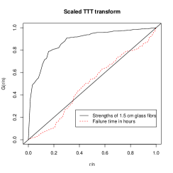
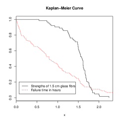
Refer to caption
Refer to caption
Figure 3: TTT plots and Kaplan-Meier curves of strengths of 1.5 cm glass fibres and the failure times in hours data.

The TTT plot and Kaplan-Meier curve for the first data in Fig. 3 shows an increasing hazard rate function and, therefore, indicates that appropriateness of the EWP distribution to fit this data. Table 1 lists the MLEs with the standard deviations of the parameters, the values of K-S (Kolmogorov-Smirnov) statistic with its respective p-value, -2log(L), AIC (Akaike Information Criterion), AD (Anderson-Darling statistic) and CM (CramΓ©r-von Mises statistic) for the first data. These values show that the EWP distribution provide a better fit than the EW, GE and Weibull for fitting the first data.

We apply the AD and CM statistics, in order to verify which distribution fits better to this data. The AD and CM test statistics are described in details in Chen and Balakrishnan [11]. In general, the smaller the values of AD and CM, the better the fit to the data. According to these statistics in Table 1, the EWP distribution fit the first data set better than the others.

Table 1: MLEs(stds.), K-S statistics, p-values, βˆ’2​log⁑(L)2𝐿-2\log(L) and AIC for the strengths of 1.5 cm glass fibres.
Dist. MLEs(stds.) K-S p-value βˆ’2​log⁑(L)2𝐿-2\log(L) AIC AD CM
EWP Ξ±^=0.578​(0.3424),Ξ²^=0.647​(0.0508)Ξ³^=5.502​(1.395),ΞΈ^=2.782​(1.568)formulae-sequence^𝛼0.5780.3424^𝛽0.6470.0508formulae-sequence^𝛾5.5021.395^πœƒ2.7821.568\begin{array}[]{l}\hat{\alpha}=0.578(0.3424),\hat{\beta}=0.647(0.0508)\\ \hat{\gamma}=5.502(1.395),\hat{\theta}=2.782(1.568)\end{array} 0.1154 0.3731 26.0 34.0 0.682 0.195
EW Ξ±^=0.671​(0.2489),Ξ²^=0.582​(0.0292)Ξ³^=7.285​(1.707)formulae-sequence^𝛼0.6710.2489^𝛽0.5820.0292^𝛾7.2851.707\begin{array}[]{l}\hat{\alpha}=0.671(0.2489),\hat{\beta}=0.582(0.0292)\\ \hat{\gamma}=7.285(1.707)\end{array} 0.1901 0.0211 29.4 35.4 1.086 0.279
GE Ξ±^^𝛼\hat{\alpha}=31.349(9.519), Ξ²^^𝛽\hat{\beta}=2.612(0.2380) 0.2291 0.0027 62.8 66.8 4.340 0.881
Weibull Ξ²^^𝛽\hat{\beta}=0.614(0.0140), Ξ³^^𝛾\hat{\gamma}=5.781(0.5761) 0.1589 0.0830 30.4 34.4 3.135 0.297

Using the likelihood ratio (LR) test, we test the null hypothesis H0: EW versus the alternative hypothesis H1: EWP, or equivalently, H0: ΞΈ=0πœƒ0\theta=0 versus H1: ΞΈβ‰ 0πœƒ0\theta\neq 0. The value of the LR test statistic and the corresponding p-value are 3.4 and 0.0651, respectively. Therefore, the null hypothesis (EW model) is rejected in favor of the alternative hypothesis (EWP model) for a significance level >> 0.0651. For test the null hypothesis H0: GE versus the alternative hypothesis H1: EWP, or equivalently, H0: (Ξ³,ΞΈ)=(1,0)π›Ύπœƒ10(\gamma,\theta)=(1,0) versus H1: (Ξ³,ΞΈ)β‰ (1,0)π›Ύπœƒ10(\gamma,\theta)\neq(1,0), the value of the LR test statistic is 36.8 (p-value = 1e-08), which includes that the null hypothesis (GE model) is rejected in favor of the alternative hypothesis (EWP model) for any significance level. We also test the null hypothesis H0: Weibull versus the alternative hypothesis H1: EWP, or equivalently, H0: (Ξ±,ΞΈ)=(1,0)π›Όπœƒ10(\alpha,\theta)=(1,0) versus H1: (Ξ±,ΞΈ)β‰ (1,0)π›Όπœƒ10(\alpha,\theta)\neq(1,0). The value of the LR test statistic is 4.4 (p-value = 0.1108), which includes that the null hypothesis (Weibull model) is rejected in favor of the alternative hypothesis (EWP model) for a significance level >> 0.1108, and for any significance level << 0.1108, the null hypothesis is not rejected but the values of AD and CM in Table 1 show that the EWP distribution gives the better fit to the first data set than the Weibull distribution.

As a second application, we consider the data show the stress-rupture life of kevlar 49/epoxy strands which were subjected to constant sustained pressure at the 90 stress level until all had failed. The failure times in hours are shown in Andrews and Herzberg [3] and Barlow et al. [4]. The TTT plot and Kaplan-Meier curve for this data in Fig. 3 shows bathtub-shaped hazard rate function and, therefore, indicates that appropriateness of the EWP distribution to fit this data. The MLEs with the standard deviations of the parameters, the values of K-S statistic, p-value, -2log(L), AIC, AD and CM are listed in Table 2. From these values, we note that the EWP model is better than the EW, GE and Weibull distributions in terms of fitting to this data.

Table 2: MLEs(stds.), K-S statistics, p-values, βˆ’2​log⁑(L)2𝐿-2\log(L) and AIC for the strengths of 1.5 cm glass fibres.
Dist. MLEs(stds.) K-S p-value βˆ’2​log⁑(L)2𝐿-2\log(L) AIC AD CM
EWP Ξ±^=0.859​(0.3681),Ξ²^=1.303​(0.7398)Ξ³^=0.8717​(0.2409),ΞΈ^=1.266​(1.2007)formulae-sequence^𝛼0.8590.3681^𝛽1.3030.7398formulae-sequence^𝛾0.87170.2409^πœƒ1.2661.2007\begin{array}[]{l}\hat{\alpha}=0.859(0.3681),\hat{\beta}=1.303(0.7398)\\ \hat{\gamma}=0.8717(0.2409),\hat{\theta}=1.266(1.2007)\end{array} 0.0725 0.6640 204.6 212.6 0.841 0.218
EW Ξ±^=0.793​(0.2870),Ξ²^=0.821​(0.2651)Ξ³^=1.060​(0.2399)formulae-sequence^𝛼0.7930.2870^𝛽0.8210.2651^𝛾1.0600.2399\begin{array}[]{l}\hat{\alpha}=0.793(0.2870),\hat{\beta}=0.821(0.2651)\\ \hat{\gamma}=1.060(0.2399)\end{array} 0.0844 0.4677 205.6 211.6 0.955 0.247
GE Ξ±^^𝛼\hat{\alpha}=0.866(0.1098), Ξ²^^𝛽\hat{\beta}=0.888(0.1201) 0.0887 0.4041 205.6 209.6 1.021 0.263
Weibull Ξ²^^𝛽\hat{\beta}=1.010(0.1141), Ξ³^^𝛾\hat{\gamma}=0.926(0.0726) 0.0907 0.3777 206.0 210.0 1.224 0.2789

Plots of the estimated pdf, cdf and survival function of the EWP, EW, GE and Weibull models fitted to the data sets corresponding to Tables 1 and 2, respectively, are given in Fig. 4. These plots suggest that the EWP distribution is superior to the EW, GE and Weibull distributions in fitting these two data sets.

14 Conclusion

A new four-parameter distribution called the EWP distribution is introduced. This distribution is a generalization of the EW distribution and contains several lifetime sub-models such as: GEP, CWP, CEP, ERP and RP. A characteristic of the EWP distribution is that its failure rate function can be decreasing, increasing, bathtub-shaped and unimodal depending on its parameter values. Several properties of the new distribution such as its probability density function, its reliability and failure rate functions, quantiles and moments is obtained. The maximum likelihood estimation procedure via a EM-algorithm is presented. Fitting the EWP model to two real data sets indicates the flexibility and capacity of the proposed distribution in data modeling. In view of the density and failure rate function shapes, it seems that the proposed model can be considered as a suitable candidate model in reliability analysis, biological systems, data modeling, and related fields.

Acknowledgement

The authors would like to sincerely thank the Editor-in-Chief, Associate Editor, and referees for carefully reading the paper and for their useful comments. The authors are also indebted to Yazd University for supporting this research.
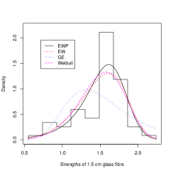
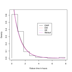
Refer to caption
Refer to caption
Refer to caption
Refer to caption
Figure 4: Fitted pdf and cdf of the EWP, EW, GE and Weibull distributions for the data sets corresponding to Tables 1 and 2, respectively.

Appendix

The elements of 4Γ—4444\times 4 observed information matrix In​(Θ)subscriptπΌπ‘›Ξ˜I_{n}\left(\Theta\right) are given by

Iα​α=βˆ’nΞ±2+ΞΈβˆ‘i=1n(1βˆ’eβˆ’(β​yi)Ξ³)Ξ±log(1βˆ’eβˆ’(Ξ²yi)Ξ³)2,
Iα​β=Ξ³β€‹βˆ‘i=1nyi​eβˆ’(β​yi)γ​(β​yi)Ξ³βˆ’11βˆ’eβˆ’(β​yi)Ξ³+ΞΈβ€‹Ξ³β€‹βˆ‘i=1nyi​eβˆ’(β​yi)γ​(1βˆ’eβˆ’(β​yi)Ξ³)Ξ±βˆ’1​(β​yi)Ξ³βˆ’1+ΞΈβ€‹Ξ±β€‹Ξ³β€‹βˆ‘i=1nyi​eβˆ’(β​yi)γ​(1βˆ’eβˆ’(β​yi)Ξ³)​logΞ±βˆ’1⁑(1βˆ’eβˆ’(β​yi)Ξ³)​(β​yi)Ξ³βˆ’1,
Iα​θ=βˆ‘i=1n(1βˆ’eβˆ’(Ξ²yi)Ξ³)​logα⁑(1βˆ’eβˆ’(Ξ²yi)Ξ³),
Iα​γ=βˆ‘i=1neβˆ’(Ξ²yi)γ​log⁑(β​yi)​(β​yi)Ξ³1βˆ’eβˆ’(β​yi)Ξ³+ΞΈβˆ‘i=1neβˆ’(β​yi)Ξ³(1βˆ’eβˆ’(β​yi)Ξ³)logΞ±βˆ’1(Ξ²yi)(Ξ²yi)Ξ³+Ξ±β€‹ΞΈβ€‹βˆ‘i=1neβˆ’(β​yi)γ​(1βˆ’eβˆ’(β​yi)Ξ³)Ξ±βˆ’1​log⁑(1βˆ’eβˆ’(β​yi)Ξ³)​log⁑(β​yi)​(β​yi)Ξ³,
Iβ​β=βˆ’nΞ²2βˆ’Ξ³(Ξ³βˆ’1)βˆ‘i=1nyi2(Ξ²yi)+Ξ³βˆ’2(Ξ±βˆ’1)Ξ³(Ξ³βˆ’1)βˆ‘i=1nyi2eβˆ’(Ξ²yi)Ξ³(Ξ²yi)Ξ³βˆ’21βˆ’eβˆ’(Ξ²yi)Ξ³βˆ’(Ξ±βˆ’1)​γ2β€‹βˆ‘i=1nyi2​eβˆ’2(Ξ²yi)Ξ³(Ξ²yi)2​(Ξ³βˆ’1)(1βˆ’eβˆ’(Ξ²yi)Ξ³)2βˆ’(Ξ±βˆ’1)​γ2β€‹βˆ‘i=1nyi2​eβˆ’(Ξ²yi)Ξ³(Ξ²yi)2​(Ξ³βˆ’1)1βˆ’eβˆ’(Ξ²yi)Ξ³+Ξ±ΞΈΞ³(Ξ³βˆ’1)βˆ‘i=1nyi2eβˆ’(Ξ²yi)Ξ³(1βˆ’eβˆ’(Ξ²yi)Ξ³)(Ξ²yi)Ξ±βˆ’1Ξ³βˆ’2βˆ’Ξ±ΞΈΞ³2βˆ‘i=1nyi2eβˆ’(Ξ²yi)Ξ³(1βˆ’eβˆ’(Ξ²yi)Ξ³)(Ξ²yi)Ξ±βˆ’12​(Ξ³βˆ’1)+Ξ±(Ξ±βˆ’1)ΞΈΞ³2βˆ‘i=1nyi2eβˆ’2(Ξ²yi)Ξ³(1βˆ’eβˆ’(Ξ²yi)Ξ³)(Ξ²yi)Ξ±βˆ’2,2​(Ξ³βˆ’1)
Iβ​θ=Ξ±Ξ³βˆ‘i=1nyieβˆ’(Ξ²yi)Ξ³(1βˆ’eβˆ’(Ξ²yi)Ξ³)(Ξ²yi)Ξ±βˆ’1,Ξ³βˆ’1
Iβ​γ=βˆ’βˆ‘i=1nyi(Ξ²yi)βˆ’Ξ³βˆ’1Ξ³βˆ‘i=1nyilog(Ξ²yi)(Ξ²yi)+Ξ³βˆ’1(Ξ±βˆ’1)βˆ‘i=1nyieβˆ’(Ξ²yi)Ξ³(Ξ²yi)Ξ³βˆ’11βˆ’eβˆ’(β​yi)Ξ³+(Ξ±βˆ’1)β€‹Ξ³β€‹βˆ‘i=1nyi​eβˆ’(Ξ²yi)Ξ³log(Ξ²yi)(Ξ²yi)Ξ³βˆ’11βˆ’eβˆ’(Ξ²yi)Ξ³βˆ’(Ξ±βˆ’1)β€‹Ξ³β€‹βˆ‘i=1nyi​eβˆ’2(Ξ²yi)Ξ³log(Ξ²yi)(Ξ²yi)2β€‹Ξ³βˆ’1(1βˆ’eβˆ’(Ξ²yi)Ξ³)2βˆ’(Ξ±βˆ’1)Ξ³βˆ‘i=1nyieβˆ’(Ξ²yi)Ξ³log(Ξ²yi)(Ξ²yi)2β€‹Ξ³βˆ’11βˆ’eβˆ’(Ξ²yi)Ξ³+Ξ±ΞΈβˆ‘i=1nyieβˆ’(Ξ²yi)Ξ³(1βˆ’eβˆ’(Ξ²yi)Ξ³)(Ξ²yi)Ξ±βˆ’1Ξ³βˆ’1+Ξ±ΞΈΞ³βˆ‘i=1nyieβˆ’(Ξ²yi)Ξ³(1βˆ’eβˆ’(Ξ²yi)Ξ³)logΞ±βˆ’1(Ξ²yi)(Ξ²yi)Ξ³βˆ’1βˆ’Ξ±ΞΈΞ³βˆ‘i=1nyieβˆ’(Ξ²yi)Ξ³(1βˆ’eβˆ’(Ξ²yi)Ξ³)logΞ±βˆ’1(Ξ²yi)(Ξ²yi)2β€‹Ξ³βˆ’1+Ξ±(Ξ±βˆ’1)ΞΈΞ³βˆ‘i=1nyieβˆ’2(Ξ²yi)Ξ³(1βˆ’eβˆ’(Ξ²yi)Ξ³)logΞ±βˆ’2(Ξ²yi)(Ξ²yi),2β€‹Ξ³βˆ’1
\begin{array}[]{ll}I_{\alpha\alpha}&=-\frac{n}{\alpha^{2}}+\theta\sum_{i=1}^{n}\left(1-e^{-\left(\beta y_{i}\right)^{\gamma}}\right)^{\alpha}\log\left(1-e^{-\left(\beta y_{i}\right){}^{\gamma}}\right)^{2},\vskip 12.0pt plus 4.0pt minus 4.0pt\\ I_{\alpha\beta}&=\gamma\sum_{i=1}^{n}y_{i}\frac{e^{-\left(\beta y_{i}\right)^{\gamma}}\left(\beta y_{i}\right)^{\gamma-1}}{1-e^{-\left(\beta y_{i}\right)^{\gamma}}}+\theta\gamma\sum_{i=1}^{n}y_{i}e^{-\left(\beta y_{i}\right)^{\gamma}}\left(1-e^{-\left(\beta y_{i}\right)^{\gamma}}\right)^{\alpha-1}\left(\beta y_{i}\right)^{\gamma-1}\vskip 6.0pt plus 2.0pt minus 2.0pt\\ &~{}~{}+\theta\alpha\gamma\sum_{i=1}^{n}y_{i}e^{-\left(\beta y_{i}\right)^{\gamma}}\left(1-e^{-\left(\beta y_{i}\right)^{\gamma}}\right){}^{\alpha-1}\log\left(1-e^{-\left(\beta y_{i}\right)^{\gamma}}\right)\left(\beta y_{i}\right)^{\gamma-1},\vskip 12.0pt plus 4.0pt minus 4.0pt\\ I_{\alpha\theta}&=\sum_{i=1}^{n}\left(1-e^{-\left(\beta y_{i}\right){}^{\gamma}}\right){}^{\alpha}\log\left(1-e^{-\left(\beta y_{i}\right){}^{\gamma}}\right),\vskip 12.0pt plus 4.0pt minus 4.0pt\\ I_{\alpha\gamma}&=\sum_{i=1}^{n}\frac{e^{-\left(\beta y_{i}\right){}^{\gamma}}\log\left(\beta y_{i}\right)\left(\beta y_{i}\right)^{\gamma}}{1-e^{-\left(\beta y_{i}\right)^{\gamma}}}+\theta\sum_{i=1}^{n}e^{-\left(\beta y_{i}\right)^{\gamma}}\left(1-e^{-\left(\beta y_{i}\right)^{\gamma}}\right){}^{\alpha-1}\log\left(\beta y_{i}\right)\left(\beta y_{i}\right){}^{\gamma}\vskip 6.0pt plus 2.0pt minus 2.0pt\\ &~{}~{}+\alpha\theta\sum_{i=1}^{n}e^{-\left(\beta y_{i}\right)^{\gamma}}\left(1-e^{-\left(\beta y_{i}\right)^{\gamma}}\right)^{\alpha-1}\log\left(1-e^{-\left(\beta y_{i}\right)^{\gamma}}\right)\log\left(\beta y_{i}\right)\left(\beta y_{i}\right)^{\gamma},\vskip 12.0pt plus 4.0pt minus 4.0pt\\ I_{\beta\beta}&=-\frac{n}{\beta^{2}}-\gamma(\gamma-1)\sum_{i=1}^{n}y_{i}^{2}\left(\beta y_{i}\right){}^{\gamma-2}+(\alpha-1)\gamma(\gamma-1)\sum_{i=1}^{n}y_{i}^{2}\frac{e^{-\left(\beta y_{i}\right){}^{\gamma}}\left(\beta y_{i}\right){}^{\gamma-2}}{1-e^{-\left(\beta y_{i}\right){}^{\gamma}}}\vskip 6.0pt plus 2.0pt minus 2.0pt\\ &~{}~{}-(\alpha-1)\gamma^{2}\sum_{i=1}^{n}y_{i}^{2}\frac{e^{-2\left(\beta y_{i}\right){}^{\gamma}}\left(\beta y_{i}\right){}^{2(\gamma-1)}}{\left(1-e^{-\left(\beta y_{i}\right){}^{\gamma}}\right){}^{2}}-(\alpha-1)\gamma^{2}\sum_{i=1}^{n}y_{i}^{2}\frac{e^{-\left(\beta y_{i}\right){}^{\gamma}}\left(\beta y_{i}\right){}^{2(\gamma-1)}}{1-e^{-\left(\beta y_{i}\right){}^{\gamma}}}\vskip 6.0pt plus 2.0pt minus 2.0pt\\ &~{}~{}+\alpha\theta\gamma(\gamma-1)\sum_{i=1}^{n}y_{i}^{2}e^{-\left(\beta y_{i}\right){}^{\gamma}}\left(1-e^{-\left(\beta y_{i}\right){}^{\gamma}}\right){}^{\alpha-1}\left(\beta y_{i}\right){}^{\gamma-2}\vskip 6.0pt plus 2.0pt minus 2.0pt\\ &~{}~{}-\alpha\theta\gamma^{2}\sum_{i=1}^{n}y_{i}^{2}e^{-\left(\beta y_{i}\right){}^{\gamma}}\left(1-e^{-\left(\beta y_{i}\right){}^{\gamma}}\right){}^{\alpha-1}\left(\beta y_{i}\right){}^{2(\gamma-1)}\vskip 6.0pt plus 2.0pt minus 2.0pt\\ &~{}~{}+\alpha(\alpha-1)\theta\gamma^{2}\sum_{i=1}^{n}y_{i}^{2}e^{-2\left(\beta y_{i}\right){}^{\gamma}}\left(1-e^{-\left(\beta y_{i}\right){}^{\gamma}}\right){}^{\alpha-2}\left(\beta y_{i}\right){}^{2(\gamma-1)},\vskip 12.0pt plus 4.0pt minus 4.0pt\\ I_{\beta\theta}&=\alpha\gamma\sum_{i=1}^{n}y_{i}e^{-\left(\beta y_{i}\right){}^{\gamma}}\left(1-e^{-\left(\beta y_{i}\right){}^{\gamma}}\right){}^{\alpha-1}\left(\beta y_{i}\right){}^{\gamma-1},\vskip 12.0pt plus 4.0pt minus 4.0pt\\ I_{\beta\gamma}&=-\sum_{i=1}^{n}y_{i}\left(\beta y_{i}\right){}^{\gamma-1}-\gamma\sum_{i=1}^{n}y_{i}\log\left(\beta y_{i}\right)\left(\beta y_{i}\right){}^{\gamma-1}+(\alpha-1)\sum_{i=1}^{n}y_{i}\frac{e^{-\left(\beta y_{i}\right){}^{\gamma}}\left(\beta y_{i}\right){}^{\gamma-1}}{1-e^{-\left(\beta y_{i}\right)^{\gamma}}}\vskip 6.0pt plus 2.0pt minus 2.0pt\\ &~{}~{}+(\alpha-1)\gamma\sum_{i=1}^{n}y_{i}\frac{e^{-\left(\beta y_{i}\right){}^{\gamma}}\log\left(\beta y_{i}\right)\left(\beta y_{i}\right){}^{\gamma-1}}{1-e^{-\left(\beta y_{i}\right){}^{\gamma}}}-(\alpha-1)\gamma\sum_{i=1}^{n}y_{i}\frac{e^{-2\left(\beta y_{i}\right){}^{\gamma}}\log\left(\beta y_{i}\right)\left(\beta y_{i}\right){}^{2\gamma-1}}{\left(1-e^{-\left(\beta y_{i}\right){}^{\gamma}}\right){}^{2}}\vskip 6.0pt plus 2.0pt minus 2.0pt\\ &~{}~{}-(\alpha-1)\gamma\sum_{i=1}^{n}y_{i}\frac{e^{-\left(\beta y_{i}\right){}^{\gamma}}\log\left(\beta y_{i}\right)\left(\beta y_{i}\right){}^{2\gamma-1}}{1-e^{-\left(\beta y_{i}\right){}^{\gamma}}}+\alpha\theta\sum_{i=1}^{n}y_{i}e^{-\left(\beta y_{i}\right){}^{\gamma}}\left(1-e^{-\left(\beta y_{i}\right){}^{\gamma}}\right){}^{\alpha-1}\left(\beta y_{i}\right){}^{\gamma-1}\vskip 6.0pt plus 2.0pt minus 2.0pt\\ &~{}~{}+\alpha\theta\gamma\sum_{i=1}^{n}y_{i}e^{-\left(\beta y_{i}\right){}^{\gamma}}\left(1-e^{-\left(\beta y_{i}\right){}^{\gamma}}\right){}^{\alpha-1}\log\left(\beta y_{i}\right)\left(\beta y_{i}\right){}^{\gamma-1}\vskip 6.0pt plus 2.0pt minus 2.0pt\\ &~{}~{}-\alpha\theta\gamma\sum_{i=1}^{n}y_{i}e^{-\left(\beta y_{i}\right){}^{\gamma}}\left(1-e^{-\left(\beta y_{i}\right){}^{\gamma}}\right){}^{\alpha-1}\log\left(\beta y_{i}\right)\left(\beta y_{i}\right){}^{2\gamma-1}\vskip 6.0pt plus 2.0pt minus 2.0pt\\ &~{}~{}+\alpha(\alpha-1)\theta\gamma\sum_{i=1}^{n}y_{i}e^{-2\left(\beta y_{i}\right){}^{\gamma}}\left(1-e^{-\left(\beta y_{i}\right){}^{\gamma}}\right){}^{\alpha-2}\log\left(\beta y_{i}\right)\left(\beta y_{i}\right){}^{2\gamma-1},\end{array}
Iθ​θ=n​eβˆ’ΞΈ(eβˆ’ΞΈβˆ’1)2βˆ’nΞΈ2,
Iθ​γ=Ξ±βˆ‘i=1neβˆ’(Ξ²yi)Ξ³(1βˆ’eβˆ’(Ξ²yi)Ξ³)logΞ±βˆ’1(Ξ²yi)(Ξ²yi),Ξ³
Iγ​γ=βˆ’nΞ³2βˆ’βˆ‘i=1nlog(Ξ²yi)2(Ξ²yi)Ξ³+(Ξ±βˆ’1)βˆ‘i=1neβˆ’(Ξ²yi)Ξ³log(Ξ²yi)2(Ξ²yi)Ξ³1βˆ’eβˆ’(β​yi)Ξ³βˆ’(Ξ±βˆ’1)β€‹βˆ‘i=1neβˆ’2(Ξ²yi)Ξ³log(Ξ²yi)2(Ξ²yi)2​γ(1βˆ’eβˆ’(Ξ²yi)Ξ³)2βˆ’(Ξ±βˆ’1)β€‹βˆ‘i=1neβˆ’(β​yi)Ξ³log(Ξ²yi)2(Ξ²yi)2​γ1βˆ’eβˆ’(β​yi)Ξ³+Ξ±ΞΈβˆ‘i=1neβˆ’(β​yi)Ξ³(1βˆ’eβˆ’(β​yi)Ξ³)Ξ±βˆ’1log(Ξ²yi)2(Ξ²yi)Ξ³βˆ’Ξ±ΞΈβˆ‘i=1neβˆ’(β​yi)Ξ³(1βˆ’eβˆ’(β​yi)Ξ³)Ξ±βˆ’1log(Ξ²yi)2(Ξ²yi)2​γ+Ξ±(Ξ±βˆ’1)ΞΈβˆ‘i=1neβˆ’2​(β​yi)Ξ³(1βˆ’eβˆ’(Ξ²yi)Ξ³)Ξ±βˆ’2log(Ξ²yi)2(Ξ²yi)2​γ.
\begin{array}[]{ll}I_{\theta\theta}&=\frac{ne^{-\theta}}{\left(e^{-\theta}-1\right)^{2}}-\frac{n}{\theta^{2}},\vskip 12.0pt plus 4.0pt minus 4.0pt\\ I_{\theta\gamma}&=\alpha\sum_{i=1}^{n}e^{-\left(\beta y_{i}\right){}^{\gamma}}\left(1-e^{-\left(\beta y_{i}\right){}^{\gamma}}\right){}^{\alpha-1}\log\left(\beta y_{i}\right)\left(\beta y_{i}\right){}^{\gamma},\vskip 12.0pt plus 4.0pt minus 4.0pt\\ I_{\gamma\gamma}&=-\frac{n}{\gamma^{2}}-\sum_{i=1}^{n}\log\left(\beta y_{i}\right)^{2}\left(\beta y_{i}\right)^{\gamma}+(\alpha-1)\sum_{i=1}^{n}\frac{e^{-\left(\beta y_{i}\right){}^{\gamma}}\log\left(\beta y_{i}\right)^{2}\left(\beta y_{i}\right)^{\gamma}}{1-e^{-\left(\beta y_{i}\right)^{\gamma}}}\vskip 6.0pt plus 2.0pt minus 2.0pt\\ &~{}~{}-(\alpha-1)\sum_{i=1}^{n}\frac{e^{-2\left(\beta y_{i}\right){}^{\gamma}}\log\left(\beta y_{i}\right)^{2}\left(\beta y_{i}\right)^{2\gamma}}{\left(1-e^{-\left(\beta y_{i}\right){}^{\gamma}}\right){}^{2}}-(\alpha-1)\sum_{i=1}^{n}\frac{e^{-\left(\beta y_{i}\right)^{\gamma}}\log\left(\beta y_{i}\right)^{2}\left(\beta y_{i}\right){}^{2\gamma}}{1-e^{-\left(\beta y_{i}\right)^{\gamma}}}\vskip 6.0pt plus 2.0pt minus 2.0pt\\ &~{}~{}+\alpha\theta\sum_{i=1}^{n}e^{-\left(\beta y_{i}\right)^{\gamma}}\left(1-e^{-\left(\beta y_{i}\right)^{\gamma}}\right)^{\alpha-1}\log\left(\beta y_{i}\right)^{2}\left(\beta y_{i}\right){}^{\gamma}\vskip 6.0pt plus 2.0pt minus 2.0pt\\ &~{}~{}-\alpha\theta\sum_{i=1}^{n}e^{-\left(\beta y_{i}\right)^{\gamma}}\left(1-e^{-\left(\beta y_{i}\right)^{\gamma}}\right)^{\alpha-1}\log\left(\beta y_{i}\right)^{2}\left(\beta y_{i}\right)^{2\gamma}\vskip 6.0pt plus 2.0pt minus 2.0pt\\ &~{}~{}+\alpha(\alpha-1)\theta\sum_{i=1}^{n}e^{-2\left(\beta y_{i}\right)^{\gamma}}\left(1-e^{-\left(\beta y_{i}\right){}^{\gamma}}\right)^{\alpha-2}\log\left(\beta y_{i}\right)^{2}\left(\beta y_{i}\right)^{2\gamma}.\end{array}

References

  • [1] M.V. Aarset, How to identify bathtub hazard rate, IEEE Transactions Reliability 36 (1987) 106-108.
  • [2] K. Adamidis, S. Loukas, A lifetime distribution with decreasing failure rate, Statistics and Probability Letters 39 (1998) 35-42.
  • [3] D.F. Andrews, A.M. Herzberg, Data: A Collection of Problems from Many Fields for the Student and Research Worker, Springer Series in Statistics, New York, 1985.
  • [4] R.E. Barlow, R.H. Toland, T. Freeman, A Bayesian analysis of stress-rupture life of kevlar 49/epoxy spherical pressure vessels, In: Proceeding of Canadian Conference in Applied Statistics, Marcel Dekker, New York, 1984.
  • [5] W. Barreto-Souza, F. Cribari-Neto, A generalization of the exponential-Poisson distribution, Statistics and Probability Letters 79 (2009) 2493-2500.
  • [6] W. Barreto-Souza, A.H.S., Santos, G.M. Cordeiro, The beta generalized exponential distribution, Journal of Statistical Computation and Simulation 80 (2010) 159-172.
  • [7] W. Barreto-Souza, A.L. Morais, G.M. Cordeiro, The Weibull-geometric distribution, Journal of Statistical Computation and Simulation 81 (2011) 645-657.
  • [8] A. Basu, J. Klein, Some recent development in competing risks theory, In: J. Crowley, R.A. Johnson(Eds.), Survival Analysis, IMS, Hayward, 1982, pp. 216-229.
  • [9] V.G. Cancho, F. Louzada-Neto, G.D.C. Barriga, The Poisson-exponential lifetime distribution, Computational Statistics and Data Analysis 55 (2011) 677-686.
  • [10] M. Chahkandi, M. Ganjali, On some lifetime distributions with decreasing failure rate, Computational Statistics and Data Analysis 53 (2009) 4433-4440.
  • [11] G. Chen, N. Balakrishnan, A general purpose approximate goodness-of-fit test, Journal of Quality Technology 27 (1995) 154-161.
  • [12] A. Choudhury, A Simple derivation of moments of the exponentiated Weibull distribution, Metrika 62 (2005) 17-22.
  • [13] A.P. Dempster, N.M. Laird, D.B. Rubin, Maximum likelihood from incomplete data via the EM algorithm (with discussion), Journal of Royal Statistical Socity Ser. B 39 (1977) 1-38.
  • [14] M.E. Ghitany, On a recent generalization of gamma distribution, Communications in Statistics-Theory and Methods 27 (1998) 223-233.
  • [15] G.M. Giorgi, Concentration index, Bonferroni. Encyclopedia of Statistical Sciences, vol. 2, Wiley, New York, 1998, pp. 141-146.
  • [16] G.M. Giorgi, M. Crescenzi, A look at the Bonferroni inequality measure in a reliability framework. Statistica LXL 4 (2001) 571-583.
  • [17] J.A. Greenwood, J.M. Landwehr, N.C. Matalas, J.R. Wallis, Probability weighted moments: Definition and relation to parameters of several distribution exprensible in inverse form, Water Resources Research 15 (1979) 1049-1054.
  • [18] P.L. Gupta, R.C. Gupta, On the moments of residual life in reliability and some characterization results, Communications in Statistics-Theory and Methods 12 (1983) 449-461.
  • [19] R.D. Gupta, D. Kundu, Exponentiated exponential family: an alternative to gamma and Weibull distributions, Biometrika Journal 43 (2001) 117-130.
  • [20] J.R.M. Hosking, J.R. Wallis, E.F. Wood, Estimation of the generalized extreme value distribution by the method of probability weighted moments, Technometrics 27 (1985) 251-261.
  • [21] J.R.M. Hosking, The Theory of Probability Weighted Moments, IBM Research Report. RC 12210, Yorktown Heights, NY., 1986.
  • [22] C. Kundu, A.K. Nanda, Some reliability properties of the inactivity time, Communications in Statistics-Theory and Methods 39 (2010) 899-911.
  • [23] C. Kus, A new lifetime distribution, Computational Statistics and Data Analysis 51 (2007) 4497-4509.
  • [24] F. Louzada, M. Roman, V.G. Cancho, The complementary exponential geometric distribution: model, properties, and comparison with its counter part, Computational Statistics and Data Analysis 55 (2011) 2516-2524.
  • [25] E. Mahmoudi, A.A. Jafari, Generalized exponential-power series distributions, Computational Statistics and Data Analysis 56 (2012) 4047-4066.
  • [26] E. Mahmoudi, A. Sepahdar, Exponentiated Weibull-logarithmic distribution, submitted for publication.
  • [27] E. Mahmoudi, M. Shiran, Exponentiated Weibull-geometric distribution and its applications, submitted for publication, http://arxiv.org/abs/1206.4008v1.
  • [28] E. Mahmoudi, M. Shiran, Exponentiated Weibull-power series distribution, submitted for publication.
  • [29] G.J. McLachlan and T. Krishnan, The EM Algorithm and Extension,Wiley, NewYork, 1997.
  • [30] J. Mi, Bathtub failure rate and upside-down bathtub mean residual life, IEEE Transactions on Reliability 44 (1995) 388-391.
  • [31] A.L. Morais, W. Barreto-Souza, A compound class of Weibull and power series distributions, Computational Statistics and Data Analysis 55 (2011) 1410-1425.
  • [32] G.S. Mudholkar, D.K. Srivastava, Exponentiated Weibull family for analyzing bathtub failure-rate data, IEEE Transactions on Reliability 42 (1993) 299-302.
  • [33] G.S. Mudholkar, D.K. Srivastava, M. Freimer, The exponentiated Weibull family: a reanalysis of the bus-motor-failure data, Technometrics 37 (1995) 436-445.
  • [34] G.S. Mudholkar, A.D. Hustson, The exponentiated Weibull family: some properties and a flood data application, Communications in Statistics-Theory and Methods 25 (1996) 3059-3083.
  • [35] A.K. Nanda, H. Singh, N. Misra, P. Paul, Reliability properties of reversed residual lifetime, Communications in Statistics-Theory and Methods 32 (2003) 2031-2042.
  • [36] M.M. Nassar, F.H. Eissa, On the exponentiated Weibull distribution, Communications in Statistics-Theory and Methods 32 (2003) 1317-1336.
  • [37] K.S. Park, Effect of burn-in on mean residual life, IEEE Transactions on Reliability 34 (1985) 522-523.
  • [38] R. Tahmasbi S. Rezaei, A two-parameter lifetime distribution with decreasing failure rate, Computational Statistics and Data Analysis 52 (2008) 3889-3901.
  • [39] L.C. Tang, Y. Lu, E.P. Chew, Mean residual life distributions, IEEE Transactions on Reliability 48 (1999) 68-73.