The random subgraph model for the analysis of an ecclesiastical network in Merovingian Gaul

Abstract

In the last two decades many random graph models have been proposed to extract knowledge from networks. Most of them look for communities or, more generally, clusters of vertices with homogeneous connection profiles. While the first models focused on networks with binary edges only, extensions now allow to deal with valued networks. Recently, new models were also introduced in order to characterize connection patterns in networks through mixed memberships. This work was motivated by the need of analyzing a historical network where a partition of the vertices is given and where edges are typed. A known partition is seen as a decomposition of a network into subgraphs that we propose to model using a stochastic model with unknown latent clusters. Each subgraph has its own mixing vector and sees its vertices associated to the clusters. The vertices then connect with a probability depending on the subgraphs only, while the types of edges are assumed to be sampled from the latent clusters. A variational Bayes expectation-maximization algorithm is proposed for inference as well as a model selection criterion for the estimation of the cluster number. Experiments are carried out on simulated data to assess the approach. The proposed methodology is then applied to an ecclesiastical network in Merovingian Gaul. An R code, called Rambo, implementing the inference algorithm is available from the authors upon request.

, , , , and

1 Introduction

Since the original work of Moreno (1934) on sociograms, network data has become ubiquitous in Biology [Albert and Barabási (2002), Milo et al. (2002), Palla et al. (2005)] and computational social sciences [Snijders and Nowicki (1997)]. Applications range from the study of gene regulation processes to that of social interactions. Network analysis was also applied recently to a medieval social network in Villa, Rossi and Truong (2008), where the authors find a clustering of vertices through kernel methods. Both deterministic and probabilistic methods have been used to seek structure in these networks, depending on prior knowledge and assumptions on the form of the data. For example, Hofman and Wiggins (2008) looked for a partition of the vertices where the clusters exhibit a transitivity property. The model of Handcock, Raftery and Tantrum (2007), on the other hand, assumes the relations to be conditioned on the projection of the vertices in a latent social space. Notable among the community discovery methods, though asymptotically biased [Bickel and Chen (2009)], are those based on the modularity score given by Girvan and Newman (2002).

Many of the other currently used methods derive from the stochastic block model (SBM) [Wang and Wong (1987), Nowicki and Snijders (2001)], which is a probabilistic generalization [Fienberg and Wasserman (1981)] of the method applied by White, Boorman and Breiger (1976) to Sampson’s famous monastery data. SBM assumes that each vertex belongs to a hidden cluster and that connection probabilities between a pair of vertices depend exclusively on their clusters, as in Frank and Harary (1982). The parameters and clusters are then inferred to optimize a criterion, usually a lower bound of an integrated log-likelihood. Thus, Latouche, Birmelé and Ambroise (2011) used an approximation of the marginal log-likelihood, while Daudin, Picard and Robin (2008) considered a Laplace approximation of the integrated classification log-likelihood. A nonparametric Bayesian approach was also introduced by Kemp et al. (2006) to estimate the number of clusters while clustering the vertices. SBM was extended by the mixed membership stochastic block model (MMSBM) [Airoldi et al. (2008)], which allows a vertex to belong to different clusters in its relations toward different vertices, and by the overlapping stochastic block model (OSBM) [Latouche, Birmelé and Ambroise (2011)], which allows a vertex to belong to no cluster or to several at the same time. More recent works focused on extending MMSBM to dynamic networks [Xing, Fu and Song (2010)] or dealing with nonbinary networks, such as networks with weighted edges [Soufiani and Airoldi (2012)]. Goldenberg, Zheng and Fienberg (2010) and Salter-Townshend et al. (2012) provide extensive reviews of statistical network models.

In this paper we aim at clustering the vertices of networks with typed edges and for which a partition of the nodes into subgraphs is observed and bears some importance in their behavior. For example, one may be interested in looking for latent clusters in a worldwide social network describing social interactions between individuals where different countries, or at a different scale, different regions of the world, have different connectivity patterns. We might also observe the same kind of phenomenon between different scientific fields in a citation network. This kind of network may be modelled using generalized linear models [Fienberg and Wasserman (1981)] by incorporating the observed partition information as covariates and the clusters serving as random effects or a $p1$ model [Holland and Leinhardt (1981)], where the clusters allow for the estimation of interactions. However, we consider here a different strategy and propose an extension of the SBM model which has the advantage of relying on easy to interpret parameters. Indeed, SBM parameters are not expressed through nonlinear functions like the log or logistic functions and this allows an easy interpretation for nonstatisticians.

This point is of crucial interest in this work because we aim at providing historians with insight into the relationships between ecclesiastics and notable people in the kingdoms that made up Merovingian Gaul, by analyzing a network characterizing their different kinds of relations. Specifically, the data set focuses on the relationships between individuals built during the ecclesiastical councils which took place in Gaul during the 6th century. These councils were convened under the authority of a bishop to discuss specific questions relating to the Church. Though consisting mainly of clergymen, laics would also occasionally take part, as representatives of the secular power or experts in the questions discussed. These assemblies shaped a significant part of that period, and we are interested in discovering how they reflected the relationships between various groups of individuals. For this network, extra information on the vertices, namely, a geographical partition, is available, associating each individual to a specific kingdom. This partition induces a decomposition of the network into subgraphs and we aim at modelling the connection pattern of each subgraph through latent clusters.

Thus, in this paper, we propose a new model, that we call the random subgraph model (RSM), for the analysis of directed networks with typed edges for which a partition of the vertices is available. On the one hand, we consider that the probability of observing an edge between two vertices depends solely on the subgraphs to which the vertices belong. On the other hand, we assume that each vertex belongs to a hidden cluster, with a probability depending on its subgraph. Then, if a relation is present, its type is drawn from a multinomial distribution whose parameters depend on the clusters to which the vertices belong. Let us emphasize that the latter property allows, once the inference is done, to compare the different subgraphs.

The choice of proposing a probabilistic rather than a deterministic model is again motivated by the nature of the historical network we consider. Indeed, as mentioned in Section 4, the data set was built from a collection of data at hand using sources such as council acts or narrative texts. However, the rarity of the sources only allowed an incomplete or approximate characterization of the relations between individuals. Therefore, we rely on the probabilistic framework in order to deal with the uncertainty on the edges. Moreover, we emphasize that probabilistic methods for network analysis are appealing in general because they have been shown to be flexible and capable of retrieving complex heterogeneous structures in networks [see, for instance, Airoldi et al. (2008), Goldenberg, Zheng and Fienberg (2010)].

The article is organized as follows. The random subgraph model is presented along with its inference algorithm in Section 2, then tested on simulated data and compared to other models in Section 3. Our model is then applied to the ecclesiastical network and the results are analyzed from the historical point of view in Section 4. Concluding remarks and possible extensions are finally discussed in Section 5.

2 The random subgraph model

We consider a directed graph $\mathcal{G}$ with $N$ vertices represented by its $N\times N$ adjacency matrix $\mathbf{X}$ along with a known partition $\mathcal{P}$ of the vertices into $S$ classes. Our goal is to cluster the network into $K$ groups with homogeneous connection profiles, that is, estimating a binary matrix $\mathbf{Z}$ such that $Z_{ik}=1$ if vertex $i$ belongs to cluster $k$, $0$ otherwise.

Let us now detail the notation. Each edge $X_{ij}$, describing the relation between the vertices $i$ and $j$, is typed, that is, takes its values in a finite set $\{0,\ldots,C\}$. Note that $X_{ij}=0$ corresponds to the absence of an edge. We assume that $\mathcal{G}$ does not have any self loop and, therefore, the entries $X_{ii}$ will not be taken into account. In order to simplify the notation when describing the model, we also consider the binary matrix $\mathbf{A}$ with entries $A_{ij}$ such that $A_{i,j}=1\iff X_{i,j}\neq 0$.

We also emphasize that the observed partition $\mathcal{P}$ induces a decomposition of the graph into subgraphs where each class of vertices corresponds to a specific subgraph. We introduce the variable $s_{i}$ which takes its values in $\{1,\ldots,S\}$ and is used to indicate in which of the subgraphs vertex $i$ belongs, for $i\in\{1,\ldots,N\}$.

2.1 The probabilistic model

The data is assumed to be generated in three steps. First, the presence of an edge from vertex $i$ to vertex $j$ is supposed to follow a Bernouilli distribution whose parameter depends on the subgraphs $s_{i}$ and $s_{j}$ only:

$$A_{i,j}\sim\mathcal{B}(\gamma_{s_{i},s_{j}}).$$

Each vertex $i$ is then associated to a latent cluster with a probability depending on $s_{i}$. In practice, if we assume for now that the number $K$ of latent clusters is known, the variable $\mathbf{Z}_{i}$ is drawn from a multinomial distribution:

$$\mathbf{Z}_{i}\sim\mathcal{M}(1;\bolds\alpha_{s_{i}}),$$

where

$$\forall s\in{1,\ldots,S}\qquad\sum_{k=1}^{K}{\alpha_{sk}}=1.$$

A notable point of the model is that we allow each subgraph to have different mixing proportions $\bolds{\alpha}_{s}$ for the latent clusters. We denote hereafter $\bolds{\alpha}=(\bolds{\alpha}_{1},\ldots,\bolds{\alpha}_{S})$. Finally, if an edge between $i$ and $j$ is present, that is, $A_{ij}=1$, its type $X_{ij}$ is sampled from a multinomial distribution with parameters depending on the latent clusters. Thus, if $i$ belongs to cluster $k$ and $j$ to cluster $l$,

$$X_{i,j}|Z_{ik}Z_{jl}=1,\qquad A_{ij}=1\sim\mathcal{M}(1,\bolds\Pi_{kl}),$$

where the sum over the $C$ types of each vector $\bolds\Pi_{kl}=(\Pi_{kl1},\ldots,\Pi_{klC})$ is

$$\forall(k,l)\in\{1,\ldots,K\}^{2}\qquad\sum_{c=1}^{C}{\Pi_{klc}}=1.$$

If there is no edge between the two vertices, the entry $X_{ij}$ is simply set to $X_{ij}=A_{ij}=0$.

The model is therefore defined through the joint distribution

$$p(\mathbf{X},\mathbf{A},\mathbf{Z}|\bolds{\alpha},\bolds{\gamma},\bolds{\Pi}) = p(\mathbf{X},\mathbf{A}|\mathbf{Z},\bolds{\gamma},\bolds{\Pi})p(\mathbf{Z}|\bolds{\alpha})$$

$$= p(\mathbf{X}|\mathbf{A},\mathbf{Z},\bolds{\Pi})p(\mathbf{A}|\bolds{\gamma})p(\mathbf{Z}|\bolds{\alpha}),$$

where

$$p(\mathbf{X}|\mathbf{A},\mathbf{Z},\bolds{\Pi})=\prod_{k,l}^{K}\prod_{c=1}^{C}\bigl{(}\Pi_{kl}^{c}\bigr{)}^{\sum_{i\neq j}^{N}\delta(X_{ij}=c)A_{ij}Z_{ik}Z_{jl}}$$

and

$$p(\mathbf{A}|\bolds{\gamma})=\prod_{i\neq j}^{N}\gamma_{r_{i},r_{j}}^{A_{ij}}(1-\gamma_{r_{i},r_{j}})^{1-A_{ij}}.$$

Finally,

$$p(\mathbf{Z}|\bolds{\alpha})=\prod_{i=1}^{N}\prod_{k=1}^{K}\alpha_{r_{i},k}^{Z_{ik}}.$$

We refer to the Appendix for the detailed calculation of the complete data log-likelihood associated to the RSM model and summarize the model parameters in Table 1.

Table 1: Summary of the notation used in the paper

Notation	Description
$\mathbf{X}$	Adjacency matrix. $X_{ij}\in\{0,\ldots,C\}$ indicates the edge type
$\mathbf{A}$	Binary matrix. $A_{ij}=1$ indicates the presence of an edge
$\mathbf{Z}$	Binary matrix. $Z_{ik}=1$ indicates that $i$ belongs to cluster $k$
$N$	Number of vertices in the network
$K$	Number of latent clusters
$S$	Number of subgraphs
$C$	Number of edge types
$\bolds{\alpha}$	$\alpha_{sk}$ is the proportion of cluster $k$ in subgraph $s$
$\bolds{\Pi}$	$\Pi_{klc}$ is the probability of having an edge of type $c$ between vertices of clusters $k$ and $l$
$\bolds{\gamma}$	$\gamma_{rs}$ probability of having an edge between vertices of subgraphs $r$ and $s$

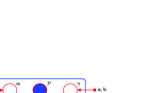
Figure 1: Graphical representation of the RSM model.

We point out that the choice of separating the role of the known subgraphs and the latent clusters was motivated by historical assumptions on the creation of relationships between individuals in Gaul during the $6$th century. These assumptions were at the core of the study of the ecclesiastical network we consider in this paper. An alternative approach would consist in allowing the presence of an edge and its type to depend on both the subgraphs and latent clusters. However, this would dramatically increase the number of model parameters to be estimated. Indeed, for a network with $S=6$, $K=6$, and $C=4$, it would require $K^{2}S^{2}(C+1)+SK=6516$ parameters while RSM only involves $S^{2}+K^{2}C+SK=216$ parameters.

2.2 Bayesian framework

We consider a Bayesian framework and introduce conjugate prior distributions. Thus, since $\mathbf{Z}_{i}$ is sampled from a multinomial distribution, we rely on a Dirichlet prior to model the parameters $\bolds{\alpha}_{s}$:

$$p(\bolds{\alpha}_{s})=\operatorname{Dir}\bigl{(}\bolds{\alpha}_{s};\chi_{s1}^{0},\ldots,\chi_{sK}^{0}\bigr{)}\qquad\forall s\in\{1,\ldots,S\}.$$

A similar distribution is used as a prior distribution for the parameters $\bolds{\Pi}_{kl}$:

$$p(\bolds{\Pi}_{kl})=\operatorname{Dir}\bigl{(}\bolds{\Pi}_{kl};\Xi_{kl1}^{0},\ldots,\Xi_{klC}^{0}\bigr{)}\qquad\forall(k,l)\in\{1,\ldots,K\}^{2}.$$

If no prior information is available, a common choice in the literature consists in fixing the hyperparameters of the Dirichlet to $1/2$, that is, $\chi_{sk}^{0}=1/2,\forall(s,k)$ and $\Xi_{klc}=1/2,\forall(k,l,c)$. Such a distribution corresponds to a noninformative Jeffreys prior distribution which is known to be proper [Jeffreys (1946)]. A uniform distribution can also be obtained by setting the hyperparameters to $1$.

Finally, since the presence or absence of an edge between a pair of vertices is drawn from a Bernoulli distribution, we rely on a beta prior for the parameters $\gamma_{rs}$:

$$p(\gamma_{rs})=\operatorname{Beta}\bigl{(}\gamma_{rs};a_{rs}^{0},b_{rs}^{0}\bigr{)}\qquad\forall(r,s)\in\{1,\ldots,S\}^{2}.$$

Again, if no prior information is available, both hyperparameters $a_{rs}^{0}$ and $b_{rs}^{0}$ can be set to $1/2$ or $1$ to obtain noninformative prior distributions, respectively, a Jeffreys or a uniform distribution. Figure 1 presents the graphical model associated with the RSM model.

2.3 Inference with the variational Bayes EM algorithm

Given the observed matrices $\mathbf{X}$ and $\mathbf{A}$, we aim at estimating the posterior distribution$p(\mathbf{Z},\bolds{\alpha},\bolds{\gamma},\bolds{\Pi}|\mathbf{X},\mathbf{A})$, which in turn will allow us to compute a maximum a posteriori estimate of the clustering structure $\mathbf{Z}$ as well as the parameters $(\bolds{\alpha},\bolds{\gamma},\bolds{\Pi})$. Because this distribution is not tractable, approximate inference procedures are required. The Markov chain Monte Carlo (MCMC) sampling scheme is a widely used approach which consists in sampling from tractable conditional distributions. After a burn-in period, samples are assumed to be drawn from the true posterior distribution. One of the main advantages of the MCMC algorithm is that it can characterize the uncertainty in model parameters. Moreover, the convergence of the Markov chain and therefore the quality of the approximation can be tested.

Unfortunately, the MCMC algorithm has a poor scaling with sample sizes. This motivated the work of Daudin, Picard and Robin (2008) who proposed a variational approach for the SBM model which can deal with large networks contrary to the MCMC method of Nowicki and Snijders (2001). In general, the main drawback of variational techniques is that, although they can produce a good estimate of the model parameters or find the mode of the posterior distribution, they usually cannot uncover the uncertainty in the model parameters and tend to underestimate posterior variances. Furthermore, the quality of the variational approximation cannot be tested in most cases since the KL divergence between the true and approximate posterior distribution is not tractable.

However, recent results [Celisse, Daudin and Pierre (2012), Mariadassou and Matias (2014)] gave some new insights on the form of the true posterior distribution in the case of the SBM model and showed that the corresponding variational estimates were consistent. In light of these recent results and because we aim at proposing an inference procedure capable of handling large networks, we rely in the following on a variational Bayes EM (VBEM) algorithm.

Thus, given a distribution $q(\mathbf{Z},\bolds{\alpha},\bolds{\gamma},\bolds{\Pi})$, the marginal log-likelihood can be computed in two terms,

$$\log p(\mathbf{X},\mathbf{A})=\mathcal{L}(q)+\mathrm{KL}\bigl{(}q(\cdot)\|p(\cdot|\mathbf{X},\mathbf{A})\bigr{)},$$

where $\mathcal{L}$ is defined as follows:

$$\mathcal{L}(q)=\sum_{\mathbf{Z}}{\int_{\bolds{\alpha},\bolds{\gamma},\bolds{\Pi}}{q(\mathbf{Z},\bolds{\alpha},\bolds{\gamma},\bolds{\Pi})\log\biggl{(}\frac{p(\mathbf{X},\mathbf{A},\mathbf{Z},\bolds{\alpha},\bolds{\gamma},\bolds{\Pi})}{q(\mathbf{Z},\bolds{\alpha},\bolds{\gamma},\bolds{\Pi})}\biggr{)}\,d\bolds{\alpha}\,d\bolds{\gamma}\,d\bolds{\Pi}}}$$

and the KL divergence is given by

$$\mathrm{KL}\bigl{(}q(\cdot)\|p(\cdot|\mathbf{X})\bigr{)}$$

$$\qquad=-\sum_{\mathbf{Z}}{\int_{\bolds{\alpha},\bolds{\gamma},\bolds{\Pi}}{q(\mathbf{Z},\bolds{\alpha},\bolds{\gamma},\bolds{\Pi})\log\biggl{(}\frac{p(\mathbf{Z},\bolds{\alpha},\bolds{\gamma},\bolds{\Pi}|\mathbf{X},\mathbf{A})}{q(\mathbf{Z},\bolds{\alpha},\bolds{\gamma},\bolds{\Pi})}\biggr{)}\,d\bolds{\alpha}\,d\bolds{\gamma}\,d\bolds{\Pi}}}.$$

Finding the best approximation of the posterior distribution $p(\mathbf{Z},\bolds{\alpha},\bolds{\gamma},\bolds{\Pi}|\mathbf{X},\mathbf{A})$ in the sense of the KL divergence becomes equivalent to finding $q(\cdot)$ that maximizes the lower bound $\mathcal{L}(q)$ of the integrated log-likelihood. To obtain a tractable algorithm, we assume that $q(\cdot)$ can be fully factorized, that is,

$$q(\mathbf{Z},\bolds{\alpha},\bolds{\gamma},\bolds{\Pi})=\Biggl{(}\prod_{i=1}^{N}{q(\mathbf{Z}_{i})}\Biggr{)}\Biggl{(}\prod_{s=1}^{S}{q(\bolds\alpha_{s})\prod_{t=1}^{S}{q(\gamma_{s,t})}}\Biggr{)}\prod_{k,l}^{K}{q(\bolds\Pi_{k,l})}.$$

The functional optimization of the lower bound with respect to $q(\cdot)$ is performed using a VBEM algorithm (see Algorithm 1). All the optimization equations are given in the Appendix. We emphasize that the functional form of the prior distributions is preserved through the optimization. In particular, $q(\mathbf{Z})$ is given by

$$q(\mathbf{Z})=\prod_{i=1}^{N}q(\mathbf{Z}_{i})=\prod_{i=1}^{N}\mathcal{M}(\mathbf{Z}_{i};1,\bolds{\tau}_{i}),$$

where $\tau_{ik}$ is a variational parameter denoting the probability of node $i$ to belong to cluster $k$. The approximate posterior distributions over the other model parameters $(\bolds{\alpha},\bolds{\gamma},\bolds{\Pi})$ depend on parameters that we denote $\bolds{\theta}=\{\bolds{\chi},(\mathbf{a},\mathbf{b}),\bolds{\Xi}\}$, respectively.

Algorithm 1 VBEM algorithm for the RSM model (see text for details)

  Initialize matrix $\bolds{\tau}=\mathbf{Z}$ with k-means

  Initialize hyperparameters $\bolds{\theta}^{0}=\{\bolds{\chi}^{0},(\mathbf{a}^{0},\mathbf{b}^{0}),\bolds{\Xi}^{0}\}$

  Compute $\mathcal{L}(q)$

  while $|\bolds{\theta}^{\mathrm{new}}-\bolds{\theta}^{\mathrm{old}}|\geq\varepsilon$ do

     E step: update $\bolds{\tau}$

     M step: update $\bolds{\theta}^{\mathrm{new}}=\{\bolds{\chi},(\mathbf{a},\mathbf{b}),\bolds{\Xi}\}$

     Compute $\mathcal{L}$

  end while

2.4 Initialization

The VBEM algorithm, though useful in approximating posterior distributions of graphical models, is only guaranteed to converge to a local optimum [Bilmes (1998)]. Strategies to tackle this issue include simulated annealing and the use of multiple initializations [Biernacki, Celeux and Govaert (2003)]. In this work, we choose the latter option. In order to have a better chance of reaching a global optimum, VBEM is run for several initializations of a k-means like algorithm with the following distance $d(i,j)$ between the vertices $i$ and $j$:

$$d(i,j)=\sum_{h=1}^{N}\delta(X_{ih}\neq X_{jh})A_{ih}A_{jh}+\sum_{h=1}^{N}\delta(X_{hi}\neq X_{hj})A_{hi}A_{hj}.$$ (1)

The first term looks at all possible edges from $i$ and $j$ toward a third vertex $h$. If both $i$ and $j$ are connected to $h$, that is, $A_{ih}A_{jh}=1$, the edge types $X_{ih}$ and $X_{jh}$ are compared. By symmetry, the second term looks at all possible edges from a vertex $h$ to both $i$ as well as $j$, and compare their types. Thus, the distance computes the number of discordances in the way both $i$ and $j$ connect to other vertices or vertices connect to them. The algorithm starts by sampling the cluster centers among all the vertices of the network. It then iterates a two-step procedure until convergence of the cluster centers. In the first step, the vertices are classified into the cluster with the closest center. Each cluster center is then associated to a vertex minimizing its distance with all the vertices of the corresponding cluster.

2.5 Choice of $K$

So far, the number $K$ of latent clusters has been assumed to be known. Given $K$, we showed in Section 2.3 how an approximation of the posterior distribution over the latent structure and model parameters could be obtained. We now address the problem of estimating the number of clusters directly from the data. Given a set of values of $K$, we aim at selecting $K^{*}$ for which the marginal log-likelihood $\log p(\mathbf{X}|K)$ is maximized. However, because this integrated log-likelihood involves a marginalization over all the model parameters and latent variables, it is not tractable. Therefore, we propose to replace the marginal log-likelihood with its variational approximation, as in Bishop (2006), Latouche, Birmelé and Ambroise (2009, 2012). Thus, for each value of $K$ considered, the VBEM algorithm is applied. We recall that the maximization of the lower bound induces a minimization of the KL divergence. After convergence of the algorithm, the lower bound is used as an approximation of $\log p(\mathbf{X}|K)$ and $K$ is chosen such that the lower bound is maximized. We prove in the Appendix that, if computed right after the M step of the variational Bayes EM, the lower bound has the following expression:

$$\mathcal{L}(q) = \sum_{r,s}^{S}\log\biggl{(}\frac{B(a_{rs},b_{rs})}{B(a_{rs}^{0},b_{rs}^{0})}\biggr{)}+\sum_{s=1}^{S}\log\biggl{(}\frac{C(\bolds\chi_{s})}{C(\bolds\chi_{s}^{0})}\biggr{)}$$

$${}+\sum_{k,l}^{K}\log\biggl{(}\frac{C(\bolds\Xi_{kl})}{C(\bolds\Xi_{kl}^{0})}\biggr{)}-\sum_{i=1}^{N}\sum_{k=1}^{K}\tau_{ik}\log(\tau_{ik}),$$

where $C(x)=\frac{\prod_{d=1}^{D}\Gamma(x_{d})}{\Gamma(\sum_{d=1}^{D}x_{d})}$ if $x\in\mathbb{R}^{D}$, $B(a,b)=\frac{\Gamma(a)\Gamma(b)}{\Gamma(a+b)},\forall(a,b)\in\mathbb{R}^{2}$, and $\Gamma(\cdot)$ is the gamma function. See the Appendix for the definition of $a_{rs}$, $b_{rs}$, $\bolds{\chi_{s}}$, $\bolds{\Xi_{kl}}$ and $\tau_{ik}$.

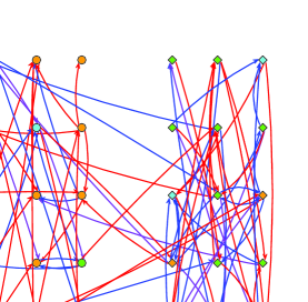
Figure 2: Example of a RSM network for $S=2$ subgraphs (indicated by the node forms), $C=3$ types of edges (indicated by the edge colors) and $K=3$ clusters to identify (indicated by the node colors).

3 Numerical experiments and comparisons

In this section we first run experiments aimed at proving the validity of our model, focusing on the ability of its inference procedure to find the right clustering. We then compare its performance to that of other stochastic models for graph clustering.

3.1 Experimental setup

In order to evaluate the performance of our approach, we applied it on data generated according to the RSM model. To simplify the parameterization and facilitate the reproducibility of the experiments, we constrained the parameters $\bolds\Pi$ and $\bolds{\gamma}$ to have the following forms:

$$\bolds{\Pi}=\left[\matrix{\mathbf{u}&\mathbf{v}&\cdots&\mathbf{v}\cr\mathbf{v}&\mathbf{u}&\ddots&\vdots\cr\vdots&\ddots&\ddots&\mathbf{v}\cr\mathbf{v}&\cdots&\mathbf{v}&\mathbf{u}}\right],\qquad\bolds{\gamma}=\left[\matrix{\lambda&\varepsilon&\cdots&\varepsilon\cr\varepsilon&\lambda&\ddots&\vdots\cr\vdots&\ddots&\ddots&\varepsilon\cr\varepsilon&\cdots&\varepsilon&\lambda}\right],$$

where $\lambda$, $\varepsilon\in[0,1]$ and $\mathbf{u},\mathbf{v}\in[0,1]^{K}$. With such a parameterization, the probability $\lambda$ of an edge within a subgraph is assumed to be common between subgraphs and the probability $\varepsilon$ of a connection between different subgraphs is also assumed to be the same for all couples of subgraphs. Similarly, the vector $\mathbf{u}$ controls the probability of each edge type between nodes of a same cluster, whereas $\mathbf{v}$ defines the edge type probabilities between nodes of different clusters. We recall that the prior probabilities of each group within each subgraph are given by the parameter $\bolds{\alpha}=(\bolds{\alpha}_{1},\ldots,\bolds{\alpha}_{S})$.

Figure 2 presents an example of a network generated this way with parameters $S=2$, $C=3$, $K=3$, $\bolds{\alpha}=\bigl{[}{{\matrix{0.1\ \ 0.3\ \ 0.6\cr 0.6\ \ 0.3\ \ 0.1}}}\bigr{]}$, $\lambda=0.6$, $\varepsilon=0.06$, $\mathbf{u}=(0.8,0.1,0.1)$ and $\mathbf{v}=(0.1,0.3,0.6)$. This RSM network is made of 30 nodes with $S=2$ subgraphs (indicated by the node forms), $C=3$ types of edges (indicated by the edge colors) and $K=3$ clusters that have to be identified in practice (indicated by the node colors).

In order to illustrate, on various situations, that RSM is a relevant model and that its corresponding inference procedure provides an accurate estimation of the true clustering structure, we rely in the following paragraphs on three types of graphs, described in Table 2. The three scenarios considered correspond to different situations ranging from an almost classical setup to a more specific one. The first scenario considers networks with no subgraphs ($S=1$) and with a preponderant proportion of edges of type 1 ($u_{1}=0.8$) and 3 ($u_{3}=0.8$). The second scenario still considers networks with no subgraphs ($S=1$) but with balanced proportions of edge types. Finally, the third scenario considers networks with several subgraphs ($S=3$) and balanced proportions for edge types. Therefore, the latter case should be the more complex situation to fit.

=253pt Parameters Scenario 1 Scenario 2 Scenario 3 $N$ 100 100 100 $S$ 001 001 003 $C$ 003 003 003 $K$ 003 003 003 $\bolds{\alpha}$ (0.3, 0.3, 0.4) (0.3, 0.3, 0.4) $\left[\matrix{0&0.5&0.5\cr 0.5&0&0.5\cr 0.5&0.5&0}\right]$ $\mathbf{u}$ (0.8, 0.1, 0.1) (0.5, 0.45, 0.05) (0.5, 0.45, 0.05) $\mathbf{v}$ (0.1, 0.1, 0.8) (0.1, 0.45, 0.45) (0.1, 0.45, 0.45) $\lambda$ 0.20 0.20 0.2 $\varepsilon$ 0.06 0.06 0.1

Table 2: Parameter values for the three types of graphs used in the experiments

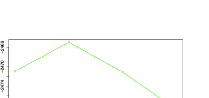
Figure 3: Criterion values $\mathcal{L}(q)$ vs. number $K$ of groups for a graph simulated according to scenario 1.

The VBEM algorithm with multiple initializations, presented in Section 2, is used in the following experiments. For a given value of $K$, the result with the best value for $\mathcal{L}(q)$ is chosen among the multiple initializations. Then, a clustering partition is deduced from the posterior probabilities $\tau_{ik}$ using the maximum a posteriori (MAP) rule, that is, a node is assigned to the group with the highest posterior probability.

Since our approach aims to search the unobserved clustering partition of the nodes, we chose here to evaluate the results of our VBEM algorithm by comparing the resulting partition with the actual one (the simulated partition). In the clustering community, the adjusted Rand index (ARI) [Rand (1971)] serves as a widely accepted criterion for the difficult task of clustering evaluation. The ARI looks at all pairs of nodes and checks whether they are classified in the same group or not in both partitions. As a result, an ARI value close to 1 means that the partitions are similar and, in our case, that the VBEM algorithm succeeds to recover the simulated partition.

3.2 Choice of $K$ and inference results

In this first simulation study we aim at evaluating the ability of the lower bound $\mathcal{L}(q)$ to serve as a criterion for selecting the appropriate number $K$ of clusters. To this end, the VBEM algorithm for the RSM model was first run on a graph simulated according to scenario 1 for several values of $K$. The highest criterion values among the different initializations obtained for each value of $K$ are presented in Figure 3. The figure indicates that $K=3$ seems to be the appropriate number of groups for the studied network, which is the actual number of group.

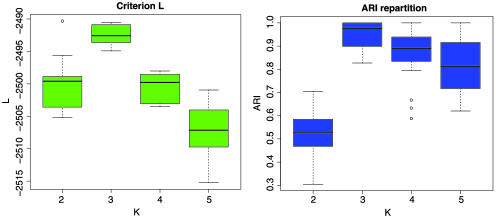
Figure 4: Repartition of the criterion (left panel) and ARI (right panel) over 50 networks generated with the parameters of the first scenario.

We then replicated this experiment over 50 networks, still simulated according to scenario 1, for both verifying the consistency of $\mathcal{L}(q)$ and studying the clustering ability of our approach. Figure 4 shows the repartition of the criterion values (left panel) as well as the associated ARI values (righ panel). These results confirm that the lower bound $\mathcal{L}(q)$ is a valid criterion for selecting the number of groups. One can also observe that the partition resulting from our VBEM algorithm has, for the selected number of groups, a good adequation with the actual partition of the data.

3.3 Comparison with the stochastic block model

Our second set of experiments compares the performance of RSM to that of other models on data drawn according to its generative process. We were interested in the comparison with the following models:

• binary SBM (presence): We fit a binary SBM using the R package mixer [Ambroise et al. (2010)] on a collapsed version of the data to conform this specific model. The collapsed data were obtained by considering only the presence of the edges and not the type of the edges, that is, $\tilde{X}_{ij}=0$ if $X_{ij}=0$ and $\tilde{X}_{ij}=1$ otherwise.

• binary SBM (type 1, 2 or 3): We fit a binary SBM, still using the mixer package, on the networks defined by taking only the edges of one type. For instance, the collapsed network for type $c=1,2,3$ was obtained by considering only the presence of type $c$ edges, that is, $\tilde{X}_{ij}=1$ if $X_{ij}=c$ and $\tilde{X}_{ij}=0$ otherwise.

• typed SBM: We consider here a SBM with discrete edges. Although SBM was originally proposed in Nowicki and Snijders (2001) with discrete edges, existing softwares only propose to fit a SBM on binary networks. We therefore had to implement a version of the SBM which supports typed edges. Note that, in this case, the types of edges are in $\{0,\ldots,C\}$, where 0 corresponds to the absence of a relation.

• RSM: We run the VBEM algorithm, that we proposed in Section 2 for the inference of the RSM model, with the available subgraph partition and with 5 random initializations for each run.

Table 3: Average ARI values and standard deviations for binary SBM, typed SBM and RSM according to the three simulation scenarios. The results are averaged on 25 simulated graphs for each scenario

Method	Scenario 1	Scenario 2	Scenario 3
Binary SBM (presence)	0.001${}\pm{}$0.012	$-$0.001${}\pm{}$0.013	$-$0.239${}\pm{}$0.061
Binary SBM (type 1)	0.976${}\pm{}$0.071	$-$0.494${}\pm{}$0.233	$-$0.372${}\pm{}$0.262
Binary SBM (type 2)	0.001${}\pm{}$0.006	$-$0.003${}\pm{}$0.006	$-$0.179${}\pm{}$0.097
Binary SBM (type 3)	0.959${}\pm{}$0.121	$-$0.519${}\pm{}$0.219	$-$0.367${}\pm{}$0.244
Typed SBM	0.694${}\pm{}$0.232	$-$0.472${}\pm{}$0.339	$-$0.360${}\pm{}$0.162
RSM	1.000${}\bolds{\pm}{}$0.000	$-$0.981${}\bolds{\pm}{}$0.056	$-$0.939${}\bolds{\pm}{}$0.097

Table 3 presents the average ARI values and standard deviations on 50 simulated graphs for each scenario and with binary SBM, typed SBM and RSM. We point out that the inference is done with the actual number of clusters and this for each method. One can observe that, for the first scenario, the binary SBM based on the link presences and the type 2 SBM always fails, whereas type 1, type 3 and typed SBM work pretty well. Those behaviors can be explained by the nature of scenario 1, which is a rather easy situation with no subgraphs and a predominant presence of type 1 and type 2 links. However, we can remark that it seems easier in this case to fit a binary SBM on type 1 or type 2 edges than to fit a typed SBM. This is due to the high discriminative power of type 1 and type 2 edges in this specific scenario. Let us also remark that RSM works perfectly here even though the network does not contain any subgraphs.

Regarding scenario 2, which considers a situation where there is still no subgraphs but with more balanced proportions of the different edge types, one can first notice that binary SBM and type 2 SBM fail once again. The type 1 and type 3 SBM have now a behavior closer to the one of typed SBM, whereas RSM gives very accurate results once again. Finally, scenario 3 considers a RSM-type network, that is, with several subgraphs, and all SBM-based algorithms are significantly outperformed by RSM, which succeeds in exploiting both the information carried by different edge types and by the different subgraphs. To summarize, the RSM model and its associated VBEM algorithm turn out to be effective on situations ranging from classical setups without subgraphs to complex scenarios with subgraphs and typed edges.

4 Ecclesiastical network

This section now focuses on applying the RSM model to the ecclesiastical network, that we briefly described in the Introduction and that initially motivated this work, and on analyzing its results from the historical point of view.

Please note that the ecclesiastical network along with a file giving the kingdoms of all vertices in the network and an R code implementing the variational inference approach for the RSM model are provided as supplementary materials in Jernite et al. (2013).

4.1 Description of the data

The relational data considered in this section were mainly built from written acts of ecclesiastical councils that took place in Merovingian Gaul during the 6th century. A council is an ecclesiastical meeting, usually called by a bishop, where issues regarding the Church or the faith are addressed. However, since 511, kings could also call for a council to discuss some political, judiciary or legal issues, and that laics (kings, dukes or counts, e.g.) would attend. During the 6th century, 46 councils took place in Gaul. Although there were mostly local or regional councils, attended by individuals from a specific ecclesiastical province, there were some national councils convened under the authority of a king.

The composition of these councils is known thanks to the acts written at the end of the meeting, and which were signed by all attending members. In addition to the council acts, we used narrative texts (among which is the famous Ten History Books by Gregory of Tours), hagiographies or letters which also describe these councils. The network, that took over 18 months to build from these historical sources, contains $N=1331$ individuals who held one or several offices in Gaul between the years 480 and 614, and who we know to have been related or to have met during their lifetime.

The council acts and the other historical sources allowed also to qualify the type of the relationship between the individuals involved in the network. However, the scarcity of the sources only allowed for an approximate characterization of these relationships. As a consequence, $C=4$ relation types were qualified and the relationships can be either positive, negative, variable or neutral (when the type was unknown). For instance, a positive relationship may describe an agreement between two clergymen on a question of faith, whereas a negative one may be a disagreement on such a question. Variable relationships usually correspond to relationships which change over time.

Using the different sources, it was also possible to obtain additional information on the individuals. In particular, the geographical positions of the offices hold by the clergymen or the laics allowed us to split the network into $S=6$ subgraphs. Those 6 subgraphs correspond to the geographical partition of the Gaul at this period (the kingdoms of Neustria, Austrasia and Burgondy, and the provinces of Aquitaine and Provence), completed with an additional subgraph for individuals for whom the information was not available. We also recorded the social positions of the individuals in order to be able to interpret afterward the clusters found by our method. These social positions can be, for instance, ecclesiastical positions (bishops, deacon, archdeacon, abbot, priest$,\ldots$) or titles of nobility (king, queen, duke, earl$,\ldots$).

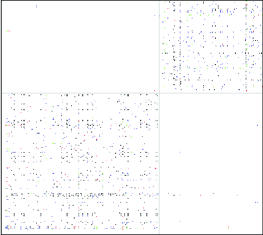
Figure 5: Adjacency matrix for the kingdom of Neustria (left block) and the province of Provence (right block). The dot colors indicate the type or relationships: red${}={}$“negative,” green${}={}$“variable,” black${}={}$“neutral” and blue${}={}$“positive.” Zoom on the paper electronic version for details.

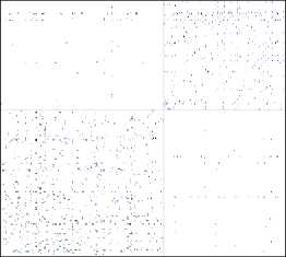
Figure 6: Adjacency matrix for the kingdoms of Austrasia (left block) and Burgundy (right block). The dot colors indicate the type or relationships: red${}={}$“negative,” green${}={}$“variable,” black${}={}$“neutral” and blue${}={}$“positive.” Zoom on the paper electronic version for details.

To summarize, the network is made of $N=1331$ individuals split into $S=6$ subgraphs and whose relationships can be of $C=4$ difference types. Figures 5 and 6 show some parts of the whole adjacency matrix associated to the network where the dot colors indicate the type or relationships. The whole adjacency matrix is provided in a zoomable pdf file as supplementary material [Jernite et al. (2013)]. We expect the statistical analysis with RSM of this network to help us understand how the behavior of an individual can be modeled through their belonging to a group. The use of a probabilistic approach, instead of a deterministic one, makes particular sense here since at least a part of the historical sources are subject to caution due to their nature and age. In History, this kind of approach is more common to modernists or contemporarists than to medievists who rarely have access to this kind of data. Let us finally notice that a “source effect” is expected due to the possible overrepresentation in our sources of some places (Neustria by Gregory of Tours or Austrasia by Fredegar) or some individuals (in letters or hagiographies).

4.2 Results

The VBEM algorithm that we proposed to infer the RSM model was run on the network defined by these relations, where the subgraphs are the provinces in which the individuals lived (Aquitaine, Austrasia, Burgondy, Neustria, Provence or Unknown). The use of the lower bound $\mathcal{L}(q)$ allowed us to find 6 clusters.

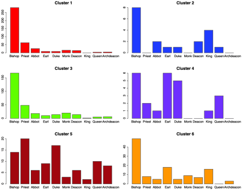
Figure 7: Repartition of the different social positions in the found clusters (restricted to the 10 most frequent positions).

To give some insight into the nature of the found clusters, Figure 7 presents the repartition of the different social positions in the clusters. In view of these results, some historical comments can be done. First, clusters 1 and 3 appear to be made of the people who would attend local assemblies, provincial or diocesan councils. The council of Arles, which took place in 554, would have had the same kind of composition as cluster 3, while that of Auxerre, in 585, could well represent cluster 1. Second, clusters 4 and 5 are more characteristic of aristocratic assemblies, such as the council of Orange in 529. Third, clusters 2 and 6 have the same compositions as councils concerned with more political issues (those usually convened by a king). Such a council took place in Orleans in 511. Let us, however, notice that cluster 2 is composed of very few individuals, which might hurt the relevance of its interpretation. Also, we might be able to further our understanding of the composition of these clusters by taking into account the similarity of certain social positions (such as “duke” and “earl”).

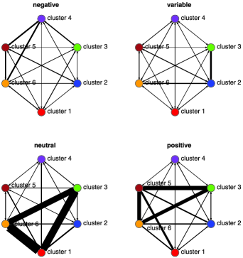
Figure 8: Relations between the 6 found clusters (parameter $\bolds{\Pi}$) for each relation type: negative, variable, neutral and positive. For visualization purposes, the relation weights have been normalized according to relation types.

The relations between the different clusters, described by the parameter $\bolds{\Pi}$ and shown in Figure 8, inform us further. Although the limitations expressed above about the roughness of the relation types still apply, they nevertheless provide us with interesting elements to confirm the coherence of the proposed model. First, it is natural that we should find “neutral” relations at the local level, between clusters 1, 3 and 6. Indeed, local assemblies were the less documented ones in our sources. On the other hand, the links between high level individuals are better known, because councils used to settle conflicts between aristocrats, which explains the presence of “negative” and “variable” relations. Finally, the positive relations between cluster 3, 5 and 6 could represent the personal friendships documented by a collection of letters between bishops.

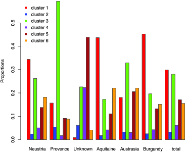
Figure 9: Repartition of the 6 found clusters in the different Provinces (parameter $\bolds{\alpha}$).

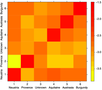
Figure 10: Estimated values for the parameter $\bolds{\gamma}$ (in log scale).

After having described the political background represented by each of the clusters, we can compare the organization of the different regions. Figure 9 presents the cluster repartition (parameter $\bolds{\alpha}$) in the different provinces. One can observe that the clergy and noblemen of the different regions were concerned with very different issues: Provence and Burgundy were more concerned with local questions (clusters 1 and 3), and less with political ones (clusters 2 and 6). The clusters concerned both with local (clusters 1 and 3) and high level (cluster 6) questions are represented in Aquitaine. Conversely, all levels of power are represented in Neustria. This could be the result of a “source effect,” as mentioned above. Let us also notice that the council structures seem similar in Austrasia and Aquitaine: sovereigns (kings and queens) are involved in the Church and frequently convene councils in order to discuss political questions.

Some of these observations are confirmed by the estimate of parameter $\bolds{\gamma}$, which is given in a log scale by Figure 10. First, it shows a greater frequency of relations between Aquitaine and Neustria, which comes both from a geographical and political proximity (Aquitaine is absorbed into Clovis’ kingdom in 507, then divided and absorbed by Neustria in 511). One can also see there another example of “source” effect, as our main source, Gregory of Tours, was bishop in Neustria and raised in Aquitaine (next to his uncle, the bishop of Clermont), which gave him a good knowledge of both provinces. More enlightening is the relative disconnection of Burgondy and Provence, especially in regard to the provinces of Austrasia and Neustria, both heavily connected.

4.3 Conclusion from the historical point of view

A first analysis of the results of the RSM model confirms two well-known general facts. Indeed, our results confirm the preponderance of local assemblies in 6th century Gaul and the “source effect.” Nevertheless, further analysis of the found clusters and their relations yields a better understanding of the period. In particular, the composition of the found clusters reflect different archetypes of councils and different levels of political concerns. Our results have also highlighted that the types of concerns of each province are closely related to the frequency of their communications with others.

Two limitations to these results remain, however. First, we are limited by the scarcity of the historical documentation. It would be interesting to see whether the use of more precise types of relations (ecclesiastical or secular, through which media$,\ldots$) could improve the results. Second, it would also be interesting for the model to take into account temporal evolutions of the relations and clusters. Indeed, one aspect of the data which is currently not addressed by the results of RSM is its temporality. Nevertheless, this lack seems to have a limited impact here since all clusters exhibit the same distribution of individuals over time, reflecting the higher concentration of information in years 550 to 600 (when numerous conflicts were settled by councils: Paris 577, Chalon 579, Berny 580, Lyon 581$,\ldots$). The repartition of the different kinds of powers then seems to change little over time on this short period.

5 Conclusion and further work

In this work we proposed a new stochastic graph model, the random subgraph model, to deal with networks where a vertex behavior is influenced by an observed partition variable. We derived a variational Bayes EM algorithm to infer the model parameters from data and applied it to an ecclesiastical network from Merovingian Gaul. The results of the fitted RSM enlightened us on the different levels of power present at this time in Gaul, and on the different power structures of different regions. Let us highlight that the RSM model allows in addition the comparison of subgraphs through the model parameters, in particular, the cluster proportions. We also would like to mention that networks with typed edges and subgraphs can be encountered in many application fields (such as biology, economics, archeology$,\ldots$) and the RSM model should be useful in these contexts as well.

One aspect, however, that RSM does not currently address is the temporality of the data. Since this aspect can be found in many of the data sets we wish to apply the RSM model to, we believe that a natural continuation of this work would be a dynamic extension of the RSM model. Moreover, we plan to introduce a Chinese restaurant process on the latent cluster structure in order to automatically estimate the number of clusters while clustering the vertices. Finally, we would like to consider the problem of visualizing such networks with typed edges and known subgraphs.

Appendix: Variational Bayes

In this final section we detail the computations that lead to the update rules given in Section 2, and provide an explicit expression of the criterion $\mathcal{L}(q)$.

Proposition .1

The complete data log-likelihood the RSM model is given by

$$\log p(\mathbf{X},\mathbf{A},\mathbf{Z},\bolds{\alpha},\bolds{\gamma},\bolds{\Pi})$$

$$\qquad=\sum_{i\neq j}^{N}\sum_{c=1}^{C}\sum_{k,l}^{K}\bigl{\{}\delta(X_{ij}=c)Z_{ik}Z_{jl}\log(\Pi_{klc})\bigr{\}}$$

$$\quad\qquad{}+\sum_{i=1}^{N}\sum_{k=1}^{K}Z_{ik}\log(\alpha_{r_{i},k})$$

$$\quad\qquad{}+\sum_{i\neq j}^{N}\bigl{\{}A_{ij}\log(\gamma_{r_{i},r_{j}})+(1-A_{ij})\log(1-\gamma_{r_{i},r_{j}})\bigr{\}}$$

$$\quad\qquad{}+\sum_{s=1}^{S}\log p(\bolds{\alpha}_{s})+\sum_{r,s}^{S}\log p(\gamma_{rs})+\sum_{k,l}^{K}\log p(\bolds{\Pi}_{kl}).$$

$$\log p(\mathbf{X},\mathbf{A},\mathbf{Z},\bolds{\alpha},\bolds{\gamma},\bolds{\Pi})$$

$$\qquad=\log p(\mathbf{X}|\mathbf{A},\mathbf{Z},\bolds{\Pi})+\log p(\mathbf{A}|\bolds{\gamma})+\log p(\mathbf{Z}|\bolds{\alpha})+\log p(\bolds{\alpha})+\log p(\bolds{\gamma})$$

$$\quad\qquad{}+\log p(\bolds{\Pi})$$

$$\qquad=\sum_{i\neq j}^{N}\sum_{c=1}^{C}\sum_{k,l}^{K}\bigl{\{}\delta(X_{ij}=c)Z_{ik}Z_{jl}\log(\Pi_{klc})\bigr{\}}$$

$$\quad\qquad{}+\sum_{i=1}^{N}\sum_{k=1}^{K}Z_{ik}\log(\alpha_{r_{i},k})$$

$$\quad\qquad{}+\sum_{i\neq j}^{N}\bigl{\{}A_{ij}\log(\gamma_{r_{i},r_{j}})+(1-A_{ij})\log(1-\gamma_{r_{i},r_{j}})\bigr{\}}$$

$$\quad\qquad{}+\sum_{s=1}^{S}\log p(\bolds{\alpha}_{s})+\sum_{r,s}^{S}\log p(\gamma_{rs})+\sum_{k,l}^{K}\log p(\bolds{\Pi}_{kl}).$$

Proposition .2

The VBEM update step for the distribution $q(\gamma_{rs})$ is given by

$$q(\gamma_{rs})=\operatorname{Beta}(\gamma_{rs};a_{rs},b_{rs})\qquad\forall(r,s)\in\{1,\ldots,S\}^{2},$$

where

$$a_{rs}=a_{rs}^{0}+\sum_{r_{i}=r,r_{j}=s}(A_{ij})$$

and

$$b_{rs}=b_{rs}^{0}+\sum_{r_{i}=r,r_{j}=s}(1-A_{ij}).$$

$$\log q(\gamma_{rs})$$

$$\qquad=\mathbb{E}_{\mathbf{Z},\bolds{\alpha},\bolds{\gamma}^{\setminus rs},\bolds{\Pi}}\bigl{[}\log p(\mathbf{X},\mathbf{A},\mathbf{Z},\bolds{\alpha},\bolds{\gamma},\bolds{\Pi})\bigr{]}+\kappa$$

$$\qquad=\sum_{r_{i}=r,r_{j}=s}\bigl{\{}A_{ij}\log(\gamma_{rs})+(1-A_{ij})\log(1-\gamma_{rs})\bigr{\}},$$

$$\log p(\gamma_{rs})+\kappa$$

$$\qquad=\sum_{r_{i}=r,r_{j}=s}\bigl{\{}A_{ij}\log(\gamma_{rs})+(1-A_{ij})\log(1-\gamma_{rs})\bigr{\}},$$

$$\bigl{(}a_{rs}^{0}-1\bigr{)}\log(\gamma_{rs})+\bigl{(}b_{rs}^{0}-1\bigr{)}\log(1-\gamma_{rs})+\kappa$$

$$\qquad=\biggl{(}a_{rs}^{0}-1+\sum_{r_{i}=r,r_{j}=s}A_{ij}\biggr{)}\log(\gamma_{rs})$$

$$\quad\qquad{}+\biggl{(}b_{rs}^{0}-1+\sum_{r_{i}=r,r_{j}=s}(1-A_{ij})\biggr{)}\log(1-\gamma_{rs})+\kappa,$$

where $\kappa$ is a constant term. Hence, the functional form of the variational approximation $q(\gamma_{rs})$ corresponds to a Beta distribution with updated hyperparameters:

$$a_{rs}=a_{rs}^{0}+\sum_{r_{i}=r,r_{j}=s}(A_{ij})$$

and

$$b_{rs}=b_{rs}^{0}+\sum_{r_{i}=r,r_{j}=s}(1-A_{ij}).$$

Proposition .3

The VBEM update step for the distribution $q(\mathbf{Z}_{i})$ is given by

$$q(\mathbf{Z}_{i})=\mathcal{M}(\mathbf{Z}_{i};1,\bolds{\tau}_{i})\qquad\forall i,$$

where

$$\tau_{ik} \propto \exp\Biggl{(}\psi(\chi_{r_{i},k})-\psi\Biggl{(}\sum_{l=1}^{K}\chi_{r_{i},l}\Biggr{)}\Biggr{)}$$

$${}+\exp\Biggl{\{}\sum_{j\neq i}^{N}\sum_{c=1}^{C}\sum_{l=1}^{K}\delta(X_{ij}=c)\tau_{jl}\Biggl{(}\psi(\Xi_{klc})-\psi\Biggl{(}\sum_{u=1}^{C}\Xi_{klu}\Biggr{)}\Biggr{)}\Biggr{\}}$$

$${}+\exp\Biggl{\{}\sum_{j\neq i}^{N}\sum_{c=1}^{C}\sum_{l=1}^{K}\delta(X_{ji}=c)\tau_{jl}\Biggl{(}\psi(\Xi_{lkc})-\psi\Biggl{(}\sum_{u=1}^{C}\Xi_{lku}\Biggr{)}\Biggr{)}\Biggr{\}}.$$

$$\log q(\mathbf{Z}_{i}) = \mathbb{E}_{\mathbf{Z}^{\setminus i},\bolds{\alpha},\bolds{\gamma},\bolds{\Pi}}\bigl{[}\log p(\mathbf{X},\mathbf{A},\mathbf{Z},\bolds{\alpha},\bolds{\gamma},\bolds{\Pi})\bigr{]}+\kappa$$

$$= \mathbb{E}_{\mathbf{Z}^{\setminus i},\bolds{\Pi}}\Biggl{[}\sum_{j=1}^{N}\sum_{c=1}^{C}\Biggl{\{}\delta(X_{ij}=c)\sum_{k,l}^{K}Z_{ik}Z_{jl}\log(\Pi_{klc})\Biggr{\}}\Biggr{]}$$

$${}+\mathbb{E}_{\mathbf{Z}^{\setminus i},\bolds{\Pi}}\Biggl{[}\sum_{j=1}^{N}\sum_{c=1}^{C}\Biggl{\{}\delta(X_{ji}=c)\sum_{k,l}^{K}Z_{jk}Z_{il}\log(\Pi_{klc})\Biggr{\}}\Biggr{]}$$

$${}+\mathbb{E}_{\mathbf{Z}^{\setminus i},\bolds{\alpha}}\Biggl{[}\sum_{k=1}^{K}Z_{ik}\log(\alpha_{r_{i},k})\Biggr{]}+\kappa$$

$$= \sum_{k=1}^{K}Z_{ik}\mathbb{E}_{\bolds{\alpha}}\bigl{[}\log(\alpha_{r_{i},k})\bigr{]}$$

$${}+\sum_{j=1}^{N}\sum_{c=1}^{C}\sum_{l,k}^{K}Z_{ik}\delta(X_{ij}=c)\mathbb{E}_{Z^{\setminus i},\bolds{\Pi}}\bigl{[}Z_{jl}\log(\Pi_{klc})\bigr{]}$$

$${}+\sum_{j=1}^{N}\sum_{c=1}^{C}\sum_{l,k}^{K}Z_{ik}\delta(X_{ji}=c)\mathbb{E}_{Z^{\setminus i},\bolds{\Pi}}\bigl{[}Z_{jl}\log(\Pi_{lkc})\bigr{]}+\kappa$$

$$= \sum_{k=1}^{K}Z_{ik}\Biggl{(}\psi(\chi_{r_{i},k})-\psi\Biggl{(}\sum_{l=1}^{K}\chi_{r_{i},l}\Biggr{)}\Biggr{)}$$

$${}+\sum_{k=1}^{K}Z_{ik}\Biggl{\{}\sum_{j\neq i}^{N}\sum_{c=1}^{C}\sum_{l=1}^{K}\delta(X_{ij}=c)\tau_{jl}\Biggl{(}\psi(\Xi_{klc})-\psi\Biggl{(}\sum_{u=1}^{C}\Xi_{klu}\Biggr{)}\Biggr{)}\Biggr{\}}$$

$${}+\sum_{k=1}^{K}Z_{ik}\Biggl{\{}\sum_{j\neq i}^{N}\sum_{c=1}^{C}\sum_{l=1}^{K}\delta(X_{ji}=c)\tau_{jl}\Biggl{(}\psi(\Xi_{lkc})-\psi\Biggl{(}\sum_{u=1}^{C}\Xi_{lku}\Biggr{)}\Biggr{)}\Biggr{\}}$$

$${}+\kappa,$$

where $\kappa$ is a constant term. Hence, the functional form of the variational approximation $q(\mathbf{Z}_{i})$ corresponds to a multinomial distribution, with updated parameters:

$$\tau_{ik} \propto \exp\Biggl{(}\psi(\chi_{r_{i},k})-\psi\Biggl{(}\sum_{l=1}^{K}\chi_{r_{i},l}\Biggr{)}\Biggr{)}$$

$${}+\exp\Biggl{\{}\sum_{j\neq i}^{N}\sum_{c=1}^{C}\sum_{l=1}^{K}\delta(X_{ij}=c)\tau_{jl}\Biggl{(}\psi(\Xi_{klc})-\psi\Biggl{(}\sum_{u=1}^{C}\Xi_{klu}\Biggr{)}\Biggr{)}\Biggr{\}}$$

$${}+\exp\Biggl{\{}\sum_{j\neq i}^{N}\sum_{c=1}^{C}\sum_{l=1}^{K}\delta(X_{ji}=c)\tau_{jl}\Biggl{(}\psi(\Xi_{lkc})-\psi\Biggl{(}\sum_{u=1}^{C}\Xi_{lku}\Biggr{)}\Biggr{)}\Biggr{\}}.$$

Proposition .4

The VBEM update step for the distribution $q(\bolds{\alpha}_{s})$ is given by

$$q(\bolds{\alpha}_{s})=\operatorname{Dir}(\bolds{\alpha}_{s};\chi_{s})\qquad\forall s\in\{1,\ldots,S\},$$

where

$$\chi_{sk}=\chi_{sk}^{0}+\sum_{i=1}^{N}\delta(r_{i}=s)\tau_{ik}\qquad\forall k\in\{1,\ldots,K\}.$$

$$\log q(\bolds{\alpha}_{s}) = \mathbb{E}_{\mathbf{Z},\bolds{\alpha}^{\setminus s},\bolds{\gamma},\bolds{\Pi}}\bigl{[}\log p(\mathbf{X},\mathbf{A},\mathbf{Z},\bolds{\alpha},\bolds{\gamma},\bolds{\Pi})\bigr{]}+\kappa$$

$$= \mathbb{E}_{\mathbf{Z},\bolds{\alpha}^{\setminus s}}\Biggl{[}\sum_{i=1}^{N}\sum_{k=1}^{K}Z_{ik}\log(\alpha_{r_{i},k})\Biggr{]}+\log p(\bolds{\alpha}_{s})+\kappa$$

$$= \sum_{k=1}^{K}\sum_{i=1}^{N}\delta(r_{i}=s)\log(\alpha_{sk})\mathbb{E}_{\mathbf{Z}}[Z_{ik}]+\sum_{k=1}^{K}\log(\alpha_{sk})\bigl{(}\chi_{sk}^{0}-1\bigr{)}+\kappa$$

$$= \sum_{k=1}^{K}\log(\alpha_{sk})\Biggl{\{}\chi_{sk}^{0}-1+\sum_{i=1}^{n}\delta(r_{i}=s)\tau_{ik}\Biggr{\}}+\kappa,$$

where $\kappa$ is a constant term. Hence, the functional form of the variational approximation $q(\bolds{\alpha}_{s})$ corresponds to a Dirichlet distribution with updated hyperparameters:

$$\chi_{sk}=\chi_{sk}^{0}+\sum_{i=1}^{N}\delta(r_{i}=s)\tau_{ik}\qquad\forall k\in\{1,\ldots,K\}.$$

Proposition .5

The VBEM update step for the distribution $q(\bolds{\Pi}_{kl})$ is given by

$$q(\bolds{\Pi}_{kl})=\operatorname{Dir}(\bolds{\Pi}_{kl};\Xi_{kl})\qquad\forall(k,l)\in\{1,\ldots,K\}^{2},$$

where

$$\Xi_{klc}=\Xi_{klc}^{0}+\sum_{i\neq j}^{N}\delta(X_{ij}=c)\tau_{ik}\tau_{jl}\qquad\forall c\in\{1,\ldots,C\}.$$

$$\log q(\bolds{\Pi}_{k,l}) = \mathbb{E}_{\mathbf{Z},\bolds{\alpha},\bolds{\gamma},\bolds{\Pi}^{\setminus kl}}\bigl{[}\log p(\mathbf{X},\mathbf{A},\mathbf{Z},\bolds{\alpha},\bolds{\gamma},\bolds{\Pi})\bigr{]}+\kappa$$

$$= \mathbb{E}_{\mathbf{Z},\bolds{\Pi}^{\setminus kl}}\Biggl{[}\sum_{i\neq j}^{N}\sum_{c=1}^{C}\delta(X_{ij}=c)Z_{ik}Z_{jl}\log(\Pi_{klc})\Biggr{]}+\log p(\bolds{\Pi}_{kl})+\kappa$$

$$= \sum_{c=1}^{C}\log(\Pi_{klc})\Biggl{\{}\sum_{i\neq j}^{N}\delta(X_{ij}=c)\tau_{ik}\tau_{jl}\Biggr{\}}$$

$${}+\sum_{c=1}^{C}\log(\bolds{\Pi}_{klc})\bigl{(}\Xi_{klc}^{0}-1\bigr{)}+\kappa$$

$$= \sum_{c=1}^{C}\log(\Pi_{klc})\Biggl{\{}\Xi_{klc}^{0}-1+\sum_{i\neq j}^{N}\delta(X_{ij}=c)\tau_{ik}\tau_{jl}\Biggr{\}}+\kappa,$$

where $\kappa$ is a constant term. Hence, the functional form of the variational approximation $q(\bolds{\Pi}_{kl})$ corresponds to a Dirichlet distribution with updated hyperparameters:

$$\Xi_{klc}=\Xi_{klc}^{0}+\sum_{i\neq j}^{N}\delta(X_{ij}=c)\tau_{ik}\tau_{jl}\qquad\forall c\in\{1,\ldots,C\}.$$

Proposition .6

When computed right after the M step, the lower bound of the marginal log-likelihood is given by

$$\mathcal{L}(q) = \sum_{r,s}^{S}\log\biggl{(}\frac{B(a_{rs},b_{rs})}{B(a_{rs}^{0},b_{rs}^{0})}\biggr{)}+\sum_{s=1}^{S}\log\biggl{(}\frac{C(\bolds\chi_{s})}{C(\bolds\chi_{s}^{0})}\biggr{)}$$

$${}+\sum_{k,l}^{K}\log\biggl{(}\frac{C(\bolds\Xi_{kl})}{C(\bolds\Xi_{kl}^{0})}\biggr{)}-\sum_{i=1}^{N}\sum_{k=1}^{K}\tau_{ik}\log(\tau_{ik}),$$

where $C(x)=\frac{\prod_{d=1}^{D}\Gamma(x_{d})}{\Gamma(\sum_{d=1}^{D}x_{d})}$ if $x\in\mathbb{R}^{D}$ and $B(a,b)=\frac{\Gamma(a)\Gamma(b)}{\Gamma(a+b)},\forall(a,b)\in\mathbb{R}^{2}$.

The lower bound is given by

$$\mathcal{L}(q)=\mathbb{E}_{\mathbf{Z},\bolds{\alpha},\bolds{\gamma},\bolds{\Pi}}\biggl{[}\log\biggl{(}\frac{p(\mathbf{X},\mathbf{A},\mathbf{Z},\bolds{\alpha},\bolds{\gamma},\bolds{\Pi})}{q(\mathbf{Z},\bolds{\alpha},\bolds{\gamma},\bolds{\Pi})}\biggr{)}\biggr{]},$$

where

$$\log\biggl{(}\frac{p(\mathbf{X},\mathbf{A},\mathbf{Z},\bolds\alpha,\bolds\gamma,\bolds\Pi)}{q(\mathbf{Z},\bolds\alpha,\bolds\gamma,\bolds\Pi)}\biggr{)} = \sum_{i\neq j}^{N}\bigl{\{}A_{ij}\log(\gamma_{r_{i},r_{j}})+(1-A_{ij})\log(1-\gamma_{r_{i},r_{j}})\bigr{\}}$$

$${}+\sum_{i\neq j}^{N}\sum_{c=1}^{C}\sum_{k,l}^{K}\bigl{\{}\delta(X_{ij}=c)Z_{ik}Z_{jl}\log(\Pi_{klc})\bigr{\}}$$

$${}+\log\biggl{(}\frac{p(\mathbf{Z},\bolds{\alpha},\bolds{\gamma},\bolds{\Pi})}{q(\mathbf{Z},\bolds{\alpha},\bolds{\gamma},\bolds{\Pi})}\biggr{)}$$

and

$$\log\biggl{(}\frac{p(\mathbf{Z},\bolds{\alpha},\bolds{\gamma},\bolds{\Pi})}{q(\mathbf{Z},\bolds{\alpha},\bolds{\gamma},\bolds{\Pi})}\biggr{)}$$

$$\qquad=\log\biggl{(}\frac{p(\mathbf{Z}|\bolds{\alpha})}{q(\mathbf{Z})}\biggr{)}+\log\biggl{(}\frac{p(\bolds{\alpha},\bolds{\gamma},\bolds{\Pi})}{q(\bolds{\alpha},\bolds{\gamma},\bolds{\Pi})}\biggr{)}$$

$$\qquad=\sum_{i=1}^{N}\sum_{k=1}^{K}Z_{ik}\log\biggl{(}\frac{\alpha_{r_{i},k}}{\tau_{ik}}\biggr{)}+\sum_{r,s}^{S}\log\biggl{(}\frac{\operatorname{Beta}(\gamma_{rs};a_{rs}^{0},b_{rs}^{0})}{\operatorname{Beta}(\gamma_{rs};a_{rs},b_{rs})}\biggr{)}$$

$$\quad\qquad{}+\sum_{s=1}^{S}\log\biggl{(}\frac{\operatorname{Dir}(\bolds\alpha_{s};\bolds\chi_{s}^{0})}{\operatorname{Dir}(\bolds\alpha_{s};\bolds\chi_{s})}\biggr{)}+\sum_{k,l}^{K}\log\biggl{(}\frac{\operatorname{Dir}(\bolds\Pi_{kl};\bolds\Xi_{kl}^{0})}{\operatorname{Dir}(\bolds\Pi_{kl};\bolds\Xi_{kl})}\biggr{)}$$

$$\qquad=\sum_{i=1}^{N}\sum_{k=1}^{K}Z_{ik}\log\biggl{(}\frac{\alpha_{r_{i},k}}{\tau_{ik}}\biggr{)}+\sum_{r,s}^{S}\log\biggl{(}\frac{B(a_{rs},b_{rs})}{B(a_{rs}^{0},b_{rs}^{0})\gamma_{rs}^{a_{rs}-a_{rs}^{0}}(1-\gamma_{rs})^{b_{rs}-b_{rs}^{0}}}\biggr{)}$$

$$\quad\qquad{}+\sum_{s=1}^{S}\log\biggl{(}\frac{C(\bolds\chi_{s})}{C(\bolds\chi_{s}^{0})\prod_{k=1}^{K}\alpha_{k}^{\chi_{sk}-\chi_{sk}^{0}}}\biggr{)}+\sum_{k,l}^{K}\log\biggl{(}\frac{C(\bolds\Xi_{kl})}{C(\bolds\Xi_{kl}^{0})\prod_{c=1}^{C}\Pi_{klc}^{\Xi_{klc}-\Xi_{klc}^{0}}}\biggr{)}.$$

If $x\in\mathbb{R}^{D}$, then $C(x)=\frac{\prod_{d=1}^{D}\Gamma(x_{d})}{\Gamma(\sum_{d=1}^{D}x_{d})}$, where $\Gamma(\cdot)$ is the gamma function. Moreover, if $(a,b)\in\mathbb{R}^{2}$, then $B(a,b)=\frac{\Gamma(a)\Gamma(b)}{\Gamma(a+b)}$. Finally,

$$\log\biggl{(}\frac{p(\mathbf{X},\mathbf{A},\mathbf{Z},\bolds\alpha,\bolds\gamma,\bolds\Pi)}{q(\mathbf{Z},\bolds\alpha,\bolds\gamma,\bolds\Pi)}\biggr{)}$$

$$\qquad=\sum_{r,s}^{S}\biggl{\{}\biggl{(}a_{rs}^{0}-a_{rs}+\sum_{r_{i}=r,r_{j}=s}A_{ij}\biggr{)}\log(\gamma_{rs})\biggr{\}}$$

$$\quad\qquad{}+\sum_{r,s}^{S}\biggl{\{}\biggl{(}b_{rs}^{0}-b_{rs}+\sum_{r_{i}=r,r_{j}=s}(1-A_{ij})\biggr{)}\log(1-\gamma_{rs})\biggr{\}}$$

$$\quad\qquad{}+\sum_{s=1}^{S}\sum_{k=1}^{K}\Biggl{\{}\Biggl{(}\chi_{sk}^{0}-\chi_{sk}+\sum_{i=1}^{N}\delta(r_{i}=s)Z_{ik}\Biggr{)}\log(\alpha_{sk})\Biggr{\}}$$

$$\quad\qquad{}+\sum_{k,l}^{K}\sum_{c=1}^{C}\Biggl{\{}\Biggl{(}\Xi_{klc}^{0}-\Xi_{klc}+\sum_{i\neq j}^{N}\delta(X_{ij}=c)Z_{ik}Z_{jl}\Biggr{)}\log(\Pi_{klc})\Biggr{\}}$$

$$\quad\qquad{}-\sum_{i=1}^{N}\sum_{k=1}^{K}Z_{ik}\log(\tau_{ik})+\sum_{r,s}^{S}\log\biggl{(}\frac{B(a_{rs},b_{rs})}{B(a_{rs}^{0},b_{rs}^{0})}\biggr{)}$$

$$\quad\qquad{}+\sum_{s=1}^{S}\log\biggl{(}\frac{C(\bolds\chi_{s})}{C(\bolds\chi_{s}^{0})}\biggr{)}+\sum_{k,l}^{K}\log\biggl{(}\frac{C(\bolds\Xi_{kl})}{C(\bolds\Xi_{kl}^{0})}\biggr{)}.$$

Therefore, if $\mathcal{L}(q)$ is computed right after the M step,

$$\mathcal{L}(q) = \sum_{r,s}^{S}\log\biggl{(}\frac{B(a_{rs},b_{rs})}{B(a_{rs}^{0},b_{rs}^{0})}\biggr{)}+\sum_{s=1}^{S}\log\biggl{(}\frac{C(\bolds\chi_{s})}{C(\bolds\chi_{s}^{0})}\biggr{)}$$

$${}+\sum_{k,l}^{K}\log\biggl{(}\frac{C(\bolds\Xi_{kl})}{C(\bolds\Xi_{kl}^{0})}\biggr{)}-\sum_{i=1}^{N}\sum_{k=1}^{K}\tau_{ik}\log(\tau_{ik}).$$

Data and code [doi]10.1214/13-AOAS691SUPP .zip aoas691_supp.zip We provide the original ecclesiastical network along with a file giving the kingdoms of all vertices in the network and an R code implementing the variational inference approach for the RSM model.

References

- Airoldi et al. (2008) {barticle}[author] \bauthor\bsnmAiroldi, \bfnmE. M.\binitsE. M., \bauthor\bsnmBlei, \bfnmD. M.\binitsD. M., \bauthor\bsnmFienberg, \bfnmS. E.\binitsS. E. and \bauthor\bsnmXing, \bfnmE. P.\binitsE. P. (\byear2008). \btitleMixed membership stochastic blockmodels. \bjournalJ. Mach. Learn. Res. \bvolume9 \bpages1981–2014. \bptokimsref \endbibitem
- Albert and Barabási (2002) {barticle}[mr] \bauthor\bsnmAlbert, \bfnmRéka\binitsR. and \bauthor\bsnmBarabási, \bfnmAlbert-László\binitsA.-L. (\byear2002). \btitleStatistical mechanics of complex networks. \bjournalRev. Modern Phys. \bvolume74 \bpages47–97. \biddoi=10.1103/RevModPhys.74.47, issn=0034-6861, mr=1895096 \bptokimsref \endbibitem
- Ambroise et al. (2010) {bmisc}[author] \bauthor\bsnmAmbroise, \bfnmC.\binitsC., \bauthor\bsnmGrasseau, \bfnmG.\binitsG., \bauthor\bsnmHoebeke, \bfnmM.\binitsM., \bauthor\bsnmLatouche, \bfnmP.\binitsP., \bauthor\bsnmMiele, \bfnmV.\binitsV. and \bauthor\bsnmPicard, \bfnmF.\binitsF. (\byear2010). \bhowpublishedThe mixer R package. Available at http://cran.r-project.org/web/ packages/mixer/. \bptokimsref \endbibitem
- Bickel and Chen (2009) {barticle}[author] \bauthor\bsnmBickel, \bfnmP. J.\binitsP. J. and \bauthor\bsnmChen, \bfnmA.\binitsA. (\byear2009). \btitleA nonparametric view of network models and Newman–Girvan and other modularities. \bjournalProc. Natl. Acad. Sci. USA \bvolume106 \bpages21068–21073. \bptokimsref \endbibitem
- Biernacki, Celeux and Govaert (2003) {barticle}[mr] \bauthor\bsnmBiernacki, \bfnmChristophe\binitsC., \bauthor\bsnmCeleux, \bfnmGilles\binitsG. and \bauthor\bsnmGovaert, \bfnmGérard\binitsG. (\byear2003). \btitleChoosing starting values for the EM algorithm for getting the highest likelihood in multivariate Gaussian mixture models. \bjournalComput. Statist. Data Anal. \bvolume41 \bpages561–575. \biddoi=10.1016/S0167-9473(02)00163-9, issn=0167-9473, mr=1968069 \bptokimsref \endbibitem
- Bilmes (1998) {barticle}[author] \bauthor\bsnmBilmes, \bfnmJ. A.\binitsJ. A. (\byear1998). \btitleA gentle tutorial of the EM algorithm and its application to parameter estimation for Gaussian mixture and hidden Markov models. \bjournalInternational Computer Science Institute \bvolume4 \bpages126. \bptokimsref \endbibitem
- Bishop (2006) {bbook}[mr] \bauthor\bsnmBishop, \bfnmChristopher M.\binitsC. M. (\byear2006). \btitlePattern Recognition and Machine Learning. \bpublisherSpringer, \blocationNew York. \biddoi=10.1007/978-0-387-45528-0, mr=2247587 \bptokimsref \endbibitem
- Celisse, Daudin and Pierre (2012) {barticle}[mr] \bauthor\bsnmCelisse, \bfnmAlain\binitsA., \bauthor\bsnmDaudin, \bfnmJean-Jacques\binitsJ.-J. and \bauthor\bsnmPierre, \bfnmLaurent\binitsL. (\byear2012). \btitleConsistency of maximum-likelihood and variational estimators in the stochastic block model. \bjournalElectron. J. Stat. \bvolume6 \bpages1847–1899. \biddoi=10.1214/12-EJS729, issn=1935-7524, mr=2988467 \bptokimsref \endbibitem
- Daudin, Picard and Robin (2008) {barticle}[mr] \bauthor\bsnmDaudin, \bfnmJ. J.\binitsJ. J., \bauthor\bsnmPicard, \bfnmF.\binitsF. and \bauthor\bsnmRobin, \bfnmS.\binitsS. (\byear2008). \btitleA mixture model for random graphs. \bjournalStat. Comput. \bvolume18 \bpages173–183. \biddoi=10.1007/s11222-007-9046-7, issn=0960-3174, mr=2390817 \bptokimsref \endbibitem
- Fienberg and Wasserman (1981) {barticle}[author] \bauthor\bsnmFienberg, \bfnmS. E.\binitsS. E. and \bauthor\bsnmWasserman, \bfnmS. S.\binitsS. S. (\byear1981). \btitleCategorical data analysis of single sociometric relations. \bjournalSociol. Method. \bvolume12 \bpages156–192. \bptokimsref \endbibitem
- Frank and Harary (1982) {barticle}[mr] \bauthor\bsnmFrank, \bfnmOve\binitsO. and \bauthor\bsnmHarary, \bfnmFrank\binitsF. (\byear1982). \btitleCluster inference by using transitivity indices in empirical graphs. \bjournalJ. Amer. Statist. Assoc. \bvolume77 \bpages835–840. \bidissn=0162-1459, mr=0686407 \bptokimsref \endbibitem
- Girvan and Newman (2002) {barticle}[mr] \bauthor\bsnmGirvan, \bfnmM.\binitsM. and \bauthor\bsnmNewman, \bfnmM. E. J.\binitsM. E. J. (\byear2002). \btitleCommunity structure in social and biological networks. \bjournalProc. Natl. Acad. Sci. USA \bvolume99 \bpages7821–7826 (electronic). \biddoi=10.1073/pnas.122653799, issn=1091-6490, mr=1908073 \bptokimsref \endbibitem
- Goldenberg, Zheng and Fienberg (2010) {bbook}[author] \bauthor\bsnmGoldenberg, \bfnmA.\binitsA., \bauthor\bsnmZheng, \bfnmA. X.\binitsA. X. and \bauthor\bsnmFienberg, \bfnmS. E.\binitsS. E. (\byear2010). \btitleA Survey of Statistical Network Models. \bpublisherNow Publishers, \blocationHanover, MA. \bptokimsref \endbibitem
- Handcock, Raftery and Tantrum (2007) {barticle}[mr] \bauthor\bsnmHandcock, \bfnmMark S.\binitsM. S., \bauthor\bsnmRaftery, \bfnmAdrian E.\binitsA. E. and \bauthor\bsnmTantrum, \bfnmJeremy M.\binitsJ. M. (\byear2007). \btitleModel-based clustering for social networks. \bjournalJ. Roy. Statist. Soc. Ser. A \bvolume170 \bpages301–354. \biddoi=10.1111/j.1467-985X.2007.00471.x, issn=0964-1998, mr=2364300 \bptokimsref \endbibitem
- Hofman and Wiggins (2008) {barticle}[pbm] \bauthor\bsnmHofman, \bfnmJake M.\binitsJ. M. and \bauthor\bsnmWiggins, \bfnmChris H.\binitsC. H. (\byear2008). \btitleBayesian approach to network modularity. \bjournalPhys. Rev. Lett. \bvolume100 \bpages258701. \bidissn=0031-9007, mid=NIHMS128814, pmcid=2724184, pmid=18643711 \bptokimsref \endbibitem
- Holland and Leinhardt (1981) {barticle}[mr] \bauthor\bsnmHolland, \bfnmPaul W.\binitsP. W. and \bauthor\bsnmLeinhardt, \bfnmSamuel\binitsS. (\byear1981). \btitleAn exponential family of probability distributions for directed graphs. \bjournalJ. Amer. Statist. Assoc. \bvolume76 \bpages33–65. \bidissn=0162-1459, mr=0608176 \bptnotecheck related\bptokimsref \endbibitem
- Jeffreys (1946) {barticle}[mr] \bauthor\bsnmJeffreys, \bfnmHarold\binitsH. (\byear1946). \btitleAn invariant form for the prior probability in estimation problems. \bjournalProc. Roy. Soc. London. Ser. A. \bvolume186 \bpages453–461. \bidissn=0962-8444, mr=0017504 \bptokimsref \endbibitem
- Jernite et al. (2013) {bmisc}[author] \bauthor\bsnmJernite, \bfnmY.\binitsY., \bauthor\bsnmLatouche, \bfnmP.\binitsP., \bauthor\bsnmBouveyron, \bfnmC.\binitsC., \bauthor\bsnmRivera, \bfnmP.\binitsP., \bauthor\bsnmJegou, \bfnmL.\binitsL. and \bauthor\bsnmLamassé, \bfnmS.\binitsS. (\byear2013). \bhowpublishedSupplement to “The random subgraph model for the analysis of an ecclesiastical network in Merovingian Gaul.” DOI:\doiurl10.1214/13-AOAS691SUPP. \bptokimsref \endbibitem
- Kemp et al. (2006) {binproceedings}[author] \bauthor\bsnmKemp, \bfnmC.\binitsC., \bauthor\bsnmTenenbaum, \bfnmJ. B.\binitsJ. B., \bauthor\bsnmGriffiths, \bfnmT. L.\binitsT. L., \bauthor\bsnmYamada, \bfnmT.\binitsT. and \bauthor\bsnmUeda, \bfnmN.\binitsN. (\byear2006). \btitleLearning systems of concepts with an infinite relational model. In \bbooktitleProceedings of the National Conference on Artificial Intelligence \bvolume21 \bpages381. \bpublisherAAAI Press, \blocationBoston, MA. \bptokimsref \endbibitem
- Latouche, Birmelé and Ambroise (2009) {binbook}[author] \bauthor\bsnmLatouche, \bfnmP.\binitsP., \bauthor\bsnmBirmelé, \bfnmE.\binitsE. and \bauthor\bsnmAmbroise, \bfnmC.\binitsC. (\byear2009). \btitleAdvances in Data Analysis Data Handling and Business Intelligence \bchapterBayesian methods for graph clustering, \bpages229–239. \bpublisherSpringer, \blocationBerlin. \bptokimsref \endbibitem
- Latouche, Birmelé and Ambroise (2011) {barticle}[mr] \bauthor\bsnmLatouche, \bfnmPierre\binitsP., \bauthor\bsnmBirmelé, \bfnmEtienne\binitsE. and \bauthor\bsnmAmbroise, \bfnmChristophe\binitsC. (\byear2011). \btitleOverlapping stochastic block models with application to the French political blogosphere. \bjournalAnn. Appl. Stat. \bvolume5 \bpages309–336. \biddoi=10.1214/10-AOAS382, issn=1932-6157, mr=2810399 \bptokimsref \endbibitem
- Latouche, Birmelé and Ambroise (2012) {barticle}[mr] \bauthor\bsnmLatouche, \bfnmP.\binitsP., \bauthor\bsnmBirmelé, \bfnmE.\binitsE. and \bauthor\bsnmAmbroise, \bfnmC.\binitsC. (\byear2012). \btitleVariational Bayesian inference and complexity control for stochastic block models. \bjournalStat. Model. \bvolume12 \bpages93–115. \biddoi=10.1177/1471082X1001200105, issn=1471-082X, mr=2953099 \bptokimsref \endbibitem
- Mariadassou and Matias (2014) {bmisc}[author] \bauthor\bsnmMariadassou, \bfnmM.\binitsM. and \bauthor\bsnmMatias, \bfnmC.\binitsC. (\byear2014). \bhowpublishedConvergence of the groups posterior distribution in latent or stochastic block models. Bernoulli. To appear. \bptokimsref \endbibitem
- Milo et al. (2002) {barticle}[author] \bauthor\bsnmMilo, \bfnmR.\binitsR., \bauthor\bsnmShen-Orr, \bfnmS.\binitsS., \bauthor\bsnmItzkovitz, \bfnmS.\binitsS., \bauthor\bsnmKashtan, \bfnmD.\binitsD., \bauthor\bsnmChklovskii, \bfnmD.\binitsD. and \bauthor\bsnmAlon, \bfnmU.\binitsU. (\byear2002). \btitleNetwork motifs: Simple building blocks of complex networks. \bjournalScience \bvolume298 \bpages824–827. \bptokimsref \endbibitem
- Moreno (1934) {bbook}[author] \bauthor\bsnmMoreno, \bfnmJ. L.\binitsJ. L. (\byear1934). \btitleWho Shall Survive?: A New Approach to the Problem of Human Interrelations. \bpublisherNervous and Mental Disease Publishing Co, \blocationWashington, DC. \bptokimsref \endbibitem
- Nowicki and Snijders (2001) {barticle}[mr] \bauthor\bsnmNowicki, \bfnmKrzysztof\binitsK. and \bauthor\bsnmSnijders, \bfnmTom A. B.\binitsT. A. B. (\byear2001). \btitleEstimation and prediction for stochastic blockstructures. \bjournalJ. Amer. Statist. Assoc. \bvolume96 \bpages1077–1087. \biddoi=10.1198/016214501753208735, issn=0162-1459, mr=1947255 \bptokimsref \endbibitem
- Palla et al. (2005) {barticle}[pbm] \bauthor\bsnmPalla, \bfnmGergely\binitsG., \bauthor\bsnmDerényi, \bfnmImre\binitsI., \bauthor\bsnmFarkas, \bfnmIllés\binitsI. and \bauthor\bsnmVicsek, \bfnmTamás\binitsT. (\byear2005). \btitleUncovering the overlapping community structure of complex networks in nature and society. \bjournalNature \bvolume435 \bpages814–818. \biddoi=10.1038/nature03607, issn=1476-4687, pii=nature03607, pmid=15944704 \bptokimsref \endbibitem
- Rand (1971) {barticle}[author] \bauthor\bsnmRand, \bfnmW. M.\binitsW. M. (\byear1971). \btitleObjective criteria for the evaluation of clustering methods. \bjournalJ. Amer. Statist. Assoc. \bpages846–850. \bptokimsref \endbibitem
- Salter-Townshend et al. (2012) {barticle}[mr] \bauthor\bsnmSalter-Townshend, \bfnmM.\binitsM., \bauthor\bsnmWhite, \bfnmA.\binitsA., \bauthor\bsnmGollini, \bfnmI.\binitsI. and \bauthor\bsnmMurphy, \bfnmT. B.\binitsT. B. (\byear2012). \btitleReview of statistical network analysis: Models, algorithms, and software. \bjournalStat. Anal. Data Min. \bvolume5 \bpages260–264. \biddoi=10.1002/sam.11146, issn=1932-1864, mr=2958152 \bptokimsref \endbibitem
- Snijders and Nowicki (1997) {barticle}[mr] \bauthor\bsnmSnijders, \bfnmTom A. B.\binitsT. A. B. and \bauthor\bsnmNowicki, \bfnmKrzysztof\binitsK. (\byear1997). \btitleEstimation and prediction for stochastic blockmodels for graphs with latent block structure. \bjournalJ. Classification \bvolume14 \bpages75–100. \biddoi=10.1007/s003579900004, issn=0176-4268, mr=1449742 \bptokimsref \endbibitem
- Soufiani and Airoldi (2012) {barticle}[author] \bauthor\bsnmSoufiani, \bfnmH. A.\binitsH. A. and \bauthor\bsnmAiroldi, \bfnmE. M.\binitsE. M. (\byear2012). \btitleGraphlet decomposition of a weighted network. \bjournalJ. Mach. Learn. Res. \bvolume22 \bpages54–63. \bptokimsref \endbibitem
- Villa, Rossi and Truong (2008) {bmisc}[author] \bauthor\bsnmVilla, \bfnmN.\binitsN., \bauthor\bsnmRossi, \bfnmF.\binitsF. and \bauthor\bsnmTruong, \bfnmQ. D.\binitsQ. D. (\byear2008). \bhowpublishedMining a medieval social network by kernel SOM and related methods. In Proceedings of MASHS 2008 (Modèles et Apprentissage en Sciences Humaines et Sociales), Créteil, France, June 2008. \bptokimsref \endbibitem{binproceedings}[author] \bauthor\bsnmKemp, \bfnmC.\binitsC., \bauthor\bsnmTenenbaum, \bfnmJ. B.\binitsJ. B., \bauthor\bsnmGriffiths, \bfnmT. L.\binitsT. L., \bauthor\bsnmYamada, \bfnmT.\binitsT. and \bauthor\bsnmUeda, \bfnmN.\binitsN. (\byear2006). \btitleLearning systems of concepts with an infinite relational model. In \bbooktitleProceedings of the National Conference on Artificial Intelligence \bvolume21 \bpages381. \bpublisherAAAI Press, \blocationBoston, MA. \bptokimsref
- Wang and Wong (1987) {barticle}[mr] \bauthor\bsnmWang, \bfnmYuchung J.\binitsY. J. and \bauthor\bsnmWong, \bfnmGeorge Y.\binitsG. Y. (\byear1987). \btitleStochastic blockmodels for directed graphs. \bjournalJ. Amer. Statist. Assoc. \bvolume82 \bpages8–19. \bidissn=0162-1459, mr=0883333 \bptokimsref \endbibitem
- White, Boorman and Breiger (1976) {barticle}[author] \bauthor\bsnmWhite, \bfnmH. C.\binitsH. C., \bauthor\bsnmBoorman, \bfnmS. A.\binitsS. A. and \bauthor\bsnmBreiger, \bfnmR. L.\binitsR. L. (\byear1976). \btitleSocial structure from multiple networks. I. Blockmodels of roles and positions. \bjournalAm. J. Sociol. \bpages730–780. \bptokimsref \endbibitem
- Xing, Fu and Song (2010) {barticle}[mr] \bauthor\bsnmXing, \bfnmEric P.\binitsE. P., \bauthor\bsnmFu, \bfnmWenjie\binitsW. and \bauthor\bsnmSong, \bfnmLe\binitsL. (\byear2010). \btitleA state-space mixed membership blockmodel for dynamic network tomography. \bjournalAnn. Appl. Stat. \bvolume4 \bpages535–566. \biddoi=10.1214/09-AOAS311, issn=1932-6157, mr=2758639 \bptokimsref \endbibitem