A Globally and Quadratically Convergent Algorithm with Efficient Implementation for Unconstrained Optimization

Abstract

In this paper, an efficient modified Newton type algorithm is proposed for nonlinear unconstrianed optimization problems. The modified Hessian is a convex combination of the identity matrix (for steepest descent algorithm) and the Hessian matrix (for Newton algorithm). The coefficients of the convex combination are dynamically chosen in every iteration. The algorithm is proved to be globally and quadratically convergent for (convex and nonconvex) nonlinear functions. Efficient implementation is described. Numerical test on widely used CUTE test problems is conducted for the new algorithm. The test results are compared with those obtained by MATLAB optimization toolbox function fminunc. The test results are also compared with those obtained by some established and state-of-the-art algorithms, such as a limited memory BFGS, a descent and conjugate gradient algorithm, and a limited memory and descent conjugate gradient algorithm. The comparisons show that the new algorithm is promising.

Keywords: Global convergence, quadratic convergence, non-convex unconstrained optimization.

1 Introduction

Newton type algorithm is attractive due to its fast convergence rate [2]. In non-convex case, Newton algorithm may not be globally convergent, therefore, various modified Newton algorithms have been proposed, for example [9] [10]. The idea is to add a positive diagonal matrix to the Hessian matrix so that the modified Hessian is positive definite and the modified algorithms become globally convergent, which is similar to the idea of Levenberg-Marquardt method studied in [22]. However, for the iterates far away from the solution set, the added diagonal matrix may be very large. This may lead to the poor condition number of the modified Hessian, generate a very small step, and prevent the iterates from quickly moving to the solution set [7].

In this paper, we propose a slightly different modified Newton algorithm. The modified Hessian is a convex combination of the Hessian (for Newton algorithm) and the identity matrix (for steepest descent algorithm). Therefore, the condition number of the modified Hessian is well controlled, and the steepest descent algorithm and Newton algorithm are special cases of the proposed algorithm. We will show that the proposed algorithm has merits of both the steepest descent algorithm and the Newton algorithm, i.e., the algorithm is globally and quadratically convergent. We will also show that the algorithm can be implemented in an efficient way, using the optimization techniques on Riemannian manifolds proposed in [5], [18], [23], and [24]. Numerical test for the new algorithm is conducted for the widely used nonlinear optimization test problem set CUTE downloaded from [1]. The test results are compared with those obtained by MATLAB optimization toolbox function fminunc. The test results are also compared with those obtained by some established and state-of-the-art algorithms, such as limited memory BFGS [17], a descent and conjugate gradient algorithm [14], and a limited memory and descent conjugate gradient algorithm [13]. The comparison shows that the new algorithm is promising.

The rest paper is organized as follows. Section 2 proposes the modified Newton algorithm and provides the convergence results. Section 3 discusses an efficient implementation involving calculations of the maximum and minimum eigenvalues of the modified Hessian matrix. Section 4 presents numerical test results. The last section summarizes the main result of this paper.

2 Modified Newton Method

Our objective is to minimize a multi-variable nonlinear (convex or non-convex) function

$$\min f(x),$$ (1)

where $f$ is twice differentiable. Throughout the paper, we define by $g(x)$ or simply by $g$ the gradient of $f(x)$, by $H(x)$ or simply by $H$ the Hessian of $f(x)$, by $\lambda_{max}H(x)$ or simply $\lambda_{max}(H)$ the maximum eigenvalue of $H(x)$, by $\lambda_{min}H(x)$ or simply $\lambda_{min}(H)$ the minimum eigenvalue of $H(x)$. Assuming that $\bar{x}$ is a local minimizer, we make the following assumptions in our convergence analysis.

Assumptions:

• $g(\bar{x})=0$.

• The gradient $g(x)$ is Lipschitz continuous, i.e., there exists a constant $L>0$ such that for any $x$ and $y$,

  $$\|g(x)-g(y)\|\leq L\|x-y\|.$$ (2)

• There are small positive numbers $\delta>0$, $\eta>0$, and a large positive number $\Delta\geq 1$, and a neighborhood of $\bar{x}$, defined by ${\cal N}(\bar{x})=\{x:\|g({x})-g(\bar{x})\|\leq\eta\}$, such that for all $x\in{\cal N}(\bar{x})$, $\lambda_{min}(H({x}))\geq\delta>0$ and $\lambda_{max}(H)/\lambda_{min}(H)\leq\Delta$.

Assumptions 1 is standard, i.e., $\bar{x}$ meets the first order necessary condition. If the gradient is Lipschitz continuous as defined in Assumption 2, then ${\cal N}(\bar{x})$ is well defined. Assumption 3 indicates that for all $x\in{\cal N}(\bar{x})$, a strong second order sufficient condition holds, and the condition number of Hessian is bounded which is equivalent to $\lambda_{max}(H)<\infty$ given $\lambda_{min}(H({x}))\geq\delta$.

In the remaining discussion, we will use subscript $k$ for the $k$th iteration. The idea of the proposed algorithm is to search optimizers along a direction $d_{k}$ that satisfies

$$(\gamma_{k}I+(1-\gamma_{k})H(x_{k}))d_{k}=B_{k}d_{k}=-g(x_{k}),$$ (3)

where $\gamma_{k}\in[0,1]$ will be carefully selected in every iteration. Clearly, the modified Hessian is a convex combination of the identity matrix for steepest descent algorithm and the Hessian for the Newton algorithm. When $\gamma_{k}=1$, the algorithm reduces to the steepest descent algorithm; when $\gamma_{k}=0$, the algorithm reduces to the Newton algorithm. We will focus on the selection of $\gamma_{k}$, and we will prove the global and quadratic convergence of the proposed algorithm. The convergence properties are directly related to the goodness of the search direction and step length, which in turn decide the selection criteria of $\gamma_{k}$. The quality of the search direction is measured by

$$\cos(\theta_{k})=-\frac{g_{k}^{T}d_{k}}{\|g_{k}\|\|d_{k}\|},$$ (4)

which should be bounded below from zero in all iterations. A good step length $\alpha_{k}$ should satisfy the following Wolfe condition.

$$f(x_{k}+\alpha_{k}d_{k})\leq f(x_{k})+\sigma_{1}\alpha_{k}g_{k}^{T}d_{k},$$ (5a)

$$g(x_{k}+\alpha_{k}d_{k})\geq\sigma_{2}g_{k}^{T}d_{k},$$ (5b)

where $0<\sigma_{1}<\sigma_{2}<1$. The existence of Wolfe condition is established in [20, 21]. The proposed algorithm is given as follows.

Algorithm 2.1

Modified Newton
Data: $0<\delta$, and $1\leq\Delta<\infty$, initial $x_{0}$.
for k=0,1,2,…

• Calculate gradient $g(x_{k})$.

• Calculate Hessian $H(x_{k})$, select $\gamma_{k}$, and calculate $d_{k}$ from (3).

• Select $\alpha_{k}$ and set $x_{k+1}=x_{k}+\alpha_{k}d_{k}$.

end

Remark 2.1

An algorithm that finds, in finite steps, a point satisfying Wolfe condition is given in [16]. Therefore, the selection of $\alpha_{k}$ will not be discussed in this paper.

We will use an important global convergence result given by Zoutendijk [25] which can be stated as follows.

Theorem 2.1

Suppose that $f$ is bounded below in ${\bf R}^{n}$ and that $f$ is continuously twice differentiable in a neighborhood ${\cal M}$ of the level set ${\cal L}=\{x:f(x)\leq f(x_{0})\}$. Assume that the gradient is Lipschitz continuous for all $x,y\in{\cal M}$. Assume further that $d_{k}$ is a descent direction and $\alpha_{k}$ satisfies the Wolfe condition. Then

$$\sum_{k\geq 0}\cos^{2}(\theta_{k})\|g_{k}\|^{2}<\infty.$$ (6)

 

Zoutendijk theorem indicates that if for all $k\geq 0$, $d_{k}$ is a descent direction; and for a constant $C$, $\cos(\theta_{k})\geq C>0$, then the algorithm is globally convergent because $\lim_{k\rightarrow\infty}\|g_{k}\|=0$. To assure that $d_{k}$ is a descent direction, $B_{k}$ should be strictly positive. This can be achieved by setting

$$\gamma_{k}+(1-\gamma_{k})\lambda_{min}(H_{k})\geq\delta,$$ (7)

which is equivalent to

$$\gamma_{k}(1-\lambda_{min}(H_{k}))\geq\delta-\lambda_{min}(H_{k}).$$ (8)

Therefore, we set

$$\gamma_{k}=\left\{\begin{array}[]{ll}\frac{\delta-\lambda_{min}(H_{k})}{1-\lambda_{min}(H_{k})}&\mbox{if $\lambda_{min}(H_{k})<\delta$}\\ 0&\mbox{if $\lambda_{min}(H_{k})\geq\delta$}.\end{array}\right.$$ (9)

In view of (3) and (4), it is clear that if

$$\|B_{k}\|\|B_{k}^{-1}\|\leq\Delta,$$ (10)

where $1\leq\Delta<\infty$, then $\cos(\theta_{k})\geq 1/\Delta=C>0$. Therefore, in view of Theorem 2.1, to achieve the global convergence, from (3) and (10), $\Delta$ should meet the following condition

$$\frac{\gamma_{k}+(1-\gamma_{k})\lambda_{max}(H_{k})}{\gamma_{k}+(1-\gamma_{k})\lambda_{min}(H_{k})}\leq\Delta.$$ (11)

Using (7) and $\gamma_{k}+(1-\gamma_{k})\lambda_{min}(H_{k})>0$, we have

$$({\Delta-1+\lambda_{max}(H_{k})-\lambda_{min}(H_{k})\Delta})\gamma_{k}\geq{\lambda_{max}(H_{k})-\lambda_{min}(H_{k})\Delta}.$$ (12)

Since ${\Delta-1+\lambda_{max}(H_{k})-\lambda_{min}(H_{k})\Delta}\geq{\lambda_{max}(H_{k})-\lambda_{min}(H_{k})\Delta}$, we should select

$$\gamma_{k}=\left\{\begin{array}[]{ll}0&\mbox{if ${\lambda_{max}(H_{k})}\leq{\lambda_{min}(H_{k})}\Delta$}\\ \frac{\lambda_{max}(H_{k})-\lambda_{min}(H_{k})\Delta}{\Delta-1+\lambda_{max}(H_{k})-\lambda_{min}(H_{k})\Delta}&\mbox{if ${\lambda_{max}(H_{k})}>{\lambda_{min}(H_{k})}\Delta$}.\end{array}\right.$$ (13)

Combining (9) and (13) yields

$$\gamma_{k}=\left\{\begin{array}[]{ll}0&\mbox{if $\lambda_{min}(H_{k})\geq\delta$ and ${\lambda_{max}(H_{k})}\leq{\lambda_{min}(H_{k})}\Delta$}\\ a_{k}=\frac{\delta-\lambda{min}(H_{k})}{1-\lambda{min}(H_{k})}&\mbox{if $\lambda_{min}(H_{k})<\delta$ and ${\lambda_{max}(H_{k})}\leq{\lambda_{min}(H_{k})}\Delta$}\\ b_{k}=\frac{\lambda_{max}(H_{k})-\lambda_{min}(H_{k})\Delta}{\Delta-1+\lambda_{max}(H_{k})-\lambda_{min}(H_{k})\Delta}&\mbox{if $\lambda_{min}(H_{k})\geq\delta$ and ${\lambda_{max}(H_{k})}>{\lambda_{min}(H_{k})}\Delta$}\\ \max\{a_{k},b_{k}\}&\mbox{else}\end{array}\right.$$ (14)

It is clear to see from the selection of $\gamma_{k}$ that (8) and (12) hold. This means that the conditions of Theorem 2.1 hold. Therefore, Algorithm 2.1 is globally convergent.

Since Algorithm 2.1 is globally convergent in the sense that $\lim_{k\rightarrow\infty}\|g_{k}\|=0$, there exists an $\eta>0$ such that for $k$ large enough, $\|g(x_{k})\|\leq\eta$; from Assumption 3, $\lambda_{min}(H({x}_{k}))\geq\delta>0$ and $\lambda_{max}(H_{k})/\lambda_{min}(H_{k})\leq\Delta$. From (14), $\gamma_{k}=0$ for all $k$ large enough, i.e., Algorithm 2.1 reduces to Newton algorithm. Therefore, the proposed algorithm is quadratic convergent. We summarize the main result of this paper as the following

Theorem 2.2

Suppose that $f$ is bounded below in ${\bf R}^{n}$ and that $f$ is continuously twice differentiable in a neighborhood ${\cal M}$ of the level set ${\cal L}=\{x:f(x)\leq f(x_{0})\}$. Assume that the gradient is Lipschitz continuous for all $x,y\in{\cal M}$. Assume further that $d_{k}$ is defined as in (3) with $\gamma_{k}$ being selected as in (14) and $\alpha_{k}$ satisfies the Wolfe condition. Then Algorithm 2.1 is globally convergent. Moreover, if the convergent point $\bar{x}$ satisfies Assumption 3, then Algorithm 2.1 converges to $\bar{x}$ in quadratic rate.       

Remark 2.2

Since $B_{k}$ is positive definite, Cholesky factorization exist, (3) can be solved efficiently. Furthermore, if $H_{k}$ is sparse, (3) can be solved using techniques for a sparse matrix.

3 Implementation Consideration

To implement Algorithm 2.1 for practical use, we need to consider several issues.

3.1 Termination

First, we need to have a termination rule in Algorithm 2.1. This rule is checked at the end of Step 1. For $0<\epsilon$, if $\|g(x_{k})\|<\epsilon$ or $\|g(x_{k})\|_{\infty}<\epsilon$, stop.

3.2 Computation of extreme eigenvalues

The most significant computation in the proposed algorithm is the selection of $\gamma_{k}$, which involves the computation of $\lambda_{max}(H_{k})$ and $\lambda_{min}(H_{k})$ for the symmetric matrix $H$. There are general algorithms to compute eigenvalues and eigenvectors for a symmetric matrix [11]. However, there are much more efficient algorithms for extreme eigenvalues for a symmetric matrix, which is equivalent to find the solution of Rayleigh Quotient

$$\lambda_{max}(H_{k})=\max_{\|x\|=1}x^{{\rm T}}H_{k}x=\max\frac{x^{{\rm T}}H_{k}x}{x^{{\rm T}}x},$$ (15)

$$\lambda_{min}(H_{k})=\min_{\|x\|=1}x^{{\rm T}}H_{k}x=\min\frac{x^{{\rm T}}H_{k}x}{x^{{\rm T}}x}.$$ (16)

It is well-known that there are cubically convergent algorithms to find the solution of Rayleigh Quotient [5]. In our opinion, the most efficient methods are the conjugate gradient optimization algorithm on Riemannian manifold proposed by Smith [18], and the Armijo-Newton optimization algorithm on Riemannian manifold proposed by Yang [23] [24]. Both methods make fully use of the geometry of the unit sphere ($\|x\|=1$) and search the solution along the arc defined by geodesics over the unit sphere. Armijo-Newton algorithm may converge faster, but it may converge to an internal eigenvalue rather than an extreme eigenvalue. Conjugate gradient optimization algorithm may also converge to an internal eigenvalue, but the chance is much smaller and a small perturbation may lead the iterate to converge to the desired extreme eigenvalues. Let $x$ be on unit sphere and $\rho(x)=x^{{\rm T}}Hx$. For vector $v$ in tangent space at $x$, $\tau v$ denote parallelism of $v$ along the geodesic defined by a unit length vector $q$ in tangent space at $x$, it is shown in [18]

$$\tau v=v-(v^{{\rm T}}q)(x\sin(t)+q(1-\cos(t)).$$ (17)

To find the maximum eigenvalue of $H$ defined in (15), the conjugate gradient algorithm proposed in [18] is stated as follows (with very minor but important modification presented in bold font).

Algorithm 3.1

Conjugate gradient (CG) for maximum eigenvalue
Data: $0<\epsilon$, initial $x_{0}$ with $\|x_{0}\|=1$, $G_{0}=Q_{0}=(H-\rho(x_{0})I)x_{0}$.
for k=0,1,2,…

• Calculate $c$, $s$, and $v=1-c$, such that $\rho(x_{k}c+q_{k}s)$ is maximized, where $c^{2}+s^{2}=1$, $q_{k}=\frac{Q_{k}}{\|Q_{k}\|}$. This can be accomplished by geodesic maximization and the formula is given by

  $$\left\{\begin{array}[]{lll}c=\sqrt{\frac{1}{2}\left(1+\frac{b}{r}\right)},&s=\frac{a}{2rc},&\mbox{if $b\geq 0$}\\ s=\sqrt{\frac{1}{2}\left(1-\frac{b}{r}\right)},&c=\frac{a}{2rs},&\mbox{if $b\leq 0$}\end{array}\right.$$ (18)

  where $a=2x_{k}^{{\rm T}}Hq_{k}$, $b=x_{k}^{{\rm T}}Hx_{k}-q_{k}^{{\rm T}}Hq_{k}$, and $r=\sqrt{a^{2}+b^{2}}$.

• Set $x_{k+1}=x_{k}c+q_{k}s$, ${\bf x_{k+1}=\frac{x_{k+1}}{\|x_{k+1}\|}}$, $\tau Q_{k}=Q_{k}c-x_{k}\|Q_{k}\|s$, and $\tau G_{k}=G_{k}-(q_{k}^{{\rm T}}G_{k})(x_{k}s+q_{k}v)$.

• Set $G_{k+1}=(H-\rho(x_{k+1})I)x_{k+1}$, $Q_{k+1}=G_{k+1}+\mu_{k}\tau Q_{k}$, where $\mu_{k}=\frac{(G_{k+1}-\tau G_{k})^{{\rm T}}G_{k+1}}{G_{k}^{{\rm T}}Q_{k}}$.

• Set ${\bf Q_{k+1}=(I-x_{k+1}x_{k+1}^{{\rm T}})Q_{k+1}}$.

• If $k\equiv n-1$, set $Q_{k+1}={\bf(I-x_{k+1}x_{k+1}^{{\rm T}})}G_{k+1}$.

end

Remark 3.1

$Q_{k+1}$ should be on tangent space at $x_{k+1}$. But numerical error may change $Q_{k+1}$ slightly. Therefore, the projection is necessary to bring $Q_{k+1}$ back to the tangent space at $x_{k+1}$. Similar changes are made to ensure the unit length of $x_{k}$. With these minor changes, the CG algorithm is much more stable and the observed convergence rate is faster than the one reported in [18].

Remark 3.2

To search for the minimum eigenvalue of (16), (18) is replaced by

$$\left\{\begin{array}[]{lll}c=\sqrt{\frac{1}{2}\left(1-\frac{b}{r}\right)},&s=\frac{a}{2rc},&\mbox{if $b\geq 0$}\\ s=\sqrt{\frac{1}{2}\left(1+\frac{b}{r}\right)},&c=\frac{a}{2rs},&\mbox{if $b\leq 0$}\end{array}\right.$$ (19)

which is obtained by minimizing $\rho(x_{k}c+q_{k}s)$ under the constraint $c^{2}+s^{2}=1$.

Remark 3.3

Each iteration of Algorithm 3.1 involves only matrix and vector multiplications, the cost ${\cal O}(n^{2})$ is very low. Our experience shows that it needs only a few iterations to converge to the extreme eigenvalues.

Remark 3.4

If $H$ is sparse, Algorithm 3.1 will be very efficient.

3.3 The implemented modified Newton algorithm

The implemented modified Newton algorithm is as follows.

Algorithm 3.2

Modified Newton
Data: $0<\delta$, $0<\epsilon$, and $1\leq\Delta<\infty$, initial $x_{0}$ with $\|x_{0}\|=1$.
for k=1,2,…

• Calculate gradient $g(x_{k})$.

• If $\|g(x_{k})\|<\epsilon$ or $\|g(x_{k})\|_{\infty}<\epsilon$, stop.

• Calculate Hessian $H(x_{k})$.

• Calculate $\lambda_{max}(H_{k})$ and $\lambda_{min}(H_{k})$ using Algorithm 3.1.

• Select $\gamma_{k}$ using (14), and calculate $d_{k}$ using (3).

• If $d_{k}$ is not a descent direction, Algorithm 3.1 generates an internal eigevalue. A conventional method will be used to find $\lambda_{max}(H_{k})$ and $\lambda_{min}(H_{k})$. Then, select $\gamma_{k}$ using (14), and calculate $d_{k}$ using (3).

• Select $\alpha_{k}$ using one dimensional search and set $x_{k+1}=x_{k}+\alpha_{k}d_{k}$.

end

Remark 3.5

It is very rare to use a conventional method to calculate $\lambda_{max}(H_{k})$ and $\lambda_{min}(H_{k})$. But this safeguard is needed in case that Algorithm 3.1 generates an internal eigevalue.

4 Numerical Test

In this section, we present some test results for both Algorithm 3.1 and Algorithm 3.2.

4.1 Test of Algorithm 3.1

The advantages of Algorithm 3.1 have been explained in [6]. We conducted numerical test on some problems to confirm the theoretical analysis. For the sake of comparison, we use an example in [22] because it provides detailed information about the test problem and the results obtained by many other algorithms. For this problem,

$$H=\left[\begin{array}[]{cccc}r_{0}&r_{1}&\cdots&r_{15}\\ r_{1}&r_{0}&\cdots&r_{14}\\ \vdots&\vdots&\cdots&\vdots\\ r_{15}&r_{14}&\cdots&r_{0}\end{array}\right],$$

where $r_{0}=1.00000000$, $r_{1}=0.91189350$, $r_{2}=0.75982820$, $r_{3}=0.59792770$, $r_{4}=0.41953610$, $r_{5}=0.27267350$, $r_{6}=0.13446390$, $r_{7}=0.00821722$, $r_{8}=-0.09794101$, $r_{9}=-0.21197350$, $r_{10}=-0.30446960$, $r_{11}=-0.34471370$, $r_{12}=-0.34736840$, $r_{13}=-0.32881280$, $r_{14}=-0.29269750$, $r_{15}=-0.24512650$. The minimum eigenvalue is $\lambda_{min}=0.00325850037049$. Four methods, namely HE, TJ, FR, and CA, which use formulae derived from [4], [8], [19], and [22],, are tested and reported in [22]. These test results are compared with our test obtained by Algorithm 3.1 (CG). The comparison is presented in Table 1. The result is clearly in favor of Algorithm 3.1 (CG).

Table 1: Simulation results of 5 algorithms for the test problem

$x_{0}$	$(-1,1,-1,\cdots)^{{\rm T}}$		$(1,0,\cdots,0)^{{\rm T}}$
Algo	iter	$\lambda_{min}$	iter	$\lambda_{min}$
HE	24	0.0032585	77	0.0032586
TJ	26	0.0032585	65	0.0032586
FR	17	0.0032585	87	0.0032586
CA	32	0.0032585	124	0.0032586
CG	10	0.0032585	14	0.0032585

4.2 Test of Algorithm 3.2 on Rosenbrock function

Algorithm 3.2 is implemented in Matlab function mNewton. The following parameters are chosen: $\delta=10^{-8}$, $\Delta=10^{12}$, and $\epsilon=10^{-5}$. A test for Algorithm 3.2 is done for Rosenbrock function given by

$$f(x)=100(x_{2}-x_{1}^{2})^{2}+(1-x_{1})^{2},$$

with initial point $x_{0}=[-1.9,2.0]^{{\rm T}}$. Steepest descent is inefficient in this problem. After 1000 iterations, the iterate is still a considerable distance from the minimum point $x^{*}=[1,1]^{{\rm T}}$. BFGS algorithm is significantly better, after 34 iterations, the iterate terminates at $x=[0.9998,0.9996]^{{\rm T}}$ (cf. [15]). The new algorithm performs even better, after 24 iterations, the iterate terminates at $x=[0.9999,0.9998]^{{\rm T}}$. Similar to BFGS algorithm, the new method is able to follow the shape of the valley and converges to the minimum as depicted in Figure 1, where the contour of the Rosenbrock function, the gradient flow from the initial point to the minimum point (in blue line), and all iterates (in red ”x”) are plotted.

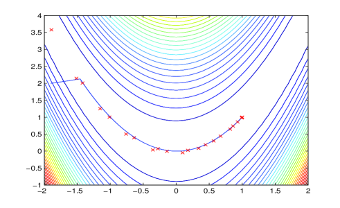
Figure 1: New algorithm searches follows the shape of the valley of Rosenbrock function.

4.3 Test of Algorithm 3.2 on CUTE problems

We also conducted test for both mNewton and Matlab optimization toolbox function fminunc against CUTE test problem set. fminunc options are set as

options = optimset(’MaxFunEvals’,1e+20,’MaxIter’,5e+5,’TolFun’,1e-20, ’TolX’,1e-10).

This setting is selected to ensure that the Matlab function fminunc will have enough iterations to converge or to fail. CUTE test problem set is downloaded from Princeton test problem collections [1]. Since CUTE test set is presented in AMPL mod-files, we first convert AMPL mod-files into nl-files so that Matlab functions can read the CUTE models, then we use Matlab functions mNewton and fminunc to read the nl-files and solve these test problems. Because the conversion software which converts mod-files to nl-files is restricted to problems whose sizes are smaller than $300$, the test is done for all CUTE unconstrained optimization problems whose sizes are less than $300$. The test uses the initial points provided by CUTE test problem set, we record the calculated objective function values, the norms of the gradients at the final points, and the iteration numbers for these testing problems. We present the test results in Table 2, and summarize the comparison of the test results as follows:

• the modified Newton function mNewton converges in all the test problems after terminate condition $\|g(x_{k})\|<10^{-5}$ is met. But for about $40\%$ of the problems, Matlab optimization toolbox function fminunc does not reduce $\|g(x_{k})\|$ to a value smaller than $0.01$. For these problems, the objective functions obtained by fminunc normally are not close to the minimum;

• for problems that both mNewton and fminunc converge, mNewton normally uses less iterations than fminunc and converges to points with smaller $\|g(x_{k})\|$ except 2 problems bard and deconvu.

Table 2: Test result for problems in CUTE [3], initial points are given in CUTE

Problem	iter	obj	gradient	iter	obj	gradient
	mNewton	mNewton	mNewton	fminunc	fminunc	fminunc
arglina	1	100.000000	0.00000000e-9	4	100.000000	0.00016620
bard	24	0.11597205	0.96811289e-5	20	0.00821487	0.1158381e-5
beale	6	0.00000000e-9	0.38908644e-9	15	0.00000024e-5	1.3929429e-5
brkmcc	2	0.16904267	0.61053106e-5	5	0.16904268	0.0454266e-5
brownal	7	0.00000000e-7	0.26143011e-7	16	0.00030509e-5	0.00010437
brownbs	8	0.00000000e-9	0.00000000e-9	11	0.00009308	15798.5950
brownden	8	85822.2016	0.00003000e-5	32	85822.2017	0.46462733
chnrosnb	46	0.00000000e-5	0.10455150e-5	98	30.0583699	10.1863739
cliff	26	0.19978661	0.10751025e-6	1	1.00159994	1.41477930
cube	28	0.00000000e-9	0.69055669e-9	34	0.79877450e-9	0.00013409
deconvu	2612	0.00242309e-5	0.99584075e-5	80	0.00031582e-3	0.1750297e-3
denschna	5	0.00000022e-5	0.29676520e-5	10	0.00000005e-5	0.1581909e-5
denschnb	5	0.00000004e-5	0.17646764e-5	7	0.00000010e-5	0.2200204e-5
denschnc	11	0.00000000e-9	0.17803850e-9	21	0.00000160e-3	0.3262483e-3
denschnd	36	0.00126578e-5	0.77956675e-5	23	45.2971677	84.5851141
denschnf	6	0.00000000e-9	0.62887898e-9	10	0.00000002e-3	0.1005028e-3
dixon3dq	1	0.00000000e-7	0.00000000e-7	20	0.00000014e-5	0.3661452e-5
eigenals	22	0.00000000e-7	0.45589372e-7	78	0.10928398e-2	0.10292633
eigenbls	62	0.00000000e-6	0.32395333e-6	91	0.34624147	0.46420894
engval2	13	0.00000001e-5	0.36978724e-7	29	0.00003953e-5	0.2799583e-3
extrosnb	1	0.00000000	0.00000000	1	0.00000000	0.00000000
fletcbv2	1	-0.5140067	0.50699056e-5	98	-0.5140067	0.1087190e-4
fletchcr	12	0.00000000e-7	0.12606909e-7	63	68.128920	160.987949
genhumps	52	0.00000003e-7	0.29148635e-7	59	0.00044932e-3	0.3167733e-3
hairy	19	20.0000000	0.00065611e-5	22	20.000000000	0.3810773e-4
heart6ls	375	0.00000000e-5	0.29136580e-5	53	0.63188192	71.9382548
helix	13	0.00000000e-9	0.31818245e-9	29	0.00000226e-5	0.4196860e-4
hilberta	1	0.00001538e-7	0.92172479e-7	35	0.02289322e-5	0.3263435e-5
hilbertb	1	0.0000004e-20	0.1267079e-12	6	0.00000021e-5	0.6542441e-5
himmelbb	7	0.0000001e-13	0.13251887e-6	6	0.00001462	0.0012511
himmelbh	4	-1.0000000	0.00108475e-6	7	-0.9999999	0.2607156e-6
humps	26	0.00000379e-6	0.27563083e-5	25	5.42481702	2.36255440
jensmp	9	124.362182	0.00480283e-5	16	124.362182	0.2897049e-5
kowosb	10	0.30750561e-3	0.31930835e-5	33	0.30750560e-3	0.0125375e-5
loghairy	23	0.18232155	0.00103147e-5	11	2.5199616136	0.0053770
mancino	4	0.00000000e-5	0.26436736e-5	9	0.00220471	1.22432874
maratosb	7	-1.0000000	0.09342000e-9	2	-0.9997167	0.03570911
mexhat	4	-0.0401000	0.00000000e-5	4	-0.0400999	0.1370395e-4
palmer1c	6	0.09759802	0.46161602e-5	38	16139.4418	655.015973
palmer2c	1	0.01442139	0.00107794e-5	60	98.0867115	33.4524366
palmer3c	1	0.01953763	0.00434478e-6	56	54.3139592	7.85183915
palmer4c	1	0.05031069	0.01265948e-6	56	62.2623173	6.67991745
palmer5c	1	2.12808666	0.00000001e-5	14	2.12808668	0.00074844
palmer6c	1	0.01638742	0.00008202e-5	43	18.0992853	0.78517164
palmer7c	1	0.60198567	0.00120838e-5	28	56.9098797	4.02685779
palmer8c	1	0.15976806	0.00013200e-5	49	22.4365812	1.31472249
powellsq	0	0	0	0	0	0
rosenbr	20	0.00000002e-5	0.10228263e-5	36	0.00000283e-5	2.6095725e-5
sineval	41	0.00000000e-8	0.24394083e-8	47	0.22121569	1.23159435
sisser	13	0.00097741e-5	0.51113540e-5	11	0.15409254e-7	0.7282671e-5
tointqor	1	1175.47222214	0.00000000000	40	1175.4722221	0.0090419e-5
vardim	19	0.00000000e-8	0.00991963e-8	1	0.22445009e-6	0.55115494
watson	13	0.15239635e-6	0.03339433e-6	90	0.00105098	0.48756107
yfitu	36	0.00000066e-6	0.10418764e-6	57	0.00439883	11.8427717

4.4 Comparison of Algorithm 3.2 to established and state-of-the-art algorithms

Most of the above problems are also used, for example in [12], to test some established and state-of-the-art algorithms. In [12], $145$ CUTEr unconstrained problems are tested against limited memory BFGS algorithm [17] (implemented as L-BFGS), a descent and conjugate gradient algorithm [14] (implemented as CG-Descent 5.3), and a limited memory descent and conjugate gradient algorithm [13] (implemented as L-CG-Descent). The sizes of most of these test problems are smaller than or equal to $300$. The size of the largest test problems in [12] is $10000$. Since our AMPL converion software does not work for problems whose sizes are larger than $300$, we compare only problems whose sizes are less than or equal to $300$. The test results obtained by algorithms descried in [17, 14, 13] are reported in [12]. In this test, we changed the stopping criterion for Algorithm 3.2 to $\|g(x)\|_{\infty}\leq 10^{-6}$ for consistency. The test results are listed in Table 3.

Table 3: Comparison of mNewtow, L-CG-Descent, L-BFGS, and CG-Descent 5.3 for problems in CUTE [3], initial points are given in CUTE

Problem	size	methods	iter	obj	gradient
arglina	200	mNewtow	1	1.000e+002	3.203e-014
		L-CG-Descent	1	2.000e+002	3.384e-008
		L-BFGS	1	2.000e+002	3.384e-008
		CG-Descent 5.3	1	2.000e+002	2.390e-007
bard	3	mNewtow	41	1.157e-001	9.765e-007
		L-CG-Descent	16	8.215e-003	3.673e-009
		L-BFGS	16	8.215e-003	3.673e-009
		CG-Descent 5.3	21	8.215e-003	1.912e-007
beale	2	mNewtow	6	4.957e-020	2.979e-010
		L-CG-Descent	15	2.727e-015	4.499e-008
		L-BFGS	15	2.727e-015	4.499e-008
		CG-Descent 5.3	18	1.497e-007	4.297e-007
brkmcc	2	mNewtow	3	1.690e-001	5.640e-013
		L-CG-Descent	5	1.690e-001	6.220e-008
		L-BFGS	5	1.690e-001	6.220e-008
		CG-Descent 5.3	4	1.690e-001	5.272e-008
brownbs	2	mNewtow	8	0.000e+000	0.000e+000
		L-CG-Descent	13	0.000e+000	0.000e+000
		L-BFGS	13	0.000e+000	0.000e+000
		CG-Descent 5.3	16	1.972e-031	8.882e-010
brownden	4	mNewtow	8	8.582e+004	3.092e-010
		L-CG-Descent	16	8.582e+004	1.282e-007
		L-BFGS	16	8.582e+004	1.282e-007
		CG-Descent 5.3	38	8.582e+004	9.083e-007
chnrosnb	50	mNewtow	46	1.885e-014	7.155e-007
		L-CG-Descent	287	6.818e-014	5.414e-007
		L-BFGS	216	1.582e-013	5.565e-007
		CG-Descent 5.3	287	6.818e-014	5.414e-007
cliff	2	mNewtow	26	1.998e-001	7.602e-008
		L-CG-Descent	18	1.998e-001	2.316e-009
		L-BFGS	18	1.998e-001	2.316e-009
		CG-Descent 5.3	19	1.998e-001	6.352e-008
cube	2	mNewtow	28	1.238e-017	1.985e-007
		L-CG-Descent	32	1.269e-017	1.225e-009
		L-BFGS	32	1.269e-017	1.225e-009
		CG-Descent 5.3	33	6.059e-015	4.697e-008
deconvu	61	mNewtow	84016	1.567e-009	9.999e-007
		L-CG-Descent	475	1.189e-008	9.187e-007
		L-BFGS	208	2.171e-010	8.924e-007
		CG-Descent 5.3	475	1.184e-008	9.078e-007
denschna	2	mNewtow	6	1.103e-023	6.642e-012
		L-CG-Descent	9	3.167e-016	3.527e-008
		L-BFGS	9	3.167e-016	3.527e-008
		CG-Descent 5.3	9	7.355e-016	4.825e-008
denschnb	2	mNewtow	6	5.550e-026	4.370e-013
		L-CG-Descent	7	3.641e-017	1.034e-008
		L-BFGS	7	3.641e-017	1.034e-008
		CG-Descent 5.3	8	4.702e-014	4.131e-007
denschnc	2	mNewtow	11	1.119e-021	1.731e-010
		L-CG-Descent	12	3.253e-019	3.276e-009
		L-BFGS	12	3.253e-019	3.276e-009
		CG-Descent 5.3	12	1.834e-001	4.143e-007
denschnd	3	mNewtow	40	3.238e-010	9.897e-007
		L-CG-Descent	47	4.331e-010	8.483e-007
		L-BFGS	47	4.331e-010	8.483e-007
		CG-Descent 5.3	45	8.800e-009	6.115e-007
denschnf	2	mNewtow	6	6.513e-022	6.281e-010
		L-CG-Descent	8	2.126e-015	6.455e-007
		L-BFGS	8	2.126e-015	6.455e-007
		CG-Descent 5.3	11	1.104e-017	6.614e-008
engval2	3	mNewtow	13	2.199e-019	3.603e-008
		L-CG-Descent	26	1.034e-016	8.236e-007
		L-BFGS	26	1.034e-016	8.236e-007
		CG-Descent 5.3	76	3.185e-014	5.682e-007
hairy	2	mNewtow	19	2.000e+001	1.149e-008
		L-CG-Descent	36	2.000e+001	7.961e-011
		L-BFGS	36	2.000e+001	7.961e-011
		CG-Descent 5.3	14	2.000e+001	1.044e-007
heart6ls	6	mNewtow	312	1.038e-023	2.993e-008
		L-CG-Descent	684	2.646e-010	5.562e-007
		L-BFGS	684	2.646e-010	5.562e-007
		CG-Descent 5.3	2570	1.305e-010	2.421e-007
helix	3	mNewtow	13	3.585e-022	3.326e-010
		L-CG-Descent	23	1.604e-015	3.135e-007
		L-BFGS	23	1.604e-015	3.135e-007
		CG-Descent 5.3	44	2.427e-013	6.444e-007
himmelbb	2	mNewtow	7	7.783e-021	1.325e-007
		L-CG-Descent	10	9.294e-013	2.375e-007
		L-BFGS	10	9.294e-013	2.375e-007
		CG-Descent 5.3	11	1.584e-013	1.084e-008
himmelbh	2	mNewtow	4	-1.000e+000	1.085e-009
		L-CG-Descent	7	-1.000e+000	2.892e-011
		L-BFGS	7	-1.000e+000	2.892e-011
		CG-Descent 5.3	7	-1.000e+000	1.381e-007
humps	2	mNewtow	37	1.695e-013	1.826e-007
		L-CG-Descent	53	3.682e-012	8.552e-007
		L-BFGS	53	3.682e-012	8.552e-007
		CG-Descent 5.3	48	3.916e-012	8.774e-007
jensmp	2	mNewtow	10	1.244e+002	2.046e-012
		L-CG-Descent	15	1.244e+002	5.302e-010
		L-BFGS	15	1.244e+002	5.302e-010
		CG-Descent 5.3	13	1.244e+002	4.206e-009
kowosb	4	mNewtow	10	3.075e-004	1.055e-007
		L-CG-Descent	17	3.078e-004	3.704e-007
		L-BFGS	17	3.078e-004	3.704e-007
		CG-Descent 5.3	66	3.078e-004	8.818e-007
loghairy	2	mNewtow	23	1.823e-001	1.880e-007
		L-CG-Descent	27	1.823e-001	1.762e-007
		L-BFGS	27	1.823e-001	1.762e-007
		CG-Descent 5.3	46	1.823e-001	7.562e-008
mancino	100	mNewtow	5	1.257e-021	4.659e-008
		L-CG-Descent	11	9.245e-021	7.239e-008
		L-BFGS	9	3.048e-021	1.576e-007
		CG-Descent 5.3	11	9.245e-021	7.239e-008
maratosb	2	mNewtow	7	-1.000e+000	9.342e-011
		L-CG-Descent	1145	-1.000e+000	3.216e-007
		L-BFGS	1145	-1.000e+000	3.216e-007
		CG-Descent 5.3	946	-1.000e+000	3.230e-009
mexhat	2	mNewtow	4	-4.010e-002	1.972e-011
		L-CG-Descent	20	-4.001e-002	4.934e-009
		L-BFGS	20	-4.001e-002	4.934e-009
		CG-Descent 5.3	27	-4.001e-002	3.014e-007
palmer1c	8	mNewtow	7	9.760e-002	6.619e-007
		L-CG-Descent	11	9.761e-002	1.254e-009
		L-BFGS	11	9.761e-002	1.254e-009
		CG-Descent 5.3	126827	9.761e-002	9.545e-007
palmer2c	8	mNewtow	1	1.442e-002	1.023e-008
		L-CG-Descent	11	1.437e-002	1.257e-008
		L-BFGS	11	1.437e-002	1.257e-008
		CG-Descent 5.3	21362	1.437e-002	5.761e-007
palmer3c	8	mNewtow	1	1.954e-002	3.958e-009
		L-CG-Descent	11	1.954e-002	1.754e-010
		L-BFGS	11	1.954e-002	1.754e-010
		CG-Descent 5.3	5536	1.954e-002	9.753e-007
palmer4c	8	mNewtow	1	5.031e-002	1.123e-008
		L-CG-Descent	11	5.031e-002	3.928e-009
		L-BFGS	11	5.031e-002	3.928e-009
		CG-Descent 5.3	44211	5.031e-002	9.657e-007
palmer5c	6	mNewtow	1	2.128e+000	1.447e-013
		L-CG-Descent	6	2.128e+000	3.749e-012
		L-BFGS	6	2.128e+000	3.749e-012
		CG-Descent 5.3	6	2.128e+000	2.629e-009
palmer6c	8	mNewtow	1	1.639e-002	7.867e-010
		L-CG-Descent	11	1.639e-002	5.520e-009
		L-BFGS	11	1.639e-002	5.520e-009
		CG-Descent 5.3	14174	1.639e-002	7.738e-007
palmer7c	8	mNewtow	1	6.020e-001	9.090e-009
		L-CG-Descent	11	6.020e-001	7.132e-009
		L-BFGS	11	6.020e-001	7.132e-009
		CG-Descent 5.3	65294	6.020e-001	9.957e-007
palmer8c	8	mNewtow	1	1.598e-001	1.099e-009
		L-CG-Descent	11	1.598e-001	2.376e-009
		L-BFGS	11	1.598e-001	2.376e-009
		CG-Descent 5.3	8935	1.598e-001	9.394e-007
rosenbr	2	mNewtow	20	2.754e-013	8.253e-007
		L-CG-Descent	34	4.691e-018	7.167e-008
		L-BFGS	34	4.691e-018	7.167e-008
		CG-Descent 5.3	37	1.004e-014	1.894e-007
sineval	2	mNewtow	41	5.590e-033	2.069e-015
		L-CG-Descent	60	1.556e-023	1.817e-011
		L-BFGS	60	1.556e-023	1.817e-011
		CG-Descent 5.3	62	1.023e-012	5.575e-007
sisser	2	mNewtow	15	3.814e-010	4.485e-007
		L-CG-Descent	6	6.830e-012	2.220e-008
		L-BFGS	6	6.830e-012	2.220e-008
		CG-Descent 5.3	6	3.026e-014	3.663e-010
tointqor	50	mNewtow	1	1.176e+003	3.197e-014
		L-CG-Descent	29	1.175e+003	4.467e-007
		L-BFGS	28	1.175e+003	7.482e-007
		CG-Descent 5.3	29	1.175e+003	4.464e-007
vardim	200	mNewtow	19	1.365e-025	7.390e-011
		L-CG-Descent	10	4.168e-019	2.582e-007
		L-BFGS	7	5.890e-025	3.070e-010
		CG-Descent 5.3	10	4.168e-019	2.582e-007
watson	12	mNewtow	16	4.202e-006	1.918e-009
		L-CG-Descent	49	1.592e-007	8.026e-007
		L-BFGS	48	9.340e-008	1.319e-007
		CG-Descent 5.3	726	1.139e-007	8.115e-007
yfitu	2	mNewtow	37	6.670e-013	2.432e-012
		L-CG-Descent	75	8.074e-010	3.910e-007
		L-BFGS	75	8.074e-010	3.910e-007
		CG-Descent 5.3	147	2.969e-011	5.681e-007

We summarize the comparison of the test results as follows:

• the modified Newton function mNewton converges in all the test problems after terminate condition $\|g(x_{k})\|_{\infty}<10^{-6}$ is met. For all problems except bard, cliff, deconvu, sisser, and vardim, the modified Newton uses fewer iterations than L-CG-Descent, L-BFGS, and CG-Descent 5.3 to converge to the minimum. Since in each iteration, mNewton needs more numerical operations, small iteration count does not mean superior efficiency, but it indicates some promising.

• For all the problems except the problem arglina, all algorithms find the same mininum. For the problem arglina, the modified Newton finds a better local minimum.

Based on these test results, we believe that the new algorithm is promising. This leads us to use the similar idea described in this paper to develop a modified BFGS algorithm which is very promising in the numerical tests.

5 Conclusions

We have proposed a modified Newton algorithm and proved that the modified Newton algorithm is globally and quadratically convergent. We show that there is an efficient way to implement the proposed algorithm. We present some numerical test results. The results show that the proposed algorithm is promising. The Matlab implementation mNewton described in this paper is available from the author.

6 acknoledgement

The author would like to thank Dr. Sven Leyffer at Atgonne National Laboratory for his suggestion of comparing the performance of Algorithm 3.2 to some established and state-of-the-art algorithms. The author is also grateful to Professor Teresa Monterio at Universidade do Minho for providing the software to convert AMPL mod-files into nl-files, which makes the test possible.

References

- [1] http://www.orfe.princeton.edu/ rvdb/ampl/nlmodels/index.html.
- [2] D.P. Bertsekas, Nonlinear Programming, Athena Scientific, Belmont, Massachusetts, 1996.
- [3] I Bongartz and A R. Conn and N. Gould and P.L. Toint, CUTE: Constrained and Unconstrained Testing Environment, ACM Transactions on Mathematical Software, Vol. 21, (1995) pp. 123-160.
- [4] H. Chen and T.K. Sarkar and J. Barule and S.A. Dianat, Adaptive spectral estimation by the conjugate gradient method, IEEE Transactions on Acousticw, Speech, and Signal Processing, Vol. 34, (1986) pp. 272-284.
- [5] A. Edelman and T.A. Arias and S.T. Smith, The geometry of algorithms with orthogonality constraints, SIAM Journal Matrix Anal. Appl., Vol. 20, (1998) pp. 303-353.
- [6] A. Edelman and S.T. Smith, On conjugate gradien-like methods for eigen-like problems, BIT, Vol. 36, (1996) pp. 1-16.
- [7] J. Fan and Y. Yuan, On the Quadratic Convergence of the Levenberg-Marquardt Method without Nonsingularity Assumption, Computing, Vol. 74, (2005) pp. 23-39.
- [8] R. Fletcher and C.M. Reeves, Function minimization by conjugate gradients, Comput. J., Vol. 7, (1964) pp. 149-154.
- [9] A. Forsgren and P. E. Gill and W. Murray, COMPUTING MODIFIED NEWTON DIRECTIONS USING A PARTIAL CHOLESKY FACTORIZATION, SIAM J. SCI. COMPUT., Vol. 16, (1995) pp. 139-150.
- [10] P. E. Gill and W. Murray, Newton-type methods for unconstrained and linearly constrained optimization, Mathematical Programming, Vol. 7, (1974) pp. 311-350.
- [11] G. H. Golub and C. F. Van Loan, Matrix Computations, The Johns Hopkins University press, Baltimore, 1989.
- [12] W. W. Hager and H. Zhang, http://www.math.ufl.edu/ hager/CG/results6.0.txt, 2012.
- [13] W. W. Hager and H. Zhang, The limited memory conjugate gradient method, http://www.math.ufl.edu/ hager/papers/CG/lcg.pdf, 2012.
- [14] W. W. Hager and H. Zhang, A new conjugate gradient method with guaranteed descent and an efficient line search, SIAM J. Optimization, Vol. 16, (2005) pp. 170-192.
- [15] MathWork, Optimization Toolbox, Boston.
- [16] J. More and D. J. Thuente, On line search algorithms with guaranteed sufficient decrease, institution=Mathematics and Computer Science Division, Argonne National Laboratory, Technical Report, MCS-P153-0590, 1990.
- [17] J. Nocedal, Updating quasi-Newton matrices with limited storage, Math. Comp., Vol. 35, (1980) pp. 773-782.
- [18] S. T. Smith, Geometric optimization methods for adaptive filtering, PhD Thesis, Harvard University, Cambridge, MA, 1993.
- [19] M.A. Townsend and G.E. Johnson, In favor of conjugate directions: A generalized acceptable-point algorithm for functin minimization, J. Franklin Inst., Vol. 306, (1978) pp. 272-284.
- [20] P. Wolfe, Convergence conditions for ascent methods, SIAM Review, Vol. 11, (1969) pp. 226-235.
- [21] P. Wolfe, Convergence conditions for ascent methods II: Some Corrections, SIAM Review, Vol. 13, (1971) pp. 185-188.
- [22] X. Yang and T. K. Sarkar and E. Arvas, A survey of conjugate gradient algorithms for solution of extreme eigen-problems of a symmetric matrix, IEEE Transactions on Acousticw, Speech, and Signal Processing, Vol. 37, (1989) pp. 1550-1556.
- [23] Y. Yang, Robust System Design: Pole Assignment Approach, PhD Thesis, University of Maryland at College Park, College Park, MD, 1996.
- [24] Y. Yang, Globally convergent optimization algorithms on Riemannian manifolds: uniform framework for unconstrained and constrained optimization, Journal of Optimization Theory and Applications, Vol. 132, (2007) pp. 245-265.
- [25] G. Zoutendijk, Nonlinear Programming, Computational Methods, editor: J. Abadie, Integer and Nonlinear Programming, Amsterdam, North Holland, (1977) pp. 37-86.