Mixing time bounds for oriented kinetically constrained spin models

Abstract.

We analyze the mixing time of a class of oriented kinetically constrained spin models (KCMs) on a $d$-dimensional lattice of $n^{d}$ sites. A typical example is the North-East model, a $0$-$1$ spin system on the two-dimensional integer lattice that evolves according to the following rule: whenever a site’s southerly and westerly nearest neighbours have spin $0$, with rate one it resets its own spin by tossing a $p$-coin, at all other times its spin remains frozen. Such models are very popular in statistical physics because, in spite of their simplicity, they display some of the key features of the dynamics of real glasses. We prove that the mixing time is $O(n\log n)$ whenever the relaxation time is $O(1)$. Our study was motivated by the “shape” conjecture put forward by G. Kordzakhia and S.P. Lalley.

Keywords: North-East model, kinetically constrained spin models, mixing time.

AMS subject classifications: 60J10,60J27,60J28.

1. Introduction

Kinetically constrained spin models (KCMs) are interacting $0$-$1$ particle systems, on general graphs, which evolve with a simple Glauber dynamics described as follows. At every site $x$ the system tries to update the occupancy variable (or spin) at $x$ to the value $1$ or $0$ with probability $p$ and $q$ respectively. However the update at $x$ is accepted only if the current local configuration satisfies a certain constraint, hence the models are “kinetically constrained”. It is always assumed that the constraint at site $x$ does not to depend on the spin at $x$ and therefore the product Bernoulli($p$) measure $\pi$ is the reversible measure. Constraints may require, for example, that a certain number of the neighbouring spins are in state $0$, or more restrictively, that certain preassigned neighbouring spins are in state $0$ (e.g. the children of $x$ when the underlying graph is a rooted tree).

The main interest in the physical literature for KCMs (see e.g. [Ritort] for a review) stems from the fact that they display many key dynamical features of real glassy materials: ergodicity breaking transition at some critical value $q_{c}$, huge relaxation time for $q$ close to $q_{c}$, dynamic heterogeneity (non-trivial spatio-temporal fluctuations of the local relaxation to equilibrium) and aging, just to mention a few. Mathematically, despite their simple definition, KCMs pose very challenging and interesting problems because of the hardness of the constraint, with ramifications towards bootstrap percolation problems [Spiral], combinatorics [CDG, Valiant:2004cb], coalescence processes [FMRT-cmp, FMRT] and random walks on upper triangular matrices [Peres-Sly]. Some of the mathematical tools developed for the analysis of the relaxation process of KCMs [CMRT] proved to be quite powerful also in other contexts such as card shuffling problems [Bhatnagar:2007tr] and random evolution of surfaces [PietroCaputo:2012vl].

In this paper we focus on oriented KCMs on a $d$-dimensional lattice, $d\;\geqslant\;2$, with $n^{d}$ sites, in particular on their mixing time. A prototypical model belonging to the above class of KCMs is the North-East model in two dimensions (see e.g. [Kordzakhia:2006] and [CMRT]) for which the constraint at any given site $x$ requires the south and west neighbours of $x$ to be empty in order for a flip at $x$ to occur. In order to avoid trivial irreducibility issues the south-westerly most spin is unconstrained and sites outside the upper quadrant are treated as fixed zeros.

With $p_{c}$ the percolation threshold for oriented percolation in two dimensions (see e.g. [Durrett:1984tm]), it was proved in [CMRT] that for all $p<p_{c}$ the relaxation time of the North-East process is $O(1)$ while it becomes $\Omega(e^{cn})$, for some $c>0$, when $p>p_{c}$. At $p=p_{c}$ the relaxation time is expected to have a poly$(n)$ growth. Consider now the North-East model in the first quadrant of ${\mathbb{Z}}^{2}$. In [Kordzakhia:2006] it was conjectured that, for $p<p_{c}$ and starting from all $1$’s, the influence region $R_{t}$, defined as the union of all unit squares around those sites which have flipped at least once by time $t$, has a definite limiting shape $S\subset{\mathbb{R}}^{2}$ in the sense that a.s. $\frac{R_{t}}{t}\to S$ as $t\to\infty$. Since the North-East process is neither monotone or additive (see [Liggett1]), the usual tools to prove a shape theorem do not apply in this case.

The above conjecture implies that, for $p<p_{c}$, the influence coming from the unconstrained spin at the South-West corner propagates at a definite linear rate as it does in the East model [Blondel:2012wb], the one dimensional analog of the model (for background see [Aldous, CMRT, SE1]). In particular the mixing time of the model should grow linearly in $n$ (the linear size of the system). However in dimension $d\geq 2$ the analysis of the propagation of influence is quite delicate because of the many paths along which it can occur (see [Valiant:2004cb] for combinatorial results in this direction).

In this paper we prove that the mixing time is $O(n\log n)$ as long as the spectral gap of the process is $\Omega(1)$. Our technique bares some similarities to those employed in [Caputo:2011dv] to analyse the Glauber dynamics of biased plane partitions.

2. Models and Results

2.1. Setting and notation

We consider a class of $0$-$1$ interacting particle systems on finite subsets $\Lambda$ of the integer lattice ${\mathbb{Z}}^{d}$, reversible with respect to the product measure $\pi:=\prod_{x\in\Lambda}\pi_{x}$, where $\pi_{x}$ is the Bernoulli$(p)$ measure.

The $d$-dimensional cube of linear size $n$ (which contain $n^{d}$ points) will be denoted by

$$\Lambda_{n}:=\left([1,n]\times\ldots\times[1,n]\right)\cap{\mathbb{Z}}^{d}\,.$$

The standard basis vectors in ${\mathbb{Z}}^{d}$ are denoted $\mathbf{e}_{1}=(1,\ldots,0)$, $\mathbf{e}_{1}=(0,1,\ldots,0),\ldots$, $\mathbf{e}_{d}=(0,\ldots,1)$. For $x\in\Lambda_{n}$ we write $x_{j}$ for the component of $x$ in the direction $\mathbf{e}_{j}$.

The set of probability measures on the finite state space $\Omega_{n}=\{0,1\}^{\Lambda_{n}}$ is denoted by $\mathcal{P}(\Omega_{n})$. Elements of $\Omega_{n}$ will be denoted by the small greek letters $\sigma,\eta,\ldots$ and $\sigma_{x}$ will denote the spin at the vertex $x$.

We denote the $i$-th level hyperplane in $\Lambda_{n}$ by $\mathcal{H}_{i}=\{x\in\Lambda_{n}:\sum_{j=1}^{d}x_{j}=i\}$ (see Fig. 1). The set of sites on and below this hyperplane will be written $\mathcal{U}_{i}=\{x\in\Lambda_{n}:\sum_{j=1}^{d}x_{j}\;\leqslant\;i\}$. For each $\sigma\in\Omega_{n}$ we write $\sigma^{(i)}$ for the restriction of $\sigma$ to $\mathcal{U}_{i}$, and $\sigma_{\mathcal{H}_{i}}$ for the restriction of $\sigma$ to $\mathcal{H}_{i}$. Similarly, for any probability measure $\nu\in\mathcal{P}(\Omega_{n})$, we write $\nu^{(i)}$ for the marginal of $\nu$ on $\Omega^{(i)}:=\{0,1\}^{\mathcal{U}_{i}}\subset\Omega_{n}$.

For any vertex $x\in\Lambda_{n}$ we also let (see Fig. 1 Right)

$$\mathcal{K}_{x}^{*} =\Big{\{}y\in{\mathbb{Z}}^{d}:y=x-\sum_{i=1}^{d}\alpha_{i}\mathbf{e}_{i},\ \alpha_{i}\in\{1,0\}\Big{\}}\setminus\{x\}$$

$$\mathcal{K}_{x} =\Big{\{}y\in{\mathbb{Z}}^{d}:\exists\ i=1,\dots,d\text{ such that }y=x-\mathbf{e}_{i}\Big{\}}\,.$$

  

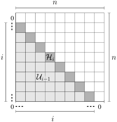
(a)

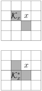
(b)

Figure 1. Left: The the lattice $\Lambda_{n}$ in two dimensions, $d=2$. The sets $\mathcal{H}_{i}$ and $\mathcal{U}_{i-1}$ are shown in dark grey and light grey respectively. Right: The constraining neighbourhoods, $\mathcal{K}_{x}$ and $\mathcal{K}_{x}^{*}$, of a vertex $x$ in two dimensions, shown in dark grey.

Definition 2.1 (constraints).

Let $x_{*}=(1,\dots,1)$ be the south-west corner of $\Lambda_{n}$. Consider a collection $\{\mathcal{C}_{x}\}_{x\in\Lambda_{n}}$ of constraining neighborhoods such that

$$\mathcal{C}_{x_{*}}=\emptyset,\qquad\text{and}\qquad\emptyset\neq\mathcal{C}_{x}\subset K_{x}^{*}\cap\Lambda_{n},\quad x\neq x_{*}.$$

Let

$$c_{x}(\sigma):=\begin{cases}\prod_{y\in\mathcal{C}_{x}}(1-\sigma_{y})&\text{if $x\neq x_{*}$}\\ 1&\text{$x=x_{*}$.}\end{cases}$$ (2.1)

We then say that the constraint at site $x$ is satisfied by the configuration $\sigma$ if $c_{x}(\sigma)=1$. In words, the constraint at $x$ is satisfied if all the spin in $\mathcal{C}_{x}$ are $0$. Note that $x_{*}$ is unconstrained.

2.2. Oriented KCMs and main result

We give a general definition of the process to include a large class of directed KCMs, such as the North-East model and higher dimensional analogues. For constraining neighborhoods $\{\mathcal{C}_{x}\}_{x\in\Lambda_{n}}$ we define the associated directed KCM by the following graphical construction. To each $x\in\Lambda_{n}$ we associate a mean one Poisson process and, independently, a family of independent Bernoulli$(p)$ random variables $\{s_{x,k}:k\in\mathbb{N}\}$. The occurrences of the Poisson process associated to $x$ will be denoted by $\{t_{x,k}:k\in\mathbb{N}\}$. We assume independence as $x$ varies in $\Lambda_{n}$. The probability measure will be denoted by ${\mathbb{P}}^{\Lambda_{n}}$. Notice that ${\mathbb{P}}^{\Lambda_{n}}$-almost surely all the occurrences $\{t_{x,k}\}_{k\in\mathbb{N},x\in\Lambda_{n}}$ are different.

Given $\eta\in\Omega_{n}$ we construct a continuous time Markov chain $\{\eta(s)\}_{s\;\geqslant\;0}$ on the probability space above, starting from $\eta$ at $t=0$, according to the following rules. At each time $t_{x,n}$ the site $x$ queries the state of its own constraint $c_{x}$ (see (2.1)). If and only if the constraint is satisfied ($c_{x}=1$) then $t_{x,n}$ is called a legal ring and the configuration resets its value at site $x$ to the value of the corresponding Bernoulli variable $s_{x,n}$.

The above construction gives rise to an irreducible, continuous time Markov chain, reversible w.r.t. $\pi$, with generator

$$\mathcal{L}_{n}f(\sigma)=\sum_{x\in\Lambda_{n}}c_{x}(\sigma)[\pi_{x}(f)-f(\sigma)]\,,$$ (2.2)

where $\pi_{x}$ denotes the conditional mean $\pi(f\mid\{\sigma_{y}\}_{y\neq x})$. Irreducibility follows because we can invade $\Lambda_{n}$ with $0$’s starting from the unconstrained corner $x_{*}$.

Using a standard percolation argument [Liggett2, Durrett] together with the fact that the constraints $\{c_{x}\}_{x\in\Lambda_{n}}$ are uniformly bounded and of finite range, it is not difficult to see that the graphical construction can be extended without problems also to the infinite volume case.

For an initial distribution $\nu$ at $t=0$ the law and expectation of the process will be denoted by ${\mathbb{P}}_{\nu}$ and $\mathbb{E}_{\nu}$ respectively. In the sequel, we will write $\nu_{t}$ for the distribution of the chain at time $t$,

$$\nu_{t}[\eta]:={\mathbb{P}}_{\nu}(\eta(t)=\eta).$$

If $\nu$ is concentrated on a single configuration $\eta$ we will write ${\mathbb{P}}_{\eta}(\cdot)$. Note that, for each $i=1,\dots,n$, the same graphical construction can be used to define the process on $\Omega^{(i)}$ whose law is denoted by ${\mathbb{P}}_{\nu}^{(i)}(\cdot)$.

It follows from the graphical construction, and the fact that the constraints are oriented, that given an $i\in\{1\ldots,n\}$ the evolution in $\mathcal{U}_{i}$ is not influenced by the evolution above $\mathcal{U}_{i}$. In particular, for any $\eta\in\Omega_{n}$ and any event $\mathcal{A}$ in the $\sigma$-algebra generated by $\{\eta_{x}(s)\}_{s\;\leqslant\;t,x\in\mathcal{U}_{i}}$,

$${\mathbb{P}}_{\eta}(\mathcal{A})={\mathbb{P}}_{\eta^{(i)}}^{(i)}(\mathcal{A})\,.$$ (2.3)

In fact the same holds for any subset $U\subset\Lambda_{n}$ with monotone surface, i.e. $x-\mathbf{e}_{i}\in U$ whenever $x\in U$ and $x-\mathbf{e}_{i}\in\Lambda_{n}$, for each $i\in\{1,\ldots,d\}$.

We finish this section with definitions of the spectral gap and mixing time of the process.

Definition 2.2 (spectral gap).

The spectral gap, $\lambda^{(n)}$, of the infinitesimal generator (2.2) is the smallest positive eigenvalue of $-\mathcal{L}_{n}$ , and is given by the variational principle

$$\lambda^{(n)}:=\inf_{\begin{subarray}{c}f:\Omega_{n}\to{\mathbb{R}}\\ f\neq\textrm{const}\end{subarray}}\frac{\mathcal{D}_{n}(f)}{{\rm Var}_{n}(f)},$$ (2.4)

where $\mathcal{D}_{n}(f)=-\pi\left(f\mathcal{L}_{n}f\right)$ is the Dirichlet form of the process.

Definition 2.3 (Mixing time).

The mixing time is defined in the usual way as

$$T_{\rm mix}^{(n)}=\inf\{t>0:\sup_{\nu\in\mathcal{P}(\Omega_{n})}\left\|\nu_{t}-\pi\right\|_{\rm TV}\;\leqslant\;1/4\}\,,$$ (2.5)

where $\|\cdot\|_{\rm TV}$ denotes the total variation distance.

Remark 2.4.

It follows from [CMRT, Theorem 4.1] that there exists $0<p_{0}<1$ such that $\inf_{n}\lambda^{(n)}>0$ whenever $p<p_{0}$. For the North-East model $p_{0}$ coincides with the oriented percolation threshold. Moreover, for any $p\in(0,1)$, one has $1/\lambda^{(n)}\;\leqslant\;T_{\rm mix}^{(n)}\;\leqslant\;c\,n^{d}/\lambda^{(n)}$ (see e.g. [Levin2008]).

Our main result reads as follows.

Theorem 2.5.

Assume $\inf_{n}\lambda^{(n)}>0$, then

$$C\,n\;\leqslant\;T_{\rm mix}^{(n)}\;\leqslant\;C^{\prime}\,n\log n$$ (2.6)

for some $C,C^{\prime}>0$ independent of $n$.

Remark 2.6.

In the case of maximal constraints, i.e. $\mathcal{C}_{x}=\mathcal{K}_{x}^{*}\cap\Lambda_{n}$, inserting the indicator of the configuration identically equal to $1$ as a test function in the logarithmic Sobolev inequality [Saloff] shows that the logarithmic Sobolev constant $\alpha^{(n)}$ of the generator (2.2) is $O(1/n^{d})$. Therefore, if

$$T^{(n)}_{2}:=\inf\{t\geq 0:\ \sup_{\nu}\operatorname{Var}\left(\frac{\nu_{t}}{\pi}\right)\;\leqslant\;1/4\},$$

then for a universal constants $c>0$ and a constant $c^{\prime}>0$ depending only on $p$,

$$T^{(n)}_{2}\geq\frac{c}{\alpha^{(n)}}\geq c^{\prime}n^{d},$$

where the first inequality follows from [Saloff, Corollary 2.2.7]. This observation shows that oriented models in ${\mathbb{Z}}^{d}$ can be quite different from oriented models on rooted $k$-regular trees. In the latter case it was recently proved [Martinelli:2012tp] that both the mixing time $T_{\rm mix}^{(n)}$ and $T^{(n)}_{2}$ grow linearly in the depth $n$ of the tree whenever the relaxation time $1/\lambda^{(n)}$ is $O(1)$.

3. Proof of theorem 2.5

Proof of the lower bound.

The lower bound on the mixing time is quite straightforward using finite speed of propagation. Define $\tau^{*}$ as the first time the spin at site $x^{*}:=(n,\ldots,n)$ is $0$, and denote the configuration of all $1$’s by $\mathds{1}$. Using results in [O, PS] there exists $c>0$ such that

$${T_{\textrm{mix}}^{(n)}}\;\geqslant\;c{\mathbb{E}}_{\mathds{1}}\bigl{[}\tau^{*}\bigr{]}\;\geqslant\;\frac{c\,n}{2}{\mathbb{P}}_{\mathds{1}}\bigl{(}\tau^{*}\geq n/2\bigr{)}.$$ (3.1)

Clearly the event $\tau^{*}<n/2$ requires the existence of a path $\gamma=\{x_{*}=x^{(0)},x^{(1)},\dots,x^{(\ell)}=x^{*}\}$ and times $t_{0}<t_{1}<\dots<t_{\ell}<n/2$ such that, for any $i\;\leqslant\;\ell$, $x^{(i)}\in\mathcal{C}_{x^{(i+1)}}$ and $t_{i}$ is a legal ring for $x^{(i)}$. Standard Poisson large deviations show that the probability of the above event is $o(1)$ as $n\to\infty$. ∎

Proof of the upper bound.

The proof of the upper bound is based on an iterative scheme. For $i\;\leqslant\;n$, we find some time, $\Delta_{i}=O(\log(i))$, such that if the initial measure $\nu$ has marginal $\nu^{(i-1)}$ equal to $\pi^{(i-1)}$ on $\Omega^{(i-1)}$ (i.e. below the hyperplane $\mathcal{H}_{i}$), then after time $\Delta_{i}$ the marginal $\nu^{(i)}$ is very close to the equilibrium marginal $\pi^{(i)}$. This is the content of Lemma 3.1. Then, starting from an arbitrary initial measure, we can iterate the above result using the triangle inequality for the variation distance and propagate the error.

Lemma 3.1 (Mixing time for a single diagonal.).

There exists $c=c(q,d)>0$ such that, for any initial measure $\nu$ with marginal on $\Omega^{(i-1)}$ equal to $\pi^{(i-1)}$,

$$\left\|\nu^{(i)}_{t}-\pi^{(i)}\right\|_{\rm TV}\;\leqslant\;\epsilon\quad\textrm{for all}\quad t\;\geqslant\;c\,\log(i/\epsilon)\ .$$

Before proving Lemma 3.1 let us recall a useful characterisation of the total variation distance (see for example [Levin2008]),

$$\left\|\nu-\pi\right\|_{\rm TV}=\frac{1}{2}\sup_{\|f\|_{\infty}\;\leqslant\;1}\left|\nu(f)-\pi(f)\right|\,,$$

where $\|f\|_{\infty}$ denotes the sup-norm.

Proof of Lemma 3.1.

Fix $i\;\leqslant\;n$ and a function $f$ depending only on the spin configuration in $\mathcal{U}_{i}$ and such that $\|f\|_{\infty}\;\leqslant\;1$. Without loss of generality assume $\pi(f)=0$. Given an initial measure $\nu$ with marginal $\pi^{(i-1)}$ on $\Omega^{(i-1)}$ it follows from (2.3) that $\nu_{t}^{(i-1)}=\pi^{(i-1)}$ for all $t\;\geqslant\;0$. Moreover, conditioned on the history $\{\sigma^{(i-1)}(s)\}_{s\;\leqslant\;t}$ in $\mathcal{U}_{i-1}$, the spins $\{\sigma_{x}(t)\}_{x\in\mathcal{H}_{i}}$ on the hyperplane $\mathcal{H}_{i}$ evolve independently from each other. Each one goes to equilibrium with rate one during the intervals of time in which its constraint $c_{x}$ is satisfied and stays fixed otherwise. In particular, conditioned on having had a legal ring at each $x\in\mathcal{H}_{i}$ before time $t$, the distribution of $\sigma_{\mathcal{H}_{i}}(t)$ is $\pi$. These simple observations gives rise to an upper-bound on the expectation of $f$ at time $t$ as follows.

Let $\tau^{(i)}$ be the first time there has been at least one legal ring on each $x\in\mathcal{H}_{i}$. Following the argument above we have,

$$\left|{\mathbb{E}}_{\nu}\left[f\left(\sigma^{(i)}(t)\right)\right]\right|= \left|\ {\mathbb{E}}_{\nu}\left({\mathbb{E}}_{\nu}\left[f\left(\sigma^{(i)}(t)\right)\mid\big{\{}\sigma^{(i-1)}(s)\big{\}}_{s\;\leqslant\;t}\right]\right)\right|$$

$$\;\leqslant\; \left|\ {\mathbb{E}}_{\nu}\left({\mathbb{E}}_{\nu}\left[f\left(\sigma^{(i)}(t)\right)\mathds{1}_{\{\tau^{i}<t\}}\mid\big{\{}\sigma^{(i-1)}(s)\big{\}}_{s\;\leqslant\;t}\right]\right)\right|+$$

$$+\left|\ {\mathbb{E}}_{\nu}\left({\mathbb{E}}_{\nu}\left[f\left(\sigma^{(i)}(t)\right)\mathds{1}_{\{\tau^{i}\geq t\}}\mid\big{\{}\sigma^{(i-1)}(s)\big{\}}_{s\;\leqslant\;t}\right]\right)\right|$$

$$\;\leqslant\; \left|\ {\mathbb{E}}_{\nu}\left(\pi_{\mathcal{H}_{i}}\left(f\right){\mathbb{P}}_{\nu}\left(\tau^{i}<t\mid\big{\{}\sigma^{(i-1)}(s)\big{\}}_{s\;\leqslant\;t}\right)\right)\right|+$$

$$+\left|\ {\mathbb{E}}_{\nu}\left({\mathbb{E}}_{\nu}\left[f\left(\sigma^{(i)}(t)\right)\mathds{1}_{\{\tau^{i}\geq t\}}\mid\big{\{}\sigma^{(i-1)}(s)\big{\}}_{s\;\leqslant\;t}\right]\right)\right|$$

$$\;\leqslant\; 2{\mathbb{E}}_{\pi}\left[{\mathbb{P}}_{\nu}\left(\tau^{i}\geq t\mid\big{\{}\sigma^{(i-1)}(s)\big{\}}_{s\;\leqslant\;t}\right)\right].$$

In the second inequality above we used the strong Markov property together with the observation that the distribution of $\sigma_{\mathcal{H}_{i}}(t)$ conditioned on $\{\tau^{(i)}<t\}$ and $\big{\{}\sigma^{(i-1)}(s)\big{\}}_{s\;\leqslant\;t}$ is $\pi$. In the third inequality we used the fact that ${\mathbb{E}}_{\nu}\left(\pi_{\mathcal{H}_{i}}(f)\right)=\pi(f)=0$.

To bound the final term above we denote the number of rings of the Poisson clock at site $x$ during the set $B\subset[0,t]$ by $N_{x}(B)=\lvert\{t_{x,k}\}_{k\;\geqslant\;0}\cap B\rvert$, and we define the set of legal times at site $x$ before $t$ as $\mathcal{G}(x,t):=\{s<t:c_{x}(\sigma(s))=1\}$. By construction, for $x\in\mathcal{H}_{i}$ the set $\mathcal{G}(x,t)$ depends only on $\left\{\sigma_{y}(s)\right\}_{s\;\leqslant\;t},\ y\in\mathcal{C}_{x}$. Using the notation above,

$${\mathbb{P}}_{\nu}\left(\tau^{(i)}\geq t\mid\big{\{}\sigma^{(i-1)}(s)\big{\}}_{s\;\leqslant\;t}\right)\;\leqslant\;\sum_{x\in\mathcal{H}_{i}}{\mathbb{P}}\left(N_{x}(\mathcal{G}(x,t))=0\mid\big{\{}\sigma^{(i-1)}(s)\big{\}}_{s\;\leqslant\;t}\right).$$

By construction $N_{x}(\mathcal{G}(x,t))$ is a Poisson random variable of mean $|\mathcal{G}(x,t)|$. Thus

$$\sum_{x\in\mathcal{H}_{i}}{\mathbb{P}}\left(N_{x}(\mathcal{G}(x,t))=0\mid\big{\{}\sigma^{(i-1)}(s)\big{\}}_{s\;\leqslant\;t}\right)=\sum_{x\in\mathcal{H}_{i}}e^{-|\mathcal{G}(x,t)|}.$$

In conclusion,

$$\left|{\mathbb{E}}_{\nu}\left[f\left(\sigma^{(i)}(t)\right)\right]\right| \;\leqslant\;2\sum_{x\in\mathcal{H}_{i}}{\mathbb{E}}_{\pi}\left[e^{-|\mathcal{G}(x,t)|}\right]\;\leqslant\;2i^{d-1}\max_{y\in\Lambda_{n}}{\mathbb{E}}_{\pi}\left[e^{-|\mathcal{G}(y,t)|}\right].$$

We estimate ${\mathbb{E}}_{\pi}\left[e^{-|\mathcal{G}(y,t)|}\right]$ using a Feynman-Kac approach (a similar method has been used to bound the persistence function in [CMRT]). The total time that site $y$ satisfies its constraints is

$$|\mathcal{G}(y,t)|=\int_{0}^{t}c_{y}\left(\sigma(s)\right)ds.$$

On $L^{2}(\pi)$ we define the self adjoint operator $H:=\mathcal{L}-V$ with $V(\sigma):=c_{y}(\sigma)$. The Feynman-Kac formula allows us to rewrite the expectation ${\mathbb{E}}_{\pi}\left[e^{-\int_{0}^{t}V}\right]$ as $\left\langle\mathbf{1},e^{tH}\mathbf{1}\right\rangle_{\pi}$ (where $\left\langle\cdot,\cdot\right\rangle_{\pi}$ denotes the inner-product in $L^{2}(\pi)$). Thus, if $\beta_{y}$ is the supremum of the spectrum of $H$ we have

$${\mathbb{E}}_{\pi}\left[e^{-|\mathcal{G}(y,t)|}\right]\;\leqslant\;e^{t\beta_{y}}\ .$$ (3.2)

In order to complete the proof of the Lemma it remains to show that $\beta_{y}<0$.

We decompose each $L^{2}(\pi)$-norm one function $\phi$ in the domain of $H$ as $\phi=\alpha\mathbf{1}+g$, for some mean zero function $g$. So $\left\langle\mathbf{1},g\right\rangle_{\pi}=0$ and $\alpha^{2}+\langle g,g\rangle_{\pi}=1$. Then,

$$\left\langle\phi,H\phi\right\rangle=\left\langle g,\mathcal{L}g\right\rangle_{\pi}-\alpha^{2}\left\langle\mathbf{1},V\mathbf{1}\right\rangle_{\pi}-2\alpha\left\langle\mathbf{1},Vg\right\rangle_{\pi}-\left\langle g,Vg\right\rangle_{\pi}$$ (3.3)

We proceed by bounding $\left\langle\phi,H\phi\right\rangle_{\pi}$. Using (3.3) together with the Cauchy-Schwarz inequality we get

$$\left\langle\phi,H\phi\right\rangle \;\leqslant\;-\lambda^{(n)}\,\langle g,g\rangle_{\pi}-q^{d}\Big{(}\alpha^{2}+2{\mathbb{E}}_{\pi}\left(g\mid V=1\right)\alpha+{\mathbb{E}}_{\pi}\left(g^{2}\mid V=1\right)\Big{)}$$

$$\;\leqslant\;-\delta\,\lambda^{(n)}-q^{d}\Big{(}|\alpha|-{\mathbb{E}}_{\pi}\left(g^{2}\mid V=1\right)^{1/2}\Big{)}^{2}$$

$$\;\leqslant\;-\delta\,\lambda^{(n)}$$

where $\delta=1-\alpha^{2}$. Again from (3.3), dropping the last term on the right hand side and applying the Cauchy-Schwarz inequality we get

$$\left\langle\phi,H\phi\right\rangle \;\leqslant\;-\lambda^{(n)}\ \langle g,g\rangle_{\pi}-\alpha^{2}q^{d}+2|\alpha|\left(\langle g,g\rangle_{\pi}q^{d}(1-q^{d})\right)^{1/2}$$

$$\;\leqslant\;(\delta-1)q^{d}+2\left(\delta q^{d}(1-q^{d})\right)^{1/2}.$$

Thus

$$\beta_{y}\;\leqslant\;-c_{0}(q):=\min\left(-\delta\,\lambda^{(n)},(\delta-1)q^{d}+2\left(\delta q^{d}(1-q^{d})\right)^{1/2}\right).$$

Finally we observe that $c_{0}(q)>0$ because

$$(\delta-1)q^{d}+2\left(\delta q^{d}(1-q^{d})\right)^{1/2}\;\leqslant\;-\frac{q^{d}}{2}\quad\textrm{if}\quad\delta\;\leqslant\;\frac{2(1-\sqrt{1-q^{d}})-q^{d}}{4q^{d}}.$$

In conclusion

$$\left|{\mathbb{E}}_{\nu}\left[f\left(\sigma^{(i)}(t)\right)\right]\right|\;\leqslant\;2i^{d}e^{-c_{0}(q)t}\;\leqslant\;\epsilon,$$

for $t\;\geqslant\;c\log(i/\epsilon)$ for some $c=c(d,q)$. ∎

We now prove Theorem 2.5 by iterating the previous Lemma and propagating the error. We use the following iterative scheme

$$t_{i}=t_{i-1}+\Delta_{i},\quad t_{0}=0\,,$$ (3.4)

where $\Delta_{i}(\epsilon)=\frac{1}{c}\log(i^{3}/\epsilon)$ with $c$ as in the Lemma. We now show by induction that starting from an arbitrary initial distribution $\nu$

$$2\left\|\nu^{(i)}_{t}-\pi^{(i)}\right\|_{\rm TV}\;\leqslant\;\hat{\epsilon}_{i}:=\epsilon\sum_{j=1}^{i}\frac{1}{j^{2}}\quad\textrm{for all}\quad t\;\geqslant\;t_{i}\ .$$ (3.5)

The case $i=1$ (3.5) is an immediate consequence of the fact that the corner $x_{*}=(1,\dots,1)$ goes to equilibrium with rate one. Assume (3.5) holds for all $i\;\leqslant\;k-1$. It is clear that $\min_{\sigma}\nu_{t}(\sigma)>0$ for any $t>0$, so that we may define an auxiliary probability measure $\mu$ with marginal $\mu^{(k-1)}=\pi^{(k-1)}$ by

$$\mu[\sigma]:=\pi^{(k-1)}\left[\sigma^{(k-1)}\right]\,\nu_{t_{k-1}}\left[\sigma\thinspace|\thinspace\sigma^{(k-1)}\right].$$

Fix a function $f$ depending only on the configuration in $\mathcal{U}_{k}$ with $\|f\|_{\infty}\;\leqslant\;1$. Again, without loss of generality, assume $\pi(f)=0$. Then

$$\Big{|}{\mathbb{E}}_{\nu}\left[f\left(\sigma(t_{k})\right)\right]\Big{|} =\Big{|}{\mathbb{E}}_{\nu_{t_{k-1}}}\left[f\left(\sigma(\Delta_{k})\right)\right]\Big{|}$$

$$\;\leqslant\;\Big{|}{\mathbb{E}}_{\nu_{t_{k-1}}}\left[f\left(\sigma(\Delta_{k})\right)\right]-{\mathbb{E}}_{\mu}\left[f\left(\sigma(\Delta_{k})\right)\right]\Big{|}+\frac{\varepsilon}{k^{2}}\,.$$ (3.6)

where we used the Markov property in the first line and Lemma 3.1 together with the triangle inequality in the second line. The two measures $\mu$ and $\nu_{t_{k-1}}$ have the same marginal on $\mathcal{H}_{k}$, so we may reduce the remaining term to something that can be dealt with using the inductive hypothesis as follows. For any $\eta\in\Omega^{(k-1)}$ let

$$F\left(\eta\right):={\mathbb{E}}_{\nu_{t_{k-1}}}\left[f\left(\sigma(\Delta_{k})\right)\thinspace|\thinspace\sigma^{(k-1)}=\eta\right].$$

Clearly $\|F\|_{\infty}\;\leqslant\;1$, so by the definition of $\mu$ and the inductive hypothesis (3.5),

$$\Big{|}{\mathbb{E}}_{\nu_{t_{k-1}}}\left[f\left(\sigma(\Delta_{k})\right)\right]-{\mathbb{E}}_{\mu}\left[f\left(\sigma(\Delta_{k})\right)\right]\Big{|}=\left|\nu_{t_{k-1}}\left(F\right)-\pi\left(F\right)\right|\;\leqslant\;\hat{\varepsilon}_{k-1}\,.$$

In conclusion the r.h.s. of (3) is bounded from above by

$$\Big{|}{\mathbb{E}}_{\nu}\left[f\left(\sigma(t_{k})\right)\right]\Big{|} =\hat{\varepsilon}_{k-1}+\frac{\varepsilon}{k^{2}}=\hat{\varepsilon}_{k}\,.$$

Since $\mathcal{U}_{2n-1}\supseteq\Lambda_{n}$, it follows that

$$2\left\|\nu_{t}-\pi\right\|_{\rm TV}\;\leqslant\;\hat{\epsilon}_{2n-1}=\epsilon\sum_{j=1}^{2n-1}\frac{1}{j^{2}}\;\leqslant\;2\varepsilon\quad\textrm{for all}\quad t\;\geqslant\;t_{2n-1}$$

and

$$t_{2n-1}=\sum_{j=1}^{2n-1}\Delta_{j}\;\leqslant\;\frac{1}{c}\int_{0}^{2n}\log(x^{3}/\epsilon)dx\;\leqslant\;c^{\prime}n\log(n)$$

for some $c^{\prime}>0$. ∎

4. Acknowledgments

We would like to thank O. Blondel for a very careful reading of the paper.