Abstract

We demonstrate in this paper that the effect of object shift in an elliptical, astigmatic Gaussian beam does not affect the optimal fractional orders used to reconstruct the holographic image of a particle or another opaque object in the field. Simulations and experimental results are presented.

OCIS codes: 090.0090, 070.0070

1 Introduction

Digital in-line holography (DIH) is widely used in microscopy for biological applications [1, 2], in 3D Holographic Particle Image Velocimetry (HPIV) for fluid mechanics studies[3] and in refractometry [4]. In most theoretical DIH studies, the optical systems or the objects used, for example particles, are considered to be centered on the optical axis [5, 6]. Nevertheless, in many practical applications, the systems and objects are not necessarily centered. This is not a problem under plane wave illumination. But more and more studies involve a diverging beam, or astigmatic beams directly obtained at the output of fibered laser diodes or astigmatic laser diodes. The position of the object in the beam becomes particularly relevant. To reconstruct the image of an object, a reconstruction parameter must be determined in order to find the best focus plane. For wavelet transformation, the parameter is the scale factor [7]. For Fresnel transformation, the parameter is the distance $z$ from the object to the quadratic sensor plane [8] and for the fractional Fourier transformation, the parameters are the fractional orders [10, 9]. It is considered here that the same parameter can be used for all positions of the object. Recently, an analytical solution of scalar diffraction of an elliptical and astigmatic Gaussian beam (EAGB) by a centered opaque disk under Fresnel approximation has been proposed. By using the fractional Fourier transformation, a good particle image reconstruction is obtained [11]. However, there are no recent publications in DIH theory demonstrating that reconstruction parameter is constant for all transverse positions of the object in the field of the beam. This is, however, particularly important if we want to develop wide-angle metrologies.

In this publication, the aim is to demonstrate that the same fractional orders can be used to reconstruct an image of the particle whatever its position in the field of the beam. We exhibit the effect of the Gaussian beam on the reconstructed image. In the first part of this publication, the model of the analytical solution of scalar diffraction of an EAGB by a centered opaque disk is revisited to take into account a decentered object. In the second part, the definition of the fractional Fourier transformation is recalled and this transformation is used to reconstruct the image of the particle. It is in this part that we demonstrate that the same orders can be used. Finally, we propose to illustrate our results by simulations and experimental results.

2 In-line Holography with an elliptic and astigmatic Gaussian beam

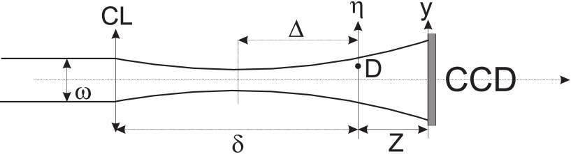
Fig. 1: Numerical and experimental optical set-up.

The basic idea in DIH is to record by a CCD camera the intensity distribution of the diffraction pattern of an object illuminated by a continuous or pulsed wave [12]. Figure (1) represents the numerical and experimental set-up where all parameters are identified. The incident Gaussian beam of diameter $\omega$ crosses a plano-convex cylindrical lens. This cylindrical lens acts only in the $\eta$-axis. Its focal length is equal to $f_{\eta}=200mm$. After propagation in free space, the elliptical and astigmatic Gaussian beam illuminates an opaque particle. In the plane of the object, the beam widths along the $\xi$-axis and $\eta$-axis are defined by $\omega_{\xi}$ and $\omega_{\eta}$. The wavefront curvatures of the astigmatic beam are denoted by $R_{q}$ with $q=\xi,\eta$. The CCD camera is located at a distance $z$ from the opaque particle.

The basic model to describe the intensity distribution of the diffracted beam by an object recorded by the CCD camera is the integral of Kirchhoff-Fresnel given by the scalar integral for the complex amplitude $A$ in the quadratic sensor plane:

$$A=\frac{\exp(i\frac{2\pi}{\lambda}z)}{i\lambda z}\int_{\mathbb{R}^{2}}E_{T}(\xi,\eta)\,\exp\left(\frac{i\pi}{\lambda z}\left[(\xi-x)^{2}+(\eta-y)^{2}\right]\right)\,d\xi d\eta,$$ (1)

in which $E_{T}(\xi,\eta)$ is the product of the optical incident beam, denoted $E(\xi,\eta)$, by the spatial transmittance of the shifted opaque 2D-object, denoted $1-T(\xi-\xi_{0},\eta-\eta_{0})$. The quadratic sensor records the intensity defined by $|A|^{2}$. If we consider that the function $E_{T}$ is the product of an elliptic and astigmatic Gaussian beam by an opaque disk of diameter $D$, then

$$E_{T}(\xi,\eta)=\underbrace{\exp\left[c_{\xi}\xi^{2}+c_{\eta}\eta^{2}\right]}_{=E(\xi,\eta)}\cdot\underbrace{[1-T(\xi-\xi_{0},\eta-\eta_{0})]}_{shifted\,\,object}.$$ (2)

The complex coefficients $c_{\xi}$ and $c_{\eta}$ are

$$c_{\xi}=-\frac{1}{\omega_{\xi}^{2}}-i\frac{\pi}{\lambda R_{\xi}},\quad c_{\eta}=-\frac{1}{\omega_{\eta}^{2}}-i\frac{\pi}{\lambda R_{\eta}},$$ (3)

For an opaque disk centered at the origin O, the transmittance function $T(\xi,\eta)$ in the object plane is:

$$T(\xi,\eta)=\begin{cases}1,&\text{$0<\sqrt{\xi^{2}+\eta^{2}}$ $<$ $D/2$},\\ 1/2,&\text{$0<\sqrt{\xi^{2}+\eta^{2}}$ $=$ $D/2$},\\ 0,&\text{$\sqrt{\xi^{2}+\eta^{2}}$ $>$ $D/2>0$}.\end{cases}$$ (4)

¿From Eqs. (1) and (2), the expression for $A(x,y)$ can split into two integral terms, denoted $A_{1}$ and $A_{2}$ so that:

$$A(x,y)=\frac{\exp(i\frac{2\pi}{\lambda}z)}{i}\left[A_{1}-A_{2}\right].$$ (5)

The expression of these two terms is given in the Appendix (A). The complex amplitude $A_{1}$ represents the propagation of the incident beam without diffraction by the particle and $A_{2}$ contains the diffraction by a pinhole of diameter $D$. After some development detailed in the Appendix (A), the expression of $A_{2}$ becomes:

$$A_{2}=\frac{\pi D^{2}}{\lambda z}\exp\left[\Phi(\xi_{0},\eta_{0})\right]\cdot\exp\left(ic_{z}\left[(x-\xi_{0})^{2}+(y-\eta_{0})^{2}\right]\right)\cdot\sum_{k=0}^{\infty}(-i)^{k}\varepsilon_{k}\,T_{k}(r,\gamma)\cos(2k\theta),$$ (6)

with

$$T_{k}(r,\gamma)=\sum_{p=0}^{\infty}\beta_{2k+2p}^{2k}(\delta)V_{2k+2p}^{2k}(r,\gamma),$$ (7)

and

$$V_{2k+2p}^{2k}(r,\gamma)=\exp(i\gamma/2)\sum_{m=0}^{\infty}(2m+1)i^{m}j_{m}\small{(\gamma/2)}\cdot\sum_{l=\max(0,m-2k-p,p-m)}^{m+p}(-1)^{l}\omega_{ml}\frac{J_{2k+2l+1}(r)}{r}.$$ (8)

The coefficients $\omega_{ml}$ are given explicitly in [11] and [14]. Finally, the expression of $A_{1}$ contains only the characteristics of the incident beam and $A_{2}$ contains a shifted linear chirp function linked to the object shift in the EAGB. The previous function is modulated by a series of Bessel functions which constitutes the envelope of the amplitude distribution of $A_{2}$.

A similar expression has been established in [11] for a particle located on the axis of the beam, i.e. $\xi_{0}=0$ and $\eta_{0}=0$. This last expression is more general and can be applied to a particle located everywhere in the field of the beam.

In our previous study, we demonstrated that a fractional-order Fourier transformation allows a particle located on the axis of the beam to be reconstructed. Unfortunately, the expression of the diffraction pattern (and particularly $A_{2}$) is so complex that it cannot be proved theoretically that a digital (or optical) reconstruction leads effectively to an opaque disk function. The demonstration is empirical. In addition, nothing proves that the fractional orders used for the reconstruction would be appropriate if the object were shifted transversely.

In the next developments, we will thus prove theoretically that the reconstruction leads effectively to the object. We will then demonstrate that the reconstruction process is successful whatever the transversal position of the particle in the field of the beam. In addition, we show that the same fractional orders have to be applied. We will thus be able to conclude that reconstruction is possible for a whole wide-field object or wide particle field in such a beam.

Now, to obtain the desired accuracy, we should analyze the number of terms necessary in the series over $k$ in Eq. (6) and over $p$ in Eq. (7). The series which should be analyzed are in Eq.(8). The first upper bound that is relevant here is [14, 15, 16]

$$\left|j_{m}\small{\left(\frac{\gamma}{2}\right)}\right|\leq\frac{1}{(2m+1)^{1/2}}\,\min\left(1,\left(\frac{\pi}{2}\right)^{1/2}\frac{|\gamma/4|^{m}}{m!}\right).$$ (9)

The coefficients $\omega_{ml}$ verify $\omega_{ml}\geq 0$ and $\sum_{l}\omega_{ml}=1$, so the $\omega$’s are completely innocent. Using the bound (9) for the function $\left|j_{m}\small{\left(\frac{\gamma}{2}\right)}\right|$ requires a rough estimate of the variable $\gamma$. In practical experiments, we have $D\approx 10^{-4}m$, $\lambda\approx 10^{-6}m$, $z\approx 10^{-1}m$, $R_{q}\approx 0.5\cdot 10^{-1}$ then $\gamma\approx 0.785\cdot 10^{-1}+0.816\cdot 10^{-3}i$. The right-hand side of Eq. (9) is less than $0.142\cdot 10^{-1}$ for $m\geq 1$. The second upper bound we use concerns the Bessel functions $J_{2k+2l+1}$. From [17], 9.1.62 on p.362 and [14] we obtain:

$$\left|\frac{J_{2k+2l+1}(r)}{r}\right|\leq\min\left(1,\frac{1}{2}\frac{|r|^{2k+2l}\exp(|r|^{2})}{(2k+2l+1)!}\right).$$ (10)

The evaluation of the accuracy concerns the product of the left-hand side of Eqs. (9) and (10):

$$\left|j_{m}\small{\left(\frac{\gamma}{2}\right)}\right|\left|\frac{J_{2k+2(m+p)+1}(r)}{r}\right|.$$ (11)

With the previous values, all the quantities in (11) are less than $0.142\cdot 10^{-1}$ for all $(k,p,m)\geq 1$. Thus, we only consider the case where $k=p=m=0$. In conclusion, the function $V_{0}^{0}(r,\gamma)$ is given with good accuracy by:

$$V_{0}^{0}(r,\gamma)\simeq\exp(i\gamma/2)j_{0}\small{(\gamma/2)}\frac{J_{1}(r)}{r}.$$ (12)

Note that this result is true if the object is far from the beam waist. The amplitude $A_{2}$ then becomes

$$A_{2}=\frac{\pi D^{2}}{2\lambda z}\beta_{0}^{0}(\delta)\exp\left[\Phi(\xi_{0},\eta_{0})\right]\exp\left(ic_{z}\left[(x-\xi_{0})^{2}+(y-\eta_{0})^{2}\right]\right)\cdot V_{0}^{0}(r,\gamma).$$ (13)

2.A Intensity distribution of the diffraction pattern

The intensity distribution of the diffraction pattern in the quadratic sensor plane, denoted $I$, is evaluated from the Eqs. (5), (13) and (36) in the following way:

$$I=A\overline{A}=\left[A_{1}-A_{2}\right]\left[\overline{A_{1}}-\overline{A_{2}}\right]=\left[|A_{1}|^{2}+|A_{2}|^{2}\right]-2\,\Re\left\{A_{1}\overline{A_{2}}\right\},$$ (14)

where the overhead bar denotes the complex conjugate, $\Re$ denotes the real part. Thus, the intensity distribution recorded by the CCD sensor is described by the Eq. (14). As one sees from the form of $I$, the first and second terms, i.e., $|A_{1}|^{2}$ and $|A_{2}|^{2}$, do not generate interference fringes with a linear instantaneous frequency, denoted $f_{i}(x)$, in the CCD plane, i.e. [18]:

$$f_{i}(x)=\frac{1}{2\pi}\frac{\partial\varphi(x)}{\partial x}=\frac{1}{2\pi}\frac{\partial\arg(|A_{1,2}|)}{\partial x}=0.$$ (15)

But the third term exhibits a phase which is composed of a constant and a linear instantaneous frequency. This fact is important because the fractional Fourier transform is an effective operator for analyzing a signal containing a linear instantaneous frequency (linear chirp functions). From Eq. (14) we write

$$A_{1}\overline{A_{2}}=|A_{1}\overline{A_{2}}|\exp\left[i\arg\left(A_{1}\overline{A_{2}}\right)\right],$$ (16)

where $\arg\left(A_{1}\overline{A_{2}}\right)=\phi-\phi_{0}$ with

$$\phi=c_{z}\left(x^{2}(M_{\xi}-1)+y^{2}(M_{\eta}-1)\right)+2c_{z}\left(x\xi_{0}+y\eta_{0}\right)-\arg\left(\frac{J_{1}(r)}{r}\right),$$ (17)

and

$$\phi_{0}=\frac{\Re(\gamma)}{2}+\Im(\Phi(\xi_{0},\eta_{0}))+\arg\left(j_{0}\small{\left(\frac{\gamma}{2}\right)}\right)+\arg\left(\beta_{0}^{0}(\delta)\right)-\arg\left(K_{\xi}K_{\eta}\right),$$ (18)

where $\Im$ represent the imaginary part of a complex number. The first term in (17) yields a quadratic phase and the second term yields a linear phase. Remember that the aim of the reconstruction by means of FRFT is precisely to analyze a linear chirp.

To give two different examples, it is necessary to fix the values of the parameters $(\omega_{\xi},\omega_{\eta})$, $(R_{\xi},R_{\eta})$ and $(D,\lambda,z)$.

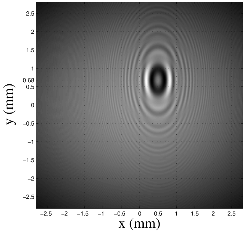
Fig. 2: Diffraction pattern with , $\omega_{\xi}=7mm$, $\omega_{\eta}=1.75mm$, $R_{\xi}=\infty$, $R_{\eta}=-50mm$, $D=150\textmu m$, $\lambda=632.8nm$, $z=120mm$, $\delta=250mm$, $\xi_{0}=0.5mm$ and $\eta_{0}=0.2mm$.

In the first case, the values are defined by $(7mm,1.75mm)$ for the beam waists, $(-\infty,-50mm)$ for the wave’s curvatures and the diameter $D$ of the particle is equal to $150\textmu m$ and located at $120mm$ from the CCD sensor. The wavelength of the laser beam is $632.8nm$. The distance between the cylindrical lens and the particle is $\delta=250mm$. The particle is shifted from the origin by $(\xi_{0},\eta_{0})=(0.5mm,0.2mm)$. Figure (2) illustrates the diffraction pattern which is recorded by the camera. Note that the shift of the diffraction pattern $(x_{0},y_{0})$ observed in the camera plane is not equal to the object shift $(\xi_{0},\eta_{0})$. If the particle is considered far from the beam waist then we have the formula:

$$y_{0}=\frac{\mid\Delta\mid\pm z}{\mid\Delta\mid}\,\,\eta_{0}.$$ (19)

The sign of $z$ depends on the position of the particle compared with the position of the waist. If the particle is after the waist, the sign is positive. If it is in front of the waist, the sign is negative. Along $x$-axis, the parameter $\Delta$ is infinite so that in the plane of the camera $x_{0}=\xi_{0}=0.5mm$ and along $y$-axis, $\Delta=50mm$ thus $y_{0}=0.68mm$.

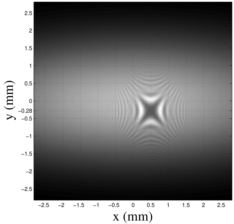
Fig. 3: Diffraction pattern with , $\omega_{\xi}=7mm$, $\omega_{\eta}=1.75mm$, $R_{\xi}=\infty$, $R_{\eta}=-50mm$, $D=150\textmu m$, $\lambda=632.8nm$, $z=120mm$, $\delta=150mm$, $\xi_{0}=0.5mm$ and $\eta_{0}=0.2mm$.

Now, in the second case, the values are defined by $(7mm,1.75mm)$ for the beam waists, $(-\infty,50mm)$ for the wave’s curvatures and the diameter $D$ of the particle is equal to $150\textmu m$ and located at $z=120mm$ from the CCD sensor. The distance between the cylindrical lens and the particle is $\delta=150mm$. The particle is shifted from the origin by $(\xi_{0},\eta_{0})=(0.5mm,0.2mm)$. Figure (3) illustrates the diffraction pattern which is recorded by the camera. In the plane of the camera, $x_{0}=\xi_{0}=0.5mm$, $\Delta=50mm$ thus, from Eq. (19), it leads to $y_{0}=-0.28mm$. The diffraction pattern changes from elliptical fringes to hyperbolic fringes. These diffraction patterns will be used to reconstruct the image of the particle by FRFT.

3 Fractional Fourier transformation analysis of in-line holograms

3.A Two-dimensional Fractional Fourier transformation

FRFT is an integral operator that has various application in signal and image processing. Its mathematical definition is given in Ref. [20, 19, 21]. The two-dimensional fractional Fourier transformation of order $a_{x}$ for $x$-cross-section and $a_{y}$ for $y$-cross-section with $0\leq|\alpha_{x}|\leq\pi/2$ and $0\leq|\alpha_{y}|\leq\pi/2$, respectively, of a 2D-function $I(x,y)$ is defined as (with $\alpha_{p}=\frac{a_{p}\pi}{2}$)

$$\mathscr{F}_{\alpha_{x},\alpha_{y}}[I(x,y)](x_{a},y_{a})=\int_{\mathbb{R}^{2}}N_{\alpha_{x}}(x,x_{a})\,N_{\alpha_{y}}(y,y_{a})I(x,y)\,dx\,dy,$$ (20)

where the kernel of the fractional operator is defined by

$$N_{\alpha_{p}}(x,x_{a})=C(\alpha_{p})\exp\left(i\pi\frac{x^{2}+x_{a}^{2}}{s_{p}^{2}\tan\alpha_{p}}\right)\exp\left(-\frac{i2\pi x_{a}x}{s_{p}^{2}\sin\alpha_{p}}\right),$$ (21)

and

$$C(\alpha_{p})=\frac{\exp(-i(\frac{\pi}{4}\textrm{sign}(\sin\alpha_{p})-\frac{\alpha_{p}}{2}))}{|s_{p}^{2}\sin\alpha_{p}|^{1/2}}\,.$$ (22)

Here $p=x,y$. Generally, the parameter $s_{p}$ is considered as a normalization constant. It can take any value. In our case, its value is defined from the experimental set-up according to [22]

$$s_{p}^{2}=N_{p}\cdot\delta_{p}^{2}.$$ (23)

This definition is presented in the Appendix C. $N_{p}$ is the number of samples along the $x$ and $y$ axes in both spatial $I(x,y)$ and fractional domains. The constant $\delta_{p}$ is the sampling period along the two previous axes of the image. In our case the number of samples and the sampling period are the same along both axes, so that the parameters $s_{p}$ are equal to $s$. The energy-conservation law is ensured by the coefficient $C(\alpha_{p})$ which is a function of the fractional order. One of the most important FRFT feature is its ability to transform a linear chirp into a Dirac impulse. Let $g(x)=\exp\left(i\pi\chi x^{2}\right)$ the chirp function to be analyzed. If we consider $\frac{1}{\chi}=-\tan\alpha$, and using the fact that:

$$\lim_{\varepsilon\rightarrow 0}\frac{1}{\sqrt{i\pi\varepsilon}}\exp\left(-\frac{x^{2}}{i\varepsilon}\right)=\delta(x),$$ (24)

then the FRFT of optimal order $\alpha$ of $g(x)$ can be written as:

$$\mathscr{F}_{\alpha}\left[g(x)\right]=\delta(x_{a}).$$ (25)

Finally, by choosing the adequate value of the fractional order, a pure linear chirp function can be transformed into a delta Dirac distribution.

3.B Reconstruction: optimal fractional orders

To reconstruct the image of the particle, the FRFT of the diffraction pattern (Eq.(14)) must be calculated:

$$\begin{split}\mathscr{F}_{\alpha_{x},\alpha_{y}}[I]&=\mathscr{F}_{\alpha_{x},\alpha_{y}}\left[|A_{1}|^{2}\right]-\mathscr{F}_{\alpha_{x},\alpha_{y}}\left[2|A_{1}\overline{A_{2}}|\cos(\phi-\phi_{0})\right]+\mathscr{F}_{\alpha_{x},\alpha_{y}}\left[|A_{2}|^{2}\right]\end{split}$$ (26)

The terms $|A_{1}|^{2}$ and $|A_{2}|^{2}$ do not contain a linear chirp, so they do not have any effect on the optimal fractional order to be determined. But the second term, denoted $S_{t}$ contains a linear chirp. It will be considered for the image reconstruction of the particle. By noting that $2\cos(\phi-\phi_{0})=\exp(-i(\phi-\phi_{0}))+\exp(i(\phi-\phi_{0}))$, the second term of Eq. (26) becomes :

$$\mathscr{F}_{\alpha_{x},\alpha_{y}}\left[2|A_{1}\overline{A_{2}}|\cos(\phi-\phi_{0})\right]=\exp\left(i\pi\frac{x_{a}^{2}}{s^{2}\tan\alpha_{x}}\right)\exp\left(i\pi\frac{y_{a}^{2}}{s^{2}\tan\alpha_{y}}\right)\left\{I_{-}+I_{+}\right\}$$ (27)

with

$$I_{\pm}=C(\alpha_{x})C(\alpha_{y})\iint_{\mathbb{R}^{2}}\left|A_{1}\overline{A_{2}}\right|\exp\left[i\left(\phi_{a}\pm(\phi-\phi_{0})\right)\right]\exp\left[-\frac{2i\pi}{s^{2}}\left(\frac{x_{a}x}{\sin\alpha_{x}}+\frac{y_{a}y}{\sin\alpha_{y}}\right)\right]dxdy$$ (28)

The quadratic phase term of the FRFT is denoted by $\phi_{a}=\frac{\pi}{s^{2}}\left(x^{2}\cot\alpha_{x}+y^{2}\cot\alpha_{y}\right)$. Let us recall that the FRFT allows us to analyze a linear chirp. Thus, if the fractional orders check the following conditions

$$\frac{\pi\cot\alpha_{x}^{opt}}{s^{2}}=c_{z}(M_{x}-1),\quad\quad\frac{\pi\cot\alpha_{y}^{opt}}{s^{2}}=c_{z}(M_{y}-1),$$ (29)

then, the FRFT of $I_{-}$ is no more than a classical Fourier transformation according to

$$I_{-}=\chi\cdot\mathcal{F}\left[\frac{J_{1}(r)}{r}\cdot\exp\left(-\frac{\pi}{\lambda z}\rho^{\mathrm{T}}N\rho\right)\right](u,v),$$ (30)

with $\chi=\frac{\pi D^{2}}{2\lambda z}C(\alpha_{x})C(\alpha_{y})K_{\xi}K_{\eta}\exp\left[\Phi(\xi_{0},\eta_{0})\right]\beta_{0}^{0}(\delta)\exp\left(i\frac{\gamma}{2}\right)j_{0}\small{\left(\frac{\gamma}{2}\right)}$. The operator $\mathcal{F}$ is the 2D-Fourier transformation. The spatial frequencies $u$ and $v$ are equal to:

$$u=\frac{x_{a}}{s^{2}\sin(\alpha_{x}^{opt})}+\frac{c_{z}\xi_{0}}{\pi}\quad\quad v=\frac{y_{a}}{s^{2}\sin(\alpha_{y}^{opt})}+\frac{c_{z}\eta_{0}}{\pi}$$ (31)

As the Fourier transform of the product of two functions is equal to the convolution of their transforms then

$$I_{-}=\chi\cdot\mathcal{F}\left[\frac{J_{1}(r)}{r}\right]\ast\mathcal{F}\left[\exp\left(-\frac{\pi}{\lambda z}\rho^{\mathrm{T}}N\rho\right)\right],$$ (32)

Remember here that the variables $\rho$ and $r$ pertain to the same coordinates $(x,y)$. With the shift theorem for the Fourier transform, the Hankel transform and the discontinuous Weber-Schafheitlin integral in [[17]], 11.4.42 on p.487, we have:

$$\mathcal{F}\left[\frac{J_{1}(r)}{r}\right]=2\pi\left(\frac{\lambda z}{\pi D}\right)^{2}\exp\left[-i2\pi(uX_{0}+vY_{0})\right]\times\begin{cases}1,&\text{$0<\sqrt{u^{2}+v^{2}}$ $<$ $\frac{D/2}{\lambda z}$},\\ 1/2,&\text{$0<\sqrt{u^{2}+v^{2}}$ = $\frac{D/2}{\lambda z}$},\\ 0,&\text{$\sqrt{u^{2}+v^{2}}$ > $\frac{D/2}{\lambda z}>0$},\end{cases}$$ (33)

with $X_{0}=\xi_{0}\left(1-ic_{\xi}/c_{z}\right)$ and $Y_{0}=\eta_{0}\left(1-ic_{\eta}/c_{z}\right)$. The function defined by the right-hand side of Eq. (33), with spatial coordinates $(x_{a},y_{a})$, has the aperture of the pinhole with diameter equal to the diameter $D$ of the opaque particle. We have thus demonstrated our result: reconstruction with a FRFT leads exactly to the object. In addition, shifting the object does not modify the fractional order. This point is important because in the case of a particle field, a single fractional order couple along the $x-$ axis and $y-$ axis is necessary to reconstruct the particle image. If one wishes to determine the shift of the diffraction patterns in the $(x_{a},y_{a})$-plane, the coordinates that should be considered are:

$$\left(s^{2}(u-\frac{c_{z}\xi_{0}}{\pi})\tan\alpha_{x}^{opt},s^{2}(v-\frac{c_{z}\eta_{0}}{\pi})\tan\alpha_{y}^{opt}\right)$$ (34)

This correction is necessary because the fractional Fourier transformation is not invariant by translation: a space-shift in the spatial domain will lead to both frequency-shift and phase-shift in the FRFT domain. The shift rule of the FRFT is expressed as:

$$\mathscr{F}_{\alpha}[f(x-b)](u)=\exp\left(i\pi b^{2}\sin\alpha\cos\alpha\right)\exp\left(-i2\pi bu\sin\alpha\right)\mathscr{F}_{\alpha}[f(x)](u-b\cos\alpha)$$ (35)

Note that the nature of the Gaussian beam implies that the reconstructed image of the object is convolved by a 2D Gaussian function. The sign of the object function (opaque object with a luminous background) is retrieved by applying an inversion of $I_{-}$ that is realized by the minus in front of the second term of Eq. (26).

3.C Numerical experiments

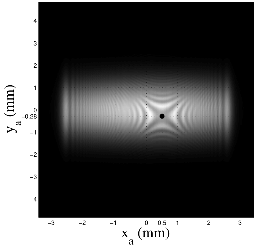
Fig. 5: Fractional Fourier transform of the diffraction pattern with $a_{x}^{opt}=-0.564$ and $a_{y}^{opt}=0.664$.

The simulations of the particle image reconstruction are realized from the diffraction patterns illustrated by the Figs. (2) and (3). The diffraction patterns consist of a $512\times 512$ array of $11\textmu m\times 11\textmu m$ size pixels. Consider the diffraction pattern presented in Fig. (2) and produced by a particle of $D=150\textmu m$ in diameter located at $z=120mm$. The optimal fractional orders obtained from Eq. (29) are $a_{x}^{opt}=-0.564$ and $a_{y}^{opt}=-0.850$. The image of the reconstructed image is shown in Fig. (4). In this representation, the squared modulus of the FRFT, i.e. $|\mathscr{F}_{\alpha_{x},\alpha_{y}}[I]|^{2}$, is taken. The shape of the particle image is not modified: the width of the Gaussian function in the Eq.(32) is greater than the diameter $D$ of the particle (typically $679\textmu m$ along x-cross axis and $490\textmu m$ along y-cross axis). Now, the reconstruction of the particle image from the diffraction pattern illustrated by Fig. (3), is realized by a fractional Fourier transformation of optimal orders $a_{x}^{opt}=-0.564$ and $a_{y}^{opt}=0.664$. Figure (5) illustrates the result of the reconstruction. In both cases (Fig.(4) and Fig.(5)) reconstruction by FRFT is successful. Note that we have checked that the apertures resulting from Eq. (32) and the image of the reconstructed particle give the same diameter $D$.

3.D Experimental results

As the reconstruction process is successful whatever the transversal position of the particle in the field of the beam, for the same fractional orders we can now carry out a reconstruction for a wide-field object.

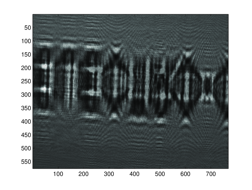
Fig. 6: Diffraction pattern of the word ”ELECTRO”.

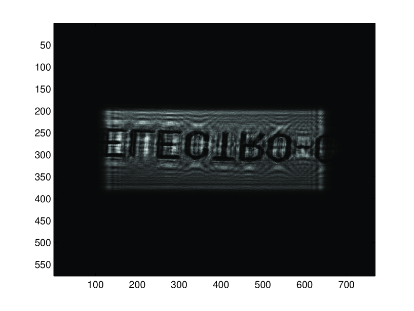
Fig. 7: Fractional Fourier transform of the diffraction pattern with $a_{x}^{opt}=0.505$ and $a_{y}^{opt}=-0.785$.

The previous theoretical developments and numerical experiments have been tested by using an RS-3 standard reticle (Malvern Equipment). This reticle is an optical glass plate with a pattern of the word ”ELECTRO” photographically deposited on the surface. The word ”ELECTRO” spread over $6.5mm$. The reticle is located at $\delta\approx 156mm$ from the cylindrical lens (CL). The distance $z$ between the CCD camera and the reticle is approximatively equal to $117mm$. The opaque word ”ELECTRO” is in front of the waist of the beam. The intensity distribution of the EAGB diffracted by the word ”ELECTRO” is shown in Fig. (6). The image of the word ”ELECTRO” is reconstructed by the fractional Fourier transformation. Fractional orders have been adjusted to obtain the best contrast between the reconstructed ”ELECTRO” word and the background. Thus doing, the approximate orders are $a_{x}^{opt}=0.505$ and $a_{y}^{opt}=-0.785$. The image of Fig. (7) shows that two previous orders allow all parts of the image of the object to be reconstructed. Note that the word is reversed along the $y-$axis. This is due to the Gouy phase shift of a Gaussian beam that propagates from $-\infty$ to $+\infty$ through the focus point. In this case, the phase shift predicted is $\pi$.

4 Conclusion

The effect of a transversal object shift in an elliptical, astigmatic Gaussian beam does not affect the optimal fractional orders required to reconstruct the image of a particle or any other opaque object in the field. In this publication an analytical model has been developed to prove this. In this development, an opaque particle is considered. Experimental result presented by the recording and reconstruction of the word ”ELECTRO” show that our method works, even when the object is spread out over the whole image field.

Appendix A Appendix A : Expression of the terms $A_{1}$ and $A_{2}$

A.A Expression for the amplitude distribution $A_{1}$

The development of integral $A_{1}$ has been given in a previous paper by [11] :

$$A_{1}=K_{\xi}K_{\eta}\exp\left(-\frac{\pi}{\lambda z}\rho^{\mathrm{T}}N\rho\right)\exp\left(i\frac{\pi}{\lambda z}\rho^{\mathrm{T}}M\rho\right)$$ (36)

where $\rho^{\mathrm{T}}$ represents the vector $(x\quad y)$ and the factors $K_{q}$ with $q=\xi,\eta$ in Eq.(36) are defined by

$$K_{q}=\left[\frac{\frac{\pi\omega_{q}^{2}}{\lambda z}}{1+i\frac{\pi\omega_{q}^{2}}{\lambda z}\left(\frac{z}{R_{q}}-1\right)}\right]^{1/2}$$ (37)

and the diagonal matrices $N$ and $M$ by

$$N=\left(\begin{array}[]{cc}N_{x}&0\\ 0&N_{y}\\ \end{array}\right),\quad\quad M=\left(\begin{array}[]{cc}M_{x}&0\\ 0&M_{y}\\ \end{array}\right),$$ (38)

with

$$N_{q}=\pi\,\frac{\frac{\omega_{q}^{2}}{\lambda z}}{1+\pi^{2}\frac{\omega_{q}^{4}}{(\lambda z)^{2}}\left(\frac{z}{R_{q}}-1\right)^{2}}\quad\quad\textrm{,}\quad\quad M_{q}=1+\pi^{2}\,\,\frac{\,\frac{\omega_{q}^{4}}{(\lambda z)^{2}}\left(\frac{z}{R_{q}}-1\right)}{1+\pi^{2}\frac{\omega_{q}^{4}}{(\lambda z)^{2}}\left(\frac{z}{R_{q}}-1\right)^{2}}.$$ (39)

A.B Expression for the amplitude distribution $A_{2}$

To develop the second integral of $A_{2}$, involving the product of $E(\xi,\eta)$ and $T(\xi-\xi_{0},\eta-\eta_{0})$, i.e.:

$$A_{2}=\frac{\exp\left[\frac{i\pi}{\lambda z}(x^{2}+y^{2})\right]}{\lambda z}\int_{\mathbb{R}^{2}}E(\xi,\eta)T(\xi-\xi_{0},\eta-\eta_{0})\exp\left[\frac{i\pi}{\lambda z}(\xi^{2}+\eta^{2})\right]\exp\left[-i\frac{2\pi}{\lambda z}(x\xi+y\eta)\right]\,d\xi d\eta,$$ (40)

we first replace $\xi$ by $\xi+\xi_{0}$ and $\eta$ by $\eta+\eta_{0}$ and get:

$$A_{2}=\frac{\exp\left[\frac{i\pi}{\lambda z}(x^{2}+y^{2})\right]}{\lambda z}\int_{\mathcal{D}}E(\xi+\xi_{0},\eta+\eta_{0})\exp\left[\frac{i\pi}{\lambda z}((\xi+\xi_{0})^{2}+(\eta+\eta_{0})^{2})\right]\times\\ \exp\left[-i\frac{2\pi}{\lambda z}(x(\xi+\xi_{0})+y(\eta+\eta_{0}))\right]\,d\xi d\eta.$$ (41)

The domain $\mathcal{D}$ must be defined as the disk with center $0$ and diameter $D$. By considering that $c_{z}=\pi/(\lambda z)$ and by restating $A_{2}$ in cylindrical coordinates as follows: $\xi=D\sigma\cos(\varphi)/2$ and $\eta=D\sigma\sin(\varphi)/2$ for the object plane, we obtain:

$$A_{2}=\frac{D^{2}}{4\lambda z}\exp\left[c_{\xi}\xi_{0}^{2}+c_{\eta}\eta_{0}^{2}+ic_{z}\left[(x-\xi_{0})^{2}+(y-\eta_{0})^{2}\right]\right]\cdot\\ \int_{0}^{1}\int_{0}^{2\pi}\exp\left[i\gamma\sigma^{2}\right]\exp\left[i\delta\sigma^{2}\cos(2\varphi)\right]\exp\left[ia\sigma\cos\varphi+ib\sigma\sin\varphi\right]\,\sigma d\sigma d\varphi$$ (42)

with

$$\begin{array}[]{l}\displaystyle\gamma=\frac{D^{2}}{4}\,c_{z}-i\frac{D^{2}}{8}\,(c_{\xi}+c_{\eta}),\quad\quad\delta=i\,\frac{D^{2}}{8}\,(c_{\eta}-c_{\xi}),\\[11.38092pt] \displaystyle a=Dc_{z}\left[\xi_{0}\left(1-ic_{\xi}/c_{z}\right)-x\right],\quad\quad b=Dc_{z}\left[\eta_{0}\left(1-ic_{\eta}/c_{z}\right)-y\right].\\[11.38092pt] \end{array}$$ (45)

By writing:

$$a\cos\varphi+b\sin\varphi=r\cos(\varphi-\theta)$$ (46)

for which we have the condition

$$a=r\cos\theta,\quad\quad b=r\sin\theta$$ (47)

with complex $r$ and $\theta$. This representation is discussed in some detail in Appendix B. By means of the following equalities in [[17]], 9.1.41 - 9.1.45:

$$\exp\left[i\delta\sigma^{2}\cos\left(2\varphi+2\theta\right)\right]=J_{0}\left(\delta\sigma^{2}\right)+2\sum_{k=1}^{+\infty}i^{k}J_{k}\left(\delta\sigma^{2}\right)\cos 2k(\varphi+\theta),$$ (48)

and

$$\frac{1}{2\pi}\int_{0}^{2\pi}\exp(in\theta)\exp[ix\cos\theta]d\theta=i^{n}J_{n}(x),$$ (49)

the expression of $A_{2}$ becomes:

$$A_{2}=\frac{\pi D^{2}}{\lambda z}\exp\left[\Phi(\xi_{0},\eta_{0})\right]\cdot\exp\left(ic_{z}\left[(x-\xi_{0})^{2}+(y-\eta_{0})^{2}\right]\right)\cdot\sum_{k=0}^{\infty}(-i)^{k}\varepsilon_{k}\,T_{k}(r,\gamma)\cos(2k\theta),$$ (50)

with $\varepsilon_{k}=1/2$ if $k=0$ and $1$ otherwise. The parameter denoted $\Phi(\xi_{0},\eta_{0})$ is equal to $\left[c_{\xi}\xi_{0}^{2}+c_{\eta}\eta_{0}^{2}\right]$. The function $T_{k}(r,2\gamma)$ is defined as:

$$T_{k}(r,\gamma)=\sum_{p=0}^{\infty}\beta_{2k+2p}^{2k}(\delta)V_{2k+2p}^{2k}(r,\gamma),$$ (51)

where the coefficients $\beta_{2k+2p}^{2k}$ are given by the analytical development of $T_{k}$ in Appendix of [[11]]. Recall here that the expression of $V_{2k+2p}^{2k}(r,\gamma)$ is:

$$V_{2k+2p}^{2k}(r,\gamma)=\exp(i\gamma/2)\sum_{m=0}^{\infty}(2m+1)i^{m}j_{m}\small{(\gamma/2)}\cdot\sum_{l=\max(0,m-2k-p,p-m)}^{m+p}(-1)^{l}\omega_{ml}\frac{J_{2k+2l+1}(r)}{r}.$$ (52)

The coefficients $\omega_{ml}$ is given explicitly in [[11]] and [[14]].

Appendix B Appendix B : Elaboration of condition (47)

With $u=a+ib$, $v=a-ib$, we should find $\tau$ and $\omega=\exp(i\theta)$ such that

$$\tau\omega=u,\quad\quad\tau/\omega=v$$ (53)

Assume that $u\neq 0$, $v\neq 0$, and write $u=r\exp(i\alpha)$, $v=s\exp(i\beta)$ with $r,s>0$ and $\alpha,\beta\in\mathbb{R}$ then we see that $\omega=\exp(i\theta)$ given by

$$\tau=(rs)^{1/2}\exp\left(i(\alpha+\beta)/2\right),\quad\quad\omega=\exp(i\theta)=\left(\frac{r}{s}\right)^{1/2}\exp\left(i(\alpha-\beta)/2\right)$$ (54)

satisfy the relations (53). This does not work in the case that $u=0$ or $v=0$. Indeed, when $a=1$, $b=i$ we get from (47) and $\cos^{2}\theta+\sin^{2}\theta=1$ that $r=a+ib=0$, i.e., $r=0$.

Appendix C Appendix C : Definition of $s_{p}$

To determine the value of $s_{p}$, it is necessary to write the definition of the one-dimensional fractional Fourier transformation in the particular case of $\alpha=\pi/2$:

$$\mathcal{F}_{\pi/2}[I(x)](x_{a})=C(\pi/2)\int_{-\infty}^{+\infty}I(x)\exp\left(-i2\pi\frac{xx_{a}}{s^{2}}\right)\,dx.$$ (55)

Its discrete version is

$$\mathcal{F}_{\pi/2}[I(m)](k)=C(\pi/2)\sum_{m=-N/2}^{N/2-1}I(m)\exp\left(-i2\pi\frac{m\delta_{x}\ k\delta_{x_{a}}}{s^{2}}\right)\delta_{x},$$ (56)

where $\delta_{x}$ and $\delta_{x_{a}}$ are the sampling periods of $I(x)$ and its transform. The sampling periods are equal to $\delta_{x}$, and $N$ is the number of samples of $I(x)$ and its transform. The relation (56) can be written as the discrete Fourier transformation of $I(m)$ according to:

$$\mathcal{F}_{\pi/2}[I(m)](k)=C(\pi/2)\sum_{m=-N/2}^{N/2-1}I(m)\exp\left(-i2\pi\frac{mk}{N}\right)\delta_{x}.$$ (57)

By identification of Eqs. (57) and (56), one obtains:

$$\frac{\delta_{x}\delta_{x_{a}}}{s^{2}}=\frac{1}{N}\quad\quad\textrm{so}\quad\quad s^{2}=N\delta_{x}\delta_{x_{a}}=N\delta_{x}^{2}.$$ (58)

In the case of two-dimensional function one finally has $s_{p}^{2}=N_{p}\cdot\delta_{p}^{2}$ with $p=\xi,\eta$.

Fig. 4: Fractional Fourier transform of the diffraction pattern with $a_{x}^{opt}=-0.564$ and $a_{y}^{opt}=-0.850$.

References

- [1] W. Xu, M. H. Jericho, H. J. Kreuzer, and I. A. Meinertzhagen, ”Tracking particles in four dimensions with in-line holographic microscopy,” Opt. Lett. 28, 164-166 (2003).
- [2] F. Dubois, L. Joannes, and J.-C. Legros, ”Improved three-dimensional imaging with digital holography microscope using a partial spatial coherent source,” Appl. Opt. 38, 7085-7094 (1999).
- [3] B. Skarman, K. Wozniac, and J. Becker, ”Simultaneous 3D-PIV and temperature measurement using a new CCD based holographic interferometer,” Flow Meas. Instrum. 7, 1-6 (1996).
- [4] M. Sebesta and M. Gustafsson, ”Object characterization with refractometric digital Fourier holography,” Opt. Lett. 30, 471-473 (2005).
- [5] U. Schnars, ”Direct phase determination in hologram interferometry with use of digitally recorded holograms,” J. Opt. Soc. Am. A 11, 2011-2015 (1994).
- [6] Gongxin Shen and Runjie Wei, ”Digital holography particle image velocimetry for the measurement of 3Dt-3c flows,” Optics and Lasers in Engineering 43, 1039-1055 (2002).
- [7] L. Onural, ”Diffraction from a wavelet point of view,” Opt. Lett. 18, 846-848 (1993).
- [8] L. Onural and P. D. Scott, ”Digital decoding of in-line holograms,” Opt. Engineering 26, 1124-1132 (1987).
- [9] Eric Fogret and Pierre Pellat-Finet, ”Agreement of fractional Fourier optics with the Huygens Fresnel principle,” Optics Communications 272, 281-288 (2007)
- [10] S. Coëtmellec, D. Lebrun, and C. Özkul, ”Characterization of diffraction patterns directly from in-line holograms with the fractional Fourier transform,” Appl. Opt. 41, 312-319 (2002).
- [11] F. Nicolas, S. Coëtmellec, M. Brunel, D. Allano, D. Lebrun, and A. J. Janssen, ”Application of the fractional Fourier transformation to digital holography recorded by an elliptical, astigmatic Gaussian beam,” J. Opt. Soc. Am. A 22, 2569-2577 (2005).
- [12] F. Nicolas, S. Coëtmellec, M. Brunel and D. Lebrun, ”Digital in-line holography with a sub-picosecond laser beam,” Optics Communications 268, 27-33 (2006).
- [13] G. E. Andrews, R. Askey, and R. Roy, Special Functions, Cambridge University Press, Cambridge, 210-211 (1999).
- [14] A.J.E.M. Janssen, J.J.M. Braat, and P. Dirksen, ”On the computation of the Nijboer-Zernike aberration integrals at arbitrary defocus,” J. Mod. Optics, 51, 687-703 (2004).
- [15] J.J.M. Braat, P. Dirksen, and A.J.E.M. Janssen, ”Assessment of an extended Nijboer-Zernike approach for the computation of optical point-spread functions,” J. Opt. Soc. Am. A 19, 858-870 (2002).
- [16] A.J.E.M. Janssen, ”Extended Nijboer-Zernike approach for the computation of optical point-spread functions,” J. Opt. Soc. Am. A 19, 849-857 (2002).
- [17] M. Abramowitz and I.A. Stegun, Handbook of Mathematical Functions (Dover Publications, Inc., New York, 1970).
- [18] W Mecklenbräuker , F. Hlawatsch, The Wigner Distribution. Theory and applications in signal processing (Elsevier, pp 59-83, 1997).
- [19] A.C. McBride and F.H. Kerr, ”On Namias’s fractional Fourier transforms”, IMA J. Appl. Math. 39, 159-175 (1987).
- [20] V. Namias, ”The fractional order Fourier transform and its application to quantum mechanics”, J. Inst. Maths Its Applics, 25, 241-265 (1980).
- [21] A. W. Lohmann , ”Image rotation, Wigner rotation, and the fractional Fourier transform,” J. Opt. Soc. Am. A 10, 2181–2186 (1993).
- [22] D. Mas, J. Pérez, C. Hernández, C. Vázquez, J. J. Miret and C. Illueca, ”Fast numerical calculation of Fresnel patterns in convergent systems,” Optics Communications 227, 245-258 (2003).
- [23] H.M. Ozaktas, Z. Zalevsky, M.A. Kutay, The Fractional Fourier Transform: with Applications in Optics and Signal Processing, Wiley, (2001).