A Polynomial Time Version of LLL With Deep Insertions

Abstract

Lattice reduction algorithms have numerous applications in number theory, algebra, as well as in cryptanalysis. The most famous algorithm for lattice reduction is the LLL algorithm. In polynomial time it computes a reduced basis with provable output quality. One early improvement of the LLL algorithm was LLL with deep insertions (DeepLLL). The output of this version of LLL has higher quality in practice but the running time seems to explode. Weaker variants of DeepLLL, where the insertions are restricted to blocks, behave nicely in practice concerning the running time. However no proof of polynomial running time is known. In this paper a new variant of DeepLLL with provably polynomial running time is presented. We compare the practical behavior of the new algorithm to classical LLL, BKZ as well as blockwise variants of DeepLLL regarding both the output quality and running time.

Keywords: Lattice Reduction, LLL Algorithm, Deep Insertion

Mathematics Subject Classification (2000): 68R05 and 94A60

1 Introduction

The well-known LLL lattice reduction algorithm was presented in 1982 by Lenstra, Lenstra, Lovász [LLL82]. Apart from various other applications (e.g. [NV10, Chapter 9,10]) it has already at an early stage been used to attack various public key cryptosystems. Nevertheless lattice problems remain popular when it comes to the construction of provably secure cryptosystems (e.g. [NV10, Chapter 13]). Consequently improvements in lattice reduction still have a direct impact on the security of many cryptosystems and rise high interest in the crypto-community.

Many lattice reduction algorithms used in practice are generalizations of the LLL algorithm. The Block-Korkine-Zolotarev (BKZ) reduction algorithm by Schnorr and Euchner [SE94] is probably the most used algorithm when stronger reduction than the one achieved by LLL is required. It can be seen as a generalization of LLL to higher blocksizes, and while the running time seems to behave well for small blocksizes [GN08], no useful upper bound has been proven so far. Another improvement of the LLL algorithm has also been suggested in [SE94]. While in LLL adjacent basis vectors are swapped if certain conditions are satisfied, in the so called LLL with deep insertions (DeepLLL in the sequel), basis vectors can be swapped even when not adjacent. The practical behavior of DeepLLL when it comes to the reducedness of the output basis is superior the one of LLL. Unfortunately also the running time explodes and does not seem to be polynomial in the dimension of the lattice. One attempt get across this problem, is to restrict the insertions to certain blocks of basis vectors. While the authors in [SE94] claim that these blockwise restriction variants of DeepLLL run in polynomial time, we are not aware of any proof thereof. For an overview on the practical behavior of the different variants and improvements on LLL, we refer to [NS06, GN08]. There the practical behavior of the reduction algorithms is investigated using the widely used NTL library.

In this paper we present a new version of DeepLLL, called PotLLL. To our knowledge it is the first improvement of LLL with regard to deep insertions which provably runs in polynomial time. The practical behavior of PotLLL regarding both the output quality and running time is empirically tested and compared to BKZ and DeepLLL with different blocksizes. The tests are performed with a completely new implementation of the different reduction algorithms. This additionally allows an independent review of the results in [NS06, GN08]. The tests indicate that our algorithm can serve as a serious alternative to BKZ with low blocksizes.

The paper is organized as follows. In Section 2 all necessary notations and definitions are given. In Section 3 the reduction notion and the new algorithm is presented and a theoretical analysis is provided. Section 4 contains the empirical results and conclusions are drawn in Section 5.

2 Preliminaries

A lattice $\mathcal{L}\subset\mathbb{R}^{m}$ of rank $n$ and dimension $m$ is a discrete subgroup of $\mathbb{R}^{m}$ generated by integer linear combinations of $n$ linearly independent vectors $b_{1},\dots,b_{n}$ in $\mathbb{R}^{m}$:

$$\mathcal{L}=\mathcal{L}(b_{1},\dots,b_{n}):=\biggl{\{}\sum_{i=1}^{n}x_{i}b_{i}\biggm{|}\forall i:x_{i}\in\mathbb{Z}\biggr{\}}\,.$$

We will often write the basis $b_{1},\dots,b_{n}$ as rows of a matrix $B$ in the following way $B=[b_{1},\dots,b_{n}]$. In order to have exact representations in computers, only lattices in $\mathbb{Q}^{n}$ are considered. Simple scaling by the least common multiple of the denominators allows us to restrict ourselves to integer lattices $\mathcal{L}\subseteq\mathbb{Z}^{m}$. The volume of a lattice $\mathcal{L}(B)$ equals the volume of its fundamental parallelepiped $\mathrm{vol}\,(\mathcal{L})=\sqrt{\det(BB^{t})}$. For $n\geq 2$, a lattice has infinitely many bases as $\mathcal{L}(B)=\mathcal{L}(B^{\prime})$ if and only if $\exists U\in GL_{n}(\mathbb{Z}):B=UB^{\prime}$. Therefore, the volume of a lattice is well defined. By $\pi_{k}:\mathbb{R}^{m}\rightarrow\mathrm{span}\,\{b_{1},\dots,b_{k-1}\}^{\bot}$ we denote the orthogonal projection from $\mathbb{R}^{m}$ onto the orthogonal complement of $\mathrm{span}\,\{b_{1},\dots,b_{k-1}\}$. In particular, $\pi_{1}=\mathrm{id}_{\mathbb{R}^{m}}$ and $b^{*}_{i}:=\pi_{i}(b_{i})$ equals the $i$-th basis vector of the Gram-Schmidt orthogonalization $B^{*}=[b^{*}_{1},\dots,b^{*}_{n}]$ of $B$. By $\mu_{i,j}:=\langle b_{i},b^{*}_{j}\rangle/\langle b^{*}_{j},b^{*}_{j}\rangle$, $j<i$, we denote the Gram-Schmidt coefficients. The Gram-Schmidt vectors can iteratively be computed by $\pi_{i}(b_{i})=b_{i}^{*}=b_{i}-\sum_{j=1}^{i-1}\mu_{i,j}b_{j}^{*}$.

Throughout this paper, by $\lVert\cdot\rVert$ we denote the Euclidean norm and by $\lambda_{1}(\mathcal{L})$ we denote the length of a shortest non-zero vector in $\mathcal{L}$ with respect to the Euclidean norm: $\lambda_{1}(\mathcal{L}):=\min_{v\in\mathcal{L}}\lVert v\rVert$. Determining $\lambda_{1}(\mathcal{L})$ is commonly known as the shortest vector problem (SVP) and is proven to be NP-hard (under randomized reductions) (see e.g. [MG02]). Upper bounds with respect to the determinant exist, for all rank $n$ lattices $\mathcal{L}$ we have [NV10]

$$\frac{\lambda_{1}(\mathcal{L})^{2}}{\mathrm{vol}\,(\mathcal{L})^{2/n}}\leq\gamma_{n}\leq 1+\frac{n}{4}\,,$$

where $\gamma_{n}$ is the Hermite constant in dimension $n$. Given a relatively short vector $v\in\mathcal{L}$, one measures its quality by the Hermite factor $\lVert v\rVert/\mathrm{vol}\,(\mathcal{L})^{1/n}$ it achieves. Modern lattice reduction algorithms achieve a Hermite factor which is exponential in $n$ and no polynomial time algorithm is known to achieve linear or polynomial Hermite factors.

Let $S_{n}$ denote the group of permutations of $n$ elements. By applying $\sigma\in S_{n}$ to a basis $B=[b_{1},\dots,b_{n}]$, the basis vectors are reordered $\sigma B=[b_{\sigma(1)},\dots,b_{\sigma(n)}]$. For $1\leq k\leq\ell\leq n$ we define a class of elements $\sigma_{k,\ell}\in S_{n}$ as follows:

$$\sigma_{k,\ell}(i)=\left\{\begin{array}[]{lll}i&\mbox{for}&i<k\mbox{ or }i>\ell\,,\\ \ell&\mbox{for}&i=k\,,\\ i-1&\mbox{for}&k<i\leq\ell\,.\end{array}\right.$$ (2.1)

Note that $\sigma_{k,\ell}=\sigma_{k,k+1}\sigma_{k+1,k+2}\cdots\sigma_{\ell-1,\ell}$ and that $\sigma_{k,k+1}$ is swapping the two elements $k$ and $k+1$.

Definition 2.1.

Let $\delta\in\left(1/4,1\right]$. A basis $B=[b_{1},\dots,b_{n}]$ of a lattice $\mathcal{L}(b_{1},\dots,b_{n})$ is called $\delta$-LLL reduced if and only if it satisfies the following two conditions:

1. $\forall 1\leq j<i\leq n:|\mu_{i,j}|\leq\frac{1}{2}$ (size-reduced).

2. $1\leq k<n:\delta\cdot\|\pi_{k}(b_{k})\|^{2}\leq\|\pi_{k}(b_{k+1})\|^{2}$ (Lovász-condition).

A $\delta$-LLL reduced basis $B=[b_{1},\dots,b_{n}]$ can be computed in polynomial time [LLL82] and provably satisfies the following bounds:

$$\|b_{1}\|\leq\bigl{(}\delta-1/4\bigr{)}^{-(n-1)/2}\cdot\lambda_{1}(\mathcal{L}(B))\quad\text{and}\quad\|b_{1}\|\leq\bigl{(}\delta-1/4\bigr{)}^{-(n-1)/4}\cdot\mathrm{vol}\,(\mathcal{L}(B))^{1/n}.$$ (2.2)

While these bounds can be reached, they are worst case bounds. In practice, LLL reduction algorithms behave much better [NS06]. One early attempt to improve the LLL reduction algorithm is due to Schnorr and Euchner [SE94] who came up with the notion of a DeepLLL reduced basis:

Definition 2.2.

Let $\delta\in\left(1/4,1\right]$. A basis $B=[b_{1},\dots,b_{n}]$ of a lattice $\mathcal{L}(b_{1},\dots,b_{n})$ is called $\delta$-DeepLLL reduced with blocksize $\beta$ if and only if it satisfies the following two conditions:

1. $\forall 1\leq j<i\leq n:|\mu_{i,j}|\leq\frac{1}{2}$ (size-reduced).

2. $\forall 1\leq k<\ell\leq n\mbox{ with }k\leq\beta\vee k-\ell\leq\beta:\delta\cdot\|\pi_{k}(b_{k})\|^{2}\leq\|\pi_{k}(b_{\ell})\|^{2}$.

If $\beta=n$ we simply call this a DeepLLL reduced basis. While the first basis vector of DeepLLL reduced bases in the worst case does not achieve a better Hermite factor than classical LLL (see Section 3.4), the according reduction algorithms usually return much shorter vectors than pure LLL. Unfortunately no polynomial time algorithm to compute DeepLLL reduced bases is known.

The following definition is used in the proof (see e.g. [MG02]) of the polynomial running time of the LLL reduction algorithm and will play a main role in our improved variant of LLL.

Definition 2.3.

The potential $\mathrm{Pot}(B)$ of a lattice basis $B=[b_{1},\dots,b_{n}]$ is defined as

$$\mathrm{Pot}(B):=\prod^{n}_{i=1}\mathrm{vol}\,(\mathcal{L}(b_{1},\dots,b_{i}))^{2}=\prod^{n}_{i=1}\|b^{*}_{i}\|^{2(n-i+1)}\,.$$

Here it is used that $\mathrm{vol}\,(\mathcal{L})=\prod_{i=1}^{n}\lVert b_{i}^{*}\rVert$. Note that, unlike the volume of the lattice, the potential of a basis is variant under basis permutations. The following lemma describes how the potential changes if $\sigma_{k,\ell}$ is applied to the basis.

Lemma 2.4.

Let $B=[b_{1},\dots,b_{n}]$ be a lattice basis. Then for $1\leq k\leq\ell\leq n$

$$\mathrm{Pot}(\sigma_{k,\ell}B)=\mathrm{Pot}(B)\cdot\prod^{\ell}_{i=k}\frac{\|\pi_{i}(b_{\ell})\|^{2}}{\|\pi_{i}(b_{i})\|^{2}}.$$

Proof.

First note that it is well-known that $\mathrm{Pot}(\sigma_{k,k+1}B)=\|\pi_{k}(b_{k+1})\|^{2}/\|\pi_{k}(b_{k})\|^{2}\cdot\mathrm{Pot}(B)$. This property is used in the proofs of the polynomial running time of LLL [LLL82, MG02].

We prove the claim by induction over $\ell-k$. The claim is true for $k=\ell$. For $k<\ell$, $\sigma_{k,\ell}=\sigma_{k,k+1}\sigma_{k+1,\ell}$. As $b_{\ell}$ is the $(k+1)$-th basis vector of $\sigma_{k+1,\ell}B$, with the above identity we get $\mathrm{Pot}(\sigma_{k,\ell}B)=\mathrm{Pot}(\sigma_{k,k+1}\sigma_{k+1,\ell}B)=\frac{\|\pi_{k}(b_{\ell})\|^{2}}{\|\pi_{k}(b_{k})\|^{2}}\cdot\mathrm{Pot}(\sigma_{k+1,\ell}B)$, which completes the proof. ∎∎

3 The Potential-LLL Reduction

In this section we present our polynomial time variant of DeepLLL. We start with the definition of a $\delta$-PotLLL reduced basis. Then we present an algorithm that outputs such a basis followed by a runtime proof.

Definition 3.1.

Let $\delta\in(1/4,1]$. A lattice basis $B=[b_{1},\dots,b_{n}]$ is $\delta$-PotLLL reduced if and only if

1. $\forall 1\leq j<i\leq n:|\mu_{i,j}|\leq\frac{1}{2}$ (size-reduced).

2. $\forall 1\leq k<\ell\leq n:\delta\cdot\mathrm{Pot}(B)\leq\mathrm{Pot}(\sigma_{k,\ell}B)$.

Lemma 3.2.

A $\delta$-PotLLL reduced basis $B$ is also $\delta$-LLL reduced.

Proof.

Lemma 2.4 shows that $\delta\cdot\mathrm{Pot}(B)\leq\mathrm{Pot}(\sigma_{i,i+1}B)$ if and only if $\delta\|\pi_{i}(b_{i})\|^{2}\leq\|\pi_{i}(b_{i+1})\|^{2}$. Thus the Lovász condition is implied by the second condition in Definition 3.1 restricted to consecutive pairs, i.e. $\ell=k+1$. ∎∎

Lemma 3.3.

A $\delta$-DeepLLL reduced basis $B$ is also $\delta^{n-1}$-PotLLL reduced.

Proof.

We proceed by contradiction. Assume that $B$ is not $\delta^{n-1}$-PotLLL reduced, i.e. there exist $1\leq k<\ell\leq n$ such that $\delta^{n-1}\mathrm{Pot}(B)>\mathrm{Pot}(\sigma_{k,\ell}B)$. By Lemma 2.4 this is equivalent to

$$\delta^{n-1}>\prod^{\ell}_{i=k}\frac{\|\pi_{i}(b_{\ell})\|^{2}}{\|\pi_{i}(b_{i})\|^{2}}=\prod^{\ell-1}_{i=k}\frac{\|\pi_{i}(b_{\ell})\|^{2}}{\|\pi_{i}(b_{i})\|^{2}}\,.$$

It follows that there exist a $j\in[k,\ell-1]$ such that $\|\pi_{j}(b_{\ell})\|^{2}/\|\pi_{j}(b_{j})\|^{2}<\delta^{(n-1)/(\ell-k)}\leq\delta$ which implies that $B$ is not $\delta$-DeepLLL reduced. ∎∎

3.1 High-Level Description

A high-level version of the algorithm is presented as Algorithm 1. The algorithm is very similar to the classical LLL algorithm and the classical DeepLLL reduction by Schnorr and Euchner [SE94]. During its execution, the first $\ell-1$ basis vectors are always $\delta$-PotLLL reduced (this guarantees termination of the algorithm). As opposed to classical LLL, and similar to DeepLLL, $\ell$ might decrease by more than one. This happens precisely during deep insertions: in these cases, the $\ell$-th vector is not swapped with the $(\ell-1)$-th one, as in classical LLL, but with the $k$-th one for $k<\ell-1$. In case $k=\ell-1$, this equals the swapping of adjacent basis vectors as in classical LLL. The main difference of PotLLL and DeepLLL is the condition that controls insertion of a vector.

1

Input: Basis $B\in\mathbb{Z}^{n\times m}$, $\delta\in(1/4,1]$

Output: A $\delta$-PotLLL reduced basis.

2 $\ell\leftarrow 1$

3 while $\ell\leq n$ do

4       Size-reduce$(B)$

5       $k\leftarrow\mathrm{argmin}_{1\leq j\leq\ell}\mathrm{Pot}(\sigma_{j,\ell}B)$

6       if $\delta\cdot\mathrm{Pot}(B)>\mathrm{Pot}(\sigma_{k,\ell}B$) then

7             $B\leftarrow\sigma_{k,\ell}B$

8             $\ell\leftarrow k$

9            

10      else

11             $\ell\leftarrow\ell+1$

12            

13       end if

14      

15 end while

16return $B$

Algorithm 1 Potential LLL

3.2 Detailed Description

There are two details to consider when implementing Algorithm 1. The first one is that since the basis vectors $b_{1},\dots,b_{\ell-1}$ are already $\delta$-PotLLL reduced, they are in particular also size-reduced. Moreover, the basis vectors $b_{\ell+1},\dots,b_{n}$ will be considered later again. So in line 1 of the algorithm it suffices to size-reduce $b_{\ell}$ by $b_{1},\dots,b_{\ell-1}$ as in classical LLL. Upon termination, when $\ell=n+1$, the whole basis will be size-reduced.

Another thing to consider is the computation of the potentials of $B$ and $\sigma_{j,\ell}B$ for $1\leq j\leq\ell$ in line 1. Computing the potential of the basis is a rather slow operation. But we do not need to compute the potential itself, but only compare $\mathrm{Pot}(\sigma_{k,\ell}B)$ to $\mathrm{Pot}(B)$; by Lemma 2.4, this quotient can be efficiently computed. Define $P_{k,\ell}:=\mathrm{Pot}(\sigma_{k,\ell}B)/\mathrm{Pot}(B)$. The “if”-condition in line 1 will then change to $\delta>P_{k,\ell}$, and the minimum in line 1 will change to $\mathrm{argmin}_{1\leq j\leq\ell}P_{j,\ell}$. Using $P_{\ell,\ell}=1$ and

$$P_{j,\ell}=\frac{\mathrm{Pot}(\sigma_{j,\ell}B)}{\mathrm{Pot}(B)}=P_{j+1,\ell}\cdot\frac{\|\pi_{j}(b_{\ell})\|^{2}}{\|\pi_{j}(b_{j})\|^{2}}=P_{j+1,\ell}\cdot\frac{\|b_{\ell}^{*}\|^{2}+\sum_{i=j}^{\ell-1}\mu_{\ell,i}^{2}\|b_{i}^{*}\|^{2}}{\|b_{j}^{*}\|^{2}}$$ (3.3)

for $j<\ell$ (Lemma 2.4), we can quickly determine $\mathrm{argmin}_{1\leq j\leq\ell}P_{j,\ell}$ and check whether $\delta>P_{k,\ell}$ if $j$ minimizes $P_{j,\ell}$.

A detailed version of Algorithm 1 with these steps filled in is described as Algorithm 2. On line 2 of Algorithm 2, $P_{j,\ell}$ is iteratively computed as in Equation (3.3). Clearly, the algorithm could be further improved by iteratively computing $\|\pi_{j}(b_{\ell})\|^{2}$ from $\|\pi_{j+1}(b_{\ell})\|^{2}$. Depending on the implementation of the Gram-Schmidt orthogonalization, this might already have been computed and stored. For example, when using the Gram-Schmidt orthogonalization as described in Figure 4 of [NS05], then $\|\pi_{j}(b_{\ell})\|^{2}=s_{j-1}$ after computation of $\|b_{\ell}^{*}\|^{2}$ and $\mu_{\ell,j}$ for $1\leq j<\ell$.

1

Input: Basis $B\in\mathbb{Z}^{n\times m}$, $\delta\in(1/4,1]$

Output: A $\delta$-PotLLL reduced basis.

2 $\ell\leftarrow 1$

3 while $\ell\leq n$ do

4       Size-reduce$(b_{\ell}\text{ by }b_{1},\dots,b_{\ell-1})$

5       Update($\|b_{\ell}^{*}\|^{2}$ and $\mu_{\ell,j}$ for $1\leq j<\ell$)

6       $P\leftarrow 1$,  $P_{\min}\leftarrow 1$,  $k\leftarrow 1$

7       for $j=\ell-1$ down to $1$ do

8             $P\leftarrow P\cdot\frac{\|b_{\ell}^{*}\|^{2}+\sum_{i=j}^{\ell-1}\mu_{\ell,i}^{2}\|b_{i}^{*}\|^{2}}{\|b_{j}^{*}\|^{2}}$

9             if $P<P_{\min}$ then

10                   $k\leftarrow j$

11                   $P_{\min}\leftarrow P$

12                  

13             end if

14            

15       end for

16      if $\delta>P_{\min}$ then

17             $B\leftarrow\sigma_{k,\ell}B$

18             Update($\|b_{k}^{*}\|^{2}$ and $\mu_{k,j}$ for $1\leq j<k$)

19             $\ell\leftarrow k$

20            

21      else

22             $\ell\leftarrow\ell+1$

23            

24       end if

25      

26 end while

27return $B$

Algorithm 2 Potential LLL, detailed version

3.3 Complexity Analysis

Here we show that the number of operations in the PotLLL algorithm are bounded polynomially in the dimension $n$ and the logarithm of the input size. We present the runtime for Algorithm 2.

Proposition 3.4.

Let $\delta\in(1/4,1)$ and $C=\max_{i=1\ldots n}\lVert b_{i}\rVert^{2}$. Then Algorithm 2 performs $\mathcal{O}(n^{3}\log_{1/\delta}(C))$ iterations of the while loop in line 2 and a total of $\mathcal{O}((n+m)n^{4}\log_{1/\delta}(C))$ arithmetic operations.

Proof.

Let us start by upper bounding the potential $I$ of the input basis with respect to $C$. Let $d_{j}:=\mathrm{vol}\,\left(\mathcal{L}(b_{1},\dots,b_{j})\right)^{2}=\prod_{i=1}^{j}\lVert b_{i}^{*}\rVert^{2}$ for $j=1,\dots,n$. Recall that $\lVert b_{i}^{*}\rVert^{2}\leq\lVert b_{i}\rVert^{2}\leq C$ for $i=1,\dots,n$ and hence $d_{j}<C^{j}$. Consequently we have the following upper bound on the potential

$$I=\prod_{j=1}^{n-1}d_{j}\cdot\mathrm{vol}\,(\mathcal{L})\leq\prod_{j=1}^{n-1}C^{j}\cdot\mathrm{vol}\,(\mathcal{L})\leq C^{\frac{n(n-1)}{2}}\cdot\mathrm{vol}\,(\mathcal{L})\,.$$ (3.4)

Now, by a standard argument, we show that the number of iterations of the while loop is bounded by $\mathcal{O}(n^{3}\log_{1/\delta}(C))$. In each iteration, either the iteration counter $\ell$ is increased by 1, or a swapping takes place and $\ell$ is decreased by at most $n-1$. In the swapping case, the potential is decreased by a factor at least $\delta$. So after $N$ swaps the potential $I_{N}$ satisfies $I\geq(1/\delta)^{N}I_{N}\geq(1/\delta)^{N}\cdot\mathrm{vol}\,(\mathcal{L})$ using the fact that $I_{N}\geq\mathrm{vol}\,(\mathcal{L})$. Consequently the number of swaps $N$ is bounded by $N\leq\log_{1/\delta}(I/\mathrm{vol}\,(\mathcal{L}))$. By Equation (3.4) we get that $N\leq\log_{1/\delta}\bigl{(}C^{n(n-1)/2}\bigr{)}$. Now note that the number $M$ of iterations where $\ell$ is increased by 1 is at most $M\leq(n-1)\cdot N+n$. This shows that the number of iterations is bounded by $\mathcal{O}(n^{3}\log_{1/\delta}(C))$.

Next we show that the number of operations performed in each iteration of the while loop is dominated by $\mathcal{O}(n^{2}+nm)$ operations. Size-reduction (line 2) and the first update step (line 2) can be done in $\mathcal{O}(nm)$ steps. The for-loop consists of $\mathcal{O}(n)$ iterations where the most expensive operation is the update of P in line 2. Therefore the loop requires $\mathcal{O}(n^{2})$ arithmetic operations. Swapping can be done in $\mathcal{O}(n)$ operations, whereas the second update in line 2 requires again $\mathcal{O}(n^{2})$ operations.

It follows that each iteration costs at most $\mathcal{O}(n^{2}+nm)$ arithmetic operations. This shows that in total the algorithm performs $\mathcal{O}((n+m)n^{4}\log(C))$ operations. ∎∎

3.4 Worst-Case Behavior

For $\delta=1$, there exist so called critical bases which are $\delta$-LLL reduced bases and whose Hermite factor reaches the worst case bound in (2.2) [Sch94]. These bases can be adapted to form a DeepLLL reduced basis where the first vector reaches the worst case bound in (2.2).

Proposition 3.5.

For $\alpha=\sqrt{3/4}$, the rows of $B=A_{n}(\alpha)$ (see below) define a $\delta$-DeepLLL reduced basis with $\delta=1$ and $\|b_{1}\|^{2}=\frac{1}{\alpha^{(n-1)/2}}\mathrm{vol}\,(\mathcal{L}(A_{n}))^{1/n}$.

$$A_{n}(\alpha):=\left(\begin{matrix}1&0&\cdots&\cdots&\cdots&0\\ \frac{1}{2}&\;\alpha&\ddots&&&\vdots\\ \vdots&\;\frac{\alpha}{2}&\;\alpha^{2}&\ddots&&\vdots\\ \vdots&\vdots&\frac{\alpha^{2}}{2}&\ddots&\ddots&\vdots\\ \vdots&\vdots&\vdots&\ddots&\alpha^{n-2}&0\\ \frac{1}{2}&\;\frac{\alpha}{2}&\;\frac{\alpha^{2}}{2}&\ldots&\;\frac{\alpha^{n-2}}{2}&\;\alpha^{n-1}\end{matrix}\right)$$ (3.5)

Proof.

From the diagonal form of $A_{n}$ it is easy to see that $\mathrm{vol}\,(\mathcal{L})=\det(A_{n})=\alpha^{n(n-1)/2}$. Hence $\|b_{1}\|^{2}=1=1/\alpha^{(n-1)/2}\mathrm{vol}\,(\mathcal{L})$. It remains to show that $A_{n}$ is DeepLLL reduced. Note that $B^{*}$ is a diagonal matrix with the same entries on the diagonal as $B$. Note that it is size reduced as for all $1\leq j<i\leq n$ we have $\mu_{i,j}=\langle b_{i},b^{*}_{j}\rangle/\langle b^{*}_{j},b^{*}_{j}\rangle=\tfrac{1}{2}\alpha^{2(j-1)}/\alpha^{2(j-1)}=\frac{1}{2}$. Further, using that $\pi_{j}(b_{i})=b_{i}^{*}+\sum_{\ell=j}^{i-1}\mu_{i,\ell}b_{\ell}^{*}$, we have that

$$\|\pi_{j}(b_{i})\|^{2}=\alpha^{2(i-1)}+\frac{1}{4}\sum^{i-1}_{\ell=j}\alpha^{2(\ell-1)}=\alpha^{2(j-1)}\left(\frac{1}{4}\sum^{i-j-1}_{\ell=0}\alpha^{2\ell}+\alpha^{2(i-j)}\right)\;.$$

As for $\alpha=\sqrt{3/4}$, we have that $\frac{1}{4}\sum^{i-j-1}_{\ell=0}\alpha^{2\ell}+\alpha^{2(i-j)}=1$, and hence $\|\pi_{j}(b_{i})\|^{2}=\alpha^{2(j-1)}=\|\pi_{j}(b_{j})\|^{2}$. Therefore, the norms of the projections for fixed $j$ are all equal, and $A_{n}(\alpha)$ is $\delta$-PotLLL-reduced with $\delta=1$. ∎∎

Using Lemma 3.3, we obtain:

Corollary 3.6.

For $\alpha=\sqrt{3/4}$, the rows of $A_{n}(\alpha)$ define a $\delta$-PotLLL reduced basis with $\delta=1$ and $\|b_{1}\|^{2}=\frac{1}{\alpha^{(n-1)/2}}\mathrm{vol}\,(\mathcal{L}(A_{n}))^{1/n}$. ∎

4 Experimental Results

Extensive experiments have been made to examine how the classical LLL reduction algorithm performs in practice [NS06, GN08]. We ran some experiments to compare our PotLLL algorithm to our implementations of LLL, DeepLLL, and BKZ.

4.1 Setting

We run the following algorithms, each with the standard reduction parameter $\delta=0.99$:

1. classical LLL,

2. PotLLL,

3. DeepLLL with blocksize $\beta=5$ and $\beta=10$ (the latter up to dimension 240 only),

4. BKZ with blocksize $5$ (BKZ-5) and $10$ (BKZ-10).

The implementations all use the same arithmetic back-end. Integer arithmetic is done using GMP, and Gram-Schmidt arithmetic is done as described in [NS05, Figures 4 and 5]. As floating point types, long double (x64 extended precision format, 80 bit representation) and MPFR arbitrary precision floating point numbers are used with a precision as described in [NS05]. The implementations of DeepLLL and BKZ follow the classical description in [SE94]. PotLLL was implemented as described in Algorithm 2 (page 2).

We ran experiments in dimensions 40 to 300, considering the dimensions which are multiples of 10 from 40 to 200 and dimensions that are multiples of 20 from 200 to 300. In each dimension, we considered 50 random lattices. More precisely, we used the lattices of seed 0 to 49 from the SVP Challenge. For each lattice, we used two bases: the original basis and a $0.75$-LLL reduced basis.

All experiments were run on Intel^® Xeon^® X7550 CPUs at 2 GHz on a shared memory machine. For dimensions 40 up to 160, we used long double arithmetic, and for dimensions 160 up to 300, we used MPFR. In dimension 160, we did the experiments both using long double and MPFR arithmetic. The reduced lattices did not differ. In dimension 170, floating point errors prevented the long double arithmetic variant to complete on some of the lattices.

4.2 Results

For each run, we recorded the length of the shortest vector as well as the required CPU time for the reduction. Our main interest lies in the $n$-th root of the Hermite factor $\frac{\|b_{1}\|}{\mathrm{vol}\,(\mathcal{L})^{1/n}}$, where $b_{1}$ is the shortest vector of the basis of $\mathcal{L}$ returned. Figure 1 (see pages 1-3(a) for all figures) compares the average $n$-th root of the Hermite factor and average logarithmic running time of the algorithms for all dimensions. The graphs also show confidence intervals for the average value with a confidence level of 99.9%.

As one can see, there is a clear hierarchy with respect to the achieved Hermite factor. Our PotLLL performs better than BKZ-5, though worse than DeepLLL with $\beta=5$ and BKZ-10, which in turn perform worse than DeepLLL with $\beta=10$. The behavior for preprocessed bases and bases in Hermite normal form is very similar. We collected the average $n$-th root Hermite factors $\|b_{1}\|^{1/n}\cdot\mathrm{vol}\,(\mathcal{L})^{-1/n^{2}}$ in Table 1 and compared them to the worst-case bound in Equation (2.2). Our data for LLL is similar to the one in [NS06] and [GN08, Table 1]. However, we do not see convergence of the $n$-th root Hermite factors in our experiments, as they are still increasing even in high dimensions $n>200$.

Dimension		$n=100$	$n=160$	$n=220$	$n=300$
Worst-case bound (proven)		$\approx 1.0774$	$\approx 1.0777$	$\approx 1.0778$	$\approx 1.0779$
Empirical $0.99$-LLL		$1.0187$	$1.0201$	$1.0207$	$1.0212$
Empirical $0.99$-BKZ-5		$1.0154$	$1.0158$	$1.0161$	$1.0163$
Empirical $0.99$-PotLLL		$1.0146$	$1.0150$	$1.0152$	$1.0153$
Empirical $0.99$-DeepLLL with $\beta=5$		$1.0138$	$1.0142$	$1.0147$	$1.0150$
Empirical $0.99$-BKZ-10		$1.0140$	$1.0143$	$1.0144$	$1.0145$
Empirical $0.99$-DeepLLL with $\beta=10$		$1.0128$	$1.0132$	$1.0135$	—

Table 1: Worst case bound and average case estimate for $\delta$-LLL reduction, $\delta$-DeepLLL reduction, $\delta$-PotLLL reduction and $\delta$-BKZ reduction of the $n$-th root Hermite factor $\|b_{1}\|^{1/n}\cdot\mathrm{vol}\,(\mathcal{L})^{-1/n^{2}}$. The entries are sorted in descending order with respect to the observed Hermite factors.

For the running time comparison, Figure 1(b) shows that the observed order is similar to the order induced by the Hermite factors. LLL is fastest, followed by BKZ-5 and PotLLL, then by BKZ-10 and DeepLLL with $\beta=5$, and finally there is DeepLLL with $\beta=10$. The running time of PotLLL and BKZ-5 is very close to each other for higher dimensions, while PotLLL is clearly slower for smaller dimensions. While Figure 1(b) shows that BKZ-5 is usually slightly faster than PotLLL and BKZ-10 slightly faster than DeepLLL with $\beta=5$, the behavior is more interesting if one considers preprocessed and non-preprocessed bases separately. We do this in Figures 2 and 3. Recall that the unprocessed bases are bases in Hermite normal form, and the processed bases are the same bases run through 0.75-LLL.

In Figures 2, we compare the behavior for unprocessed bases in Hermite normal form. Every line connecting bullets corresponds to the behavior of one algorithm for different dimensions. Again, the box surrounding a bullet is a confidence interval with confidence level 99.9%. The shaded regions show which Hermite factors can be achieved in every dimension by these algorithms. Algorithms on the border of the region are optimal for their Hermite factor: none of the other algorithms in this list produces a better average Hermite factor in less time. In Figure 2(a), one can see that BKZ-5 produces worse output slower than PotLLL up to dimension 160. Also, BKZ-10 is inferior to DeepLLL with $\beta=5$ as it is both slower and produces worse Hermite factors. As the dimension increases, the difference in running time becomes less and less. In fact, for dimension 180 and larger, BKZ-10 becomes faster than DeepLLL with $\beta=5$ (Figure 2(b)).

On the other hand, for preprocessed bases, the behavior is different, as Figure 3 shows. Here, BKZ-5 is clearly faster than PotLLL and BKZ-10 clearly faster than DeepLLL with $\beta=5$. In fact, for dimensions 60, 80 and 100, PotLLL is slower than BKZ-10 while producing worse output (Figure 3(a)). For higher dimensions, PotLLL is again faster than BKZ-10 (Figure 3(b)), though not substantially. Therefore, for preprocessed bases, it seems that BKZ-10 is more useful than PotLLL and DeepLLL with $\beta=5$.

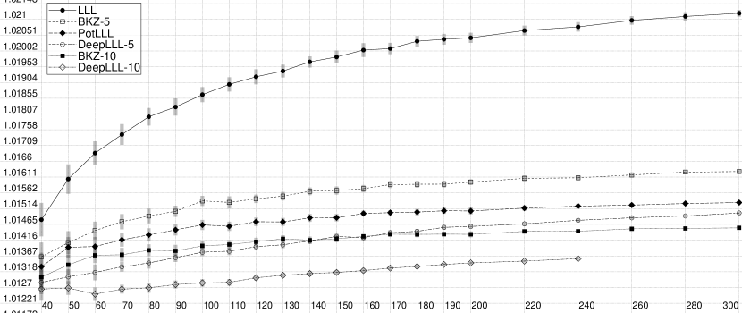
(a) Average $n$-th root Hermite factor.

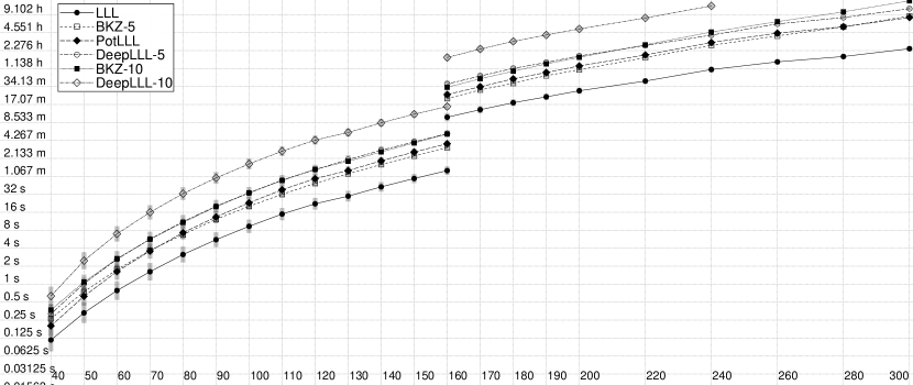
(b) Average logarithmic CPU time.

Figure 1: Overview of performance of the algorithms for dimensions $n$ ($x$ axis) from 40 to 300 (using MPFR for $n\geq 160$).

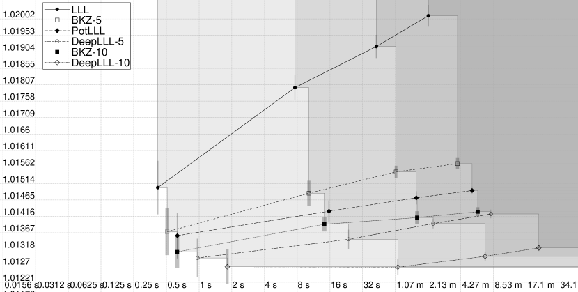
(a) long double arithmetic. The highlighted areas represent dimensions 40, 80, 120 and 160.

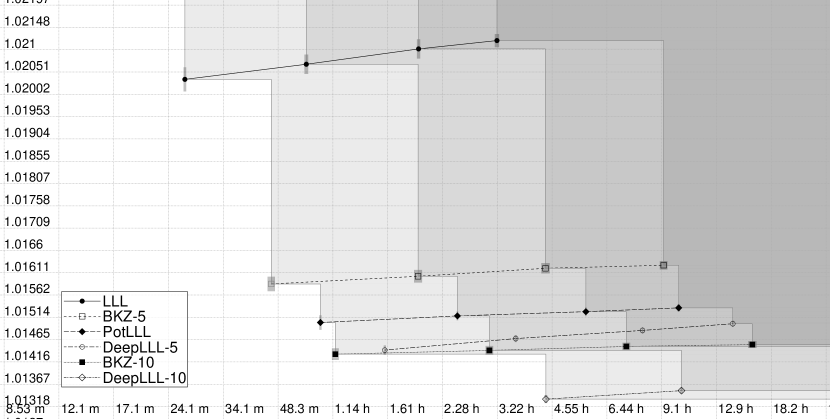
(b) MPFR arithmetic. The highlighted areas represent dimensions 180, 220, 260 and 300.

Figure 2: Comparison of $n$-th root Hermite factor ($y$ axis) vs. running times ($x$ axis) for both arithmetics for the original bases.

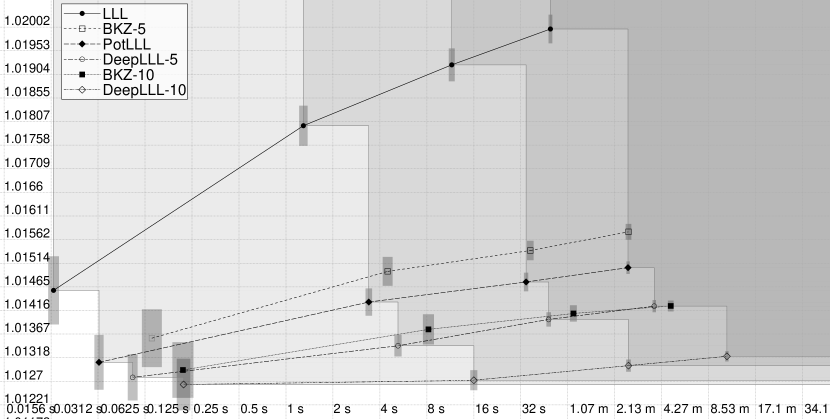
(a) long double arithmetic. The highlighted areas represent dimensions 40, 80, 120 and 160.

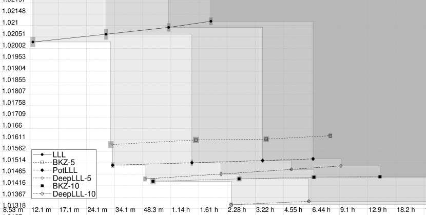
(b) MPFR arithmetic. The highlighted areas represent dimensions 180, 220, 260 and 300.

Figure 3: Comparison of $n$-th root Hermite factor ($y$ axis) vs. running times ($x$ axis) for both arithmetics for preprocessed bases (0.75-LLL-reduced bases).

5 Conclusion

We present a first provable polynomial time variant of Schnorr and Euchner’s DeepLLL. While the provable bounds are not better than for classical LLL – in fact, for reduction parameter $\delta=1$, the existence of critical bases shows that better bounds do not exist – the practical behavior is much better than for classical LLL. We see that the $n$-th root Hermite factor of an $n$-dimensional basis output by PotLLL in average does not exceed $1.0153^{n}$ for $n\leq 300$.

For unprocessed random bases in Hermite normal form, PotLLL even outperforms BKZ-5. Our experiments also show that for such bases, DeepLLL with $\beta=5$ outperforms BKZ-10. On the other hand, for bases which are already reasonably preprocessed, for example by applying 0.75-LLL to a basis in Hermite normal form, our algorithm is only slightly faster and sometimes even slower than BKZ-10, while producing longer vectors.

It is likely that the improvements of the $L^{2}$ algorithm [NS06] and the $\tilde{L^{1}}$ algorithm [NSV11] can be used to improve the runtime of our PotLLL algorithm, in order to achieve faster runtime. We leave this for future work.

Moreover, deep insertions can be used together with BKZ as well. In particular, potential minimizing deep insertions can be used. We added classical deep insertions and potential minimizing deep insertions to BKZ. First experiments up to dimension 120 suggest that with regard to the output quality, BKZ-5 with potential minimizing deep insertions is better than PotLLL, but worse than BKZ-5 with classical deep insertions, which in turn comes close to BKZ-10. BKZ-10 with potential minimizing deep insertions is close to DeepLLL with $\beta=5$, and BKZ-10 with classical deep insertions close to DeepLLL with $\beta=10$. For dimensions around 100, the speed of similarly performing algorithms also behaves similarly.

Acknowledgements

This work was supported by CASED (http://www.cased.de). Michael Schneider is supported by project BU 630/23-1 of the German Research Foundation (DFG). Urs Wagner and Felix Fontein are supported by SNF grant no. 132256.

References

- [GN08] N. Gama and P. Q. Nguyen. Predicting lattice reduction. In Advances in Cryptology—EUROCRYPT 2008, volume 4965 of LNCS, pages 31–51. Springer, 2008.
- [LLL82] A. K. Lenstra, H. W. Lenstra, Jr., and L. Lovász. Factoring polynomials with rational coefficients. Math. Ann., 261(4):515–534, 1982.
- [MG02] D. Micciancio and S. Goldwasser. Complexity of Lattice Problems: a cryptographic perspective, volume 671 of The Kluwer International Series in Engineering and Computer Science. Kluwer Academic Publishers, Boston, Massachusetts, 2002.
- [NS05] P. Q. Nguyen and D. Stehlé. Floating-point LLL revisited. In Advances in Cryptology—EUROCRYPT 2005, volume 3494 of LNCS, pages 215–233. Springer, 2005.
- [NS06] P. Q. Nguyen and D. Stehlé. LLL on the average. In F. Hess, S. Pauli, and M. E. Pohst, editors, ANTS, volume 4076 of Lecture Notes in Computer Science, pages 238–256. Springer, 2006.
- [NSV11] A. Novocin, D. Stehlé, and G. Villard. An LLL-reduction algorithm with quasi-linear time complexity: extended abstract. In STOC, pages 403–412. ACM, 2011.
- [NV10] P. Q. Nguyen and B. Vallée. The LLL Algorithm: Survey and Applications. Information Security and Cryptography. Springer Berlin Heidelberg, 2010.
- [Sch94] C.-P. Schnorr. Block reduced lattice bases and successive minima. Combinatorics, Probability & Computing, 3:507–522, 1994.
- [SE94] C.-P. Schnorr and M. Euchner. Lattice basis reduction: improved practical algorithms and solving subset sum problems. Math. Programming, 66(2, Ser. A):181–199, 1994.