Bayesian data assimilation in shape registration

Abstract

In this paper we apply a Bayesian framework to the problem of geodesic curve matching. Given a template curve, the geodesic equations provide a mapping from initial conditions for the conjugate momentum onto topologically equivalent shapes. Here, we aim to recover the well-defined posterior distribution on the initial momentum which gives rise to observed points on the target curve; this is achieved by explicitly including a reparameterisation in the formulation. Appropriate priors are chosen for the functions which together determine this field and the positions of the observation points, the initial momentum $p_{0}$ and the reparameterisation vector field $\nu$, informed by regularity results about the forward model. Having done this, we illustrate how Maximum Likelihood Estimators (MLEs) can be used to find regions of high posterior density, but also how we can apply recently developed Markov chain Monte Carlo (MCMC) methods on function spaces to characterise the whole of the posterior density. These illustrative examples also include scenarios where the posterior distribution is multimodal and irregular, leading us to the conclusion that knowledge of a state of global maximal posterior density does not always give us the whole picture, and full posterior sampling can give better quantification of likely states and the overall uncertainty inherent in the problem.

1 Introduction

Geodesics on shape space induced from diffeomorphisms are proving to be a powerful tool in the field of computational anatomy [1, 2]. Not only do they provide a notion of distance between topologically equivalent shapes, they also provide a linear characterisation of patches of shape space centred on a template image using the initial conditions of the conjugate momentum along a geodesic [3]. This permits the application of linear statistical techniques (the adaptation of principal component analysis known as principal geodesic analysis, for example [4]) since the momentum inhabits a linear cotangent space. Bayesian statistical techniques have been developed in this area in recent years, with advances in methods of determining the most likely template for a dataset as well as the most likely metric [5, 6, 7]. There are many different shape spaces: the shape of curves, landmarks, images, fibre bundles etc., but there is a unifying paradigm since in all cases the underlying velocity field that generates the diffeomorphisms that act on the shapes evolves according to the EPDiff equation [8].

In this paper, we shall address the following inverse problem: given noisy observations of points around a curve (which may have been obtained from a segmentation algorithm or human input), what is the initial momentum that generates this curve from a given template? We concentrate on the parameterisation-independent problem, in which we treat curves as being equivalent if they are related via reparameterisation. This is a challenging problem which has been addressed in a few different ways [9, 10], but here we shall make use of the approach of [11] in which a reparameterisation variable is included explicitly, and the commutation of the reparameterisation with the geodesic flow equations is exploited. In the inverse problem nomenclature, this allows us to define an observation operator that produces point values on the curve, at a cost of introducing this extra variable.

Our inverse problem can be summarised as follows. For a chosen metric, equations (5-7) together with condition (8) describe the motion along the geodesic path in the space of unparameterised curves, written in terms of a specific curve parameterisation $q(s,t)$, and a conjugate momentum $p(s,t)$, where $s$ is the parameterisation variable around the curve, and $t$ is time, i.e. the parameter along the geodesic. The initial momentum $p(s,0):=p_{0}(s)$ completely determines the direction of the geodesic, and thus the parameterisation-independent geodesic between two parameterised curves $q^{1}(s)$ and $q^{2}(s)$ can be completely described by the initial momentum $p_{0}(s)$ and a reparameterisation map $\eta(s)$ which is identified through a one-dimensional vector field $\nu(s)$. Given a template curve $q^{1}$, $p_{0}$ completely describes the final curve $q^{2}$ and $\nu$ completely describes a particular parameterisation of $q^{2}$. We wish to identify the curve $q^{2}$ which is most consistent with a set of observed data points, and we do this by defining a map $\mathcal{G}(p_{0},\nu)$ which returns a finite set of points on $q^{2}$. The inverse problem is to solve $y=\mathcal{G}(p_{0},\nu)+\eta$ given finite data $y$ and observation noise $\eta$. Since the inputs to $\mathcal{G}$ are functions and the output is a finite-dimensional vector, the problem is underdetermined.

We choose to adopt the Bayesian approach in this paper, for two main reasons. Firstly, the inverse problem of finding the geodesic flow map which deforms one shape into another from observations of the second shape is ill-posed and underdetermined. Secondly, the observations that are made are noisy in nature, and as such a probabilistic setting in which we can quantify the uncertainty inherent in the problem is appropriate. As the unknown quantities that we would like to recover are functions, we must take extra care to ensure that the problem is formulated non-parametrically[12]. As such, we look to follow the methodologies that have been utilised previously in various fluid mechanics problems [13, 14, 15].

Once the Bayesian inverse problem has been defined in such a way as to be well-posed on function space, we must consider how appropriate algorithms can be implemented on a computer in order to characterise the posterior probability distributions on the unknown functions. The unknown functions are of course discretised within the algorithms, and because it may be desirable to refine the mesh to obtain further accuracy, it is important that the MCMC methods used to sample the posterior converge in distribution at rates independent of the discretisation used. A range of MCMC methods which are well-defined on function space (and as such have mixing rates which are independent of discretisation of those functions) are available[16], and have been used for Bayesian inverse problems on function spaces[14, 15]. The properties of these algorithms make them a highly viable candidate for the analysis of the problems identified in this paper. Specifically, a function space analogue of the random walk Metropolis-Hastings (RWMH) algorithm will be used in the numerical examples in this paper, referred to in [12, 16] as the pCN algorithm.

In Section 2 we introduce the problem, and describe the equations of motion of the shape as it is deformed by the velocity field, and demonstrate how we can find geodesic paths in shape space between two shapes. We also show in this section that the deformed shape is Lipschitz continuous with respect to two functions, the initial momentum $p_{0}$, and the reparameterisation function $\nu$. In order to tackle an inverse problem on function spaces, it is necessary to show that this problem is well-posed. This amounts to finding function spaces on which the forward problem is locally Lipschitz, and in Section 3 we find sufficient conditions on the regularity of these spaces. In Section 4 we frame the inverse problem as a well-posed Bayesian inverse problem, and identify minimum regularity priors for the functions, informed by the analysis in Section 3.

In Section 5 we describe the Markov chain Monte Carlo (MCMC) algorithm that we use to sample directly from the well-defined posterior density on $p_{0}$ and $\nu$. In Section 6 we briefly discuss how we numerically approximate the dynamics described in Section 2, before presenting some illustrative numerical examples in Section 7. We finish in Section 8 with some conclusions and discussion.

2 Description of the forward model

In this section, we review the equations of motion for curves in the plane acted on by geodesics in the diffeomorphism group, and explain how these equations can be used to provide a mapping from the space of periodic scalar functions (which turn out to be the normal component of a conjugate momentum variable) to topology-preserving nonlinear deformations of some chosen curve in the plane. We then provide some analytical results that are required for defining the associated Bayesian inverse problem.

In our approach, we parameterise an oriented curve in the plane as a continuous function $q$ from a space $S$ (such as the circle, $S^{1}$) into $\mathbb{R}^{2}$ i.e., $q\in C^{0}(S^{1},\mathbb{R}^{2})$. Although in this paper we concentrate on the lower dimensional case of a curve in the plane, it may be extended to surfaces in $\mathbb{R}^{3}$, which provides many applications in medical imaging, for example. We parameterise an evolving curve as $q(s,t)$, where $s\in S$ is the parameter around the curve, and $t\in[0,1]$ is the time parameter. Following the methodology of [17, 18, 10] we constrain the motion of the curve $q(s,t)$ to the action of diffeomorphisms by requiring that

$$\frac{\partial}{\partial t}q(s,t)=u(q(s,t),t)$$ (1)

where $u(x,t)$ is a time-parameterised family of vector fields on $\mathbb{R}^{2}$. This guarantees that the topology of the curve is preserved (i.e. there are no overlaps or cavitations). We wish to study curve evolution from a template curve $\Gamma^{1}$ (parameterised by $q^{1}(s)$) to a target curve $\Gamma^{2}$ (parameterised by $q^{2}(s)$). However, since we only want information about the shape of the curve, and not the specific parameterisation, we do not wish to enforce that any specific point $q^{1}(s)$ gets mapped to any specific point on $\Gamma^{2}$. We instead use the following generalised boundary condition

$$q(s,0)=q^{1}(\eta(s)),\quad q(s,1)=q^{2}(s),$$ (2)

for arbitrary reparameterisations $\eta\in\operatorname{Diff}_{+}(S)$, the orientation-preserving subgroup of the diffeomorphism group $\operatorname{Diff}(S)$ on $S$. If the boundary conditions (2) are satisfied, we say that $u$ describes a path between $\Gamma^{1}$ and $\Gamma^{2}$. We select a function space $B$ for vector fields, and define the distance along the path as

$$\int_{0}^{1}\frac{1}{2}\|u\|^{2}_{B}\operatorname{d\!}{t}.$$ (3)

For simplicity we assume that $B$ is a Hilbert space and that there exists an operator $A$ such that

$$\|u\|^{2}_{B}=\langle u,Au\rangle_{L^{2}}.$$ (4)

The shortest path between $\Gamma^{1}$ and $\Gamma^{2}$ is defined by minimising (3) over $u$ and $\eta$ subject to (1) and the boundary conditions (2). To obtain the equations of motion for the shortest path, we introduce Lagrange multipliers $p(s,t)$ (which we call the “momentum”) to enforce (1), and seek extrema of the action

$$\mathcal{A}=\int_{0}^{1}\frac{1}{2}\|u\|^{2}_{B}+\langle p,\dot{q}-u(q)\rangle\operatorname{d\!}{t}.$$

This leads to the following equations of motion in weak form:

$$\langle\delta u,Au\rangle_{L^{2}}-\langle p,\delta u(q)\rangle = 0,$$ (5)

$$\int_{0}^{1}\left\langle\delta p,\frac{\partial q}{\partial t}-u(q)\right\rangle\operatorname{d\!}{t} = 0,$$ (6)

$$\int_{0}^{1}\left\langle p,\frac{\partial\delta q}{\partial t}-(\nabla u(q))\delta q\right\rangle\operatorname{d\!}{t} = 0,$$ (7)

where $\delta p$ and $\delta q$ are space-time test functions, with

$$u,\delta u\in B,\quad p,\delta p\in L^{2},\quad q,\delta q\in H^{1}.$$

If the minimisation is taken over all reparameterisations $\eta\in\operatorname{Diff}_{+}(S)$ then we obtain the condition

$$p\cdot\frac{\partial q}{\partial s}=0,\quad\forall t\in[0,1].$$ (8)

The condition states that the momentum $p$ is normal to the shape. As described in [11], if this condition is satisfied, then the curve evolution is invariant under the transformation

$$(p,q)\mapsto(\bar{p},\bar{q})=\left({p\circ\eta}{\frac{\partial\eta}{\partial s}},q\circ\eta\right)$$ (9)

for $\eta\in\operatorname{Diff}_{+}(S)$, which is the cotangent-lift of the transformation $q\mapsto q\circ\eta$. This means that if equations (5-7) are solved with initial conditions $(p,q)$ and $(\bar{p},\bar{q})$ then $\bar{q}=q\circ\eta$ at time 1. As described in [19], solutions that satisfy equation 8 are parameterised realisations of geodesics on the shape space $C^{0}(S^{1},\mathbb{R}^{2})/\operatorname{Diff}_{+}(S)$.

We define the time-1 flow map $\Psi$

$$\Psi(p|_{t=0},q|_{t=0})=q|_{t=1},$$

where $p$ and $q$ satisfy equations (5-7). Having fixed $q|_{t=0}=q^{1}$, we define a parameterisation-independent mapping between scalar functions $p_{0}:S\mapsto\mathbb{R}$ (the normal component of the initial conditions of $p$) and topologically equivalent curves $q^{2}$ obtained by

$$q^{2}=\Psi(p_{0}n,q^{1}),$$

where $n$ is the normal vector to the curve $q^{1}$. The power of this mapping is that it allows us to perform linear operations on the space of functions $p_{0}$, such as averages.

In this paper, our aim is to estimate the probability measure for $p_{0}$ given a set of observed points $(q_{1},\ldots,q_{n})$ from the curve $q^{2}$. These points may have been obtained from a digitised medical image, for example. These points are assumed to be sorted in order according to the orientation of the curve. We cannot directly solve the inverse problem of finding $p_{0}$ such that

$$\Psi(p_{0}n,q^{1})(s_{i})=q_{i},\qquad i=1,\ldots,n,$$

since we do not know the values $s_{i}$ of the curve parameter $s$ that correspond to each $q_{i}$. To fix this, we introduce a reparameterisation variable $\eta\in\operatorname{Diff}_{+}(S^{1})$, and seek $(p_{0},\eta)$ such that

$$\Psi\left(\left(p_{0}n\right)\circ\eta\,\frac{\partial\eta}{\partial s},q^{1}\circ\eta\right)(s_{i})=q_{i},\quad i=1,\ldots,n,$$

with $\{s_{i}\}_{i=1}^{n}$ is some chosen distinct sequence of points in $S$ ordering according to orientation, e.g. equispaced points. This guarantees to preserve the ordering since the curve is evolved by a diffeomorphism. The introduction of the reparameterisation variable does not alter the shape of the obtained curve, just the particular parameterisation used.

Following [20], we construct reparameterisations from scalar periodic functions $\nu$ by solving

$$\frac{\partial\chi}{\partial t}(s,t)=\nu(\chi(s,t)),\quad\chi(s,0)=\operatorname{Id},\quad\chi(0,t)=\chi(1,t),0\leq t,$$ (10)

where $\operatorname{Id}$ is the identity map ($\operatorname{Id}(s)=s$). The reparameterisation map is then evaluated from $\eta(s)=\chi(s,1)$. The function $\nu$ represents the generating vector field for the reparameterisation $\eta$ on the scalar interval $[0,1]$ with periodic boundary conditions. This is known as Lie exponentiation, and guarantees that $\eta$ is an orientation preserving, smooth invertible map (for sufficiently smooth $\nu$). This defines a reparameterisation map:

$$\mathcal{R}(p,q,\nu)=\left({\left(p_{0}n\right)\circ\eta}{\frac{\partial\eta}{\partial s}},q^{1}\circ\eta\right)$$

where $\eta$ is obtained from (10). An illustrative diagram is given in Figure 1.

Figure 1: Diagram illustrating the forward model. Curves are shown with highlighted points to indicate the parameterisation. The reparameterisation velocity $\nu$ generates a reparameterisation of the curve (which also transforms the initial momentum $p_{0}$), and then the (transformed) initial momentum $p_{0}$ generates an evolution of the curve by the time-1 flow map of equations (5-7). For the undiscretised equations changing $\nu$ but not $p_{0}$ leads to different parameterisations of the same curve, since reparameterisation and the time-1 flow map commute.

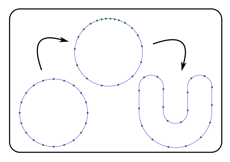
Hence we define the observation operator $\mathcal{G}$ by

$$\mathcal{G}(p_{0},\nu)=\left(\begin{array}[]{c c}G(s_{i})\\ \vdots\\ G(s_{n})\\ \end{array}\right),$$ (11)

where $G=\Psi\circ\mathcal{R}(p_{0}n,q^{1},\nu)$. The normal component of $p_{0}$ then characterises the shape of the target curve $\Gamma^{2}$ relative to the curve $\Gamma^{1}$, whilst the generator variable $\nu$ merely describes the reparameterisation of the target curve which is obtained at the minimum.

3 Properties of the Observation Operator

In this section, we show that the observation operator $\mathcal{G}$, given in Equation (11), is Lipschitz in $p_{0}$ and $\nu$, for appropriately chosen spaces. We make the following definition.

Definition 1.

We say that a Hilbert space $B$ of vector fields is embedded in $C^{n}(\Omega,\mathbb{R}^{d})$ if there exists a constant $C_{e}$ s.t. $\|v\|_{n,\infty}\leq C_{e}\|v\|_{B}$. In that case we also say for notational convenience that $B$ is $[-$admissiblen].

We adopt the notation that $\nu\in D$. The main result of this section is the following Theorem.

Theorem 2.

1. Let $B$ be $[-$admissible2], and $D$ be $[-$admissible1]. Then for $q_{0}\in W^{1,\infty}$, the observation operator $\mathcal{G}$ is a Lipschitz continuous map from $(L^{2},D)$ to $\mathbb{R}^{2n}$.

2. Let $B$ be $[-$admissible3] and $D$ be $[-$admissible1]. Then for $p_{0}\in H^{-1}$ and $q_{0}\in W^{1,\infty}$, the observation operator $\mathcal{G}$ is Lipschitz continuous.

To show that $\mathcal{G}$ is Lipschitz, we first prove existence, uniqueness and Lipschitz continuity for the maps $\Psi$ and $\mathcal{R}$. This is then used to show that the observation operator is Lipschitz continuous with respect to the normal component $p_{0}$ of the initial conditions $p$ and the generator variable $\nu$.

Let $B$ be the space of vector fields, $Q$ be a Hilbert space and $P$ be its dual. Here $Q$ represents a space of curves with a particular norm, for example $Q=L^{2}(S_{1},\mathbb{R})$ or $Q=H^{1}(S_{1},R)$. We want to define the momentum map as given by

$$J:(p,q)\in P\times Q\mapsto J(p,q):=\left(v\mapsto\left\langle p,v\circ q\right\rangle_{P,Q}\right)\in B^{*}\,.$$ (12)

Here $B^{*}$ represents the dual space of $B$, the space of linear operators acting on $B$. In this aim, we assume in addition that the map $B\times Q\mapsto Q$ defined by $(v,q)\to v\circ q$ is a Lipschitz map on $Q$ for a fixed $v\in B$ namely there exists $C_{c}$ s.t.

$$\|v\circ q_{1}-v\circ q_{2}\|_{Q}\leq C_{c}\|v\|_{B}\|q_{1}-q_{2}\|_{Q}\,.$$ (13)

As a consequence, since this composition map is linear on $B$, the map is Lipschitz on $B\times Q$. This assumption makes $J(p,q)$ well-defined and Lipschitz on $P\times Q$ for the dual norm on $B^{*}$.

Lemma 3.

The assumption above is satisfied in the following situations

• $B$ is $[-$admissible1] and $P=Q=L^{2}(S_{1},\mathbb{R})$.

• $B$ is $[-$admissible2], $P=H^{-1}(S_{1},\mathbb{R})$ and $Q=H^{1}(S_{1},\mathbb{R})$.

Proof.

For both points, we use the integration formula for the path $q(t)=tq_{1}-(1-t)q_{0}$

$$f(q(1))-f(q(0))=\int_{0}^{1}df(q(t))(q_{1}-q_{0})\,dt\,,$$ (14)

for $f\in C^{1}$. For the first point, for any $f\in C^{1,\infty}(\mathbb{R}^{d},\mathbb{R}^{d})$,

$$\|f\circ q_{1}-f\circ q_{2}\|_{L^{2}}\leq\|f\|_{1,\infty}\|q_{1}-q_{2}\|_{L^{2}}\,,$$ (15)

which gives the result. For the second point, we note that $H^{1}(S_{1},\mathbb{R})$ is Banach algebra, namely for any couple $(f,g)\in H^{1}(S_{1},\mathbb{R})$ we have

$$\|fg\|_{H^{1}}\leq\|f\|_{\infty}\|g\|_{H^{1}}+\|g\|_{\infty}\|f\|_{H^{1}}\leq 4\|f\|_{H^{1}}\|g\|_{H^{1}}\,.$$

Therefore in the Formula (14), the term $df(q(t))(q_{1}-q_{0})$ can be understood as the product (generalised to $\mathbb{R}^{d}$) of two elements in $H^{1}(S_{1},\mathbb{R}^{d})$ provided that $df(q(t))$ belongs to $H^{1}$. Moreover $H^{1}$ is stable under the composition with a $C^{1}$ function bounded for

$$\|f\circ q\|_{H^{1}}=\|f\|_{1,\infty}\|q\|_{H^{1}}$$ (16)

The second point then follows from

$$\|f\circ q_{1}-f\circ q_{2}\|_{H^{1}}\leq\|f\|_{2,\infty}\|q_{1}-q_{2}\|_{H^{1}}\,,$$ (17)

∎

We write Equations (5-7) as follows:

$$\dot{q} = u\circ q$$ (18)

$$\dot{p} = -\nabla u(q).p$$ (19)

$$u = J(p,q)^{\sharp}\,,$$ (20)

where $J(p,q)^{\sharp}$ denotes the corresponding element in $B$ given by the Riesz theorem, i.e.

$$\langle J(p,q)^{\sharp},v\rangle_{B}=J(p,q)(v)\,.$$

Equation (19) is a pointwise matrix multiplication when $p$ is smooth. When $p\in H^{-1}$ for instance, the operation is defined by duality, defined as follows.

Definition 4.

Let $Q$ be a Banach algebra then the multiplication $Q^{*}\times Q\mapsto Q$ is defined by duality

$$\langle q_{1}.\,p,q_{2}\rangle=\langle p,q_{1}q_{2}\rangle$$ (21)

Remark 5.

The multiplication on a Banach algebra is by definition bilinear continuous. As a consequence, the multiplication inherits the same properties and in particular, the Lipschitz property.

We now prove that these shooting equations are a simple ODE in infinite dimensions i.e. $\dot{X}=F(X)$ with state variable $X$ in a Banach space; This function $F$ satisfies the classical Lipschitz assumption which means that solutions can be obtained using Picard’s fixed point method; it also ensures that the solutions are Lipschitz functions of the initial conditions.

Lemma 6.

System (18-20) is an ODE on $P\times Q$ which satisfies the Lipschitz condition for the two following cases on bounded balls in $P\times Q$:

• $B$ is $[-$admissible2], $P=L^{2}$ and $Q=L^{\infty}$

• $B$ is $[-$admissible3], $P=H^{-1}$ and $Q=H^{1}$ .

Remark 7.

The space $Q=L^{\infty}(S_{1})$ is not a Hilbert space in this case but only a Banach space.

Proof.

In the two claimed cases, we have by Proposition 3 that $(p,q)\to J(p,q)^{\sharp}$ is Lipschitz for the norm on $B$. Then using the inequality (15), we deduce that $(p,q)\to J(p,q)^{\sharp}\circ q$ is Lipschitz as the composition of two Lipschitz functions. Thus, we have treated the first component (18) of the ODE.

Using Remark 5, it is then sufficient to prove that $(p,q)\in P\times Q\mapsto d[J(p,q)^{\sharp}](q)\in Q$ is a Lipschitz mapping. Denoting $v_{i}=J(p_{i},q_{i})^{\sharp}$ for $i=1,2$, use of the triangle inequality gives

$$\|dv_{1}\circ q_{1}-dv_{2}\circ q_{2}\|_{Q} \leq C_{e}\|v_{1}\|_{B}\|q_{1}-q_{2}\|_{Q}+\|dv_{1}\circ q_{2}-dv_{2}\circ q_{2}\|_{Q}$$ (22)

$$\leq C_{e}\|v_{1}\|_{B}\|q_{1}-q_{2}\|_{Q}+C_{e}\|v_{1}-v_{2}\|_{B}\|q_{2}\|_{q}\,,$$

where we rely on the inequality (17) for the $H^{1}$ case and (15) for the first case.

Up to this point, we only have proven a local Lipschitz condition. It remains to prove that for $(p_{0},q_{0})\in B(0,r)\subset P\times Q$ with $r$ a positive real number, there exists a constant $M_{r,t}$ (the subindex indicating that this constant only depends on $r$ and the time $t$) such that for all time $t\geq 0$ the system (18-20) is Lipschitz of Lipschitz constant $M_{r}$. In particular this implies that the solutions are defined for all times. To this end, we remark that the geodesic equations (18-20) are variational with the Hamiltonian is constant in time. This can be checked by a straightforward calculation. Since the Hamiltonian reads $H(p,q)=\left\|J(p,q)^{\sharp}\right\|_{B}^{2}$, the Lipschitz inequality (22) becomes

$$\|dv_{1}\circ q_{1}-dv_{2}\circ q_{2}\|_{Q}\leq 3r\,C_{e}\,\|q_{1}-q_{2}\|_{Q}\,.$$ (23)

For the equation (18), the inequality (13) implies

$$\left\|v_{1}\circ q_{1}-v_{2}\circ q_{2}\right\|\leq rC_{c}\left\|q_{1}-q_{2}\right\|_{Q}+\left\|v_{1}-v_{2}\right\|_{B}\max{(\left\|q_{1}\right\|_{Q},\left\|q_{2}\right\|_{Q})}$$ (24)

but by direct integration of Inequality (13) we see that $\max{(\left\|q_{1}\right\|_{Q},\left\|q_{2}\right\|_{Q})}\leq C_{c}\,r\,t$ for any time $t>0$. A similar inequality holds for the momentum $p$, hence the geodesic equations (18-20) are Lipschitz for a constant $M_{r,t}$ that has polynomial growth in $t$ and in $r$. ∎

We now claim the following result which is based on Grönwall’s lemma.

Lemma 8.

Solutions of the geodesic equations (18-20) have a Lipschitz dependency w.r.t. their initial conditions for their respective norms.

We are now in a position to prove Theorem 2.

Proof.

The observation operator $\mathcal{G}$ is the evaluation at points $(\eta(s_{i}))_{i=1}^{n}$ of the deformed template $q(1)$ obtained by the geodesic equations (18-20) without reparameterisation. In other words,

$$\textrm{Ev}(p_{0},q_{0},\nu)=\left(\begin{array}[]{c}q(1)\circ\eta(s_{1})\\ \vdots\\ q(1)\circ\eta(s_{n})\\ \end{array}\right)$$ (25)

where $q(1)$ is the solution at time $1$ of the geodesic equations (18-20) for initial data $p_{0},q_{0}$ and $\eta$ is the Lie exponential of $\nu$. To prove that the observation operator is Lipschitz in those three variables, we observe that it is the composition of the flow of the geodesic equations (18-20) and the right composition with the reparameterisation by $\eta$. The first operation is Lipschitz continuous by Corollary (8). Now the right composition is also Lipschitz continuous since $q(1)\in W^{1,\infty}$ (indeed since $B$ is $[-$admissible2] or $[-$admissible3], the flow of the geodesic equations (18-20) preserves $W^{1,\infty}$) we have

$$\|q(1)\circ\eta_{1}-q(1)\circ\eta_{2}\|_{\infty}\leq\|\nabla q(1)\|_{\infty}\|\eta_{1}-\eta_{2}\|_{\infty}\leq M\|\nabla q(1)\|_{\infty}\|\nu_{1}-\nu_{2}\|_{D}\,.$$ (26)

∎

4 Bayesian Inversion

In this section, we aim to frame the ill-posed inverse problem of finding $(p_{0},\nu)$ given noisy observations of the target shape, as a well-posed Bayesian inverse problem on function space. The “solution” to this inverse problem is then given by a probability distribution. Bayes’ formula allows us to construct, through combining prior beliefs about the functions, with observations of the system, the posterior distribution of the possible values that the unknown functions could have taken.

4.1 Prior Distributions

Extra care must be taken in this context, since the unknowns are functions, and as such the problem must be formulated non-parametrically. Following the philosophy of [12], we use the results from Section 3 to identify minimum regularity priors which will ensure that the problem is well-defined. For problems on infinite dimensional spaces, we must identify prior distributions for the functions, which have full measure with respect to function spaces on which the observation operator is Lipschitz continuous. Theorem 9 summarises these results for the problem presented in this paper, and follows at the end of this section.

The role of the prior in this respect is two-fold. The prior can contain prior information or beliefs about the form or structure of the solution, possibly taken from previous observations. However another important role of the prior is to regularise the problem, to make it well-posed. Indeed it plays a very similar role to the penalty term in a Tikhonov regularisation, an optimisation formulation of the inverse problem. We will explore these similarities in Section 5.1, and exploit them in our numerical method.

4.2 Observations and the Likelihood

Uncertainty in this problem arises from errors incurred during observation. Observational noise is often modelled as being additive Gaussian. This uncertainty in the exact shape of the curve leads to uncertainty in the value of the pair of functions which would deform the reference shape to the observed shape. Understanding and quantifying that uncertainty is a key part of solving this problem, as naive least squares matching to the data would lead to an ill-posed problem.

We assume that observations $y$ of the quantity of interest are noisy in nature, satisfying:

$$y=\mathcal{G}(p_{0},\nu)+\xi,\qquad\xi\sim\mathcal{N}(0,\Sigma),$$

where $\Sigma$ is assumed to be known, and where $\mathcal{G}$ is defined to be the observation operator given by (11). That is, the function which returns to us what noiseless observations we would make if we were to deform the template shape and reparameterise using the function pair $(p_{0},\nu)$. This assumption allows us to compute the likelihood that $y$ was observed with a given $(p_{0},\nu)$, through the probability density function of $\xi$:

$$\mathbb{P}(y|p_{0},\nu)\propto\operatorname{exp}\left(-\frac{1}{2}\|\mathcal{G}(p_{0},\nu)-y\|^{2}_{\Sigma}\right),$$ (27)

where $\|x\|^{2}_{\Sigma}:=x^{T}\Sigma^{-1}x$ is the covariance weighted norm.

4.3 Bayes’ Theorem and the Posterior

Bayesian inversion is one way to regularise an ill-posed inverse problem, and convert this into a well-posed one. Bayes’ formula is central to this. Prior beliefs about the quantities of interest are blended with data from observations to give the posterior $\mathbb{P}(u|y)$ distribution. The finite dimensional version of this formula is

$$\mathbb{P}(u|y)\propto\mathbb{P}(y|u)\mathbb{P}(u),$$

where $u$ denotes the unknown quantity that we wish to characterise from the data, $\mathbb{P}(u)$ the probability distribution describing our prior beliefs about those quantities, and $\mathbb{P}(y|u)$ the likelihood function, which returns the likelihood that we would make the observations $y$ given a particular value of the quantity $u$.

However, in this paper the quantity of interest is a pair of functions $u=(p_{0},\nu)$. In this infinite dimensional setting, we must use the analogous result regarding the Radon-Nikodym derivative of the posterior distribution with measure $\mu$, with respect to the prior distribution on $(p_{0},\nu)$ with measure $\mu_{0}$:

$$\frac{d\mu(p_{0},\nu)}{d\mu_{0}}\propto\mathbb{P}(y|(p_{0},\nu)),$$ (28)

where the likelihood expression is given by (27).

Note that this formula only holds if the posterior is indeed absolutely continuous with respect to the prior distribution, otherwise no such derivative is admitted. Sufficient conditions on the priors for this to be satisfied are given in the following section.

4.4 Prior and Posterior Distributions on $(p_{0},\nu)$

Before stating the main result of this Section, we must first introduce some notation. Let us consider the Helmholtz operator with periodic boundary conditions

$$\mathcal{H}=I-\ell^{2}\frac{\partial^{2}}{\partial s^{2}},$$

where $\ell\in\mathbb{R}$ defines a characteristic length scale. Note also that for samples $u\sim\mathcal{N}(0,\delta\mathcal{H}^{-\alpha})$ for some $\alpha>\beta+\frac{d}{2}$ for some $\beta\geq 0$, then $u\in H^{\beta}$ almost surely (follows from [12]). The length scale parameter $\ell\in\mathbb{R}^{+}$ allows us to control at which scale the smoothing properties of the Laplacian take effect. With a larger value of $\ell$, a larger value of $|k|$ is required before the effect of the Laplacian becomes dominant. Likewise, as $\ell\to 0$, $\mathcal{H}\to-\Delta$, meaning that the Laplacian is dominant on all scales. The choice of this value, however, does not affect the overall regularity of samples drawn from the distribution $\mathcal{N}(0,\mathcal{H}^{-\alpha})$.

Theorem 9.

Let $B$ be 3-admissable, $D$ be 1-admissable, and $\mu_{0}(p_{0},\nu)=\mathcal{N}(0,\delta_{1}\mathcal{H}_{1}^{-\alpha_{1}})\times\mathcal{N}(0,\delta_{2}\mathcal{H}_{2}^{-\alpha_{2}})$ for $\alpha_{1}>-\frac{1}{2}$, $\alpha_{2}>3/2$, $\delta_{1},\delta_{2}\neq 0$, and where $\mathcal{H}_{i}=(\ell_{i}I-\Delta)$ where $\ell_{i}\in\mathbb{R}^{+}$ for $i\in\{1,2\}$. Then $\mathcal{G}$ is measurable with respect to $\mu_{0}$, and the posterior measure $\mu$ is absolutely continuous with respect to $\mu_{0}$, with Radon-Nikodym derivative given by (28).

Proof.

Result follows by the Sobolev embedding theorem, results in [12], and Theorem 2. ∎

For the posterior distribution to be well-defined, it must be absolutely continuous with respect to the choice of prior distribution on the two unknown functions of interest. This choice of prior distribution is informed by the properties of the forward model, and the observation operator $\mathcal{G}$. Theorem 9 gives us Gaussian priors which have sufficient regularity to ensure that this condition is met.

5 Characterising the Posterior Density

In this section we introduce the statistical methods which we use in order to characterise the posterior distribution of the function pair $(p_{0},\nu)$ given a choice of prior distribution and a set of noisy observations of the target shape. Monte Carlo Markov chains (MCMC) are a set of tools which allow us to sample from a desired probability distribution. A chain of states is formed, which converges in distribution to the target density. We then describe a method for initialising the MCMC method efficiently.

5.1 The Function Space Random Walk Metropolis-Hastings algorithm (pCN)

For the purpose of the numerics, we use a version of the Random Walk Metropolis Hastings (RWMH) algorithm framed on function spaces, referred to as the pCN algorithm[12, 16]. This method is superior to the usual vanilla random walk method in that it is well-defined on function spaces, and as such is robust under refinement of any discretisation of the forward model [16]. This means that the rate of convergence of statistics in the Markov chains are independent of this discretisation, whereas the Metropolis Hasting algorithm with vanilla random walk proposal degenerates as the forward model’s discretisation is refined. The following describes the pCN sampler, where $\Phi=\frac{1}{2}\|\mathcal{G}(p_{0},\nu)-y\|^{2}_{\Sigma}$:

1:  $u_{0}=(p_{0},\nu)_{0}$

2:  for $i=1:N$ do

3:     Sample $v=(1-\beta^{2})^{1/2}u_{i-1}+\beta w$, where $w\sim\mu_{0}((p_{0},\nu))$

4:     $a(u_{i-1},v)=\min\left\{1,\operatorname{exp}(\Phi(u_{i-1})-\Phi(v)\right\}$

5:     Sample $u\sim U([0,1])$

6:     if $u<a(u_{i-1},v)$ then

7:        $u_{i}=v$

8:     else

9:        $u_{i}=u_{i-1}$

10:     end if

11:  end for

The acceptance probability in this algorithm is independent of the approximation method used for the unknown functions, and as such has superior mixing properties as compared with standard methods for finer discretisations. Further to this basic algorithm, we can alter this to also use the data to infer on the variance of the observational noise, if we no longer assume that this is known[16]; we make use of this in the numerical experiments in Sections 7.1 and 7.3.

MCMC methods usually need a period of “burn-in” in which we try to ensure that the chain starts in a region which is not in the tails of the posterior distribution. MAP estimators can be used to try to find regions of high posterior density, as described in [13]. For the problem as we have defined it, this equates to finding the solution to:

$$\min_{p_{0}\in L^{2},\nu\in H^{2}}L(p_{0},\nu)=\min_{p_{0}\in L^{2},\nu\in H^{2}}\frac{1}{2}\|\mathcal{G}(p_{0},\nu)-y\|^{2}_{\Sigma}+\frac{1}{2}\|(p_{0},\nu)\|^{2}_{\mu_{0}}$$

where $\|(\cdot,\cdot)\|_{\mu_{0}}$ is the equivalent penalty term to that induced in the posterior measure by the choice of prior measure $\mu_{0}$, or the Cameron-Martin norm corresponding to $\mu_{0}$. In particular, if (as is the case for our purposes) $\mu_{0}(p_{0},\nu)=\mathcal{N}(0,\delta_{1}\mathcal{H}^{-\alpha_{1}})\times\mathcal{N}(0,\delta_{2}\mathcal{H}^{-\alpha_{2}})$, then

$$\|(p_{0},\nu)\|^{2}_{\mu_{0}} = \sum_{k}\delta_{1}|p_{k}|^{2}(\ell_{1}-|k|^{2})^{\alpha_{1}}+\delta_{2}|\nu_{k}|^{2}(\ell_{2}-|k|^{2})^{\alpha_{2}}$$

Various descent methods can be used to try to find local minima of this quantity. Most of these methods incorporate gradient information of some type to attempt to search for the minima in appropriate directions. These methods include steepest descent and conjugate gradient among others.

The method that we will utilise in our numerics in order to initialise our Markov chains is called the Broyden-Fletcher-Goldfarb-Shanno (BFGS) method [22, 23]. This method uses the gradient information from the last two states in the chain to approximate a Hessian matrix, which is then used to choose an appropriate direction in which to search for the local minimum.

Once the BFGS method has converged within certain tolerances, the state that has been settled on can be used as an initial state in the MCMC chain. Assuming that the BFGS method has converged close to a global or even local maxima of probability density, then the chain will more quickly enter probabilistic equilibrium. For example, consider the data used in Section 7.3. The ratio of probability densities of the state $(p_{0},\nu)=(0,0)$ with the state the BFGS method converged to was $\operatorname{exp}(-958.85)$, a huge difference.

6 Numerical Approximation of $\mathcal{G}$

The observation operator consists of the concatenation of four maps: 1) the generation of the reparameterisation variable $\eta$ from the vector field $\nu$ according to (10), 2) the application of the reparameterisation formula according to (9), 3) the time-1 flow map of the geodesic equations according to (5-7), and 4) the evaluation of the curve $q|_{t=1}$ at the finitely chosen points. Stages (1) and (3) are both numerically discretised using particle-mesh methods as described in [24]. These methods allow efficient evaluation of the velocity field at particle locations whilst preserving variational structure and making it possible to compute the exact adjoint equations of the discrete system which are used in the implementation of the deterministic burn-in. Stages (2) and (4) use cubic B-spline interpolation, which also make computing the adjoint tractable. Details of the numerical approximation procedure, along with numerical tests that show that the numerical scheme is second-order convergent in space, are given in [20]. In summary, the discretisation replaces the parameterised curve $q(s)$ as an ordered discrete set of points $\{q_{i}\}_{i=1}^{n_{p}}$, similarly the conjugate momentum $p(s)$ is replaced by a set ${p_{i}}_{i=1}^{n_{p}}$ of (co)-vectors associated with each point. Convergence is achieved as $n_{p}\to\infty$, assuming a sufficiently smooth velocity field; the convergence rate was demonstrated to be second-order in [20]. The velocity field $u$ is discretised on a static, uniform mesh with $n_{g}\times n_{g}$ grid points. In the numerical algorithm, the momentum is interpolated from the points to the grid using cubic B-splines; the elliptic operator A is then approximately inverted on the grid using discrete Fourier transform, and the resulting velocity is interpolated back to the points $q_{i}$. As described in [24], this interpolation preserves the Hamiltonian structure of the equations, and as described in [20], allows an exact adjoint of the numerical model to be constructed, which is used to obtain derivatives of the observation operator. Convergence was also demonstrated to be second-order as $n_{g}\to\infty$ in [20]. Alternatively, one can select a finite value for $n_{g}$ whilst keeping $q$ and $p$ continuous; this just leads to a modification of the operator $A$. The discretisation for the reparameterisation variable $\nu$ was introduced in [20]. The reparameterisation velocity $\nu(s)$ is also discretised as a discrete set of values $\{\nu_{i}\}_{i=1}^{n_{p}}$, and the reparameterisation map is obtained by interpolating $\nu$ to the reparameterised locations; $q$ and $p$ are then pulled back under the reparameterisation map by interpolation. As discussed in [11], reparameterisation and flow along geodesics are commuting operations; in [20] the commutation error was shown to converge to zero at second-order as $n_{p}\to\infty$.

7 Numerical Results

We present numerical results to show that the algorithm is successfully drawing samples from the posterior distribution, and then go on to study the posterior distribution in certain data scenarios. The first thing to address is our choice of template shape $\Gamma^{1}$ and the parameterisation $q^{1}(s)$ that we use for this shape. Since we are only considering closed curves, it seems natural to choose a circle for this to keep things as simple as possible. We also wish to choose a nice smooth parameterisation for this shape, centred in the middle of our domain $\mathbb{T}^{2}=[0,2\pi)^{2}$ so we pick

$$q^{1}(s)=(\cos(s)+\pi,\sin(s)+\pi),\qquad s\in[0,2\pi).$$ (29)

We will engage in simulation studies in which the data is itself produced by employing the numerical simulation of a forward PDE model. In all the numerics, we assume that the noise $\xi$ through which we make the observations

$$y=\mathcal{G}(p_{0},\nu)+\xi,\qquad\xi\sim\mathcal{N}(0,\Sigma),$$

has a diagonal covariance matrix $\Sigma$, which we describe for each experiment.

In terms of the approximation of the forward model in the algorithm, 50 time steps are used in which to deform the parameterisation of the shape from time $t=0$ to $t=1$. The curves themselves are approximated by 100 points, and with a $64\times 64$ grid approximating the underlying velocity field. The values of $s_{j}$ at which observations are made are given by $\left\{\frac{2\pi s_{j}}{N}\right\}_{j=0}^{N-1}$. These parameters are used in the model to create the data, and in the implementation of the statistical algorithm.

The prior distributions on $p_{0}$ and $\nu$ are $\mathcal{N}(0,\delta_{1}\mathcal{H}^{-\alpha_{1}})$ and $\mathcal{N}(0,\delta_{1}\mathcal{H}^{-\alpha_{1}})$ respectively, with $\alpha_{1}=0.55$, $\alpha_{2}=1.55$, $\delta_{1}=30$ and $\delta_{2}=0.05$. Note that these parameters are sufficient to ensure that Corollary 9 holds.

In the following sections we plot normalised histograms for particular Fourier modes of the two functions of interest, from converged Markov chains which are invariant with respect to the posterior distribution as described in Section 5.

7.1 Posterior Consistency

It seems reasonable to expect that as we increase the amount of informative data that we are using in our inference, the closer our posterior mean will be to the functions that created the data, and that at the same time the uncertainty in that estimation will decrease. Posterior consistency is not yet a developed topic in inverse problems, with most theory developed only in the Gaussian (and often linear) cases[25, 26, 27]. As such we do not aim to prove posterior consistency in this context, but instead aim to present results which appear to indicate that this is indeed the case in this application. In this set of numerical experiments, we take a draw $(p_{0},\nu)$ from the prior measure, and using our approximation of the forward model, create data $y$ such that

$$y=\left\{q^{2}\left(\frac{2\pi n}{N}\right)\right\}_{n=0}^{N-1}+\xi,\qquad\xi\sim\mathcal{N}(0,\Sigma),$$

with increasing $N$.

In this experiment, the data is simulated using the numerical approximation of the forward model, but in order to avoid committing an inverse crime[28] we use a much higher resolution of the curve when simulating the data. 1000 points were used to describe the curve in the data creation routines, while just 100 points were used within the approximation used for the MCMC algorithm. The initial momentum and reparameterisation functions that created the data were drawn from the prior distributions. Mean-zero Gaussian noise with covariance matrix $\Sigma=\sigma^{2}I$ with $\sigma=10^{-2}$ was added, but was not assumed to be known. In the results that follow, the MCMC method described in Section 5.1 was used to sample from the joint distribution on the functions of interest $(p_{0},\nu)$, and the observation noise variance $\sigma^{2}$.

Figure 2: Plots of the mean values (solid lines) of (a) $p_{0}$ and $\nu$ occurring in the posterior distribution using data with increasing number of points, with observational noise covariance equal to $\sigma I$ with $\sigma=0.01$. The dashed lines denote $\pm 3$ standard deviations (approximately 99.7% confidence interval)

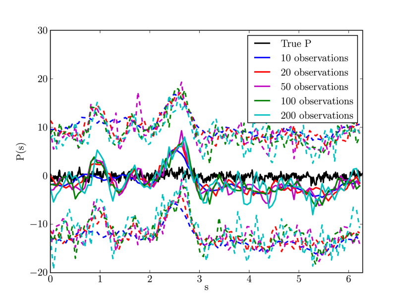
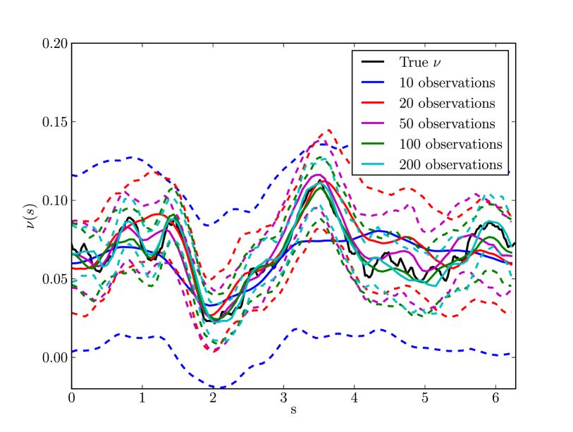
Figure 2 shows plots representing the mean and variance of the approximation of the functions $p_{0}$ (left) and $\nu$ (right) given an increasing number of observations. As the number of observations is increased, the better we recover the actual value of $\nu$ that was used to create the data, and the level of uncertainty in the distribution is reduced. The convergence of $p_{0}$ is not so clear, as the convergence is not expected to be pointwise in this case, but in $L^{2}(S^{1})$.

Figure 3: (a) Plots of the deformed shapes using the mean values of $p_{0}$ from Figure 2. (b) Marginal distribution of observational noise variance in the MCMC chains.

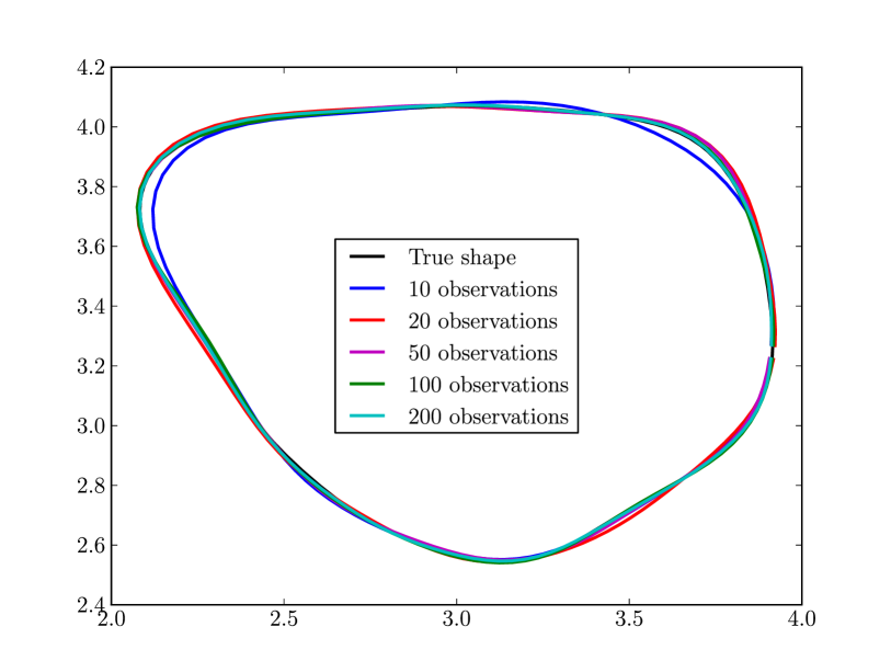
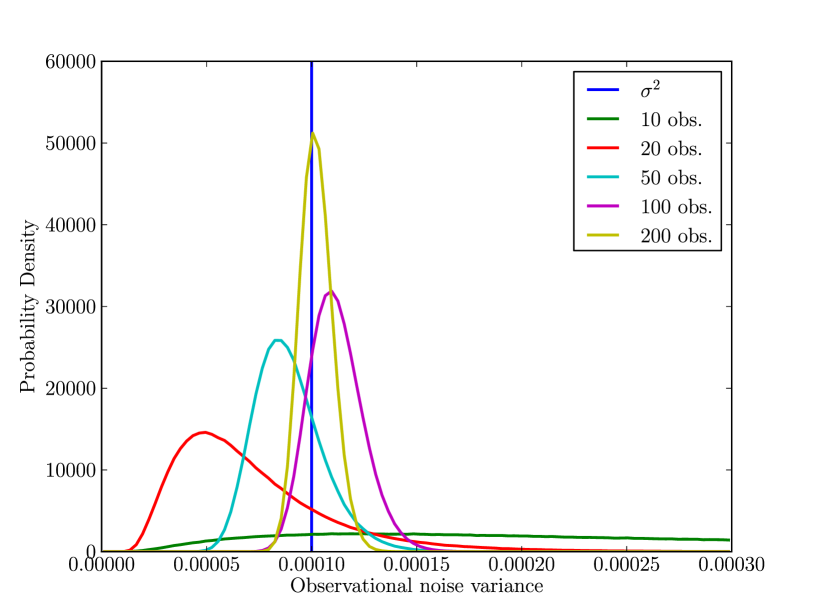
However, we can look at the deformed shapes that are produced by the mean initial momenta $\partial_{0}$ shown in Figure 2. These are shown in Figure 3 (left). The marginal distributions on the observational noise variance as estimated by the MCMC methods are plotted in Figure 3 (right). These clearly show that as the number of observations increases, the distribution is becoming increasingly peaked around the value that was used when creating the data.

7.2 Effect of lengthscale on multimodality

One might ask what the advantage of full posterior sampling is over other less computationally expensive optimisation approaches. In this section we show that certain data scenarios can cause the posterior distribution on the initial momentum $p_{0}$ to be complex with many local maxima of probability density. In this case the solution from an optimisation approach may not be unique, depending on the initial state of the solver. Being able to characterise the whole of the distribution in this case allows us to identify several different possibilities for the function $p_{0}$, and to get a better idea of the uncertainty in the problem. One such data scenario that exhibits this posterior multimodality is where we have features in the data whose lengthscale is smaller than the filtering lengthscale $\alpha$ in the metric for the diffeomorphism, as we demonstrate in the following example. Let us once again set the initial shape $\Gamma^{1}$ to be that defined by the parameterisation $p^{A}(s)$ given in (29). We then define $\Gamma^{2}(r)$ for $r\in[0,1]$, such that it consists of a square of length 2, centred at $[\pi,\pi]$, with quarter-circles of radius $r$ continuously added on each corner.

Figure 4: Plot of the target shape with varying $r$, the radius of the quarter circles on the corners of the square.

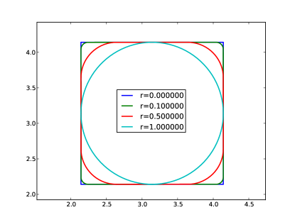
Figure 4 shows the target shape for a range of radii $r$. Note that for $r=0$, the shape is exactly a square of length 2, and for $r=1$ the shape is a circle of radius 2, exactly overlapping the template shape (29). The variable $r$ defines the minimum lengthscale of features in the data. Once $r$ becomes smaller than the maximum lengthscale than can be resolved by the model, we would expect to see multimodality creeping into the posterior distribution on $p_{0}$. Since the template shape cannot be bent to imitate the features on such a small scale, near to this feature only some of the observation points can be well-matched for any given $p_{0}$. This problem does not cause multimodality in the posterior distribution on the reparameterisation function $\nu$ since the observation points on the template shape do not need to move in order to minimise the distance between themselves and the observations for any of the possible $p_{0}$ configurations in the multimodal posterior on the initial momentum.

In the following experiments we look at what happens to the posterior distribution on $(p_{0},\nu)$ as $r$ starts at 1 and steadily decreases. For each value of $r$, we consider the shape $\Gamma^{2}(r)$ as described above, and place $10^{3}$ observation points along the shape, evenly spaced in terms of arc length. A large number of observations are used so that the data can resolve small lengthscales. We use these observation points as our data, with no noise added, to isolate the cause of the multimodality purely to the lengthscale of the features in the data. For the function $\Phi=\frac{1}{2}\|\mathcal{G}(p_{0},\nu)-y\|^{2}_{\Sigma}$ in the likelihood functional, we pick $\Sigma=\sigma^{2}I$ with $\sigma=10^{-2}$.

(a)

(b)

Figure 5: Plot of marginal distributions on (a) the lowest, (b) the second lowest wave number Fourier mode of the initial momentum function $p_{0}$, given varying value of $r$, the radius of the quarter circles in the target shape.

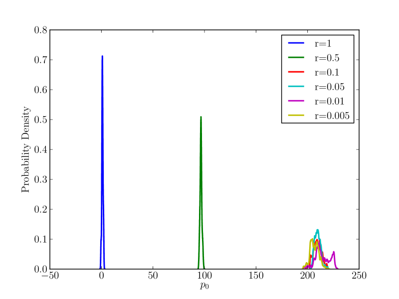
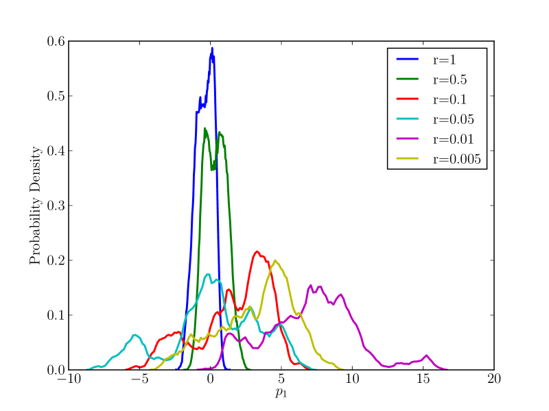
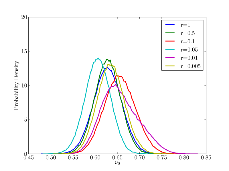
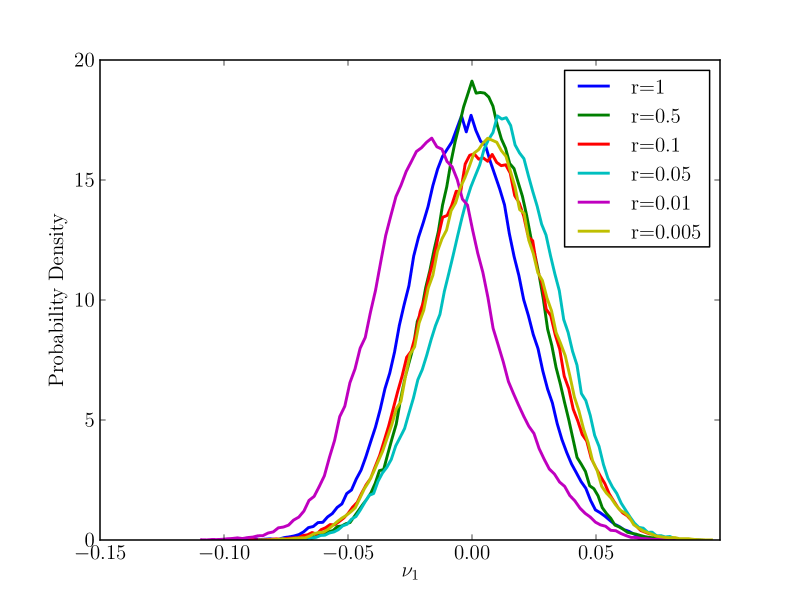
Figure 5 shows the marginal distributions on the first two Fourier modes of the initial momentum $p_{0}$ as the radius of the quarter circles in the data is reduced. Notice that for $r=1$, where the data is simply a circle, the distributions are smooth, monomodal and bell-shaped. However, as $r$ is reduced, the distributions become increasingly irregular, and in some cases multimodal. Moreover, these later examples take a great deal of time to converge as the posterior distribution is more complex, and it is harder to be sure that we have adequately explored the whole of the probability measure. However, these results show that the posterior measures arising from this application are non-Gaussian, and not necessarily monomodal. Simply finding the local maxima of probability density for these examples would not be a good description of the nature of the distribution as a whole, not would it help us in determining the uncertainty in the problem.

(a)

(b)

Figure 6: Plot of marginal distributions on (a) the lowest, (b) the second lowest wave number Fourier mode of the reparameterisation function $\nu$, given varying value of $r$, the radius of the quarter circles in the target shape.

Similarly, Figure 6 shows the marginal distributions on the first two Fourier modes of the reparameterisation function $\nu$ as the radius of the quarter circles in the data is reduced. Note that the distributions on $\nu$ are monomodal in nature, in contrast to those on $p$ in this data scenario.

7.3 Partial observations

Another area of interest to many practitioners is algorithms which try to recover information in the case where our observations of the target shape are only partial. We may only observe part of the shape, or our observations in some regions of the shape may be essentially destroyed by excessive noise. In this case we would expect to find many different possible shapes which could fit with our data equally well, meaning that the uncertainty quantification through full sampling of the Bayesian posterior is informative.

Let us consider the scenario where we have 1000 fairly evenly spaced observations of the target shape, where the template shape is given by (29) and where the functions $(p_{0},\nu)$ that create the target shape and the positions of the observation points are draws from the prior. Suppose now that the observation noise is no longer i.i.d. around the entire shape, but instead we have two regions with different covariance structure. In one region, covering approximately three quarters of the shape’s circumference, the noise is relatively small, distributed as $\mathcal{N}(0,\Gamma)$ with $\Gamma=\sigma_{D}^{2}I$ with $\sigma_{D}=0.0001$. In the final quarter of the domain we add noise with much larger variance, with $\sigma_{L}=0.1$. This value is so large that most of this data is rendered useless, in terms of extrapolating information about the value of the functions $p_{0}$ and $\nu$. As in Section 7.1, a very fine resolution of the curve was used when simulating the data (1000 points), and a coarser representation was used within the MCMC method (100 points).

In this data scenario, we must also be careful in our choice of functional $\Phi(p_{0},\nu)=\frac{1}{2}\|\mathcal{G}(p_{0},\nu)-y\|^{2}_{\Gamma_{\mbox{\tiny PO}}}$ in the likelihood. If we were to set $\Gamma_{\mbox{\tiny PO}}=\sigma_{D}^{2}$ over the whole domain, then we would be attempting to fit the shape very closely to the very noisy observations in the final third, which would cause all manner of problems. On the other hand, if we were to take $\Gamma_{\mbox{\tiny PO}}=\sigma_{L}^{2}$, we would be assuming a lot more uncertainty in the majority of the observations than is actually the case. In the numerics that follow, as we did in Section 7.1, we treat the observation noise variance $\sigma^{2}$ as an unknown also to be found.

Figure 7: Plot of partial data, due to large noise variance in one region of the observed shape. Green line denotes the converged solution of the corresponding optimisation problem.

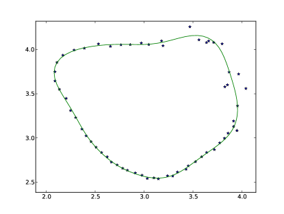
Figure 7 shows an example of such a data scenario. The stars denote data points, and the green curve denotes the converged solution of the corresponding optimisation problem as described in Section 5.1. However, this single curve does not tell us the whole story, since there are many curves that could satisfy the data (almost) as well as this curve.

Figure 8: Plot of 20 shapes arising from samples from the posterior distribution using the data plotted in 7 alongside (a) the data points, (b) the true shape (black curve). Since the recovered noise model assumes uniform observational noise over the whole shape, there is higher variability over the whole shape due to the extra noise in 1/4 of the data.

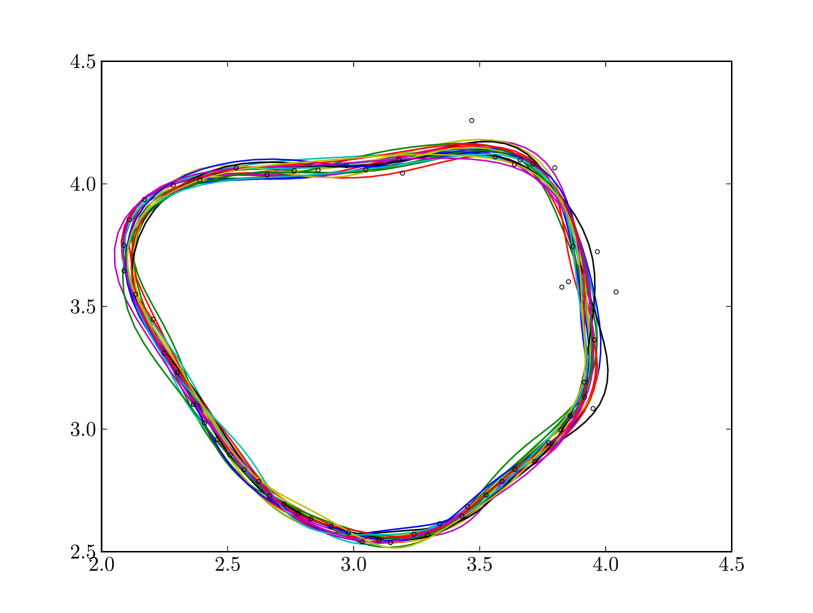
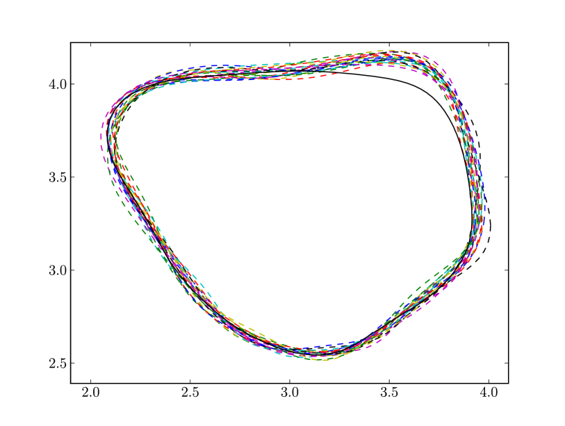
Figure 8 represents this variability through the plots of 20 shapes arising from samples of the posterior distribution using this data. The data is very poor in one region, and as such there are several shapes which match the data equally as well. The data is so poor in this one region that the recovery of the true shape in this area is poor.

(a)

(b)

Figure 9: Plots of the mean values (solid lines) of (a) $p_{0}$ and $\nu$ occurring in the posterior distribution using the data plotted in 7. The dashed lines denote $\pm 3$ standard deviations (approximately 99.7% confidence interval)

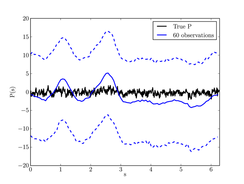
This variability can also be seen in Figure 9, where the mean and variance of the functions $p_{0}$ and $\nu$ in posterior distribution are visualised.

Figure 10: Marginal distribution of observational noise variance in the MCMC chain, using data plotted in 7. The two different variances used when creating the data are also shown.

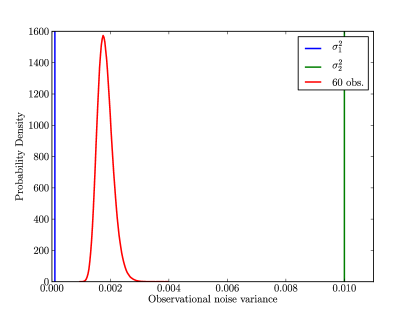
Figure shows the marginal distributions on the observational noise variance as estimated by the MCMC methods. The non-uniformity of the noise used when creating the data cannot be recovered in this setting since we assume uniformity over the whole shape in our prior on the observational noise variance. Therefore, the recovered values are somewhere between the poor and good SNR regimes. Note that in comparison with the distributions in Figure 2, the variances in these distributions are quite similar, despite having a great deal more observations. With a region with a much poorer SNR, the uncertainty in the system is much greater, and as such there is still a large region of the state space with similar probability density. The approach we have used in this paper allows us to quantify this uncertainty as well as finding states of maximal likelihood.

8 Conclusions

This paper presents a Bayesian approach to shape registration which takes into account the fact that observations of a shape are not exact, and gives a distribution on the shortest distance in shape space between the template shape to the observed shape. We concentrate on the case of a finite number of observations of points from the target curve, and our approach makes use of the use of explicit reparameterisation variable as described in [11, 20]. The sampling method is framed on function space and so is robust under refinements of discretisation [16].

By careful analysis of the forward problem, we have been able to formulate a well-posed Bayesian inverse problem regarding shape matching of a curve with a set of noisy observations of another. We have shown that the likelihood function is Lipschitz continuous on a space which has full measure with respect to a specified choice of Gaussian prior measure. Using this, we have shown how to draw samples from well-defined posterior distributions using the pCN MCMC sampler on function space. This choice of algorithm prevents slower convergence of the statistical algorithm as the discretisation of the observation operator is refined. We have then implemented this algorithm, and presented briefly some illustrative numerics.

In these numerics, we first showed that the posterior distribution shows consistency as the number of observations of a recoverable shape are increased, and the posterior distributions on the functions of interest become increasingly peaked on the functions which were used to create the data. We also showed an example, where the lengthscale of features in the data is small, in which the posterior distributions exhibit multimodal behaviour, indicating that full characterisation of the posterior can give us more information than the solution of an equivalent optimisation problem. Since the shape space is a Riemannian manifold with regions of positive and negative curvature, there may be more than one geodesic between two points in shape space, which may also lead to multimodality.

Finally we showed that this method can give us a range of different possible solutions in the case of lost or destroyed data for some part of the target shape.

Since we already have at our disposal an implementation of the adjoint problem so that we can calculate the gradient of the observation operator (which we use in the BFGS method for the deterministic burn-in), we can very simply adapt the MCMC method from random walk to a gradient method, such as the Metropolis Adjusted Langevin Algorithm (MALA). This would increase the efficiency of the algorithm markedly. Further analytical results would be needed, however, to ensure that the gradient of the observation operator is continuous on a space which has full measure with respect to an appropriately chosen prior distribution.

Another extension of this work would be to also make the problem translation, rotation and scale invariant, so that any misalignment of the imaging equipment has a negligible effect on the results. This would involve adding parameters into the state space to allow for these types of operations. One might also consider the case where the template shapes themselves are only noisily observed, so that we are trying to find a distribution on the length of geodesic paths in shape space between two noisily observed shapes. The problem could also be extended to the case in which the ordering of the observed points around the curve is not known, in which case the discrete ordering would also have to be learned as part of the inverse problem. This could be done by combining the present approach with a Gibb’s sampler for the ordering. This would result in a Bayesian approach to the segmentation process, in which points on the boundary between two materials might first be estimated from a bitmapped image but their ordering is not known with 100% confidence. The result would be a probability distribution on the boundary curve with some prescribed topology.

Acknowledgements The research leading to these results has received funding from the European Research Council under the European Community’s Seventh Framework Programme (FP7/2007-2013)/ ERC grant agreement No. 239870. This publication was based on work supported in part by Award No KUK-C1-013-04, made by King Abdullah University of Science and Technology (KAUST), and the results were obtained using the Imperial College High Performance Computing Centre cluster. SLC would also like to thank St Cross College Oxford for support via a Junior Research Fellowship.

References

- [1] M. I. Miller, A. Trouvé, and L. Younes. On the metrics, euler equations and normal geodesic image motions of computational anatomy. In Proceedings of the 2003 International Conference on Image Processing, volume 2, pages 635–638. IEEE, 2003.
- [2] M. I. Miller, A. Trouvé, and L. Younes. Geodesic shooting for computational anatomy. Journal of Mathematical Imaging and Vision, 24(2):209–222, 2006.
- [3] M. Vailliant, M. I. Miller, L. Younes, and A. Trouvé. Statistics on diffeomorphisms via tangent space representations. NeuroImage, 13:161–169, 2004.
- [4] P.T. Fletcher, C. Lu, S. M. Pizer, and S. Joshi. Principal geodesic analysis for the study of nonlinear statistics of shape. IEEE Transactions on Medical Imaging, 23(8):995–1005, 2004.
- [5] S. Allassonnière, Estelle Kuhn, , and Alain Trouvé. Construction of bayesian deformable models via stochastic approximation algorithm: A convergence study. Bernoulli, 16(3):641–678, 2010.
- [6] S. Allassonnière, Estelle Kuhn, and Alain Trouvé. Map estimation of statistical deformable template via nonlinear mixed effect models : Deterministic and stochastic approaches. Proc. of Mathematical Foundations of Computational Anatomy, 2008.
- [7] J. Ma, M.I. Miller, A. Trouvé, and L. Younes. Bayesian template estimation in computational anatomy. NeuroImage, 42(1):256–261, 2008.
- [8] D. D. Holm, J. T. Ratnanather, A. Trouvé, and L. Younes. Soliton dynamics in computational anatomy. NeuroImage, 23, Supplement 1:S170 – S178, 2004.
- [9] J. Glaunes, A. Trouvé, and L. Younes. Diffeomorphic matching of distributions: A new approach for unlabelled point-sets and sub manifolds matching. Proceedings of the 2004 IEEE Computer Society Conference on Computer Vision and Pattern Recognition.
- [10] Marc Vaillant and Joan Glaunes. Surface matching via currents. In IPMI, pages 381–392, 2005.
- [11] C.J. Cotter and D.D. Holm. Geodesic boundary value problems with symmetry. J. Geom. Mech., 2:51–68, 2010.
- [12] A. M. Stuart. Inverse problems: A bayesian perspective. Acta Numerica, 19:451–559, 2010.
- [13] S.L. Cotter, M. Dashti, J.C. Robinson, and A.M. Stuart. Bayesian inverse problems for functions and applications to fluid mechanics. Inverse Problems, 25, 2009.
- [14] S. L. Cotter, M. Dashti, and A. M. Stuart. Approximation of Bayesian inverse problems for PDEs. SIAM J. Numer. Anal., 48(1):322–345, 2010.
- [15] S. L. Cotter, M. Dashti, and A. M. Stuart. Variational data assimilation using targetted random walks. International Journal for Numerical Methods in Fluids, pages n/a–n/a, 2011.
- [16] S.L. Cotter, G.O. Roberts, A.M. Stuart, and D. White. MCMC methods for functions: modifying old algorithms to make them faster. Submitted to Statistical Science, 2012.
- [17] M. T. Miller and L. Younes. Group actions, homeomorphisms, and matching: A general framework. International Journal of Computer Vision, 41:61–84, 2001.
- [18] J. Glaunes, A. Trouvé, and L. Younes. Diffeomorphic matching of distributions: A new approach for unlabelled point-sets and sub-manifolds matching. In IEEE Computer Society Conference on Computer Vision and Pattern Recognition, volume 2, pages 712–718, 2004.
- [19] F. Gay-Balmaz and T.S. Ratiu. Clebsch optimal control in formulation in mechanics. J. Geom. Mech., 3(1), 2011.
- [20] C.J. Cotter, A. Clark, and J Peiró. A reparameterisation-based approach to geodesic shooting for curve matching. Int. J. Comp. Vis., pages 1–19, 2012. doi:10.1007/s11263-012-0520-0.
- [21] B. Khesin and R. Wendt. Geometry of infinite-dimensional groups, volume 51 of Ergebnisse der Mathematik und Grenzgebiete 3.Folge, chapter 1. Springer-Verlag, 2008.
- [22] C.G. Broyden. The convergence of a class of double-rank minimization algorithms. J. Inst. Maths Applics, 6:76–90, 1970.
- [23] D.F. Shanno. On Broyden-Fletcher-Goldfarb-Shanno method. J. Optimiz. Theory Appl., 46, 1985.
- [24] C. J. Cotter. The variational particle-mesh method for matching curves. J. Phys. A: Math. Theor., 41:344003, 2008.
- [25] S. Agapiou, S. Larsson, and A. M. Stuart. Posterior consistency of the bayesian approach to linear ill-posed inverse problems. arXiv:1203.5753v2.
- [26] B. T. Knapik, A.W. van der Vaart, and J. H. van Zanten. Bayesian inverse problems with Gaussian priors. Annals of Statistics, 39(5):2626–2657, Oct 2011.
- [27] B. T. Knapik, A. W. van der Vaart, and J.H. van Zanten. Bayesian recovery of the initial condition for the heat equation. Comm. Statist. Theory Methods, To appear.
- [28] J. Kaipio and E. Somersalo. Statistical and Computational Inverse Problems, chapter 2. Springer, 2004.