MOSE: zooming on the Meso-NH mesoscale model performances at the surface layer at ESO sites (Paranal and Armazones)

Abstract

In the context of the MOSE project, in this contribution we present a detailed analysis of the Meso-NH mesoscale model performances and their dependency on the model and orography horizontal resolutions in proximity of the ground. The investigated sites are Cerro Paranal (site of the ESO Very Large Telescope - VLT) and Cerro Armazones (site of the ESO European Extremely Large Telescope - E-ELT), in Chile. At both sites, data from a rich statistical sample of different nights are available - from AWS (Automated Weather Stations) and masts - giving access to wind speed, wind direction and temperature at different levels near the ground (from 2 m to 30 m above the ground). In this study we discuss the use of a very high horizontal resolution ($\Delta$X=0.1 km) numerical configuration that overcomes some specific limitations put in evidence with a standard configuration with $\Delta$X=0.5 km. In both sites results are very promising. The study is co-funded by ESO and INAF.

1 INTRODUCTION

This work is part of the MOSE (MOdeling ESO Sites) project, a feasibility study for the turbulence prediction at two ESO Sites: Cerro Paranal (site of the VLT) and Cerro Armazones (future site of the E-ELT). One of the main goal of the MOSE project is to supply a tool for optical turbulence forecasts to support the scheduling of the scientific programs and the use of AO facilities at the VLT and at the E-ELT. In a joint paper, Masciadri & Lascaux [1] have presented the results of numerical simulations of 20 different summer nights (in November and December 2007) with the mesoscale model Meso-NH [2] with a standard configuration using 3 imbricated domains with the innermost horizontal resolution equal to $\Delta$X=0.5km. The results are already very encouraging, especially in the free atmosphere, with a good prediction of the meteorological parameters important to the optical turbulence estimation (temperature, wind speed). The main discrepancies concerning the meteorological parameters between Meso-NH predictions and observations have been identified near the surface (between 2 m and 30 m above the ground), for the wind speed. To overcome these specific limitations of the standard configuration, we discuss in this study the impact of the use of a higher horizontal resolution numerical configuration. Two domains with a horizontal resolution equal for both to $\Delta$X=0.1km, centered above Cerro Paranal and Cerro Armazones, have been added. It is very important to well predict meteorological parameters such as wind speed and temperature, and their temporal evolution. Indeed, the intensity of the optical turbulence, characterized by the structure constant of the refractive index $C_{N}^{2}$, mainly depends on their values and gradients. Our team have already used so far the Meso-NH model to perform some meteorological, and optical turbulence, numerical simulations, at other sites ( San Pedro Martir [3], Mount Graham [4, 5], Antarctica [6, 7, 8]) discussing its abilities in predicting meteorological and astroclimatic parameters, but with less rich data samples.

2 OBSERVATIONS DATA-SET

Two sites are investigated in this study: Cerro Paranal, site of the ESO Very Large Telescope (VLT), and Cerro Armazones, future site of the ESO European Extremely Large Telescope (E-ELT). At Paranal, observations of meteorological parameters near the surface come from an automated weather station (AWS) and a 30 m high mast including a number of sensors at different heights. Both instruments are part of the VLT Astronomical Site Monitor [9]. Absolute temperature data are available at 2 m and 30 m above the ground. Wind speed data are available at 10 m and 30 m above the ground. At Armazones, observations of the meteorological parameters near the ground surface come from the Site Testing Database [10], more precisely from an AWS and a 30 m Tower (with temperature sensors and sonic anemometers). Data on temperature and wind speed are available at 2 m, 11 m, 20 m and 28 m above the ground. At 2 m, at Armazones, temperature measurements from the AWS and the sonic anemometers are both available but we consider only those from the tower (accuracy of 0.1${}^{o}C$ [11]). Those from the AWS are not reliable because of some drift effects (T. Travouillon, private communication). Wind speed observations are taken from the AWS (at 2 m) and from the sonic anemometers of the tower (at 11 m, 20 m and 28 m). The outputs are sampled at 1 minute intervals.

Figure 1: Orography (altitude in m) of the region of interest as seen by the Meso-NH model (polar stereographic projection) for all the imbricated domains of the grid-nested configuration. (a) Domain 1 (orographic data from GTOPO), (b) Domain 2 (orographic data from GTOPO), (c) Domain 3 (orographic data from ISTAR), (d) Domain 4 (orographic data from ISTAR), (e) Domain 5 (orographic data from ISTAR), A dot stands for Cerro Armazones and P dot stands for Cerro Paranal. See Table 1 for the specifications of the domains (number of grid-points, domain extension, horizontal resolution).

3 MESO-NH MODEL CONFIGURATION

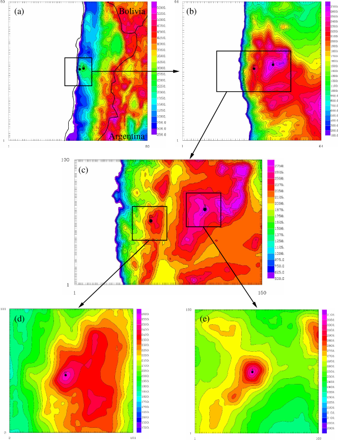
All the numerical simulations of the nights presented in this study are performed with the mesoscale numerical weather model Meso-NH [2]. The Meso-Nh model can simulate the temporal evolution of three-dimensional meteorological parameters over a selected finite area of the globe. The system of hydrodynamic equations is based upon an anelastic formulation allowing for an effective filtering of acoustic waves. It uses the Gal-Chen and Sommerville[13] coordinates system on the vertical and the C-grid in the formulation of Arakawa and Messinger[14] for the spatial digitalization. It employs an explicit three-time-level leap-frog temporal scheme with a time filter [15]. It employs a one-dimensional 1.5 turbulence closure scheme [16]. For this study we use a 1D mixing length proposed by Bougeault and Lacarrère [17]. The surface exchanges are computed using ISBA [18] (Interaction Soil Biosphere Atmosphere). The grid-nesting technique [19], employed in our study, consists of using different imbricated domains of the Digital Elevation Models (DEM i.e orography) extended on smaller and smaller surfaces, with increasing horizontal resolution but with the same vertical grid. Two different grid-nesting configurations have been employed. The standard configuration includes three domains (domains 1, 2 and 3 from Figure 1 and Table 1) with the lowest horizontal resolution equal to 10 km and the highest horizontal resolution equal to 0.5 km. The second configuration is made of five imbricated domains, the first same three as the previous configuration, and other two centered at both Paranal and Armazones sites, with a horizontal resolution of $\Delta$X=0.1 km (thereafter ”5dom” configuration - domains 1, 2, 3, 4 and 5 from Figure 1). One can notice that using these configurations, we are able to do the forecast at both sites simultaneously. The orographic DEMs we used for this project are the GTOPO with an intrinsic horizontal resolution of 1 km (used for the domains 1 and 2) and the ISTAR with an intrinsic horizontal resolution of 0.5 km (used for the domain 3, 4 and 5). Along the z-axis we have 62 levels distributed as follows: a first vertical grid point equal to 5 m, a logarithmic stretching of 20 $\%$ up to 3.5 km above the ground, and an almost constant vertical grid size of $\sim$600 m up to 23.8 km. The model has been parallelized using OPEN-MPI-1.4.3 and it run on local workstations as well as on the HPCF cluster of the European Centre for Medium weather Forecasts (ECMWF). The second solution permitted us to achieve relatively rich statistical estimates of these analysis.

All simulations were initialized the day before at 18 UT and forced every 6 hours with the analyses from the ECMWF, and finished at 09 UT of the simulated day (duration: 15 hours). The statistics we deal with in the next sections was computed only during night time, from 00 UT to 09 UT.

Table 1: Meso-NH model configuration. In the second column the horizontal resolution $\Delta$X, in the third column the number of grid points and in the fourth column the horizontal surface covered by the model domain.

Domain	$\Delta$X	Grid Points	Surface
	(km)		(km$\times$km)
Domain 1	10	80$\times$ 80	800$\times$800
Domain 2	2.5	64$\times$ 64	160$\times$160
Domain 3	0.5	150$\times$100	75$\times$50
Domain 4	0.1	100$\times$100	10$\times$10
Domain 5	0.1	100$\times$100	10$\times$10

Table 2: Peak resolution with respect to the orographic model and the Meso-NH horizontal resolution. GTOPO is the standard digital elevation model (DEM), from the US Geological Survey, used by the Meso-NH model. It is not used in this study for the high-resolution domains (from domain 3 to 5), but we remind it here for comparisons purpose. ISTAR is the DEM used in this study for both 3dom and 5dom configurations in the innermost domains. SRTM (Shuttle Radar Topography Mission) is a more recent DEM with a higher intrinsic resolution [20], that we planned to implement in further studies. $\Delta$h represents the difference between the real altitude of the peak and the altitude of the peak in Meso-NH.

Orographic	Intrinsic	Meso-NH	Paranal	Armazones
model	resolution	horizontal resolution	$\Delta$h	$\Delta$h
GTOPO	1km	500m	204m	245m
ISTAR	500m	500m (3dom)	156m	164m
ISTAR	500m	100m (5dom)	89m	55m
SRTM	90m	100m	5m	26m

4 COMPARISON MESO-NH OUPTUT vs OBSERVATIONS

In a joint paper [1] our team presented the results of Meso-NH simulations in the standard configuration for simulations at Cerro Paranal and Cerro Armazones. The results were already very encouraging. However, the performances concerning the prediction of the meteorological parameters in proximity of the ground were mitigated. The statistics was performed on 20 nights, using two statistical operators beside the average: the bias and the root mean square error (RMSE). The prediction of the absolute temperature was very good. At the 2 m and 30 m levels for Cerro Paranal, and at the 2 m, 11 m, 20 m and 28 m levels at Cerro Armazones, the biases between observations and model output were inferior to 1${}^{o}C$. The RMSE was equal, or slightly inferior to, $\sim$1${}^{o}C$. These are very good values. On the contrary, the prediction of the wind speed above the surface was strongly underestimated by the model with respect to the observations, especially at the closest levels near the ground. For example, at Cerro Armazones the bias reached $\sim$-3.6 $m{\cdot}s^{-1}$ at 2 m, with a RMSE equal to $\sim$4.6 $m{\cdot}s^{-1}$.

To quantify the gain in statistic reliability, obtained with a very high horizontal resolution, in reconstructing surface meteorological parameters, the bias and the RMSE of the nightly temporal evolutions of temperature and wind speed have been computed, at each level where observations were available. In the study presented here, a set of 9 nights (for Cerro Paranal) and 5 nights (for Cerro Armazones) have been simulated with the Meso-NH model both with the 3dom and 5dom configurations presented in the previous section. This is a preliminary and ongoing work on the influence of the very high horizontal resolution ($\Delta$X=0.1km) on the prediction of meteorological parameters in proximity of the ground. That’s why the number of investigated nights is not the same than in Masciadri & Lascaux [1], and different for the two sites (it also depends on the available observations for a given day). However it is planned to extend it to better validate the results.

4.1 Wind and temperature temporal evolutions - mean, bias and RMSE

In this section we present the average, bias and RMSE of the nightly temporal evolution of wind speed and temperature at Cerro Paranal and Cerro Armazones. The average, the bias and the RMSE between simulated and observed parameters are defined as:

$$AVERAGE=\sum_{i=1}^{N}\frac{X_{i}}{N}$$

$$BIAS=\sum_{i=1}^{N}\frac{(Y_{i}-X_{i})}{N}$$

$$RMSE=\sum_{i=1}^{N}\sqrt{\frac{(Y_{i}-X_{i})^{2}}{N}}$$

with $X_{i}$ beeing the observed values and $Y_{i}$ the simulated values. $N$ is the total number of times in which the couple ($X_{i}$,$Y_{i}$) is available and different from zero. In the case of the comparisons of the temporal evolutions (Figures 2, 3, 4 and 5), $N\leq n$, with $n$ the number of nights, which simply means that observed values are not always available at every minutes for every nights and in these cases the statistics is performed on a number of points inferior to the total number of nights. In the case of Tables 3 and 4, N represents the total number of available measurements, for all the nights considered.
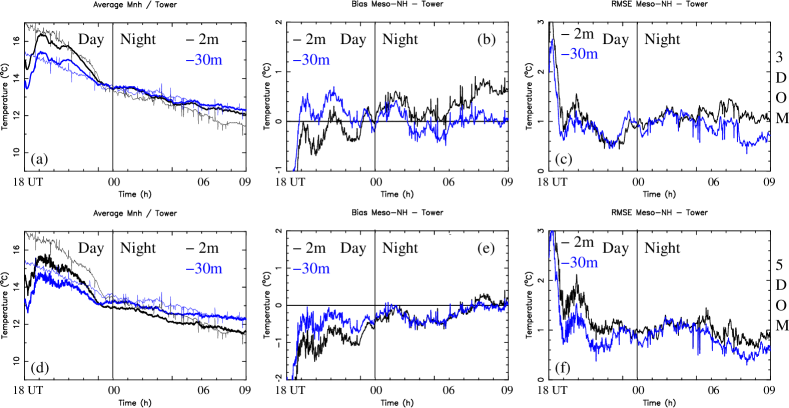
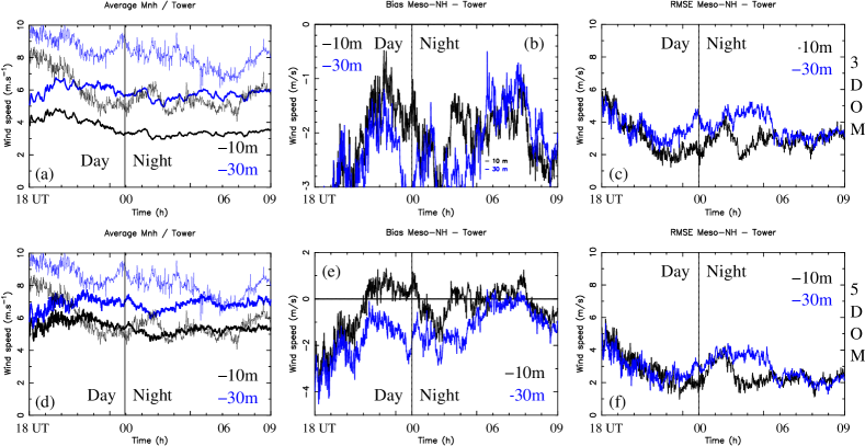
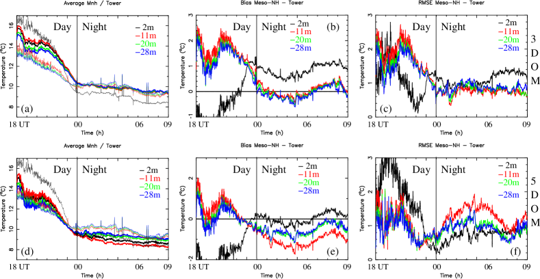
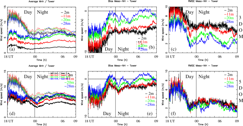
The temporal evolutions of the average, bias and RMSE for both 3dom and 5dom configurations, are displayed on Figures 2 and 3 at Cerro Paranal (temperature and wind speed, respectively) and Figures 4 and 5 at Cerro Armazones (temperature and wind speed, respectively).
A summary of the values of bias and RMSE are reported on Tables 3 and 4, for temperature and wind speed, respectively. It permits us to quantify the gain obtained in the prediction of the temperature and wind speed near the ground, going from an horizontal resolution equal to $\Delta$X=0.5km (3dom) to $\Delta$X=0.1km (5dom). We focus our attention on nightly values only, as in Masciadri & Lascaux [1]. The first 6 hours of simulation, during daytime, are affected by sone spurious values due to the adaption of the model to the orography, especially during the first part of the simulation.

The first important thing to notice is that the statistics on temperature remains good with the 5dom configuration, as it was for the 3dom configuration. We have biases inferior, or very close to, 1${}^{o}C$, and RMSEs close to 1${}^{o}C$. Concerning the temperature prediction by the model, one important feature was better reproduced with the 5dom configuration than with the 3dom configuration. The observed temperature gradient during night time between 2 m and the successive levels was almost absent with the 3dom configuration (Figures 2a and 4a). The 5dom configuration was able to better reproduce it, at Cerro Paranal and at Cerro Armazones (Figures 2d and 4d). In particular the prediction of the inversion of the vertical gradient of temperature near the surface, during the passage from day to night (from negative to positive), is improved in the 5dom simulations. However, as it was shown for the standard 3dom configuration [1], the 11 m level at Armazones still presents a wrong gradient tendency with the 5dom configuration.

Concerning the wind speed, there was a strong understimation of its intensity with the standard 3dom configuration, especially at the first 2 m level. It seems that the Meso-NH model isn’t able to reproduce high wind in proximity of the ground, at the peaks, with the 3dom configuration, leading to high values of bias and RMSE. This problem is partially solved with the 5dom configuration, where the model is now able to produce high winds even for the first levels of the model at Cerro Paranal and Cerro Armazones. At 10 m at Cerro Paranal for example, the bias is strongly reduced (cf. Table 4), from -2.07 $m{\cdot}s^{-1}$ to -0.16 $m{\cdot}s^{-1}$. Biases at 30 m at Cerro Paranal, at 2 m, 11 m and 20 m at Cerro Armazones are more than halved, having now values smaller than for the 3dom configuration: for the 3dom configuration, they are between -2 $m{\cdot}s^{-1}$ and -5 $m{\cdot}s^{-1}$; for the 5dom configuration they are between -0.8 $m{\cdot}s^{-1}$ and -2 $m{\cdot}s^{-1}$. At 28 m at Cerro Armazones, the bias is even equal to 0 $m{\cdot}s^{-1}$, whereas it was close to -1 $m{\cdot}s^{-1}$ with the 3dom configuration. The RMSE values are reduced too. The strongest RMSE, at 2 m at Cerro Armazones, was equal to 5.72 $m{\cdot}s^{-1}$ with the 3dom configuration, it is now equal to 3.15 $m{\cdot}s^{-1}$ with the 5dom configuration. However, even though the prediction of the wind speed with the 5dom configuration is very good, one minor discrepancy still remains at Cerro Armazones. In the observations, a low level jet is visible at 11 m. This level exhibits the highest wind speed with respect to the others levels at 2 m, 20 m and 28 m. On the contrary, the wind speed is constantly increasing in the model from 2 m to 28 m, suggesting that the low level jet may be at slightly higher levels in the model than in the observations.

Table 3: Bias and RMSE of the temperature between Meso-NH simulations (3dom and 5dom configurations) and observations, at Cerro Paranal (left) and Cerro Armazones (right). Units in ${}^{o}C$. Computations are made with 9 nights for Paranal and 5 nights for Armazones.

PARANAL		2 m	30 m	ARMAZONES		2 m	11m	20 m	28 m
(9 nights)				(5 nights)
3dom	BIAS	0.37	0.00	3dom	BIAS	0.84	0.06	-0.03	-0.08
	RMSE	1.13	0.92		RMSE	1.11	0.75	0.83	0.87
5dom	BIAS	-0.20	-0.22	5dom	BIAS	0.02	-1.04	-0.56	-0.53
	RMSE	1.00	0.85		RMSE	0.76	1.30	0.95	0.94

Table 4: Same as Table 3 but for the wind speed. Units in $m{\cdot}s^{-1}$.

PARANAL		10 m	30 m	ARMAZONES		2 m	11m	20 m	28 m
(9 nights)				(5 nights)
3dom	BIAS	-2.07	-2.16	3dom	BIAS	-4.78	-3.95	-1.97	-0.92
	RMSE	2.94	3.77		RMSE	5.72	5.10	3.34	2.49
5dom	BIAS	-0.16	-1.01	5dom	BIAS	-2.06	-1.92	-0.78	0.01
	RMSE	2.46	2.97		RMSE	3.15	3.21	2.50	2.49

Figure 2: 9 nights statistics on the temporal evolution of the temperature (in ${}^{o}C$) at Cerro Paranal at 2 m (in black) and at 30 m (in blue). (a) average with the 3dom configuration, (b) bias with the 3dom configuration, (c) rmse with the 3dom configuration, (d) average with the 5dom configuration, (e) bias with the 5dom configuration, (f) rmse with the 5dom configuration. The thin lines are observations averages. The thick lines are Meso-NH averages.

Figure 3: Same as Figure 2, but for wind speed (unit in $m{\cdot}s^{-1}$) at Cerro Paranal.

Figure 4: Same as Figure 2, but for temperature (in ${}^{o}C$) at Cerro Armazones.

Figure 5: Same as Figure 4, but for wind speed (unit in $m{\cdot}s^{-1}$) at Cerro Armazones.

4.2 Wind and temperature temporal evolutions - 11 November 2007

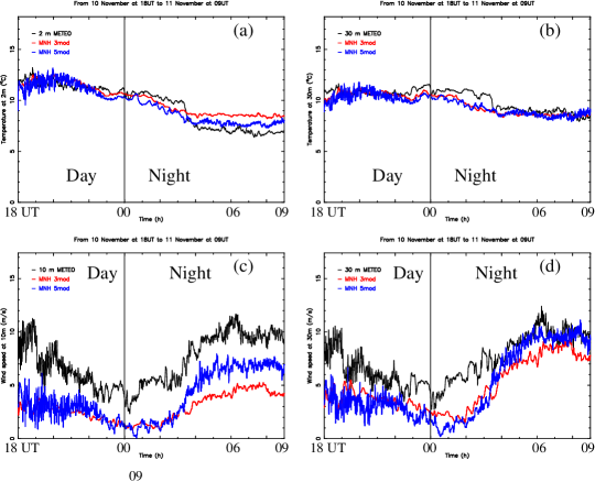
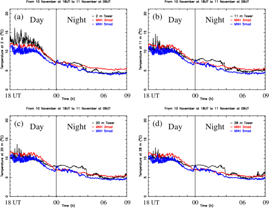
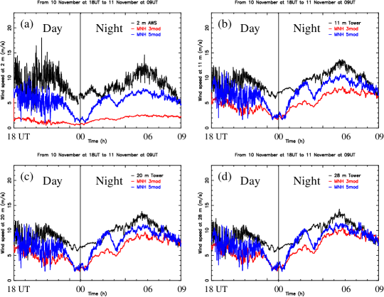
In this section we present the results for one night only, the 11 November 2007. It allows us to illustrate how good can be the improvements on the prediction of wind speed and temperature near the ground, for one single night, if we use a higher horizontal resolution. Figure 6 displays the temporal evolution of the temperature (top) and the wind speed (bottom) for this night, at Cerro Paranal, for both 3dom and 5dom configurations, and observations, at 2 m and 30 m for the temperature and at 10 m and 30 m for the wind speed. Figure 7 displays the temporal evolution of the temperature at Cerro Armazones for the same night, at four different levels (2 m, 11 m, 20 m, 28 m). Figure 8 displays the temporal evolution of the wind speed at Cerro Armazones for the same night, at four different levels (2 m, 11 m, 20 m, 28 m). At 2 m, the forecasted nightly temperature with the 3dom configuration was slightly warmer than the observations, for both sites. The difference is very small, smaller than 1.5${}^{o}C$ at Paranal and 1${}^{o}C$ at Armazones. At 30 m, at the end of the night, there is almost no bias between observations and forecast. Using the 5dom configuration, a small cooling appears with respect to the 3dom configuration, at 2 m, making the prediction almost perfect at this level. More over, the prediction at other levels m is not degraded (except for a very small cooling with respect to the observations at 11 m, 20 and 28 m at Cerro Armazones).

The major improvements brought by the highest horizontal resolution configuration can be seen for the wind speed. At Paranal, for this night, the wind speed reached around 10 $m{\cdot}s^{-1}$ at 2 m and 10 m. With the 3dom configuration, the wind speed at 2 m stalled at 5 $m{\cdot}s^{-1}$, whereas with the 5dom configuration it reached 7 $m{\cdot}s^{-1}$, closer to the observed 10 $m{\cdot}s^{-1}$. The prediction at 30 m with the 3dom configuration was satisfactory (around 8 $m{\cdot}s^{-1}$), but it is almost perfect at the end of the night with the 5dom configuration where it reached 10 $m{\cdot}s^{-1}$. The improvement is even more significative at Cerro Armazones at the first observed level (2 m). The observed wind speed oscillated during the night between 5 and 12 $m{\cdot}s^{-1}$. With the 3dom configuration, the first simulated level forecasted a wind speed always inferior at 2 $m{\cdot}s^{-1}$. Using the 5dom configuration, the forecasted wind oscillated between 5 and 8 $m{\cdot}s^{-1}$ (2 m). More over, the temporal evolution exhibits a peak of intensity at the exact same time (around 05:30 UT). This improvement in the wind speed forecast is visible also at the others 3 levels (11 m, 20 m, 28 m).

Figure 6: Temporal evolutions of (a) temperature at 2 m, (b) temperature at 30 m, (c) wind speed at 10 m and (d) wind speed at 30 m, at Cerro Paranal, for the night 11 November 2007. Units in ${}^{o}C$ for the temperature and in $m{\cdot}s^{-1}$ for the wind speed. In black, observations. In red, the 3dom simulation. In blue, the 5dom simulation.

Figure 7: Temporal evolutions of temperature (a) at 2 m, (b) at 11 m, (c) at 20 m and (d) at 28 m, at Cerro Armazones, for the night 11 November 2007. Units in ${}^{o}C$. In black, observations. In red, the 3dom simulation. In blue, the 5dom simulation.

Figure 8: Temporal evolutions of wind speed (a) at 2 m, (b) at 11 m, (c) at 20 m and (d) at 28 m, at Cerro Armazones, for the night 11 November 2007. Units in $m{\cdot}s^{-1}$. In black, observations. In red, the 3dom simulation. In blue, the 5dom simulation.

5 CONCLUSION

The intensity of the optical turbulence is mainly driven by the gradients of some meteorological parameters (wind speed, temperature) that determine the vertical profiles of $C_{N}^{2}$. As these vertical profiles of $C_{N}^{2}$, from which derive all the astroclimatic parameters useful for astronomers (seeing, wavefront coherence time, isoplanatic angle…) are characterized by a maximum in the surface layer, a good knowledge and prediction of the surface meteorological parameters is mandatory to obtain good forecast of the optical turbulence at a given site. In this study we have investigated the impact of very high horizontal resolution on the prediction of meteorological parameters (temperature and wind speed) near the surface at two montainous sites: Cerro Paranal (site of the VLT) and Cerro Armazones (future site of the E-ELT). In the standard configuration [1], less demanding in computing resources, the results are already very encouraging over the entire atmosphere above the sites of interest. Nevertheless, some discrepancies on the wind speed prediction near the ground were present, with low-level simulated winds lower than the obervations. The work presented in this study adressed this particular problem by testing a very high horizontal resolution configuration (5dom, with $\Delta$X=0.1km for the innermost domains), more demanding in computing resources. In this preliminary study (only 9 nights for Cerro Paranal and 5 nights for Cerro Armazones were investigated), we demonstrated that a very high horizontal resolution improved significatively the performance of the model in proximity of the ground. Concerning the temperature, not only the prediction of the low-level temperature remained very good (with biases inferior to 1${}^{o}C$ at all levels at both sites, and even equal to 0${}^{o}C$ at 2 m at Cerro Paranal), but the day to night temperature gradient inversion was more accurately reproduced. Concerning the wind speed, the comparison between 5dom simulations and observations gave biases reduced by more than a half at all levels, at both sites, with respect to the standard 3dom configuration.