Abstract

In this paper we apply digital in-line holography to image opaque objects through a thick plano-concave pipe. Opaque fibers and opaque particles are considered. Analytical expression of the intensity distribution in the CCD sensor plane is derived using generalized Fresnel transform. The proposed model has the ability to deal with various pipe shape and thickness and compensates for the lack of versatility of classical DIH models. Holograms obtained with a 12 mm thick plano-concave pipe are then reconstructed using fractional Fourier transform (FRFT). This method allows us to get rid of astigmatism. Numerical and experimental results are presented.

OCIS codes: 090.0090, 070.0070, 100.0100

1 Introduction

Digital in-line holography (DIH) is a recognized optical technique for flow measurements in transparent liquid media. This method is widely used in various domains such as fluid mechanics [1, 2] where the flow is seeded with small particles, or in the biological microscopic imaging field [3, 4]. Nevertheless, a transparent pipe can be viewed as an optical system that can introduce aberrations such as astigmatism [5]. These aberrations make difficult to image objects in the pipe. Compensation for these unwanted effects has been widely investigated. De Nicola et al. [6] proposed a numerical method to compensate for anamorphism. By modifying the chirp function and the spatial frequency term of the Fresnel integral the authors managed to compensate for a severe anamorphism brought by a reflexion diffraction grating. Numerical methods for astigmatism compensation have been proposed in Refs. [6, 7, 8]. Here the authors used a modified chirp function where two different propagation distances are considered. Astigmatism can also be compensated for by optical means. For instance, the authors of [9] used index matching to minimize astigmatism: the thin-lens like effect of an ampule filled with contaminants was investigated to determine index matching parameters for astigmatism compensation. However, the pipe used to carry a flow must be considered as a thick and cylindrical optical system. Recently, an analytical solution of the scalar diffraction produced by an opaque disk illuminated by an elliptical, astigmatic and Gaussian beam under Fresnel approximation has been proposed [10]. In this publication, the astigmatism was introduced and controlled by using a thin plano-convex cylindrical lens. Using fractional Fourier transformation (FRFT), authors managed to retrieve a correct image of an opaque disk from astigmatic hologram. It was shown that FRFT is therefore well suited for these studies where classical methods such as Fresnel transform [11] or Wavelet transform [12] fail.

The astigmatism introduced by thin lenses is thus well controlled. However, these DIH models can not be applied to hugger pipes. As a matter of fact, the optical thickness of these has to be taken into account.

In this paper, the aim is to apply DIH to thick pipe systems. In the first part of the paper, the intensity distribution, in the CCD plane, of the diffracted field produced by an opaque object located in a pipe is calculated. A method of Gaussian functions superposition is used to describe the object function. In the second part, definition of the FRFT is recalled and we demonstrate its ability to reconstruct holograms recorded in such systems. Finally simulations and experiments are performed to illustrate our results.

2 In-line Holography through pipes

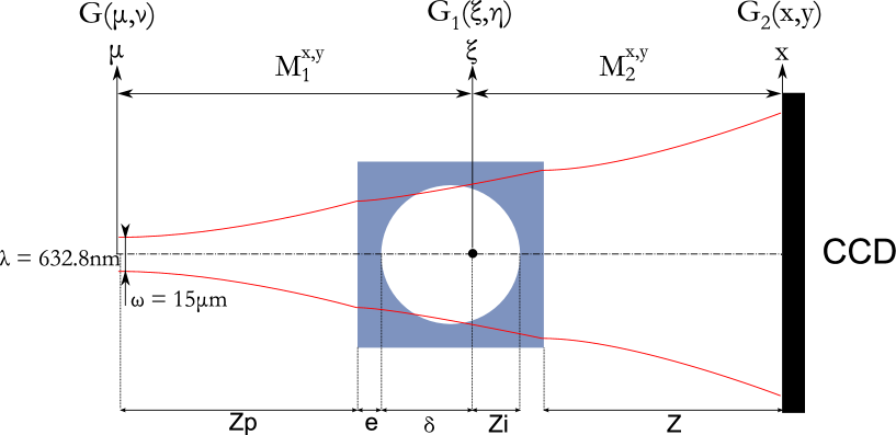
Holography aims to record, on a CCD camera without objective lens, the intensity distribution of the diffraction pattern of an object illuminated by a monochromatic continuous wave [13]. The numerical and experimental set-up is represented in Fig. (1). The incident Gaussian beam propagates in free space over a distance $z_{p}$ and illuminates the pipe. Here, the pipe is modeled as two thick lenses. Their thickness is denoted by $e$. The opaque object is located between these two lenses: at a distance $\delta$ from the first thick lens, and at a distance $z_{i}$ from the second lens. The CCD sensor is located at the distance $z$ next the pipe and records the intensity distribution of the diffraction pattern.

2.A Intensity distribution in the CCD sensor plane

In this part, we consider the propagation of a Gaussian beam through our optical system. In the beam waist plane, located at a distance $-z_{p}$ from the pipe, the Gaussian beam, denoted $G$, is defined by:

$$G\left(\mu,\nu\right)=\exp\left(-\frac{\mu^{2}+\nu^{2}}{w^{2}}\right),$$ (1)

where $\omega$ is the waist width and $\left(\mu,\nu\right)$ are the coordinates in the beam waist plane.

The propagation of the Gaussian beam through the pipe, to the CCD sensor is decomposed into two steps. The first step is the propagation of the illuminating beam (i.e $G\left(\mu,\nu\right)$) from the beam waist plane to the front of the opaque object. Using the generalized Huygens-Fresnel integral [14, 15, 16], the amplitude of the field in the pipe, denoted $G_{1}$, is defined by:

$$G_{1}\left(\xi,\eta\right)=\frac{\exp\left(i\frac{2\pi}{\lambda}E_{1}\right)}{i\lambda\sqrt{B^{x}_{1}B^{y}_{1}}}\int_{\mathbb{R}^{2}}G\left(\mu,\nu\right)\exp\left[i\frac{\pi}{\lambda B^{x}_{1}}\left(A^{x}_{1}\mu^{2}-2\xi\mu+D^{x}_{1}\xi^{2}\right)\right]\\ \times\exp\left[i\frac{\pi}{\lambda B^{y}_{1}}\left(A^{y}_{1}\nu^{2}-2\eta\nu+D^{y}_{1}\eta^{2}\right)\right]d\mu d\nu,$$ (2)

$A^{x,y}_{1}$, $B^{x,y}_{1}$, $D^{x,y}_{1}$ are given by $M_{1}^{x,y}$ matrices of Eq. (38) in App. (A). To obtain the relation of the intensity distribution, the linear canonical transformation is used. For the basic definitions and properties of the linear canonical transformation, we refer to [17]. This transformation is a parameterized integral operator of parameters $A$, $B$, $C$ and $D$. Each parameter represents a coefficient of a transfer matrix denoted $M$ (Cf appendix A). In our case the Fresnel transform is considered [18, 19]. It should be noted that the values of the coefficients are different in both $\xi$ and $\eta$ direction. This is due to the cylindrical geometry of the pipe. The distance $E_{1}=z_{p}+e+\delta$ corresponds to the waist-object distance. Using the same formalism, the amplitude in the CCD plane, denoted $G_{2}\left(x,y\right)$, can be written as:

$$G_{2}\left(x,y\right)=\frac{\exp\left(i\frac{2\pi}{\lambda}E_{2}\right)}{i\lambda\sqrt{B^{x}_{2}B^{y}_{2}}}\int_{\mathbb{R}^{2}}G_{1}\left(\xi,\eta\right)\left[1-T\left(\xi,\eta\right)\right]\exp\left[i\frac{\pi}{\lambda B^{x}_{2}}\left(A^{x}_{2}\xi^{2}-2x\xi+D^{x}_{2}x^{2}\right)\right]\\ \times\exp\left[i\frac{\pi}{\lambda B^{y}_{2}}\left(A^{y}_{2}\eta^{2}-2y\eta+D^{y}_{2}y^{2}\right)\right]d\xi d\eta,$$ (3)

where the parameters $A^{x,y}_{2}$, $B^{x,y}_{2}$, $D^{x,y}_{2}$ are given by $M_{2}^{x,y}$ matrices of Eq. (39). The distance $E_{2}=z_{i}+e+z$ is the distance between the object and the CCD sensor.

The spatial transmittance of the opaque 2D-object is defined by $\left[1-T\left(\xi,\eta\right)\right]$. Here $T\left(\xi,\eta\right)$ can be expressed as a superposition of Gaussian functions [20, 21], such as:

$$T\left(r\right)=\sum_{k=1}^{N}A_{k}\exp\left(-r^{T}R^{T}P_{k}Rr\right),$$ (4)

with

$$R=\left(\begin{array}[]{cc}\cos\theta&\sin\theta\\ -\sin\theta&\cos\theta\\ \end{array}\right),$$ (5)

and

$$P_{k}=\left(\begin{array}[]{cc}\frac{B_{k}}{a^{2}}&0\\ 0&\frac{B_{k}}{b^{2}}\\ \end{array}\right).$$ (6)

This expression permits to deal with non symmetrical optical systems and elliptical opaque objects [22, 23, 24, 25]. This Gaussian decomposition is very convenient; as a matter of fact it allows us to establish analytical expression of the diffracted pattern in the CCD plane. It also allows us to simulate holograms of 3D opaque objects whose 2D projection is elliptic or circular [26] (e.g. spheroids, fibers …).

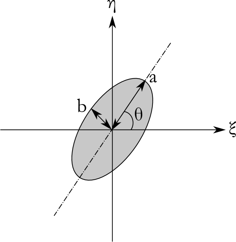
The object parameters are illustrated on Fig. (2). The coefficients $a$ and $b$ are the object radii within $\eta$ and $\xi$ axis respectively, $\theta$ is the angle between elliptical aperture principal axis and $\xi$ axis. The $A_{k}$ and $B_{k}$ coefficients are determined by numerical resolution of the Kirchhoff equation [21]. Let $R_{ell}=b/a$ representing the particle ellipticity. Considering $R_{ell}=1$ lead to the simulation of a circular particle, whereas $R_{ell}\neq 1$ is used to simulate elliptical particles. The particular case of the opaque fiber, parallel to the pipe axis, is obtained when $R_{ell}\rightarrow 0$.

In further developments, $\theta$ will be considered to be $\pi/2$. With this assumption $T\left(\xi,\eta\right)$ becomes:

$$T\left(\xi,\eta\right)=\sum_{k=1}^{N}A_{k}\exp\left[-\frac{B_{k}}{b^{2}}\left(\xi^{2}+R_{ell}^{2}\eta^{2}\right)\right].$$ (7)

To simulate our opaque objects, $N$ is fixed to 10. From Eq. (3), $G_{2}\left(x,y\right)$ is split into two integrals denoted $R\left(x,y\right)$ for the reference beam and $O\left(x,y\right)$ for the object beam so that :

$$G_{2}\left(x,y\right)=\frac{\exp\left(i\frac{2\pi}{\lambda}E_{2}\right)}{i\lambda\sqrt{B^{x}_{2}B^{y}_{2}}}\left[R\left(x,y\right)-O\left(x,y\right)\right],$$ (8)

with

$$R\left(x,y\right)=\int_{\mathbb{R}^{2}}G_{1}\left(\xi,\eta\right)\exp\left[i\frac{\pi}{\lambda B^{x}_{2}}\left(A^{x}_{2}\xi^{2}-2x\xi+D^{x}_{2}x^{2}\right)\right]\\ \times\exp\left[i\frac{\pi}{\lambda B^{x}_{2}}\left(A^{y}_{2}\eta^{2}-2y\eta+D^{y}_{2}y^{2}\right)\right]d\xi d\eta,$$ (9)

and

$$O\left(x,y\right)=\int_{\mathbb{R}^{2}}G_{1}\left(\xi,\eta\right)T\left(\xi,\eta\right)\exp\left[i\frac{\pi}{\lambda B^{x}_{2}}\left(A^{x}_{2}\xi^{2}-2x\xi+D^{x}_{2}x^{2}\right)\right]\\ \times\exp\left[i\frac{\pi}{\lambda B^{y}_{2}}\left(A^{y}_{2}\eta^{2}-2y\eta+D^{y}_{2}y^{2}\right)\right]d\xi d\eta.$$ (10)

The functions $R\left(x,y\right)$ and $O\left(x,y\right)$ are respectively given by:

$$R\left(x,y\right)=\frac{\exp\left(i\frac{2\pi}{\lambda}E_{1}\right)}{i\lambda\sqrt{B^{x}_{1}B^{y}_{1}}}K_{1}^{x}K_{1}^{y}K_{2}^{x}K_{2}^{y}\\ \times\exp\left[-\frac{\pi}{\lambda}\left(\frac{N_{x}}{B^{x}_{2}}x^{2}+\frac{N_{y}}{B^{y}_{2}}y^{2}\right)\right]\exp\left[i\frac{\pi}{\lambda}\left(\frac{M_{x}}{B^{x}_{2}}x^{2}+\frac{M_{y}}{B^{y}_{2}}y^{2}\right)\right],$$ (11)

and

$$O\left(x,y\right)=\frac{\exp\left(i\frac{2\pi}{\lambda}E_{1}\right)}{i\lambda\sqrt{B^{x}_{1}B^{y}_{1}}}K_{1}^{x}K_{1}^{y}\exp\left[i\frac{\pi}{\lambda}\left(\frac{D^{x}_{2}}{B^{x}_{2}}x^{2}+\frac{D^{y}_{2}}{B^{y}_{2}}y^{2}\right)\right]\sum_{k=1}^{N}A_{k}K_{2}^{{x}_{eq}}K_{2}^{{y}_{eq}}\\ \times\exp\left[-\frac{\pi}{\lambda}\left(\frac{N_{x_{eq}}}{B^{x}_{2}}x^{2}+\frac{N_{y_{eq}}}{B^{y}_{2}}y^{2}\right)\right]\exp\left[i\frac{\pi}{\lambda}\left(\frac{M_{x_{eq}}}{B^{x}_{2}}x^{2}+\frac{M_{y_{eq}}}{B^{y}_{2}}y^{2}\right)\right].$$ (12)

Values of the different parameters of Eqs. (11) and (12) are defined in App. (B).

After theoretical developments the intensity distribution, denoted $I\left(x,y\right)$, recorded by the CCD sensor is:

$$I\left(x,y\right)=G_{2}\left(x,y\right)\overline{G_{2}\left(x,y\right)}=\frac{1}{\lambda^{2}B^{x}_{2}B^{y}_{2}}\left(\left|R\right|^{2}-2\Re\left\{R\overline{O}\right\}+\left|O\right|^{2}\right),$$ (13)

where the upper bar denotes the complex conjugate and $\Re$ the real part. The square modulus $\left|R\right|^{2}$ corresponds to the directly transmitted beam whereas $\left|O\right|^{2}$ is associated with the diffracted part of the beam.

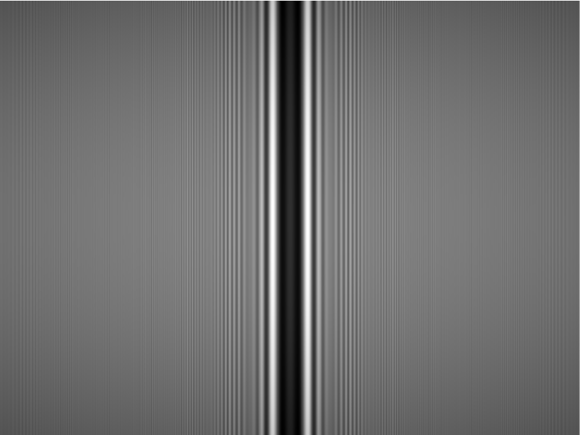
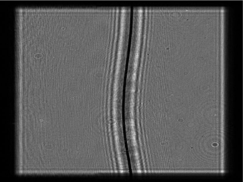
To illustrate Eq. (13), the optical set-up given on Fig. (1) is considered. We investigate the diffraction pattern obtained with an opaque fiber parallel to the pipe axis. From the Gaussian decomposition of the object function, opaque fibers, parallel to the pipe axis, can be obtained taking $R_{ell}\rightarrow 0$. The value of the opaque fiber diameter is $2b=51.8\;\textmu m$ and $a\rightarrow\infty$. The glass-made ($n_{1}=1.5$) pipe is filled with water of refractive index $n_{2}=1.33$. The beam propagates in free space over $z_{p}=325\;mm$. The dimensions $\delta$ and $z$ are fixed to 18 $mm$ and 23 $mm$ respectively.

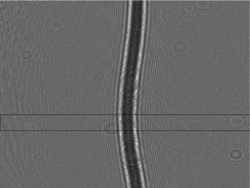
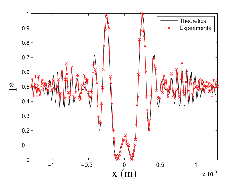
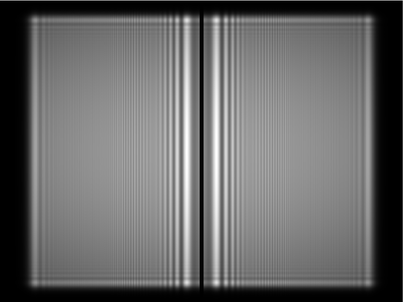
The image of Fig. (3) illustrates the intensity distribution of the diffracted field. The simulation is carried out by calculating the gray level of each pixel using Eq. (13). The size of the hologram is $768\times 576$ pixels, and pixel pitch is $11\;\textmu m$. To validate our simulation, an experiment, which consists in placing an opaque fiber in the pipe, was performed. The hologram of Fig (4) represents the intensity of the diffraction recorded with the CCD sensor using the same parameters than previously. This illustration reveals a good accordance between numerical and experimental diffraction patterns. To confirm this point, the transverse intensity profiles obtained from Fig. (3) and Fig. (4) are presented on Fig (5). Here the normalized intensity $I^{*}$ is plotted against the x-axis. The intensity profiles are calculated by cumulating the gray levels along the $\eta$-axis (direction of the fiber) over 50 rows, which are figured out by the rectangular selection on Fig. (4). The diffraction pattern of Fig. (4) was shifted by $75\;\textmu m$ along x-axis so that numerical and experimental results can be compared. This figure shows the good agreement between numerical and experimental data.

2.B Case of thin lenses

We have proposed a theoretical model allowing us to deal with propagation of a laser beam through a thick pipe. In a former study, the effect of cylindrical lenses on the diffraction pattern of a particle has been investigated in details, leading to the expression of the intensity distribution in the CCD plane [10]. Using this approach we have a great opportunity to confirm our pipe model results.

In the following developments we aim to compare our thick and cylindrical pipe model with a thin cylindrical lenses approach. The phase transformation due to a thin lens is [18, 10]:

$$\Phi\left(x_{l},y_{l}\right)=\exp\left[-i\frac{\pi}{\lambda}\left(\frac{x_{l}^{2}}{f_{x}}+\frac{y_{l}^{2}}{f_{y}}\right)\right].$$ (14)

Here $\left(x_{l},y_{l}\right)$ are the coordinates in the lens plane and $f_{x,y}$ are the focal lengths of the lens in both directions. Using Huygens-Fresnel integral [18] the intensity distribution in the sensor plane is:

$$I_{thin}\left(x,y\right)=\left|\frac{\exp\left(i\frac{2\pi}{\lambda}E_{2}\right)}{i\lambda E_{2}}\left[R_{thin}\left(x,y\right)-O_{thin}\left(x,y\right)\right]\right|^{2}.$$ (15)

Here, $R_{thin}$ and $O_{thin}$ can be expressed in a quite similar form than amplitude distributions given in Eqs. (11) and (12).

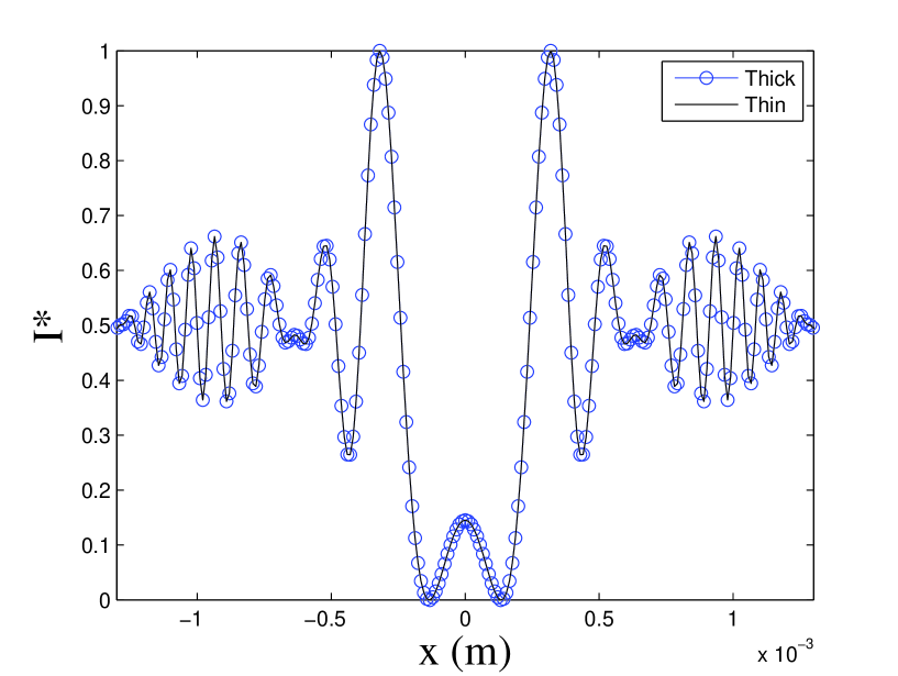
The transverse intensity distribution profile presented in Fig. (6) shows:

$$\lim_{e\rightarrow 0}I\left(x,y\right)=I_{thin}\left(x,y\right),$$ (16)

remembering that $e$ represents the glass thickness. This term is contained in matrices $M_{1}^{x,y}$ and $M_{2}^{x,y}$ (see Eqs. (38) and (39)).

For this example: $2b=51.8\;\textmu m$, $a\rightarrow\infty$, $z_{p}=325\ mm$, $n_{2}=1$, $\delta=18\ mm$ and $z=23\ mm$. The comparison with other parameter values leads to the same conclusion. As a result, we can consider that our results are consistent with those of Ref. [10] and that our model is versatile enough to deal with various pipe shapes and thickness.

In this section a numerical model allowing to treat thick optical systems has been presented. We now aim to reconstruct the image of the object by means of FRFT from the calculated intensity distribution of the diffraction pattern (Eq. (13)). In section 3, mathematical definition of the FRFT is recalled leading to the reconstruction of holograms recorded in pipe systems.

3 Fractional Fourier transformation analysis of in-line holograms

3.A Two-dimensional Fractional Fourier transformation

The FRFT is a generalization of the classical Fourier transform. This integral operator has numerous applications in signal processing [17]. Its mathematical expression is the following [27, 28, 29]: the FRFT of order $a_{x}=(2\alpha_{x})/\pi$ and $a_{y}=(2\alpha_{y})/\pi$ (for $x$ and $y$ cross section respectively), with $0\leq\left|\alpha_{x}\right|\leq\pi/2$ and $0\leq\left|\alpha_{y}\right|\leq\pi/2$, of a two dimensional function $I\left(x,y\right)$ is

$$\mathscr{F}_{\alpha_{x},\alpha_{y}}[I(x,y)](x_{a},y_{a})=\int_{\mathbb{R}^{2}}N_{\alpha_{x}}(x,x_{a})\,N_{\alpha_{y}}(y,y_{a})I(x,y)\,dx\,dy,$$ (17)

where the kernel of the fractional operator is defined by

$$N_{\alpha_{p}}(x,x_{a})=C(\alpha_{p})\exp\left(i\pi\frac{x^{2}+x_{a}^{2}}{s_{p}^{2}\tan\alpha_{p}}\right)\exp\left(-\frac{i2\pi x_{a}x}{s_{p}^{2}\sin\alpha_{p}}\right),$$ (18)

and

$$C(\alpha_{p})=\frac{\exp(-i(\frac{\pi}{4}\textrm{sign}(\sin\alpha_{p})-\frac{\alpha_{p}}{2}))}{|s_{p}^{2}\sin\alpha_{p}|^{1/2}}\,.$$ (19)

Here $p=x,y$. Generally, the parameter $s_{p}$ is considered as a normalization constant. In our case, its value is defined from the experimental set-up according to [30]: $s_{p}^{2}=N_{p}^{px}\cdot\delta_{p}^{2}$. The number of samples is $N_{p}^{px}$ in both intensity distribution $I\left(x,y\right)$ and fractional domain. $\delta_{p}$ is the sampling period along the two axes of the image. $C(\alpha_{p})$, which is a function of the fractional order, insures the energy conservation law to be valid. Discretization of the FRFT kernel is performed using an orthogonal projection method proposed by Pei et al. [31].

3.B Optimal fractional orders to refocus numerically over the object

In our case, the numerical reconstruction can be considered as a numerical refocusing over the object [32]. To do that, the quadratic phase, denoted $\varphi=\arg\left(R\overline{O}\right)$, and contained in the term $2\Re\left\{R\overline{O}\right\}$ of Eq. (13) must be evaluated. This term is composed of a linear chirp modulated by a sum of complex Gaussian functions. Information about the distance between the CCD sensor and the object is carried by the linear chirp ($B_{2_{x,y}}$) whereas information about object size is carried by the modulation ($M_{{x,y}_{eq}}$ and $N_{{x,y}_{eq}}$). The optimal reconstruction of the image consists in compensating the quadratic phase terms of the intensity distribution [10].

The quadratic phase can be determined from Eqs. (11) and (12)

$$\varphi=\frac{\pi}{\lambda}\left[\left(\frac{M_{x}-D^{x}_{2}}{B^{x}_{2}}\right)x^{2}+\left(\frac{M_{y}-D^{y}_{2}}{B^{y}_{2}}\right)y^{2}\right],$$ (20)

thus $\Re\left\{R\overline{O}\right\}$ can be written as:

$$\Re\left\{R\overline{O}\right\}=\left|R\overline{O}\right|\cos\left(i\varphi\right).$$ (21)

The quadratic phase term contained in the FRFT kernel, denoted $\varphi_{a}$, is given by

$$\varphi_{a}=\pi\left(\frac{\cot\alpha_{x}}{s_{x}^{2}}x^{2}+\frac{\cot\alpha_{y}}{s_{y}^{2}}y^{2}\right).$$ (22)

The image reconstruction is obtained by applying the FRFT to the intensity distribution of Eq. (13):

$$\mathscr{F}_{\alpha_{x},\alpha_{y}}[I(x,y)]\propto\mathscr{F}_{\alpha_{x},\alpha_{y}}[\left|R\right|^{2}+\left|O\right|^{2}]-2\mathscr{F}_{\alpha_{x},\alpha_{y}}[\left|R\overline{O}\right|\cos\varphi].$$ (23)

The terms $\left|R\right|^{2}$ and $\left|O\right|^{2}$ contain no linear chirps, thus they do not influence the optimal fractional orders of reconstruction to be determined. Only the second term is useful for image reconstruction. By noting that $2\cos\varphi=\exp\left(-i\varphi\right)+\exp\left(i\varphi\right)$, Eq. (23) becomes:

$$\mathscr{F}_{\alpha_{x},\alpha_{y}}[I(x,y)]\propto\mathscr{F}_{\alpha_{x},\alpha_{y}}[\left|R\right|^{2}+\left|O\right|^{2}]\\ -C\left(\alpha_{x}\right)C\left(\alpha_{y}\right)\int_{\mathbb{R}^{2}}\left|R\overline{O}\right|\exp\left[i\left(\varphi_{a}-\varphi\right)\right]\exp\left[-i2\pi\left(\frac{x_{a}x}{s_{x}^{2}\sin\alpha_{x}}+\frac{y_{a}y}{s_{y}^{2}\sin\alpha_{y}}\right)\right]dxdy\\ -C\left(\alpha_{x}\right)C\left(\alpha_{y}\right)\int_{\mathbb{R}^{2}}\left|R\overline{O}\right|\exp\left[i\left(\varphi_{a}+\varphi\right)\right]\exp\left[-i2\pi\left(\frac{x_{a}x}{s_{x}^{2}\sin\alpha_{x}}+\frac{y_{a}y}{s_{y}^{2}\sin\alpha_{y}}\right)\right]dxdy.$$ (24)

The best hologram reconstruction is reached when one of the quadratic phase term is brought to zero. Thus reconstruction is performed if

$$\varphi_{a}\pm\varphi=0.$$ (25)

The optimal fractional orders $\alpha_{x}^{opt}$ and $\alpha_{y}^{opt}$ are defined from Eqs. (20), (22) and (25) and take the values:

$$\alpha_{x}^{opt}=\arctan\left[\mp\frac{B^{x}_{2}\lambda}{s_{x}^{2}\left(M_{x}-D^{x}_{2}\right)}\right],\quad\alpha_{y}^{opt}=\arctan\left[\mp\frac{B^{y}_{2}\lambda}{s_{y}^{2}\left(M_{y}-D^{y}_{2}\right)}\right].$$ (26)

It should be noted that we have checked that if we consider $M_{2_{x,y}}$ to be free space propagation, leading to $B^{x,y}_{2}=z_{i}+e+z$ and $D^{x,y}_{2}=1$, the expression of the optimal fractional order of Ref.  [10] are recovered.

3.C Numerical simulations

Experimental set-up of Fig. (1) is used to perform simulations. An application of the model is illustrated on Fig. (3). Recall that we consider an opaque fiber ($R_{ell}\rightarrow 0$) $2b=51.8\mu m$ in width. The glass made pipe is filled with water ($n_{2}=1.33$). $\delta$ and $z$ are set to 18 $mm$ and 23 $mm$ respectively. $Rx_{1},Ry_{1},Ry_{2}\rightarrow\infty$ and $Rx_{2}=18\ mm$ are the first thick lens curvatures along $x$- and $y$-axis. The curvature radii of the second thick lens have the same values but opposite signs. With these parameters and owing to Eq. (26) the optimal fractional orders within this configuration are

$$a_{x}^{opt}=0.337,\quad a_{y}^{opt}=0.273.$$ (27)

The reconstruction of the fiber with FRFT can be seen on Fig. (7). As we can see on this figure, the reconstructed image is disturbed by background fringes. This effect is due to the in-line configuration and is commonly known as the twin image effect [33].

3.D Experimental results

Since now, we have presented a method to simulate holograms in thick optical systems. Reconstruction has been successfully performed thanks to FRFT. In order to validate theoretical developments and simulations, a glass pipe with curvatures $Rx_{1},Ry_{1},Ry_{2}\rightarrow\infty$ and $Rx_{2}=18\ mm$ has been used for the experiments. Curvatures on the other side of the pipe are deduced from $Rx_{1},Ry_{1},Rx_{2},Ry_{2}$ by taking negative values.

The image of Fig. (4) represents the intensity of the diffraction pattern recorded with a $768\times 576\ px^{2}$ CCD sensor with $11\ \mu m$ pitch. The object is a $2b=51.8\mu m$ opaque fiber, $\delta$ and $z$ are approximately and respectively equal to $18\ mm$ and $23\ mm$. Theoretical orders associated with this experiment are given by Eq. (27). To perform FRFT on this experimental image, FRFT orders have been adjusted to obtain the best image of the fiber i. e the best contrast between the reconstructed fiber and the background. Thus doing, the accuracy on the fractional order is approximately $10^{-2}$. Reconstruction is presented on Fig. (8), estimated optimal fractional orders are $a_{x}=0.33$ and $a_{y}=0.27$. These values are very close to the theoretical ones.

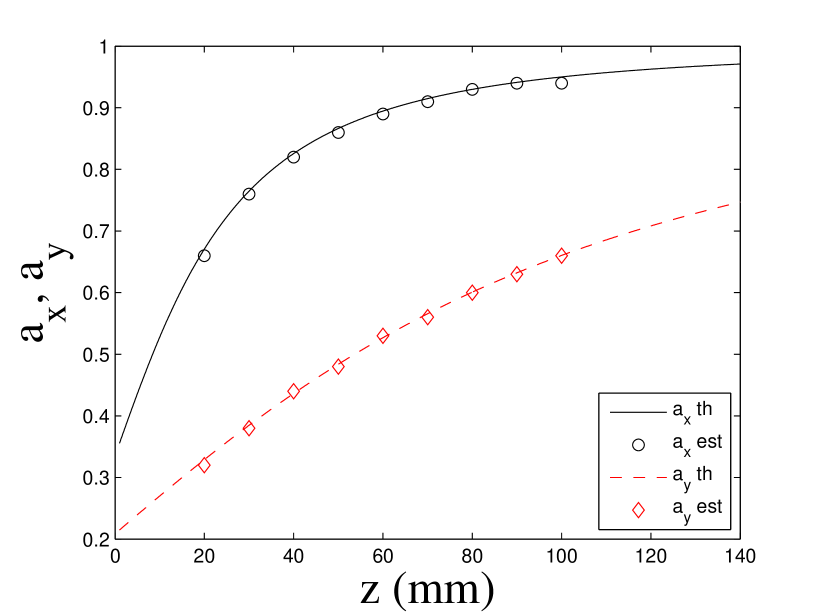
This good accordance is confirmed by the curves of Fig. (9). Here theoretical values of $a_{x}^{opt}$ (solid line) and $a_{y}^{opt}$ (dashed line) are plotted versus the distance between the pipe and the CCD sensor. Theoretical values corresponds to an air filled glass pipe, $\delta$ is fixed to $10\ mm$ and $z$ varies from 0 to $140\ mm$. Note that, when $z=0$, $a_{x,y}\neq 0$, this is due to the fact that, in this case, $z$ represents the distance between the pipe and the CCD sensor instead of the distance between the object and the CCD sensor which is considered in [10]. Experiments performed with this configuration allow us to plot estimated values of $a_{x}^{opt}$ (circles) and $a_{y}^{opt}$ (diamonds) on the same graph. As shown by Fig. (9), estimated and theoretical values are closely linked. Theoretical representation hereby presented is therefore well adapted to these optical systems.

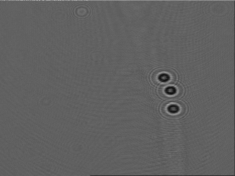
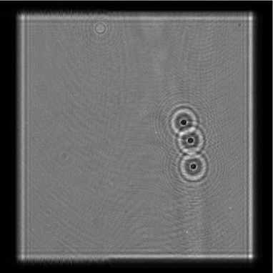
Until then, we have performed reconstruction with objects for which position is well known. We now apply our formalism to reconstruct hologram of latex beads. The intensity distribution of the diffracted field is represented on Fig. (10). Here, $100\;\textmu m$ in diameter latex beads are used, $z_{p}=325\;mm$ (i.e. propagation distance between the source and the pipe) and $z=23\;mm$ (i.e. distance between the pipe and the CCD sensor). This study gives us the opportunity to compare reconstruction using our novel approach with reconstruction using a thin lens approach. As far as every parameter of the experimental set-up is known, excepting $\delta$, the reconstruction process is the following: for $\delta\in\left[0,36\;mm\right]$ we calculate the optimal FRFT orders using Eq. (26). Doing so, we are able to refocus on the particles which are in the pipe.

In Fig. (6), it is shown that when the pipe thickness $e$ is close to zero, the two approaches are equivalent. Thus, to reconstruct the hologram of Fig. (10) with the thin lens approach, we only need to use the orders given in Eq. (26) with $e=0$.

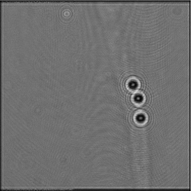
Comparison between the two reconstruction methods can be made with Fig. (11). Here, the reconstruction is realized with the same value of $\delta$ in both cases. We can notice that refocusing on the particle is impossible with the thin lens approach, whereas our thick lens approach allows a good reconstruction of the image of particles.

Therefore, the thick lens formalism is well adapted to pipe flow studies: as we are able to refocus on particles in a pipe, metrologies of particles diameter is possible.

4 Conclusion

In this paper, an analytical expression of the scalar diffraction, under Fresnel approximations, in thick optical systems such as pipes is derived. As such optical systems reveals astigmatism, FRFT is a reliable tool to perform hologram reconstruction. Optimal fractional orders have been calculated leading to a satisfactory reconstruction of either numerical or experimental images. Numerical experiments have been performed showing a good agreement with experimental results. Comparison between thin lens and thick lens approaches has been performed showing that the thin lens formalism is not well adapted to the study of pipe flows.

Appendix A Appendix A : Transfer matrices of the optical system

Each part of an optical system can be represented by a matrix. Using this principle, we can build a set of matrices corresponding to our experiments (Fig. (1)). After the beam shaping step, the beam propagates in free space over a distance $z_{p}$. The associated $M_{z_{p}}$ matrix is:

$$M_{z_{p}}=\left(\begin{array}[]{cc}1&z_{p}\\ 0&1\\ \end{array}\right).$$ (28)

Then the beam is refracted at the interface between free space and glass ($n_{1}=1.5$). The curvatures along both directions are $Rx_{1}$ and $Ry_{1}$. $M_{Rx_{1}},\ M_{Ry_{1}}$ matrices along $x$ and $y$ axis are:

$$M_{Rx_{1}}=\left(\begin{array}[]{cc}1&0\\ \frac{n_{0}-n_{1}}{Rx_{1}}&1\\ \end{array}\right),\quad M_{R1_{y}}=\left(\begin{array}[]{cc}1&0\\ \frac{n_{0}-n_{1}}{Ry_{1}}&1\\ \end{array}\right).$$ (29)

After refraction, the beam propagates in glass ($n_{1}$=1.5). For this step:

$$M_{e}=\left(\begin{array}[]{cc}1&\frac{e}{n_{1}}\\ 0&1\\ \end{array}\right),$$ (30)

Next step is the refraction of the beam at the interface between glass and the medium inside the pipe (refractive index $n_{2}$). Curvature are given by $Rx_{2}$ and $Ry_{2}$ in $x$ and $y$ direction.

$$M_{Rx_{2}}=\left(\begin{array}[]{cc}1&0\\ \frac{n_{1}-n_{2}}{Rx_{2}}&1\\ \end{array}\right),\quad M_{Ry_{2}}=\left(\begin{array}[]{cc}1&0\\ \frac{n_{1}-n_{2}}{Ry_{2}}&1\\ \end{array}\right),$$ (31)

We are now in the pipe. To reach the object, we have to propagate over $\delta$.

$$M_{\delta}=\left(\begin{array}[]{cc}1&\frac{\delta}{n_{2}}\\ 0&1\\ \end{array}\right).$$ (32)

Doing the same over $z_{i}$ permit to reach the output of the pipe:

$$M_{z_{i}}=\left(\begin{array}[]{cc}1&\frac{z_{i}}{n_{2}}\\ 0&1\\ \end{array}\right).$$ (33)

After a refraction at the interface (curvature $Rx_{3}$ and $Ry_{3}$) between the medium with refractive index $n_{2}$ and glass:

$$M_{Rx_{3}}=\left(\begin{array}[]{cc}1&0\\ \frac{n_{2}-n_{1}}{Rx_{3}}&1\\ \end{array}\right),\quad M_{Ry_{3}}=\left(\begin{array}[]{cc}1&0\\ \frac{n_{2}-n_{1}}{Ry_{3}}&1\\ \end{array}\right),$$ (34)

a propagation in glass ($n_{1}$=1.5)

$$M_{e}=\left(\begin{array}[]{cc}1&\frac{e}{n_{1}}\\ 0&1\\ \end{array}\right),$$ (35)

a refraction at the interface (curvature $Rx_{4}$ and $Ry_{4}$) between glass ($n_{1}$=1.5) and free space:

$$M_{Rx_{4}}=\left(\begin{array}[]{cc}1&0\\ \frac{n_{1}-n_{0}}{Rx_{4}}&1\\ \end{array}\right),\quad M_{Ry_{4}}=\left(\begin{array}[]{cc}1&0\\ \frac{n_{1}-n_{0}}{Ry_{4}}&1\\ \end{array}\right),$$ (36)

and free space propagation over $z$:

$$M_{z}=\left(\begin{array}[]{cc}1&z\\ 0&1\\ \end{array}\right),$$ (37)

the whole ABCD system is described.

Appendix B Appendix B : Amplitude distributions $R\left(x,y\right)$ and $O\left(x,y\right)$

In Appendix A each part of our optical system has been represented with transfer matrices. Using this formalism allows us, under paraxial conditions, to deal with propagation of a Gaussian point source through the pipe.

Intensity distribution of the diffraction pattern in the CCD sensor plane is determined by considering two matrix systems: $M_{1}^{x,y}$ and $M_{2}^{x,y}$.

$M_{1}^{x,y}$ is composed of three steps : propagation in free space over $z_{p}$, propagation through the first thick lens, propagation in a medium of refractive index $n_{2}$ over $\delta$. It is characterized by two transfer matrices:

$$M_{1}^{x,y}=M_{\delta}\times M_{L_{1}}^{x,y}\times M_{z_{p}}=\left(\begin{array}[]{cc}A^{x,y}_{1}&B^{x,y}_{1}\\ C^{x,y}_{1}&D^{x,y}_{1}\\ \end{array}\right).$$ (38)

$M_{2}^{x,y}$ is also composed of three steps : propagation in a medium of refractive index $n_{2}$ over $z_{i}$, propagation through the second thick lens, propagation in free space over $\delta$. Transfer matrices for this system are:

$$M_{2}^{x,y}=M_{z}\times M_{L_{2}}^{x,y}\times M_{z_{i}}=\left(\begin{array}[]{cc}A^{x,y}_{2}&B^{x,y}_{2}\\ C^{x,y}_{2}&D^{x,y}_{2}\\ \end{array}\right).$$ (39)

Thanks to Eqs. (29), (30), (31) one can build the transfer matrices of the first thick lens:

$$M_{L_{1}}^{x}=M_{Rx_{2}}\times M_{e}\times M_{Rx_{1}},\quad M_{L_{1}}^{y}=M_{Ry_{2}}\times M_{e}\times M_{Ry_{1}}.$$ (40)

By using the same method for the second lens, we obtain:

$$M_{L_{2}}^{x}=M_{Rx_{4}}\times M_{e}\times M_{Rx_{3}},\quad M_{L_{2}}^{y}=M_{Ry_{4}}\times M_{e}\times M_{Ry_{3}}.$$ (41)

B.A Propagation through $M_{1}^{x,y}$

After analytical developments of Eq. (2), the complex amplitude distribution in the object plane is:

$$G_{1}\left(\xi,\eta\right)=\frac{\exp\left(i\frac{2\pi}{\lambda}E_{1}\right)}{i\lambda\sqrt{B^{x}_{1}B^{y}_{1}}}K_{1}^{x}K_{1}^{y}\exp\left[-\left(\frac{\xi^{2}}{\omega_{1_{x}}^{2}}+\frac{\eta^{2}}{\omega_{1_{y}}^{2}}\right)\right]\exp\left[-i\frac{\pi}{\lambda}\left(\frac{\xi^{2}}{R_{1_{x}}}+\frac{\eta^{2}}{R_{1_{y}}}\right)\right],$$ (42)

with $K_{1}^{x,y}$ given by:

$$K_{1}^{x,y}=\left(\frac{\pi\omega^{2}}{1-iA^{x,y}_{1}\frac{\pi\omega^{2}}{\lambda B^{x,y}_{1}}}\right)^{1/2},$$ (43)

$\omega_{1_{x,y}}$ and $R_{1_{x,y}}$ are respectively the beam radii and the wavefront curvature in the particle plane. Their mathematical expressions are:

$$\omega_{1_{x,y}}=\left(\frac{\lambda B^{x,y}_{1}}{\pi\omega}\right)\left[1+\left(A^{x,y}_{1}\frac{\pi\omega^{2}}{\lambda B^{x,y}_{1}}\right)^{2}\right]^{1/2},\quad R_{1_{x,y}}=-\frac{B^{x,y}_{1}}{D^{x,y}_{1}-\frac{A^{x,y}_{1}\left(\frac{\pi\omega^{2}}{\lambda B^{x,y}_{1}}\right)^{2}}{1+\left(A^{x,y}_{1}\frac{\pi\omega^{2}}{\lambda B^{x,y}_{1}}\right)^{2}}}.$$ (44)

B.B Propagation through $M_{2}^{x,y}$

Propagation to the CCD sensor plane is calculated thanks to the generalized Huygens-Fresnel integral (see Eq. (3)).

B.B.1 Amplitude distribution $R\left(x,y\right)$

$R$ is associated with the reference wave. After analytical developments of Eq. (9), the amplitude distribution $R$ is:

$$R\left(x,y\right)=\frac{\exp\left(i\frac{2\pi}{\lambda}E_{1}\right)}{i\lambda\sqrt{B^{x}_{1}B^{y}_{1}}}K_{1}^{x}K_{1}^{y}K_{2}^{x}K_{2}^{y}\\ \times\exp\left[-\frac{\pi}{\lambda}\left(\frac{N_{x}}{B^{x}_{2}}x^{2}+\frac{N_{y}}{B^{y}_{2}}y^{2}\right)\right]\exp\left[i\frac{\pi}{\lambda}\left(\frac{M_{x}}{B^{x}_{2}}x^{2}+\frac{M_{y}}{B^{y}_{2}}y^{2}\right)\right],$$ (45)

where,

$$M_{x,y}=D^{x,y}_{2}+\frac{\left(\frac{\pi\omega_{1_{x,y}}^{2}}{\lambda B^{x,y}_{2}}\right)^{2}\left(\frac{B^{x,y}_{2}}{R_{1_{x,y}}}-A^{x,y}_{2}\right)}{1+\left(\frac{\pi\omega_{1_{x,y}}^{2}}{\lambda B^{x,y}_{2}}\right)^{2}\left(\frac{B^{x,y}_{2}}{R_{1_{x,y}}}-A^{x,y}_{2}\right)^{2}},\quad N_{x,y}=\frac{\frac{\pi\omega_{1_{x,y}}^{2}}{\lambda B^{x,y}_{2}}}{1+\left(\frac{\pi\omega_{1_{x,y}}^{2}}{\lambda B^{x,y}_{2}}\right)^{2}\left(\frac{B^{x,y}_{2}}{R_{1_{x,y}}}-A^{x,y}_{2}\right)^{2}},$$ (46)

and

$$K_{2}^{x,y}=\left[\frac{\pi\omega_{1_{x,y}}^{2}}{1+i\frac{\pi\omega_{1_{x,y}}^{2}}{\lambda B^{x,y}_{2}}\left(\frac{B^{x,y}_{2}}{R_{1_{x,y}}}-A^{x,y}_{2}\right)}\right]^{1/2}.$$ (47)

B.B.2 Amplitude distribution $O\left(x,y\right)$

$O$ is the amplitude of the diffracted wave. We define $\omega_{{1_{x,y}}_{eq}}$ and $R_{{1_{x,y}}_{eq}}$

$$\frac{1}{\omega_{{1_{x}}_{eq}}^{2}}=\frac{1}{\omega_{1_{x}}^{2}}+\frac{\Re\{B_{k}\}}{b^{2}},\quad\frac{1}{\omega_{{1_{y}}_{eq}}^{2}}=\frac{1}{\omega_{1_{y}}^{2}}+R_{ell}^{2}\frac{\Re\{B_{k}\}}{b^{2}},$$ (48)

and

$$\frac{1}{R_{{1_{x}}_{eq}}}=\frac{1}{R_{1_{x}}}+\frac{\Im\{B_{k}\}\lambda}{\pi b^{2}},\quad\frac{1}{R_{1{{}_{y}}_{eq}}}=\frac{1}{R_{1_{y}}}+R_{ell}^{2}\frac{\Im\{B_{k}\}\lambda}{\pi b^{2}},$$ (49)

to simplify notations. It should be noted that $\Re$ and $\Im$ stand for real and imaginary part respectively. Thus $O$ becomes:

$$O\left(x,y\right)=\frac{\exp\left(i\frac{2\pi}{\lambda}E_{1}\right)}{i\lambda\sqrt{B^{x}_{1}B^{y}_{1}}}K_{1}^{x}K_{1}^{y}\exp\left[i\frac{\pi}{\lambda}\left(\frac{D^{x}_{2}}{B^{x}_{2}}x^{2}+\frac{D^{y}_{2}}{B^{y}_{2}}y^{2}\right)\right]\sum_{k=1}^{N}A_{k}K_{2}^{{x}_{eq}}K_{2}^{{y}_{eq}}\\ \times\exp\left[-\frac{\pi}{\lambda}\left(\frac{N_{x_{eq}}}{B^{x}_{2}}x^{2}+\frac{N_{y_{eq}}}{B^{y}_{2}}y^{2}\right)\right]\exp\left[i\frac{\pi}{\lambda}\left(\frac{M_{x_{eq}}}{B^{x}_{2}}x^{2}+\frac{M_{y_{eq}}}{B^{y}_{2}}y^{2}\right)\right],$$ (50)

with

$$M_{{x,y}_{eq}}=\frac{\left(\frac{\pi\omega_{{1_{x,y}}_{eq}}^{2}}{\lambda B^{x,y}_{2}}\right)^{2}\left(\frac{B^{x,y}_{2}}{R_{{1_{x,y}}_{eq}}}-A^{x,y}_{2}\right)}{1+\left(\frac{\pi\omega_{{1_{x,y}}_{eq}}^{2}}{\lambda B^{x,y}_{2}}\right)^{2}\left(\frac{B^{x,y}_{2}}{R_{{1_{x,y}}_{eq}}}-A^{x,y}_{2}\right)^{2}},\\ N_{{x,y}_{eq}}=\frac{\frac{\pi\omega_{{1_{x,y}}_{eq}}^{2}}{\lambda B^{x,y}_{2}}}{1+\left(\frac{\pi\omega_{{1_{x,y}}_{eq}}^{2}}{\lambda B^{x,y}_{2}}\right)^{2}\left(\frac{B^{x,y}_{2}}{R_{{1_{x,y}}_{eq}}}-A^{x,y}_{2}\right)^{2}},$$ (51)

and

$$K_{2}^{{{x,y}_{eq}}}=\left[\frac{\pi\omega_{1_{{x,y}_{eq}}}^{2}}{1+i\frac{\pi\omega_{1_{{x,y}_{eq}}}^{2}}{\lambda B^{x,y}_{2}}\left(\frac{B^{x,y}_{2}}{R_{1_{{x,y}_{eq}}}}-A^{x,y}_{2}\right)}\right]^{1/2}.$$ (52)

Fig. 1: a) Schematic representation of the optical set-up (not to scale). Definition of the numerical and experimental parameters. b) Close-up of the pipe used in simulations and experiments

Fig. 2: Schematic representation of the object.

Fig. 3: Simulation of the diffraction pattern of a 51.8 $\mu m$ opaque fiber, parallel to the axis of a glass pipe, $n_{2}=1.33$, $\lambda=632.8nm$, $z=23mm$, $\delta=18mm$.

Fig. 4: Experimental diffraction pattern of a 51.8 $\mu m$ opaque fiber, parallel to the axis of a glass pipe, $n_{2}=1.33$, $\lambda=632.8nm$, $z=23mm$, $\delta=18mm$.

Fig. 5: Comparison between simulated and experimental intensity distributions

Fig. 6: Normalized intensity distribution recorded by the CCD: comparison between thin lens and thick lens models, with $e=0\;mm$. Simulation parameters are : $2b=51.8\;\textmu m$, $a\rightarrow\infty$, $z_{p}=325\ mm$, $n_{2}=1$, $\delta=18\ mm$ and $z=23\ mm$

Fig. 7: Reconstruction of the fiber image from the diffraction pattern of Fig. (3) by FRFT with $a_{x}^{opt}=0.337$ and $a_{y}^{opt}=0.273$.

Fig. 8: Reconstruction of the fiber image from the diffraction pattern of Fig. (4) by FRFT with $a_{x}^{opt}=0.33$ and $a_{y}^{opt}=0.27$.

Fig. 9: Comparison between theoretical fractional orders and optimal fractional orders estimated from the experimental holograms.

Fig. 10: Experimental diffraction pattern of $100\textmu m$ latex beads. $z_{p}=325\ mm$, $z=23\ mm$.

Fig. 11: Reconstruction of the latex beads image. (a) Reconstruction with thin lens parameters. (b) Reconstruction using thick lens approach.

References

- [1] G. Pan, H. Meng, ”Digital holography of particle fields: reconstruction by use of complex amplitude,” Appl. Opt. 42, 827-833 (2003).
- [2] M. Malek, D. Allano, S. Coëtmellec, C. Özkul, D. Lebrun, ”Digital in-line holography for three-dimensional-two-components particle tracking velocimetry,” Meas. Sci. Technol. 15, 699-705 (2004).
- [3] E. Malkiel, J. Sheng, J. Katz, J. Strickler, ”The three-dimensional flow field generated by a feeding calanoid copepod measured using digital holography,” J. Exp. Bio. 206, 3657-3666 (2003).
- [4] J. Garcia-Sucerquia, W. Xu, S. Jericho, P. Klages, M. Jericho, H. Kreuzer, ”Digital in-line holographic microscopy,” Appl. Opt. 45, 836-850 (2006).
- [5] C.S. Vikram, ”Particle field holography,” Cambridge Studies in Modern Optics, (1992).
- [6] S. De Nicola, P. Ferraro, A. Finizio, G. Pierattini, ”Correct-image reconstruction in the presence of severe anamorphism by means of digital holography,” Opt. Lett. 26, 974-976 (2001).
- [7] S. Grilli, P. Ferraro, S. De Nicola, A. Finizio, G. Pierattini, R. Meucci, ”Whole optical wavefields reconstruction by Digital Holography,” Opt. Express 9, 294-302 (2001).
- [8] S. De Nicola, P. Ferraro, A. Finizio, G. Pierattini, ”Wave front reconstruction of Fresnel off-axis holograms with compensation of aberrations by means of phase-shifting digital holography,” Opt. Laser Eng. 37, 331-340 (2002).
- [9] J.S. Crane, P. Dunn, B.J. Thompson, J.Z. Knapp, J. Zeiss, ”Far-field holography of ampule contaminants,” Appl. Opt. 21, 2548-2553 (1982).
- [10] F. Nicolas, S. Coëtmellec, M. Brunel, D. Allano, D. Lebrun, and A. J. Janssen, ”Application of the fractional Fourier transformation to digital holography recorded by an elliptical, astigmatic Gaussian beam,” J. Opt. Soc. Am. A 22, 2569-2577 (2005).
- [11] L. Onural, P. Scott, ”Digital decoding of in-line holograms,” Opt. Eng. 26, 1124-1132 (1987).
- [12] L. Onural, ”Diffraction from a wavelet point of view,” Opt. Lett. 18, 846-848 (1993).
- [13] F. Nicolas, S. Coëtmellec, M. Brunel and D. Lebrun, ”Digital in-line holography with a sub-picosecond laser beam,” Optics Communications 268, 27-33 (2006).
- [14] C. Palma, V. Bagini, ”Extension of the Fresnel transform to ABCD systems,” J. Opt. Soc. Am. A 14, 1774-1779 (1997).
- [15] A.J. Lambert, D. Fraser, ”Linear systems approach to simulation of optical diffraction,” Appl. Opt. 37, 7933-7939 (1998).
- [16] H.T. Yura, S.G. Hanson, ”Optical beam wave propagation through complex optical systems,” J. Opt. Soc. Am. A 4, 1931-1948 (1987).
- [17] H.M. Ozaktas, Z. Zalevsky, M.A. Kutay, The Fractional Fourier Transform: with Applications in Optics and Signal Processing, Wiley, (2001).
- [18] J.W. Goodman, Introduction to Fourier Optics, Roberts and Company, third edition, (2005).
- [19] A.E. Siegman, Lasers, University Science Books, Sausalito, California, (1986).
- [20] J.J. Wen, M. Breazeale, ”Gaussian beam functions as a base function set for acoustical field calculations,” Proc IEEE Ultrasonics Symposium, 1137-1140 (1987).
- [21] J.J. Wen, M. Breazeale, ”A diffraction beam expressed as the superposition of Gaussian beams,” J. Acoust. Soc. Am. 83, 1752-1756 (1988).
- [22] C. Zheng, D. Zhao, X. Du, ”Analytical expression of elliptical Gaussian beams through nonsymmetric systems with an elliptical aperture,” Optik 117, 296-298 (2005).
- [23] X. Du, D. Zhao, ”Propagation of decentered elliptical Gaussian beams in apertured and nonsymmetrical optical systems,” J. Opt. Soc. Am. A 23, 625-631 (2006).
- [24] X. Du, D. Zhao, ”Propagation of elliptical Gaussian beams in apertured and misaligned optical systems,” J. Opt. Soc. Am. A 23, 1946-1950 (2006).
- [25] X. Du, D. Zhao, ”Propagation of elliptical Gaussian beams modulated by an elliptical annular aperture,” J. Opt. Soc. Am. A 24, 444-450 (2007).
- [26] F. Slimani, G. Grehan, G. Gouesbet, D. Allano, ”Near-field Lorenz-Mie theory and its application to microholography,” Appl. Opt. 23, 4140-4148 (1984).
- [27] A.C. McBride, F.H. Kerr, ”On Namias’s fractional Fourier transforms,” IMA J. Appl. Math 39, 159-175 (1987).
- [28] V. Namias, ”The fractional order Fourier transform and its application to quantum mechanics,” J. Inst. Maths Its Applics 25, 241-265 (1980).
- [29] A.W. Lohmann, ”Image rotation, Wigner rotation, and the fractional Fourier transform,” J. Opt. Soc. Am. A 10, 2180-2186 (1993).
- [30] D. Mas, J. Pérez, C. Hernández, C. Vázquez, J. J. Miret and C. Illueca, ”Fast numerical calculation of Fresnel patterns in convergent systems,” Optics Communications 227, 245-258 (2003).
- [31] S-C Pei, M-H Yeh, C-C Tseng, ”Discrete Fractional Fourier Transform Based on Orthogonal Projections,” IEEE Trans. Signal Processing 47, 1335-1348 (1999).
- [32] N. Verrier, S. Coëtmellec, M. Brunel, D. Lebrun and A.J.E.M. Janssen, ”Digital in-line holography with an elliptical, astigmatic Gaussian beam: wide-angle reconstruction,” J. Opt. Soc. Am. A, 25, 1459-1466 (2008).
- [33] D. Gabor, ”Microscopy by reconstructed wave-fronts,” Proc. Roy. Soc. A. 197, 454-487 (1949)