Online Myopic Network Covering

Abstract

Efficient marketing or awareness-raising campaigns seek to recruit $n$ influential individuals – where $n$ is the campaign budget – that are able to cover a large target audience through their social connections. So far most of the related literature on maximizing this network cover assumes that the social network topology is known. Even in such a case the optimal solution is NP-hard. In practice, however, the network topology is generally unknown and needs to be discovered on-the-fly. In this work we consider an unknown topology where recruited individuals disclose their social connections (a feature known as one-hop lookahead). The goal of this work is to provide an efficient greedy online algorithm that recruits individuals as to maximize the size of target audience covered by the campaign.

We propose a new greedy online algorithm, Maximum Expected $d$-Excess Degree (MEED), and provide, to the best of our knowledge, the first detailed theoretical analysis of the cover size of a variety of well known network sampling algorithms on finite networks. Our proposed algorithm greedily maximizes the expected size of the cover. For a class of random power law networks we show that MEED simplifies into a straightforward procedure, which we denote MOD (Maximum Observed Degree). We substantiate our analytical results with extensive simulations and show that MOD significantly outperforms all analyzed myopic algorithms. We note that performance may be further improved if the node degree distribution is known or can be estimated online during the campaign.

1 Introduction

This paper addresses the need to efficiently select $n$ individuals in a network such that they cover, through their neighbors, the largest possible fraction of the network. Online social networks have generated much attention as a breeding ground for new forms of social studies, social mobilization, and online campaigns. Recruiting individuals from a population – for instance, recruiting volunteers to get their friends to vote in an election – is no easy task. The recruitment of each individual comes at a cost in time, money, and social capital; and the total budget is often small with respect to the total population. Moreover, recruitment is frequently targeted towards a subpopulation – say, individuals that will likely vote for a given candidate – that may be a relatively small fraction of the whole population. Most works on network cover, e.g. [MaiyaKDD, Guha1998, Garey1990], either consider the social network topology to be known in advance or assume the capability of a two-hop lookahead (where the identity of all nodes within a two-hop neighborhood of a recruited node are known), which is often not the case in the wild.

In this work we look at the cover problem when the network topology is unknown. Following previous literature, we assume that any individual in the network can be recruited – but in our case recruitments mostly happen through friends recruiting friends. This link-tracing technique has been long used by social scientists to sample hard-to-reach subpopulations [Krista, RDS, Salganik]. The homophily often present in social networks – the tendency for similar individuals to be friends [MSC] – enables the likely effective recruitment of individuals that are either in the target subpopulation or know many unrecruited individuals in the target subpopulation. This is achieved simply by asking each recruited individual to refer other target individuals.

The recent 2012 U.S. presidential election presents a real-life example of an application of link-tracing recruitments to maximize the network cover of a target subpopulation. A candidate’s Facebook app asked its subscribers to send get-out-to-vote reminders to their like-minded friends in swing states [FB]. Thus, the effectiveness of a subscriber is measured by the amount of its friends that live in swing states. Moreover, these messages also raised awareness of the app itself, allowing it to spread through the target subpopulation of interest (see also Bond et al. [VoteNature] for a description of a get-out-to-vote Facebook app experiment in the 2010 U.S. elections).

Problem Formulation

We formulate the target subpopulation cover problem as a maximum connected cover (MCC) problem on an unknown connected graph $G=(V,E)$ (we also refer to $G$ as a network), where $V$ is the set of target individuals and $E$ the set of individuals’ mutual connections. We assume all graph parameters are unknown. Our analysis can be easily extended to a disconnected network by considering each connected component separately.

Our main goal is to design efficient online greedy algorithms to solve the following problem on $G$: let $n$ be a given campaign budget; we want to determine a group of $n$ individuals to be recruited in order to maximize the size of the covered subset, i.e. of the set including the recruited nodes and their neighbors. Our only initially available information is a single node sampled from the population. Later we can acquire the neighborhood of any recruited node. It follows that the recruited nodes form a connected subgraph.

More formally, let $\mathcal{B}(t)$ be the set of $t$ known target individuals after $t$ recruitments (also denoted the $t$-th step). Let $\mathcal{B}(0)$ be the set containing the initially known individual Let $\mathcal{N}(\mathcal{B}(t))$ be a function that returns the set of unrecruited neighbors of $\mathcal{B}(t)\subseteq V$; Fig. 1 illustrates $\mathcal{B}(t)$ and $\mathcal{N}(\mathcal{B}(t))$. The online algorithm proceeds as follows: at step $t$, $0<t\leq n$, the algorithm recruits node $v\in\mathcal{N}(\mathcal{B}(t-1))$ and performs the update $\mathcal{B}(t)=\mathcal{B}(t-1)\cup\{v\}$. The ability to obtaining the identities of the neighbors of recruited nodes, $\mathcal{N}(\mathcal{B}(t))$, $\forall t$, is known as one-hop lookahead in the graph sampling literature [Adamic, MST06]. The objective of the online algorithm is to try to maximize the size of the network cover set $\mkern 1.5mu\overline{\mkern-1.5mu\mathcal{W}\mkern-1.5mu}\mkern 1.5mu(t)=\mathcal{B}(t)\cup\mathcal{N}(\mathcal{B}(t))$, for $t=1,\ldots,n$, without having a priori access to topology information. We refer to the problem of online covering an unknown network in the presence of one-hop lookahead as the online myopic network covering problem.

Contributions

We make the following contributions:

(1) We thoroughly evaluate – analytically and through extensive simulations on social network datasets – the performance of several known network sampling algorithms. (1.1) We investigate the cover sizes of Breadth-First Search (BFS) and Depth-First Search (DFS). We observe a consistent large variance in the cover sizes found by BFS and that BFS tends to underperform in comparison to a greedy oracle scheme that recruits at every step the node with the largest number of uncovered neighbors. We partially blame network homophily for the lack of performance from BFS. DFS, which at first sight should improve upon BFS in circumventing the above homophily problem, performs even worse. Using random networks, we show why DFS finds a small cover after $t\ll N$ recruited nodes. (1.2) A Random Walk (RW), more precisely RW without replacement (RWnr), where nodes revisited by the walker are not counted towards the recruitment budget, is shown to consistently outperform (sometimes significantly) BFS in our simulations. (1.3) We propose a new online algorithm inspired by the Susceptible-Infected (SI) epidemic model but observe that RWnr is consistently more efficient than SI.

(2) Our work is, to the best of our knowledge, the first to provide an analytical characterization of the sizes of $\mkern 1.5mu\overline{\mkern-1.5mu\mathcal{W}\mkern-1.5mu}\mkern 1.5mu(t)$ (the cover) as a function of $t$ (recruited nodes), for RWnr and the SI epidemic algorithms on finite networks. As recently acknowledged in [FPS12], this was a challenging open problem. Moreover, we establish an interesting connection between cover through RWs and the coupon subset collection problem. We validate our theoretical results through simulations.

(3) We propose a new online algorithm (MEED, Maximum Expected $d$-Excess Degree) that greedily maximizes the expected size of the cover. For a broad class of power law networks, MEED simplifies into a straight forward heuristic, which we denote Maximum Observed Degree (MOD). We substantiate our analytical results with simulations. Extensive simulations on a variety of social network datasets show that MOD consistently outperforms (sometimes significantly) all other analyzed algorithms. Performance can be further improved if the node degree distribution is known or can be estimated online during the campaign.

Outline

The reminder of this work is organized as follows. Sec. 2 presents the notation and background used throughout this work. Sec. 3 discusses optimal solutions and approximations in connection to the connected minimum dominating set. Sec. 4 presents the datasets used in this work and our simulation setup. Sec. 5 provides an analysis of the effectiveness of Breadth-First-Search (BFS) and Depth-First-Search (DFS). Sec. 6 provides a deep analysis of the effectiveness of two types of random walks and compare them to BFS. Sec. LABEL:sec:SI proposes a sampling algorithm inspired by Susceptible-Infected (SI) epidemic models. We also provide an analytical solution describing the cover size of SI as a function of $t$. An important feature of our analysis is our ability to model finite graphs, which is key to understanding the effectiveness of large campaigns in respect to the size of the target population. Sec. LABEL:sec:excess proposes MEED and MOD as a simple approximation of MEED. Sec. LABEL:sec:excess also provides theoretical and simulation results, the latter comparing MOD against the other algorithms. And, finally, Sec. LABEL:sec:related summarizes our contributions and reviews the related work.

2 Notation & Background

We consider an unknown connected network $G=(V,E)$ with $N=|V|$ nodes, $M=|E|$ edges, and degree distribution $\{p_{k}\}_{k=1,\dots N-1}$. We assume all graph parameters are unknown to us. Denote $\mathcal{N}_{a}(v)$ the set of neighbors of node $v\in V$, irrespective of their recruitment status, and $k_{v}=|\mathcal{N}_{a}(v)|$ is the degree of $v$. For each step $t=1,\ldots,n$, where $n\in\{1,\ldots,N-1\}$ is the campaign budget, we classify the nodes in $V$ into three disjoint sets. The set $\mathcal{B}(t)$ denotes the recruited nodes at step $t$; these are the black nodes in Fig. 1. Unrecruited neighbors of recruited nodes are denoted observed nodes and form the set $\mathcal{N}(\mathcal{B}(t))=\cup_{v\in\mathcal{B}(t)}\mathcal{N}_{a}(v)-\mathcal{B}(t)$ (gray nodes in Fig. 1). We say a node $v\in V$ is covered at step $t$ if $v\in\mkern 1.5mu\overline{\mkern-1.5mu\mathcal{W}\mkern-1.5mu}\mkern 1.5mu(t)$, where $\mathcal{W}(t)=V-\mathcal{B}(t)\cup\mathcal{N}(\mathcal{B}(t))$ is the set of all uncovered nodes (white nodes in Fig. 1) and $\mkern 1.5mu\overline{\mkern-1.5mu\mathcal{W}\mkern-1.5mu}\mkern 1.5mu(t)=V-\mathcal{W}(t)$ its complement. Note that at time $t$ we are unaware of the existence of nodes in $\mathcal{W}(t)$.

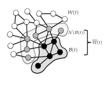
Figure 1: Network sampling evolving sets.

The sizes of the three sets $\mathcal{B}(t)$, $\mathcal{N}(\mathcal{B}(t))$, and $\mathcal{W}(t)$ are denoted $B(t)$, $\textsf{N}(\mathcal{B}(t))$ and $W(t)$, respectively. Clearly $B(t)+\textsf{N}(\mathcal{B}(t))+W(t)=N$ at any step $1\leq t\leq n$. Finally, for the sake of simplicity, we allow a slight abuse of notation, denoting by $\langle.\rangle$ both the empirical mean and the expected value. The exact interpretation of $\langle x\rangle$ will then depend on the nature of the quantity $x$. We use the convention that $\langle k\rangle$ denotes the average degree. Table 1 summarizes the notation used throughout the paper.

Our analysis makes extensive use of the configuration random graph model [NewmanConf]. This is a defined as a uniform probability distribution over the ensemble of the graphs where nodes have a given degree distribution $\{p_{k}\}_{k=1,\dots N-1}$. A configuration model sample can be generated as follows. The degree $k_{i}$ is attributed to each node $i$ according to the selected degree distribution. Each vertex $i$ can then be thought of having $k_{i}$ stubs attached to it that are the ends of edges-to-be. By connecting randomly selected stubs’ pairs the graph sample is generated.

The configuration model is widely used in the complex network literature [Newman, Vespignani] also for the simplicity of the analysis. Moreover, as we will soon see, the formulas we derive to predict the value of $\textsf{N}(\mathcal{B}(t))$ considering the configuration model match the results of our simulation for actual topologies remarkably well.

Variable	Description
$N$	no. of nodes
$M$	no. of edges
$\mathcal{N}_{a}(v)$	set of neighbors of $v\in V$
$\langle x\rangle$	average value of quantity $x$
$p_{k}$	fraction of nodes with degree $k$
$\mathcal{B}(t)$, ($B(t)$)	set (number) of sampled nodes at step $t$
$\mathcal{N}(A)$, ($\textsf{N}(A)$)	set (no.) of unrecruited neighs of $A\subseteq V$
$\mathcal{W}(t)$, ($W(t)$)	set (no.) of uncovered nodes at step $t$

Table 1: Notation Table

3 Network Covers, Oracles, & Approximate Solutions

The problem we study is closely related to the well-studied Maximum coverage [nemhauser78] and Minimum Connected Dominating Set (MCDS) problems. The maximum coverage problem can be described in our setting as selecting at most $n$ nodes such that the union of the nodes they cover has maximal size. The maximum coverage problem is NP-hard, and cannot be approximated within $1-1/e+o(1)$, where $e$ is the Euler constant. A simple submodular function greedy algorithm, however, is able to find a $1-1/e$ approximation [nemhauser78]. Our problem setting, however, requires the recruited nodes to be connected to each other. In the connected setting, above mentioned greedy algorithm is similar to a greedy algorithm used to solve the MCDS, described as follows.

Given a graph $G=(V,E)$ with $N$ nodes, $DS\subseteq V$ is a dominating set if $\forall_{v\in V}:v\in DS\textrm{ or }v\in V-DS$. Thus, if all nodes in $DS$ are recruited as dominators, it may be possible to reach all nodes in the network through these dominators. The MDS problem is to find the set $DS$ with the minimum cardinality. MCDS imposes an additional restriction that the subgraph induced by the vertices in $DS$ has to be connected.

Our goal is not to cover all of $G$; instead, we seek to cover as much of $G$ as possible with recruitment budget $n$. However, since MCDS is very closely related to our problem, key results and techniques from the MCDS literature can provide crucial insights into the role of lookahead in network coverage especially about worst-case performance guarantees when compared to the optimal solution. In a situation where complete network knowledge is available, solving MCDS is NP-hard [Garey1990]. However, there exist well-known linear approximation preserving reductions (L-reductions [Kann1992]) from the SetCover problem to MCDS [Guha1998] that yield a guaranteed approximation factor of $O(\ln{n})$.

Definition 3.1 (Observed degree)

The number of recruited neighbors of a node.

Definition 3.2 ($d$-excess degree)

A node with degree $k$ and observed degree $d\leq k$ has excess degree $k-d$.

If there is limited “lookahead", say, two-hop information of the neighborhood of each recruited node, the natural algorithm is to greedily recruit nodes that have the maximum number of uncovered neighbors, i.e., with the maximum excess degree. Guha and Khuller [Guha1998] implemented this greedy algorithm by building growing a tree $T$ in an online fashion, starting from a single node. Initially all nodes are unrecruited (white). At each step, a vertex $v\in T$ with the largest excess degree is recruited (colored black) and edges are added to $T$ which exist between $v$ and all its neighbors that are not in $T$ (these unrecruited neighbors are colored gray). The algorithm stops when all nodes are colored either gray or black, and the connected dominating set (CDS) is the set of non-leaf nodes in $T$. They showed that the above algorithm has a guaranteed approximation ratio of $O(\Delta)$, where $\Delta$ is the maximum degree of the network. We refer to the aforementioned algorithm as “Oracle" as it requires two-hop lookahead in order to compute the excess degree of nodes in $\mathcal{N}(\mathcal{B}(t))$), a capability often missing in real online social networks. An example of an implementation of Guha and Khuller’s Oracle can be found in Maiya and Berger-Wolf [MaiyaKDD] (denoted Expansion Sampling in their work).

Interestingly, Guha and Khuller also showed that the approximation factor can be significantly improved when three-hop lookahead is exploited in a modified greedy step: recruit a pair of adjacent vertices (i.e. mark them black) and compare the yield in the number of gray nodes acquired in the neighborhood of this pair; at each step greedily select a pair of vertices or a single vertex that maximizes this yield. This modified greedy step surprisingly yields an approximation ratio of $O(\ln{\Delta})$ instead of $O(\Delta)$. This additional lookahead, however, is not be available in several practical settings that we are interested in studying in this paper.

In practice, with one-hop lookahead, only observed degree information is available at nodes in $\mathcal{B}(t)$. This results in our MEED algorithm, which uses Guha and Khuller’s Oracle approach using the expected excess degree in place of the true excess degree. MEED, however, requires the degree distribution of the network as side information. In the absence of degree distribution information, we show that for some random power law networks, a natural myopic online greedy algorithm of recruiting the node with the maximum observed degree approximates MEED – this is our MOD algorithm and also Maiya and Berger-Wolf’s SEC scheme [MaiyaKDD]. Expected value analysis as well as simulations in Sec. LABEL:sec:excess show that MOD is a good heuristic when operating on realistic social network such as those obeying a power law degree distribution.

We note that due the online nature of the different algorithms presented above, it is easy to apply the maximum budget criteria of MCNC and stop whenever the allocated budget $n$ has been consumed. While the theoretical approximation guarantees may not strictly apply (unless $n=N$), we believe that in practice they still hold for the networks studied in this paper.

4 Datasets & Simulation Setup

We use the Enron email dataset as the running example throughout this work. The Enron email dataset contains data from a subpopulation of about 150 users, mostly senior management of Enron. This data was made public by the Federal Energy Regulatory Commission during its investigation of Enron. In total there are 36,692 nodes (unique email users) with average degree of $10.02$ and average clustering coefficient of $0.5$. The high clustering coefficient suggest great homophily in this network. The email corpus description can be found in Klimmt and Yang [Enron]. The version of the email graph we use can be downloaded from the Stanford’s SNAP repository [Snap].

We also make use of other social network datasets – all of them, except Flickr, are available online at SNAP [Snap]. We now describe our datasets making use of $N$, $\langle k\rangle$, and $c$ to denote the number of nodes, the average degree, and the clustering coefficient, respectively: Epinions ($N=75,\!877$, $\langle k\rangle=10.7$, $c=0.26$) and Slashdot ($N=82,\!168$, $\langle k\rangle=0.1$, $c=0.23$) online social networks, Wiki-talk ($N=2,\!394,\!385$, $\langle k\rangle=3.9$, $c=0.2$) Wikipedia user-to-user discussion graph, EmailEU ($N=265,\!214$, $\langle k\rangle=2.8$, $c=0.28$) the network email communication between users of a large European research institution, Youtube ($N=1,\!134,\!890$, $\langle k\rangle=5.3$, $c=0.17$) friendship network of youtube.com users, and finally, Flickr dataset, a snapshot of an online photosharing network with $N=1,\!715,\!255$ nodes and $\langle k\rangle=12.2$, collected in Mislove et al. [Mislove].

We also contrast our social network results with the results on three non-social networks. These networks can also be found online at SNAP [Snap]. Gnutella ($N=62,\!561$, $\langle k\rangle=4.7$, $c=0.01$) a collection of merged P2P client snapshots collected in Ripeanu et al. [Gnutella], HepTh ($N=27,\!770$, $\langle k\rangle=25.4$, $c=0.3$) a paper citation graph, and Amazon ($N=334,\!863$, $\langle k\rangle=5.5$, $c=0.4$) the network of co-purchased products on the amazon.com website.

Simulation setup

Unless stated otherwise our metrics consist of averages over $1,\!000$ simulation runs. We use colored shadows in our plots to show the value of standard deviation plotted around the average. The shadow serves two proposes. First, its vertical width multiplied by $1.96/\sqrt{1000}$ gives approximately the $95\%$ confidence intervals of our averages. Second, its value measures the variability between independent runs, by which we compare how consistently good (or bad) an algorithm performs. In our simulations $\mathcal{B}(0)$ includes a single node recruited uniformly at random from $V$. The order in which neighbors of a node appear on its list of neighbors is randomized from run to run to avoid arbitrary biases that may arise from the choice of node IDs in the dataset.

5 BFS & DFS Algorithms

We begin our study by comparing the performance of two different approaches derived from two basic graph traversal algorithms: Breadth-First Search (BFS) and Depth-First Search (DFS). BFS is chosen because it is widely used in network sampling [Mislove, OFrank, KurantJSAC11, Najork01]. In these algorithms nodes in the $\mathcal{N}(\mathcal{B}(t))$ are recruited according to the time they were first observed (a node is observed when one of its neighbors is recruited). If we consider that nodes are put in a queue when they are first observed and then removed when they are recruited, then BFS employs a First In First Out discipline for the queue, recruiting the first observed node in $\mathcal{N}(\mathcal{B}(t-1))$, while DFS employs a Last In First Out discipline, recruiting the last observed node in $\mathcal{N}(\mathcal{B}(t-1))$. At each step a new, previously unrecruited node, is recruited such that at step $t=N-1$ all nodes are recruited, i.e., $\textsf{N}(\mathcal{B}(N-1))=0$.

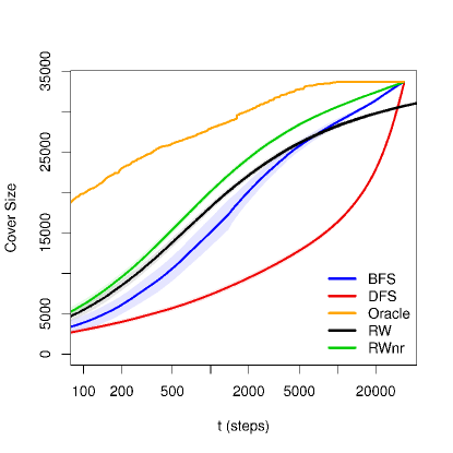
(a)

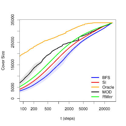
(b)

Figure 2: (Enron Network) Empirical average cover size $\langle\mkern 1.5mu\overline{\mkern-1.5muW\mkern-1.5mu}\mkern 1.5mu(t)\rangle$ as a function of $t\in\{1,N-1\}$. Fig. LABEL:f:BFS_DFS compares Oracle, RW, RWnr, BFS, DFS and Fig. LABEL:f:GSIMOD compares Oracle, RWnr, SI, BFS, MOD. Shadows show double the standard deviation of $1,\!000$ simulations; $x$-axis in log-scale.

Fig. LABEL:f:BFS_DFS shows the average cover size $\langle\mkern 1.5mu\overline{\mkern-1.5muW\mkern-1.5mu}\mkern 1.5mu(t)\rangle$ of BFS and DFS as a function of $t$ on the Enron email network (recall that we average over $1,\!000$ simulation runs). We find similar results on all of our social network datasets, see Figs. LABEL:f:sociala-f. The simulations show while both BFS and DFS achieve the full coverage for $t\approx N$, BFS significantly outperforms DFS for all other values of $t$. To understand this difference, we qualitatively analyze the step in which a given node $v\in V$ with degree $k_{v}$ is recruited.

Because both BFS and DFS follow edges to recruit nodes, the probability that $v$ is first observed in $\mathcal{N}(\mathcal{B}(t))$ at step $t$ is approximately $(\gamma_{v}/N)(1-\gamma_{v}/N)^{t-1}$, where $\gamma_{v}=k_{v}/\langle k\rangle$ (this simple formula should be a good approximation in a configuration model where nodes are recruited independently by both algorithms; it also assumes $t\ll N$). Thus, large degree nodes tend to be observed earlier in the process than small degree nodes. As a FIFO policy recruits the earliest observed nodes from $\mathcal{N}(\mathcal{B}(t))$, BFS tends to recruit large degree nodes first, on the other hand, a LIFO policy recruits the latest observed nodes from $\mathcal{N}(\mathcal{B}(t))$, hence DFS tends to recruit small degree nodes first. This DFS result contradicts previous results in the literature [MaiyaKDD], which we revisit in Sec. LABEL:sec:related.

Note that Fig. LABEL:f:BFS_DFS shows larger standard deviations for BFS than for DFS (although in some social networks the relative difference may be small). This is because the cover size of a non-neglegible fraction of the BFS runs deviates from the average. This instability is due to the strong dependence of the BFS cover size on the initial node $\mathcal{B}(0)=\{i\}$. As BFS explores the network in “waves” (expanding rings from $i$), the initial node selection may significantly impact BFS’s cover size. Moreover, we expect BFS to perform poorly on networks with a large degree of homophily (as seen at the end of Sec. 6 in a simple regular lattice example). Homophily is the tendency of individuals to connect to similar individuals [MSC], thus creating patches of clustered nodes in the network. This means that if $v\in V$ is connected to $u\in V$ and $z\in V$, then $u$ and $z$ are more likely to be connected than random chance would allow. In addition, if $v$ is not connected to $w\in V$ then $u$ and $z$ are more likely than random not to be connected to $w$. In such scenario it pays not to recruit both $u$ and $z$ together, as their neighbors significantly overlap with higher probability than random chance alone would allow.

DFS clearly avoids the above homophily problem by traversing the graph in depth first order. To increase the cover set size we only need to modify the LIFO recruitment policy without resorting to BFS’s FIFO policy. In what follows (Sec. 6) we explore the use of Random Walks (RWs). As we see in the next section, a RW share commonalities with DFS in that it also traverses the graph from the last recruited node (however, a RW may try to recruit a node more than once). But, different from DFS, it allows recruitment of observed nodes in $\mathcal{N}(\mathcal{B}(t))$ irrespective of when the node was observed. One drawback of RWs – that fortunately can be easily mitigated via caching – is the possibility of recruiting already recruited nodes.

6 RW Algorithms

Now let us analyze the cover size of Random Walks (RWs) with one-hop lookahead. Increased attention has been paid to random walks as a tool for network sampling [RT10, Krista, Salganik, Kurant11, KurantJSAC2_11] mostly due to its good statistical properties. In the RW algorithm $\mathcal{N}(\mathcal{B}(t))$ is still the set of all observed unrecruited nodes at time $t$. However, in a RW the node to be recruited at step $t+1$ is a random neighbor of the node recruited at step $t$, regardless of the time that the node was observed or even if it was already recruited. We begin our analysis assuming that a node that is recruited again at step $t$ needs to be paid (that is, time advances even if no new recruitments were performed). We refer to this traditional RW algorithm as RW with replacement (RW), in which nodes already recruited can be recruited again. At the end of this section we extend our analysis to the case of RW without replacement (RWnr) where already recruited nodes are “cached” so that recruiting nodes from $\mathcal{B}(t)$ does not count towards the recruitment budget.

The cover size of RWs with one-hop lookahead has been the subject of previous work [MST06]. However, we feel that one needs to exercise caution when interpreting the results in Mihail et al. [MST06]. Mihail et al. shows that a RW with one-hop lookahead finds the majority of nodes in sublinear time in an infinite configuration model with heavy tailed power law degree distribution. As our approach demonstrates below, covering finite networks is patently different from covering infinite networks. In particular, we show that for any given finite sized network, the discovery rate is never superlinear (this linear growth rate, however, can be large). Our model also allows us to predict with high accuracy the expected number of covered nodes as a function of $0<t\leq n$.

Let us first analyze the performance of RW. In RW, the expected cover size at step $t$ is

$$\langle\mkern 1.5mu\overline{\mkern-1.5muW\mkern-1.5mu}\mkern 1.5mu(t)\rangle =N-\sum_{\forall v\in V}P[\mbox{node $v$ is uncovered}]$$ (1)

$$=N-{\bf q}\sum_{\forall v\in V}\ {}_{\mathcal{N}_{a}(v)}{\bf P}^{t}\underline{1},$$

where ${\bf q}$ is a vector with the initial distribution of the random walk, $\underline{1}$ is a column vector of ones, and ${}_{\mathcal{N}_{a}(v)}{\bf P}$ is a taboo transition probability matrix defined by [_N_a(v)P]_ij= { p_ij,if  i,j ／∈N(v),0,otherwise, with ${\mathcal{N}_{a}}(v)$ denoting the neighborhood set of node $v$, including node $v$.

The above formula (1) requires complete topology knowledge and does not allow simple analytical solution. However, consider the following approximation to a RW. Nodes are recruited with replacement in i.i.d. fashion according to the stationary distribution of the random walk. Then, the expected cover size at step $t$ would be given by

$$\langle\mkern 1.5mu\overline{\mkern-1.5muW\mkern-1.5mu}\mkern 1.5mu(t)\rangle =N-\sum_{\forall v\in V}P[\mbox{node $v$ is uncovered}]$$ (2)

$$=N-\sum_{\forall v\in V}(1-\alpha_{v})^{t},$$

where α_v = 12M (k_v + ∑_j ∈N_a(v) k_j). The above can be interpreted as a particular case of the coupon subset collection problem [AR01, M77]. Each step $t$, $t=1,\ldots,N-1$, we draw a subset of “coupons”, a subset of newly observed nodes in our terminology. We can observe a node either by sampling it directly (this corresponds to the term $k_{v}/(2M)$) or by sampling one of its neighbors (this corresponds to the term $\sum_{j\in\mathcal{N}_{a}(v)}k_{j}/(2M)$). The value of $k_{v}+\sum_{j\in\mathcal{N}_{a}(v)}k_{j}$ is known as the second neighbor degree [Adamic]. In Appendix LABEL:appx:RW we use matrix perturbation theory to show that (2) well approximates (1) for fast mixing RWs (see [ART10, RT10] for fast mixing RW techniques).

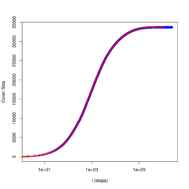
Figure 3: (Enron email) Theoretical RW cover (red line) against simulations (blue circles) on Enron email network. Plots in semi-log scale.

Applying the Taylor series expansion and the fact that $2M=\langle k\rangle N$, we can write – for small $t$ – the following approximation ⟨ ¯W (t) ⟩ ≈t⟨k ⟩N ∑_∀v ∈V