Goldman Algebra, Opers
and the Swapping Algebra

Abstract.

We define a Poisson Algebra called the swapping algebra using the intersection of curves in the disk. We interpret a subalgebra of the fraction algebra of the swapping algebra – called the algebra of multifractions – as an algebra of functions on the space of cross ratios and thus as an algebra of functions on the Hitchin component as well as on the space of $\mathsf{SL}_{n}(\mathbb{R})$-opers with trivial holonomy. We relate this Poisson algebra to the Atiyah–Bott–Goldman symplectic structure and to the Drinfel’d–Sokolov reduction. We also prove an extension of Wolpert formula.

1. Introduction

The purpose of this article is threefold. We first introduce the swapping algebra which is a Poisson algebra generated – as a commutative algebra – by pairs of points on the circle. Then we relate this construction to two well known Poisson structures:

• the Poisson structure of the character variety of representations of a surface group in $\mathsf{PSL}_{n}(\mathbb{R})$ discovered by Atiyah, Bott and Goldman [1, 8, 9]

• the Poisson structure of the space of $\mathsf{PSL}_{n}(\mathbb{R})$-opers introduced by Dickey, Gel’fand and Magri and described in a geometrical way by Drinfel’d and Sokolov [22, 6, 5]

One way to interpret heuristically these relations is to say that the swapping algebra embodies the notion of a “Poisson structure” for the space of all cross ratios, space that contains both the space of opers and the “universal (in genus) Hitchin component”. As a byproduct of the methods of this paper, we also produce a generalisation of the Wolpert formula which computes the brackets of length functions for the Hitchin component.

The results of this article were announced in [19] The relation – at a topological level – between the character variety and opers was already noted by the author in [16], by Fock and Goncharov in [7] and foreseen by Witten in [30] (see also [10, 11]). I thank Martin Bridson, Sergei Fomin, Louis Funar and Bill Goldman for their interest and help.

We now explain more precisely the content of this article.

1.1. The swapping algebra

Our first result is the construction of the swapping algebra. To avoid cumbersome expressions, we shall denote most of the time the ordered pair $(X,x)$ of points of the circle by the concatenated symbol $Xx$. We recall in Paragraph 2.1 the definition and properties of the linking number $[Xx,Yy]$ of the two pairs $(X,x)$ and $(Y,y)$. If $\mathsf{P}$ is a subset of the circle, we denote by $\mathcal{L}(\mathsf{P})$ the commutative associative algebra generated by pairs of points of $\mathsf{P}$ with the relations $XX=0$, for all $X$ in $\mathsf{P}$. Our starting result is the following

Theorem 1.

[Swapping Bracket] For every complex number $\alpha$, there exists a unique Poisson bracket on $\mathcal{L}(\mathsf{P})$ such that the bracket of two generators is

$$\{Xx,Yy\}_{\alpha}{}\mathrel{\mathop{:}}={}[Xx,Yy](Xy.Yx+\alpha.Xx.Yy).$$

The swapping algebra is the algebra $\mathcal{L}_{\alpha}(\mathsf{P})$ endowed with the Poisson bracket $\{\cdotp,\cdotp\}_{\alpha}$. This theorem is proved in Section 2. The goal of this paper is to relate this swapping algebra to other Poisson algebras.

One should note that this bracket can be used to express very simply some results of Wolpert and in particular the variation of the length of curve transverse to a shear [32, 31].

1.2. Cross ratios and the multifraction algebra

We shall concentrate on the interpretation of an offshoot of the swapping algebra. We denote by $\mathcal{Q}_{\alpha}(\mathsf{P})$ the algebra of fractions of $\mathcal{L}_{\alpha}(\mathsf{P})$ equipped with the induced Poisson structure. The multifraction algebra $\mathcal{B}(\mathsf{P})$ is the vector subspace of $\mathcal{Q}_{\alpha}(\mathsf{P})$ generated by the elementary multifractions:

$$[{\rm X},{\rm x};\sigma]{}\mathrel{\mathop{:}}={}\frac{\prod_{i=1}^{i=n}X_{i}x_{\sigma(i)}}{\prod_{i=1}^{i=n}X_{i}x_{i}},$$

where ${\rm X}=(X_{1},\ldots,X_{n})$ and ${\rm x}=(x_{1},\ldots,x_{n})$ are $n$ tuples of points of $\mathsf{P}$ and $\sigma$ is a permutation of $\{1,\ldots,n\}$. Then we have the easy proposition

Proposition 2.

The multifraction algebra is a Poisson subalgebra of $\mathcal{Q}_{\alpha}(\mathsf{P})$. The induced Poisson structure does not depend on $\alpha$. Finally $\mathcal{B}(\mathsf{P})$ is generated as a commutative algebra by the cross fractions:

$$[X,Y,x,y]{}\mathrel{\mathop{:}}={}\frac{Xx.Yy}{Yx.Xy}.$$

In particular, it follows that the multifraction algebra is naturally mapped to the commutative algebra of functions on cross ratios (See Section 3). Thus the existence of a Poisson structure on the multifraction algebra can be interpreted as that of a Poisson structure on the space of cross ratios.

1.3. The multifraction algebra as a “universal” Goldman algebra

We then relate the multifraction algebra to the Goldman algebra. Let $\Gamma$ be the fundamental group of a surface $S$, $\partial_{\infty}\Gamma$ the boundary at infinity of $\Gamma$, and $\mathsf{P}$ be the subset of $\partial_{\infty}\Gamma$ consisting of fixed points of elements of $\Gamma$. The Hitchin component ${\mathsf{H}}(n,S)$ of the character variety of representations of $\Gamma$ in $\mathsf{PSL}_{n}(\mathbb{R})$ was interpreted in [17] as a space of cross ratios. Thus every multifraction in $\mathcal{B}({\mathsf{P}})$ gives a smooth function on the Hitchin component (see Proposition 4.2.4 for details). Thus we have a restriction

$${\mathsf{I}}_{S}:\mathcal{B}(\mathsf{P})\to C^{\infty}({\mathsf{H}}(n,S)).$$

This mapping is not a Poisson morphism, nevertheless it becomes so when we take sequences of well chosen finite index subgroups. More precisely, we define and prove, as an immediate consequence of one of the main result of Niblo in [23], the existence of vanishing sequences of finite index subgroups $\{\Gamma_{n}\}_{n\in\mathbb{N}}$ of $\Gamma$; these sequences are essentially such that every geodesic becomes eventually simple and for which the intersection of two geodesics becomes eventually minimal (See Paragraph 6.2.1 and Appendix 11 for precisions).

Then denoting by $\{\cdotp,\cdotp\}_{W}$ the swapping bracket and $\{\cdotp,\cdotp\}_{S_{n}}$ the Goldman bracket for $S_{n}{}\mathrel{\mathop{:}}={}\tilde{S}/\Gamma_{n}$ coming from the Atiyah–Bott–Goldman symplectic form on the character variety, we prove in Section 9

Theorem 3.

[Goldman bracket for vanishing sequences ]

Let $\{{\Gamma}_{m}\}_{m\in\mathbb{N}}$ be a vanishing sequence of subgroups of $\pi_{1}(S)$. Let $\mathsf{P}\subset\partial_{\infty}\pi_{1}(S)$ be the set of end points of geodesics. Let $b_{0}$ and $b_{1}$ be two multifractions in $\mathcal{B}(\mathsf{P})$. Then we have,

$$\lim_{n\rightarrow\infty}\{b_{0},b_{1}\}_{{S}_{n}}=\{b_{0},b_{1}\}_{W}.$$ (1)

The statement of this theorem actually requires some preliminaries in defining properly the meaning of Assertion (1). In a way, this result tells us that the swapping bracket is the Goldman bracket on the universal solenoid.

The proof relies on the description of special multifractions called elementary functions (see Paragraph 4.2) as limits of the well studied functions on the character variety known as Wilson loops.

Another result is a precise asymptotic formula, on a fixed surface this time, relating the Goldman and the swapping brackets. Let $\Gamma$ be as above. Let $\gamma\in\Gamma$. Let finally $y\in\mathsf{P}$, and $\gamma^{+}$, $\gamma^{-}$ be respectively the attractive and repulsive fixed points of $\gamma$ in $\partial_{\infty}(\Gamma)$. Let us define the following formal series of cross fractions, reverting to the notation $(X,x)$ for pairs,

$$\hat{\ell}_{\gamma}(y)=\frac{1}{2}\log\left(\frac{(\gamma^{+},\gamma(y))\cdot(\gamma^{-},\gamma^{-1}(y))}{(\gamma^{+},\gamma^{-1}(y))\cdot(\gamma^{-},\gamma(y))}\right)$$

In [16] we show that the period function $\ell_{\gamma}{}\mathrel{\mathop{:}}={}{\mathsf{I}}_{S}(\hat{\ell}_{\gamma}(y)))$ – seen as a function on the character variety – is independent on $y$ and is a function of the eigenvalues of the monodromy of $\gamma$. These period functions coincide with the length functions for the classical Teichmüller Theory – that is $n=2$.

We now have

Theorem 4.

[Bracket of length functions] Let $\gamma$ and $\eta$ be homotopy classes of curves which as simple curves have at most one intersection point, then we have

$$\lim_{n\to\infty}{\rm I}_{S}(\{\hat{\ell}_{\gamma^{n}}(y),\hat{\ell}_{\eta^{n}}(y)\}_{W})=\frac{1}{4}\{\ell_{\gamma},\ell_{\eta}\}_{S}$$

As a tool of the proof of this result we prove the following extension of the Wolpert formula [32, 31]

Theorem 5.

[Generalised Wolpert Formula] Let $\gamma$ and $\eta$ be two homotopy classes of curves which as simple curves have exactly one intersection point. Then the Goldman bracket of the two length functions $\ell_{\gamma}$ and $\ell_{\eta}$ is

$$\{\ell_{\gamma},\ell_{\eta}\}_{S}({\bf b})={\iota}(\gamma,\eta)\sum_{\varepsilon,\varepsilon^{\prime}\in\{-1,1\}}\varepsilon\varepsilon^{\prime}.{\bf b}\left(\gamma^{\varepsilon},\eta^{\varepsilon^{\prime}},\gamma^{-\varepsilon},\eta^{-\varepsilon^{\prime}}\right).$$ (2)

This Formula has recently been extended using different methods par Bridgeman in [3].

1.4. The multifraction algebra and $\mathsf{PSL}_{n}(\mathbb{R})$-opers

We finally relate the multifraction algebra to opers. We recall in Section 10 the definition of real opers and their interpretation as maps to the projective space $\mathbb{P}(\mathbb{R}^{n})$ and its dual. In particular, opers with trivial holonomy can be embedded in the space of smooth cross ratios. The Drinfel’d-Sokolov reduction allows us to define the Poisson bracket of pairs of acceptable observables, a subclass of functions on the spaces of opers. We then show that this Poisson bracket coincide with the swapping bracket

Theorem 6.

[Swapping Bracket and opers]

Let $(X_{0},x_{0},Y_{0},y_{0},X_{1},x_{1},Y_{1},y_{1})$ be pairwise distinct points on the circle $\mathbb{T}$. Then the cross fractions $[X_{0},x_{0},Y_{0},y_{0}]$ and $[X_{1},x_{1},Y_{1},y_{1}]$ defines a pair of acceptable observables whose Poisson bracket with respect to the Drinfel’d-Sokolov reduction coincides with their Poisson bracket in the multifraction algebra.

Contents

1. 1 Introduction
   1. 1.1 The swapping algebra
   2. 1.2 Cross ratios and the multifraction algebra
   3. 1.3 The multifraction algebra as a “universal” Goldman algebra
   4. 1.4 The multifraction algebra and $\mathsf{PSL}_{n}(\mathbb{R})$-opers
2. 2 The swapping bracket
   1. 2.1 Linking number for pairs of points
      1. 2.1.1 Properties of the linking number
   2. 2.2 The swapping algebra
   3. 2.3 The multifraction algebra
      1. 2.3.1 Cross fractions and multifractions
      2. 2.3.2 The multifraction algebra
3. 3 Cross ratios and cross fractions
   1. 3.1 Cross ratios
   2. 3.2 Multifractions as functions
   3. 3.3 Multifractions and Hitchin components
      1. 3.3.1 Hitchin component
      2. 3.3.2 Rank $n$ cross ratios
4. 4 Wilson loops, multifractions and length functions
   1. 4.1 Wilson loops
      1. 4.1.1 Asymptotics of Wilson loops
   2. 4.2 Elementary functions
   3. 4.3 The swapping bracket of elementary functions
   4. 4.4 Length functions
      1. 4.4.1 Length functions from the point of view of the multifraction algebra
      2. 4.4.2 Length functions and the character variety
5. 5 The Goldman algebra
   1. 5.1 The Atiyah-Bott-Goldman symplectic form
   2. 5.2 Wilson loops and the Goldman algebra
6. 6 Vanishing sequences and the main results
   1. 6.1 Poisson brackets of length functions
   2. 6.2 Poisson brackets of multifractions
      1. 6.2.1 Vanishing sequences
      2. 6.2.2 Sequences of subgroups and limits
      3. 6.2.3 Poisson brackets of multifractions
7. 7 Product formulas and bouquet in good position
   1. 7.1 An alternative formulation of the Goldman bracket
   2. 7.2 The product formula
      1. 7.2.1 A preliminary case
      2. 7.2.2 Proof of Proposition 7.2.1
   3. 7.3 Bouquets in good position and the product formula
      1. 7.3.1 Bouquets in good position
      2. 7.3.2 Product formula for bouquets
   4. 7.4 Bouquets and covering
   5. 7.5 Finding bouquets in good position
8. 8 Asymptotics
   1. 8.1 Properties of vanishing sequences
      1. 8.1.1 Proof of Proposition 8.1.2
   2. 8.2 Asymptotic product formula for Wilson loops
      1. 8.2.1 Preliminary asymptotics
      2. 8.2.2 Asymptotics and bouquets
      3. 8.2.3 Proof of Proposition 8.2.4
      4. 8.2.4 Proof of Proposition 8.2.1
   3. 8.3 Asymptotics of brackets of multifractions
      1. 8.3.1 Proof of Proposition 8.3.1
9. 9 Goldman and swapping algebras: proofs of the main results
   1. 9.1 Poisson brackets of elementary functions and the proof of Theorem 6.2.4
   2. 9.2 Poisson brackets of length functions
      1. 9.2.1 A generalised Wolpert Formula
      2. 9.2.2 Proof of Theorem 6.1.1
10. 10 Drinfel’d-Sokolov reduction
    1. 10.1 Opers and non-slipping connections
       1. 10.1.1 Opers
       2. 10.1.2 Non-slipping connections
    2. 10.2 The Poisson structure on the space of connections
       1. 10.2.1 Connections and central extensions
       2. 10.2.2 The Poisson structure
    3. 10.3 Drinfel’d-Sokolov reduction
       1. 10.3.1 Dual Lie algebras
       2. 10.3.2 Drinfel’d-Sokolov reduction
    4. 10.4 Opers and Frenet curves
       1. 10.4.1 Curves associated to $\mathsf{PSL}_{n}(\mathbb{R})$-opers
       2. 10.4.2 Hitchin opers
       3. 10.4.3 Frenet curves
    5. 10.5 Cross ratios and opers
       1. 10.5.1 Coordinate functions
       2. 10.5.2 Differential of coordinate functions
    6. 10.6 Poisson brackets on the space of connections
       1. 10.6.1 Regularisation
       2. 10.6.2 Poisson brackets of regularisation
    7. 10.7 Drinfel’d-Sokolov reduction and the multifraction algebra
       1. 10.7.1 Cross ratios
       2. 10.7.2 The main Theorem
11. 11 Appendix: existence of vanishing sequences

2. The swapping bracket

In this section, we first recall the properties and definition of the linking number of two ordered pairs of points. We then construct the swapping algebra and prove Theorem 1 which relies on an identity involving the linking numbers of six points.

2.1. Linking number for pairs of points

We recall that if $(X,x,Y,y)$ is a quadruple of points on the real line the linking number of $(X,x)$ and $(Y,y)$ is

$$[Xx,Yy] {}\mathrel{\mathop{:}}={} \frac{1}{2}\big{(}\operatorname{Sign}(X-x)\operatorname{Sign}(X-y)\operatorname{Sign}(y-x)$$ (4)

$$-\operatorname{Sign}(X-x)\operatorname{Sign}(X-Y)\operatorname{Sign}(Y-x)\big{)},$$

where $\operatorname{Sign}(x)=-1,0,1$ whenever $x<0$, $x=0$ and $x>0$ respectively. By definition, the linking number is invariant by orientation preserving homeomorphisms of the real line.

1. When the four points are pairwise distinct, this linking number is also the total linking number of the curve joining $X$ to $x$ with the curve joining $Y$ to $y$ in the upper half plane.

2. The equality cases are as follows:

   1. For all points $(X,Y,y)$ on the circle

      $$[XX,Yy]=0=[Xy,Xy]\,.$$ (5)

   2. If, up to cyclic permutation, $(X,Y,x)$ are pairwise distinct points and oriented, then

      $$[Xx,Yx]=1/2\,.$$ (6)

The first observation shows that we can define the linking number of a quadruple of points on the oriented circle $S^{1}$ by choosing a point $x_{0}$ disjoint from the quadruple and defining the linking number as the linking number of the quadruple in $S^{1}\setminus\{x_{0}\}\sim\mathbb{R}$. The linking number so defined does not depend on the choice of $x_{0}$ and is invariant under orientation preserving homeomorphisms.

2.1.1. Properties of the linking number

We abstract the useful property (for us) of the linking number of pairs of points in the following definition. Let ${\mathsf{P}}$ be any set.

Definition 2.1.1.

A linking number on pair of points of ${\mathsf{P}}$ is a map from ${\mathsf{P}}^{4}$ to a commutative ring

$$(X,x,Y,y)\to[Xx,Yy],$$

so that for all points $X,x,Y,y,Z,z$

$$[Xx,Yy]+[Yy,Xx] =0\ ,$$ First antisymmetry, (7)

$$[Xx,Yy]+[Xx,yY] =0\ ,$$ Second antisymmetry, (8)

$$[zy,XY]+[zy,YZ]+[zy,ZX] =0\ ,$$ Cocycle identity, (9)

and moreover if $(X,x,Y,y)$ are all pairwise distinct then

$$\ \ \ \ \ \ \ \ \ \ \ \ [Xx,Yy].[Xy,Yx] =0\ ,$$ Linking number alternative. (10)

We illustrate the cocycle identity and the alternative for the standard linking number in Figure (1)

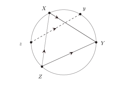
(a) Cocycle identity

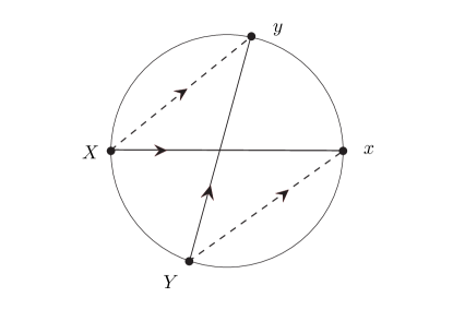
(b) Linking number alternative

Figure 1. linking number for pairs of points on the circle

Then we prove

Proposition 2.1.2.

The canonical linking number for pairs of points of the circle is a linking number in the sense of the previous definition.

Proof.

The first two symmetries are checked from the definition. When $\{x,y\}\cap\{X,Y,Z\}=\emptyset$, then Equation (9) follows from the geometric definition of the linking number. It remains to check different cases of equality. We can assume that $(X,Y,Z)$ are pairwise distinct: otherwise the equality follows from the two previous ones and Assertion (5).

• if $x=y$, the equation is true by Assertion (5).

• Assume that up to cyclic permutations of $(X,Y,Z)$ we have $x=X$ and $y\not\in\{X,Y,Z\}$, then the equality follows from the following remark. Let $z,t$ be points close enough to $x$ so that $(z,x,t)$ is oriented then when $A=Y$ or $A=Z$, we have

  $$[xy,xA]=\frac{1}{2}\left([zy,xA]+[ty,xA]\right).$$

• Assume finally that $(x,y)=(X,Y)$, the the equality reduces to

  $$[XY,ZX]+[XY,YZ]=0,$$

  which is true, by Equation (6) and the fact that $(X,Y,Z)$ has the opposite orientation of $(Y,X,Z)$.

Equation (10) follows from the geometric definition of linking number. ∎

A linking number satisfies more complicated relations. Namely

Proposition 2.1.3.

Let $(X,x,Z,z,Y,y)$ be 6 points on the set ${\mathsf{P}}$ equipped with a linking number $[\cdotp,\cdotp]$, then

$$[Xy,Zz]+[Yx,Zz]=[Xx,Zz]+[Yy,Zz].$$ (11)

Moreover, if

$$\{X,x\}\cap\{Y,y\}\cap\{Z,z\}=\emptyset,$$

then

$$[Xx,Yy][Xy,Zz]+[Zz,Xx][Zx,Yy]+[Yy,Zz][Yz,Xx] =0\ ,$$ (12)

$$[Xx,Yy][Yx,Zz]+[Zz,Xx][Xz,Yy]+[Yy,Zz][Zy,Xx] =0\ .$$ (13)

Remarks:

1. We remark that the hypothesis on the configuration of points is necessary: if $X,x,Y,Z$ are pairwise distinct, then for $(X,x,Y,y,Z,z)=(X,x,Y,x,Z,x)$ the left hand side in Equation (12) is non-zero in the case of the standard linking number of pairs of points on the circle.

2. A simple way to prove this proposition is to use a mathematical computing software, we give below a mathematical proof.

Proof.

Formula (11) follows at once from the Cocycle Identity (9). We now prove Formulas (12) and (13). Let us define

$$F(X,x,Y,y,Z,z) {}\mathrel{\mathop{:}}={}[Xx,Yy][Xy,Zz]+[Zz,Xx][Zx,Yy]+[Yy,Zz][Yz,Xx]\ ,$$

$$G(X,x,Y,y,Z,z) {}\mathrel{\mathop{:}}={}[Xx,Yy][Yx,Zz]+[Zz,Xx][Xz,Yy]+[Yy,Zz][Zy,Xx]\ .$$

We first prove some symmetries of $F$ and $G$.

Our first observation is that, using the Antisymmetry (7), we get that

$$F(X,x,Y,y,Z,z)=-G(Y,y,X,x,Z,z).$$ (14)

Thus we only need to prove that $F=0$. STEP 1: The expression $F$ is invariant under all permutations of the pairs $(X,x)$, $(Y,y)$ and $(Z,z)$

Using Equations (11) and (7), we obtain that

$$F(X,x,Y,y,Z,z)\ + \ G(X,x,Y,y,Z,z)$$

$$= \ [Xx,Yy][Yy,Zz]+[Xx,Yy][Xx,Zz]$$

$$+[Zz,Xx][Zz,Yy]+[Zz,Xx][Xx,Yy]$$

$$+[Yy,Zz][Yy,Xx]+[Yy,Zz][Zz,Xx]$$

$$=0\ .$$

Hence, by Equation (14).

$$F(X,x,Y,y,Z,z)=F(Y,y,X,x,Z,z)$$ (15)

By construction $F$ is invariant by cyclic permutations and thus from the previous equation $F$ is invariant by all permutations of the pairs $(X,x)$,$(Y,y)$ and $(Z,z)$.

STEP 2: The expression $F$ satisfies a cocycle equation

$$F(X,x,Y,y,Z,z)+F(x,t,Y,y,Z,z)=F(X,t,Y,y,Z,z).$$ (16)

We also have the symmetries

$$F(X,x,Y,y,Z,z) =-F(x,X,Y,y,Z,z)$$ (17)

$$=-F(X,x,y,Y,Z,z)$$ (18)

$$=-F(X,x,Y,y,z,Z).$$ (19)

The Symmetries (19) follow at once from the Cocycle (16) and the fact that $F(X,X,Y,y,Z,z)=0$.

Let us prove a cocycle equation for $F$. We shall only use the cocycle Equation (9) and the previous symmetries for the linking number. By definition,

$$F(X,x,Y,y,Z,z)\ + \ F(x,t,Y,y,Z,z)$$

$$= \ \ [Xx,Yy][Xy,Zz]+[xt,Yy][xy,Zz]$$

$$+[Zz,Xx][Zx,Yy]+[Zz,xt][Zt,Yy]$$

$$+[Yy,Zz][Yz,Xx]+[Yy,Zz][Yz,xt].$$

Using the cocycle Equation (9) to expand the first and regrouping the fifth and sixth terms of the right hand side, we get

$$F(X,x,Y,y,Z,z)\ + \ F(x,t,Y,y,Z,z)$$

$$= \ \ [Xt,Yy][Xy,Zz]+[tx,Yy][Xy,Zz]+[xt,Yy][xy,Zz]$$

$$+[Zz,Xx][Zx,Yy]+[Zz,xt][Zt,Yy]$$

$$+[Yy,Zz][Yz,Xt].$$

Using the cocycle Equation (9) for regrouping the second and third term of the right hand side and rearranging, we get

$$F(X,x,Y,y,Z,z)\ + \ F(x,t,Y,y,Z,z)$$

$$= \ \ [Xt,Yy][Xy,Zz]$$

$$+[Zz,Xx][Zx,Yy]+[Zz,Xx][xt,Yy]+[Zz,xt][Zt,Yy]$$

$$+[Yy,Zz][Yz,Xt]$$

$$= \ F(X,t,Y,y,Z,z).$$

Using the cocycle Equation (9) to regroup the second and third term, then the fourth, of the right hand side, we finally get

$$F(X,x,Y,y,Z,z)\ + \ F(x,t,Y,y,Z,z)$$

$$= \ \ [Xt,Yy][Xy,Zz]$$

$$+[Zz,Xt][Zt,Yy]$$

$$+[Yy,Zz][Yz,Xt]$$

$$= \ F(X,t,Y,y,Z,z).$$

STEP 3: If $(X,x,Y,y)$ are pairwise distinct, then

$$F(X,x,Y,y,Y,x) =0\,,$$ (20)

$$F(X,x,X,x,Y,y) =0\,.$$ (21)

Let us prove first Equation (20). It follows from the Alternative (10) and the cocycle Equation (9) that

$$F(X,x,Y, y,Y,x)$$

$$=[Xx,Yy][Xy,Yx]+([Yx,Xx][Yx,Yy]+[Yy,Yx][Yx,Xx])$$

$$=0\ .$$

This proves Formula (20). Similarly, using the cocycle Formula (16) for $F$ for the first equality, symmetries for the second and our previous Formula (20) (for $(X,x,y,Y)$ ) for the last, we get

$$F(X,x,X, x,Y,y)$$

$$=F(X,x,X,y,Y,y)+F(X,x,y,x,Y,y)$$

$$=F(X,x,y,x,y,Y)=F(X,x,y,Y,y,x)$$

$$=0.$$

STEP 4: If $(X,x,Y,y,Z)$ are pairwise distinct, then

$$F(X,x,Y, y,Z,x)=0\,.$$ (22)

Using the cocycle Formula (16) for $F$ and the previous step, we get

$$F(X,x,Y, y,Z,x)$$

$$=F(X,x,Y,Z,Z,x)+F(X,x,Z,y,Z,x)$$

$$=-F(X,x,Z,Y,Z,x)=0\ .$$

FINAL STEP: If $(X,x,Y,y,Z,z)$ are pairwise distinct, then

$$F(X,x,Y, y,Z,z)=0\,.$$ (23)

Indeed, using the cocycle Formula (16) for $F$ for the first equality, symmetries for the second, and the previous step for the last equality, we get

$$F(X,x,Y, y,Z,z)$$

$$=F(X,x,Y,y,Z,Y)+F(X,x,Y,y,Y,z)$$

$$=F(y,Y,x,X,Z,Y)-F(y,Y,x,X,y,z,Y)$$

$$=0\ .$$

This concludes the proof. ∎

2.2. The swapping algebra

Let ${\mathsf{P}}$ be a set and $[\cdotp,\cdotp]$ be a linking number with values in an integral domain $A$. We represent a pair $(X,x)$ of points of ${\mathsf{P}}$ by the expression $Xx$. We consider the free associative commutative algebra $\mathcal{L}({\mathsf{P}})$ generated over $A$ by pair of points on ${\mathsf{P}}$, together with the relation $XX=0$ for all $X\in\mathsf{P}$.

Let $\alpha$ be any element in $A$. We define the swapping bracket of two pairs of points as the following element of $\mathcal{L}({\mathsf{P}})$

$$\{Xx,Yy\}_{\alpha}{}\mathrel{\mathop{:}}={}[Xx,Yy](\alpha.Xx.Yy+Xy.Yx).$$ (24)

We extend the swapping bracket to the whole algebra $\mathcal{L}({\mathsf{P}})$ using the Leibniz Rule and call the resulting algebra $\mathcal{L}_{\alpha}({\mathsf{P}})$ the swapping algebra.

Theorem 2.2.1.

The swapping bracket satisfies the Jacobi identity. Hence, the swapping algebra $\mathcal{L}_{\alpha}({\mathsf{P}})$ is a Poisson algebra.

Proof.

All we need to check is the Jacobi identity

$$\{\{Xx,Yy\}_{\alpha},Zz\}_{\alpha}+\{\{Yy,Zz\}_{\alpha},Xx\}_{\alpha}+\{\{Zz,Xx\}_{\alpha},Yy\}_{\alpha}=0,$$

for the generators of the algebra.

We make preliminary computations, omitting the subscript $\alpha$ in the bracket. The triple bracket $\{\{A,B\},C\}$ is a polynomial of degree 2 in $\alpha$ and we wish to compute its coefficients. By definition, using the Leibniz rule for the second equality, we have

$$\{\{Xx,Yy\},Zz\}= [Xx,Yy]\left(\alpha\{Xx.Yy,Zz\}+\{Xy.Yx,Zz\}\right)$$ (25)

$$= \ \alpha[Xx,Yy]\left(\{Xx,Zz\}.Yy+\{Yy,Zz\}.Xx\right)$$ (26)

$$+[Xx,Yy]\left(\{Xy,Zz\}.Yx+\{Yx,Zz\}.Xy\right).$$ (27)

Now we compute two expressions appearing in the right hand side of the previous equation. We have

$$\{Xx,Zz\}.Yy\ +\ \{Yy,Zz\}.Xx$$ (28)

$$=\ \alpha\left([Xx,Zz]+[Yy,Zz]\right)Xx.Yy.Zz$$ (29)

$$+\left([Xx,Zz]Xz.Yy.Zx+[Yy,Zz]Xx.Yz.Zy\right).$$ (30)

Similarly

$$\{Xy,Zz\}.Yx+\ \{Yx,Zz\}.Xy$$ (31)

$$= \alpha\left([Xy,Zz]+[Yx,Zz]\right)Xy.Yx.Zz$$ (32)

$$+[Xy,Zz]Xz.Yx.Zy+[Yx,Zz]Xy.Yz.Zx\,.$$ (33)

It follows from Equations (30) and (33) that the coefficient of $\alpha^{2}$ in the triple bracket (27) is

$$P_{2}{}\mathrel{\mathop{:}}={}\left([Xx,Yy][Xx,Zz]+[Xx,Yy][Yy,Zz]\right)Xx.Yy.Zz.$$ (34)

The coefficient of $\alpha$ in the triple bracket (27) is

$$P_{1}{}\mathrel{\mathop{:}}={}\ \ =\ \ [Xx,Yy][Xx,Zz]Xz.Yy.Zx+[Xx,Yy][Yy,Zz]Xx.Yz.Zy$$ (35)

$$+([Xx,Yy][Xy,Zz]+[Xx,Yy][Yx,Zz])Xy.Yx.Zz.$$ (36)

Finally the constant coefficient is

$$P_{0} {}\mathrel{\mathop{:}}={}[Xx,Yy][Xy,Zz]Xz.Yx.Zy+[Xx,Yy][Yx,Zz]Xy.Yz.Zx,$$ (37)

so that

$$\{\{Xx,Yy\},Zz\}= \alpha^{2}P_{2}+\alpha.P_{1}+P_{0}.$$ (38)

In order to check the Jacobi identity, we have to consider the sum $S_{2}$, $S_{1}$ and $S_{0}$ over cyclic permutations of $(Xx,Yy,Zz)$ of the three terms $P_{2}$, $P_{1}$ and $P_{0}$. We consider successively these three coefficients.

Term of degree 0: We first have

$$S_{0} =F(X,x,Y,y,Z,z)(Xz.Yx.Zy-Xy.Yz.Zx)\ ,$$ (39)

Indeed, we have

$$S_{0} =A.Xz.Yx.Zy+B.Xy.Yz.Zx\ ,$$

where

$$A =[Xx,Yy][Xy,Zz]+[Zz,Xx][Zx,Yy]+[Yy,Zz][Yz,Xx]=F(X,x,Y,y,Z,z)\ ,$$

$$B =[Xx,Yy][Yx,Zz]+[Zz,Xx][Xz,Yy]+[Yy,Zz][Zy,Xx]=G(X,x,Y,y,Z,z)\ .$$

Now Equation (39) follows from Equation (14). We now prove that $S_{0}=0$. It follows from Proposition 2.1.3 that if

$$\{X,x\}\cap\{Y,y\}\cap\{Z,z\}=\emptyset,$$

then $F=0$, hence $S_{0}=0$.

Up to cyclic permutations, we just have to consider two cases

1. If $x=y=z$ or $X=Y=Z$ then

   $$Xz.Yx.Zy-Xy.Yz.Zx=0,$$

   hence $S_{0}=0$.

2. If $x=y=Z$ or $X=Y=z$ or the other cases obtained by cyclic permutations, since $aa=0$, we have

   $$Xz.Yx.Zy=Xy.Yz.Zx=0$$

   Thus $S_{0}=0$.

We have completed the proof that $S_{0}=0$. Term of degree 1. Next, we write

$$P_{1}= \ A_{1}(X,x,Y,y,Z,z)Xx.Yz.Zy$$

$$+A_{2}(X,x,Y,y,Z,z)Xz.Yy.Zx$$

$$+A_{3}(X,x,Y,y,Z,z)Xy.Yx.Zz\ .$$

Thus

$$S_{1} =A_{x}.Xx.Yz.Zx+A_{y}.Xz.Yy.Zx.+A_{z}.Xy.Yx.Zz\ ,$$

where

$$A_{z}= A_{3}(X,x,Y,y,Z,z)+A_{2}(Y,y,Z,z,X,x)+A_{1}(Z,z,X,x,Y,y)$$

$$= \ [Xx,Yy][Xy,Zz]+[Xx,Yy][Yx,Zz]$$

$$+[Yy,Zz][Yy,Xx]+[Zz,Xx][Xx,Yy]$$

$$= \ [Xx,Yy]\left([Xy,Zz]+[Yx,Zz]-[Yy,Zz]-[Xx,Zz]\right)\ .$$

By Equation (11), $A_{z}=0$. Therefore, $A_{y}=A_{z}=A_{x}=0$ by cyclic permutations. We have completed the proof that $S_{1}=0$. Term of degree 2. Finally, $S_{2}=C.Xx.Yy.Zz$, where

$$C= \ [Xx,Yy][Xx,Zz]+[Xx,Yy][Yy,Zz]$$

$$+[Yy,Zz][Yy,Xx]+[Yy,Zz][Zz,Xx]$$

$$+[Zz,Xx][Zz,Yy]+[Zz,Xx][Xx,Yy]\ .$$

Then $C=0$ by the antisymmetry of the linking number. Thus $S_{2}=0$.

This concludes the proof of the Jacobi identity. Indeed

$$\{\{Xx,Yy\}_{\alpha},Zz\}_{\alpha}+\{\{Yy,Zz\}_{\alpha},Xx\}_{\alpha}+ \{\{Zz,Xx\}_{\alpha},Yy\}_{\alpha}$$

$$=\alpha^{2}S_{2}+\alpha S_{1}+S_{0}$$

$$=0.$$

∎

2.3. The multifraction algebra

The swapping algebra is very easy to define. However, in the sequel we shall need to consider other Poisson algebras built out of the swapping algebra: these algebras will be more precisely subalgebras of the fraction algebra of $\mathcal{L}(\mathsf{P})$. We introduce in this paragraph cross fractions, multifractions and the multifraction algebra.

2.3.1. Cross fractions and multifractions

Since $\mathcal{L}_{\alpha}(\mathsf{P})$ is an integral domain (with respect to the commutative product) we can consider its algebra of fractions $\mathcal{Q}_{\alpha}(\mathsf{P})$.

Let $(X,Y,x,y)=:Q$ be a quadruple of points of $\mathsf{P}$ so that $x\not=Y$ and $y\not=X$. The cross fraction determined by $Q$ is the element of $\mathcal{Q}_{\alpha}(\mathsf{P})$ defined by

$$[X;Y;x;y]{}\mathrel{\mathop{:}}={}\frac{Xx.Yy}{Xy.Yx}.$$

More generally, let ${\rm X}{}\mathrel{\mathop{:}}={}(X_{1},\ldots,X_{n})$ and ${\rm x}{}\mathrel{\mathop{:}}={}(x_{1},\ldots x_{n})$ are two tuples of elements of $\mathsf{P}$ so that $x_{i}\not=X_{i}$ for all $i$, let $\sigma$ be a permutation of $\{1,\ldots,n\}$ then the elementary multifraction – defined over $\mathsf{P}$ – defined by this data is

$$[{\rm X},{\rm x};\sigma]{}\mathrel{\mathop{:}}={}\frac{\prod_{i=1}^{i=n}X_{i}x_{\sigma(i)}}{\prod_{i=1}^{i=n}X_{i}x_{i}}.$$

2.3.2. The multifraction algebra

Let now $\mathcal{B}(\mathsf{P})$ be the vector space generated by elementary multifractions and let us call any element of $\mathcal{B}(\mathsf{P})$ a multifraction. We have the following proposition

Proposition 2.3.1.

The vector space $\mathcal{B}(\mathsf{P})$ is a Poisson subalgebra of $\mathcal{Q}_{\alpha}(\mathsf{P})$. Moreover it is generated as a Poisson algebra by cross fractions. Finally the swapping bracket $\{\cdotp,\cdotp\}_{\alpha}$ when restricted to $\mathcal{B}(\mathsf{P})$ does not depend on $\alpha$.

From now on, we call the Poisson algebra $\mathcal{B}(\mathsf{P})$ the algebra of multifractions.

Proof.

The proposition follows from the following immediate observations:

• every elementary multifraction is a product of cross fractions,

• if $A$ and $B$ are two cross fractions then $\{A,B\}_{\alpha}$ is a multifraction and does not depend on $\alpha$.

∎

3. Cross ratios and cross fractions

In this section, we interpret cross fractions, and in general multifractions, as functions on the space of cross ratios.

3.1. Cross ratios

Recall that a cross ratio on a set ${\mathsf{P}}$ is a map $\mathbf{b}$ from

$${\mathsf{P}}^{4*}{}\mathrel{\mathop{:}}={}\{(X,Y,x,y)\in{\mathsf{P}}\mid y\not=X,x\not=Y\}$$

to a field $\mathbb{K}$ which satisfies some algebraic rules. These rules encode two conditions which constitute a normalisation, and two multiplicative cocycle identities which hold for different sets of variables:

$${\hbox{\sc Normalisation:}}\ \ \mathbf{b}(X,Y,x,y) = 0\ \ \Leftrightarrow x=X\,,\hbox{ or }Y=y,$$

$${\hbox{\sc Normalisation:}}\ \ \mathbf{b}(X,Y,x,y) = 1\ \ \Leftrightarrow x=y\,,\hbox{ or }X=Y,$$

$${\hbox{\sc Cocycle identity:}}\ \ \mathbf{b}(X,Y,x,y) = {\mathbf{b}(X,Y,x,z)}{\mathbf{b}(X,Y,z,y)},$$

$${\hbox{\sc Cocycle identity:}}\ \ \mathbf{b}(X,Y,x,y) = \mathbf{b}(X,Z,x,y)\mathbf{b}(Z,Y,x,y).$$

Assume $\Gamma$ acts on ${\mathsf{P}}$, way say the cross ratio $\mathbf{b}$ is $\Gamma$-invariant, if it is invariant under the diagonal action.

Remarks:

• We change our convention from our previous articles [16, 17] in order to be coherent with the formula for the classical projective cross ratio: let $\mathbf{b}$ be a cross ratio with respect to the definition above, let $b(X,x,Y,y){}\mathrel{\mathop{:}}={}\mathbf{b}(X,Y,x,y)$, then $b$ is a cross ratio using our older convention. Observe that the second normalisation together with the cocycle identities imply the following symmetries:

  $$\mathbf{b}(X,Y,x,y)=\mathbf{b}(Y,X,x,y)^{-1}=\mathbf{b}(Y,X,y,x)=\mathbf{b}(X,Y,y,x)^{-1}.$$

• Assume $\Gamma$ acts on ${\mathsf{P}}$. Let $\mathbf{b}$ be a $\Gamma$-invariant cross ratio. Let $\gamma\in\Gamma$ and $\gamma^{+}$ and $\gamma^{-}$ be two $\gamma$-fixed points in ${\mathsf{P}}$, then the following quantity

  $$\mathbf{b}(\gamma^{+},\gamma^{-},\gamma y,y)$$

  does not depends on the choice of $y$. In particular, let $S$ be a closed connected oriented surface of genus greater than 2, let ${\mathsf{P}}$ be $\partial_{\infty}\pi_{1}(S)$ equipped with the action of $\pi_{1}(S)$. Let $\gamma^{+}$ and $\gamma^{-}$ be respectively the attractive and repulsive fixed point of a non-trivial element $\gamma$ of $\pi_{1}(S)$ and $\mathbf{b}$ a $\pi_{1}(S)$-invariant cross ratio, then

  $$\ell_{\mathbf{b}}(\gamma){}\mathrel{\mathop{:}}={}\left|\log\left|\mathbf{b}(\gamma^{+},\gamma^{-},\gamma(y),y)\right|\right|,$$

  is called the period of $\gamma$.

We finally denote by $\mathds{B}(\mathsf{P})$ the set of cross ratios on $\mathsf{P}$.

These definitions are closely related to those given by Otal in [24, 25], discussions from various perspectives by Ledrappier in [21] and work of Bourdon in [2] in the context of ${\rm CAT}(-1)$-spaces.

3.2. Multifractions as functions

To every cross fraction $[X;Y;x;y]$, we associate a function, denoted by $\overline{[X;Y;x;y]}$, on $\mathds{B}(\mathsf{P})$ by the following formula

$$\overline{[X;Y;x;y]}(\mathbf{b}){}\mathrel{\mathop{:}}={}\mathbf{b}(X,Y,x,y).$$

The following proposition follows at once from the definition of cross ratio

Proposition 3.2.1.

The map ${[X;Y;x;y]}\to\overline{[X;Y;x;y]}$ extends uniquely to a morphism of commutative associative algebras from $\mathcal{B}(\mathsf{P})$ to the algebra of functions on $\mathds{B}(\mathsf{P})$.

In the sequel, we shall use an identical notation for a multifraction and its image in the space of functions on $\mathds{B}(\mathsf{P})$. So far also, we did not (and will not) consider any topological structure on $\mathds{B}(\mathsf{P})$ nor on $\mathsf{P}$.

3.3. Multifractions and Hitchin components

In [16], we identified the Hitchin component with a space of cross ratios satisfying certain identities. Let us recall notation and definitions

3.3.1. Hitchin component

Let $S$ be a closed oriented connected surface with genus at least two.

Definition 3.3.1.

[Fuchsian and Hitchin homomorphisms] An $n$-Fuchsian homomorphism from $\pi_{1}(S)$ to $\mathsf{PSL}_{n}(\mathbb{R})$ is a homomorphism $\rho$ which factorises as $\rho={{\iota}}\circ\rho_{0}$, where $\rho_{0}$ is a discrete faithful homomorphism with values in $\mathsf{PSL}_{2}(\mathbb{R})$ and ${{\iota}}$ is an irreducible homomorphism from $\mathsf{PSL}_{2}(\mathbb{R})$ to $\mathsf{PSL}_{n}(\mathbb{R})$.

An $n$-Hitchin homomorphism from $\pi_{1}(S)$ to $\mathsf{PSL}_{n}(\mathbb{R})$ is a homomorphism which may be deformed into an $n$-Fuchsian homomorphism

The Hitchin component ${{\mathsf{H}}(n,S)}$ is the space of Hitchin homomorphisms up to conjugacy by an exterior automorphism of $\mathsf{PSL}_{n}(\mathbb{R})$. All these representations lift to $\mathsf{SL}(n,\mathbb{R})$. By construction ${{\mathsf{H}}(n,S)}$ is identified with a connected component of the character variety. It is a result by Hitchin [15] that ${{\mathsf{H}}(n,S)}$ is homeomorphic to the interior of a ball of dimension $(2g-2)(n^{2}-1)$.

As a corollary of the main result of [16], we have

Theorem 3.3.2.

If $\rho$ is Hitchin, if $\gamma$ is a non-trivial element of $\pi_{1}(S)$ then $\rho(\gamma)$ has $n$ distinct positive real eigenvalues.

By convention, we write these eigenvalues as $\lambda_{1}(\rho(\gamma)),\ldots,\lambda_{n}(\rho(\gamma))$ where

$$\lambda_{1}(\rho(\gamma))>\ldots>\lambda_{n}(\rho(\gamma))>0.$$

This allows us to introduce the following

Definition 3.3.3.

[Girth and width] The width of a non-trivial element $\gamma$ of $\pi_{1}(S)$ with respect to a Hitchin representation $\rho$ is

$$\operatorname{width}_{\rho}(\gamma){}\mathrel{\mathop{:}}={}\log\left(\left|\frac{\lambda_{1}(\rho(\gamma))}{\lambda_{n}(\rho(\gamma))}\right|\right).$$

The girth of $\rho$ is

$$\operatorname{gh}(\rho){}\mathrel{\mathop{:}}={}\sup\left\{\left|\frac{\lambda_{2}(\rho(\gamma))}{\lambda_{1}(\rho(\gamma))}\right|\mid\gamma\in\pi_{1}(S)\setminus\{{\rm Id}\}\right\}.$$ (40)

The following proposition will be used several times

Proposition 3.3.4.

Let $C$ be a compact subset of ${\mathsf{H}}(n,S)$ then

1. For any positive $A$, the following subset of $\pi_{1}(S)$ defined by

   $$S_{A}=\left\{\gamma\in\pi_{1}(S)\mid\exists\rho\in C,\,\,\left|\frac{\lambda_{2}(\rho(\gamma))}{\lambda_{1}(\rho(\gamma))}\right|>A\right\}$$

   contains only finitely many conjugacy classes.

2. Moreover

   $$\sup\{\operatorname{gh}(\rho)\mid\rho\in C\}<1.$$

For the proof of this proposition, we first need

Lemma 3.3.5.

Let $S$ be a hyperbolic surface with unit tangent bundle $\mathsf{U}S$ equipped with the geodesic flow $\{\phi_{t}\}_{t\in\mathbb{R}}$. Let $\rho_{0}$ be a Hitchin representation in ${\mathsf{H}}(n,S)$. Then there exists a neighbourhood $W$ of $\rho_{0}$ in ${\mathsf{H}}(n,S)$, such that for every $\rho$ in $W$, there exists a function $f_{\rho}:\mathsf{U}S\to\mathbb{R}$ verifying

• for every closed orbit $\gamma$ and $x\in\gamma$,

  $$\int_{0}^{\ell(\gamma)}f_{\rho}\circ\phi_{s}(x)\,{\rm d}s\,=\log\left|\frac{\lambda_{1}(\rho(\gamma))}{\lambda_{2}(\rho(\gamma))}\right|,$$

  where $\ell(\gamma)$ is the hyperbolic length of $\gamma$;

• the function $\rho\mapsto f_{\rho}$ is continuous from $W$ to $C^{0}(\mathsf{U}S,\mathbb{R})$ and moreover there exists a positive constant $\varepsilon_{0}$ so that for all $\rho$, $f_{\rho}>\varepsilon_{0}$ .

.

Proof of Lemma 3.3.5: This follows from the Anosov property of Hitchin representations and results in [4]. One could also use results by Guichard–Wienhard [14] or combine results of Sambarino [27, 26]. Since by Theorem 6.1 of [4], the limit maps of a Hitchin representation depend in an analytic way of the representation, we can find

• a neighbourhood $D$ of $\rho_{0}$ in ${\mathsf{H}}(n,S)$,

• a vector bundle $E$ over $M{}\mathrel{\mathop{:}}={}D\times\mathsf{U}S$ smooth along $\mathsf{U}S$,

• a splitting of $E=L_{1}\oplus\ldots L_{n}$ into line bundles smooth along the geodesic flow,

• a continuous lift $\{\Phi_{t}\}_{t\in\mathbb{R}}$ on $E$ of the geodesic flow $\{\phi_{t}\}_{t\in\mathbb{R}}$ on $M$ preserving this decomposition and smooth along $\mathsf{U}S$,

so that if $\gamma$ is a closed geodesic of hyperbolic length $\ell(\gamma)$ and $u\in L_{i}|_{\{\rho\}\times\gamma}$, then

$$\Phi_{\ell(\gamma)}(u)=\lambda_{i}(\rho(\gamma))\cdotp u.$$

In this last equation, we identify the closed geodesic with the corresponding conjugacy class in $\pi_{1}(S)$. We now construct metrics $\omega_{i}$ on $L_{i}$ smooth along the geodesic flow. Let us consider the functions $g_{i}$ on $M$ so that $g_{i}\cdotp\omega_{i}=\left.\frac{\rm d}{{\rm d}t}\right|_{t=0}\Phi_{t}^{*}\omega_{i}$. In particular, we have

$$\Phi_{t}^{*}\omega_{i}(x)=\exp\left(\int_{0}^{t}g_{i}\circ\phi_{s}(x)\,{\rm d}s\right)\omega_{i}(x).$$ (41)

Then by construction for $x\in\{\rho\}\times\gamma$, we have

$$-\log\left(\lambda_{i}(\rho(\gamma)\right)=\int_{0}^{\ell(\gamma)}g_{i}\circ\phi_{s}(x)\,{\rm d}s.$$

Let now $g=g_{2}-g_{1}$, then

$$\log\left(\frac{\lambda_{1}(\rho(\gamma))}{\lambda_{2}(\rho(\gamma))}\right)=\int_{0}^{\ell(\gamma)}g\circ\phi_{s}(x)\,{\rm d}s.$$

By the Anosov property, there exists some $T>0$, so that the flow $\Phi_{T}$ contracts uniformly on $\operatorname{Hom}(L_{1},L_{2})$ along $\{\rho_{0}\}\times\mathsf{U}S$. In a more precise way, if we denote by $\omega_{1}^{*}$ the dual metric on $L_{1}^{*}$ to $\omega_{1}$, then there exists some $T$ so that along $\{\rho_{0}\}\times\mathsf{U}S$, we have

$$\Phi_{T}^{*}(\omega_{1}^{*}\otimes\omega_{2})=H\cdotp\omega_{1}^{*}\otimes\omega_{2},$$

where $H$ is a continuous function on $M$ so that along $\{\rho_{0}\}\times\mathsf{U}S$,

$$H<\frac{1}{2}.$$

By the continuity of $H$, the previous inequality extends to $M$ after possibly restricting $D$. As a consequence, we have for $x\in M$,

$$\int_{0}^{T}g\circ\phi_{s}(x)\,{\rm d}s=-\log(H(x))>\log(2).$$

Let now

$$f(x){}\mathrel{\mathop{:}}={}\frac{1}{T}\int_{0}^{T}g\circ\phi_{s}(x)\,{\rm d}s.$$

Then by construction

$$f(x)>\frac{1}{T}\log(2){}=\mathrel{\mathop{:}}{}\varepsilon_{0},$$

and, moreover, for $x\in\{\rho\}\times\mathsf{U}S$,

$$\int_{0}^{\ell(\gamma)}f\circ\phi_{s}(x)\,{\rm d}s=\int_{0}^{\ell(\gamma)}g\circ\phi_{s}(x)\,{\rm d}s=\log\left(\frac{\lambda_{1}(\rho(\gamma))}{\lambda_{2}(\rho(\gamma))}\right).$$

∎

Proof of Proposition 3.3.4: By compactness, it is enough to prove that every $\rho$ in ${\mathsf{H}}(n,S)$ possesses a neighbourhood $W$ so that the properties of the proposition hold when $C$ is replaced by $W$. We choose the neighbourhood $W$ obtained in the previous lemma. Let then $f_{\rho}$ be as in the conclusion of this lemma. Since $f_{\rho}$ is bounded away from zero by a positive constant $\varepsilon_{0}$, it follows that

$$\log\left(\frac{\lambda_{1}(\rho(\gamma))}{\lambda_{2}(\rho(\gamma))}\right)>\varepsilon_{0}\cdot\,\ell(\gamma).$$

The first result immediately follows. Then for the second result we use the fact that $S_{\frac{1}{2}}$ contains only finitely many conjugacy classes and that given $\gamma$ the function

$$\rho\mapsto\frac{\lambda_{2}(\rho(\gamma))}{\lambda_{1}(\rho(\gamma))},$$

is continuous and with values less than 1. ∎

3.3.2. Rank $n$ cross ratios

For every integer $p$, let $\partial_{\infty}\pi_{1}(S)^{p}_{*}$ be the set of pairs

$$({\rm X},{\rm x})=\left((X_{0},X_{1},\ldots,X_{p}),(x_{0},x_{1},\ldots,x_{p})\right),$$

of $(p+1)$-tuples of points in $\partial_{\infty}\pi_{1}(S)$ such that $X_{j}\not=X_{i}\not=x_{0}$ and $x_{j}\not=x_{i}\not=X_{0}$, whenever $j>i>0$. Let $\chi^{p}({\rm X},{\rm x})$ be the multifraction defined by

$$\chi^{p}({\rm X},{\rm x}){}\mathrel{\mathop{:}}={}\det_{i,j>0}\left([X_{i};X_{0};x_{j};x_{0}]\right).$$

A cross ratio $\mathbf{b}$ has rank $n$ if

• $\chi^{n}({\rm X},{\rm x})(\mathbf{b})\not=0$, for all $({\rm X},{\rm x})$ in $\partial_{\infty}\pi_{1}(S)^{n}_{*}$,

• $\chi^{n+1}({\rm X},{\rm x})(\mathbf{b})=0$, for all $({\rm X},{\rm x})$ in $\partial_{\infty}\pi_{1}(S)^{n+1}_{*}$.

The main result of [18] – which used a result by Guichard [13] – is the following.

Theorem 3.3.6.

There exists a bijection $\phi$ from the set of $n$-Hitchin representations to the set of $\pi_{1}(S)$-invariant rank $n$ cross ratios, such that if $\mathbf{b}=\phi(\rho)$ then

1. for any non-trivial element $\gamma$ of $\pi_{1}(S)$

   $$\ell_{\mathbf{b}}(\gamma)=\operatorname{width}_{\rho}(\gamma),$$

   where $\ell_{\mathbf{b}}(\gamma)$ is the period of $\gamma$ given with respect to $\mathbf{b}=\phi(\rho)$, and $\operatorname{width}_{\rho}(\gamma)$ is the width of $\gamma$ with respect to $\rho$.

2. Moreover, if $\gamma_{1}$ and $\gamma_{2}$ are two non-trivial elements of $\pi_{1}(S)$, if $e_{i}$, (respectively $E_{i}$) is an eigenvector of $\rho(\gamma_{i})$ of maximal eigenvalue (respectively eigenvector of $\rho^{*}(\gamma_{i})$ of minimum eigenvalue) then

   $$\mathbf{b}(\gamma_{1}^{+},\gamma_{2}^{+},\gamma_{2}^{-},\gamma_{1}^{-}) = \frac{\langle E_{2},e_{1}\rangle\langle E_{1},e_{2}\rangle}{\langle E_{1},e_{1}\rangle\langle E_{2},e_{2}\rangle}.$$ (42)

In particular, every multifraction defines a function on the Hitchin component.

4. Wilson loops, multifractions and length functions

In this section, we shall relate Wilson loops – which are regular functions on the character variety – to multifractions. We will also introduce elementary functions which are limits of Wilson loops, prove that they generate the multifraction algebra and that they are smooth functions on the Hitchin component. We finally introduce length functions in Paragraph 4.4.

4.1. Wilson loops

Let $\gamma$ be an element of $\pi_{1}(S)$ and $\rho$ be an element of ${\mathsf{H}}(n,S)$. The Wilson loop associated to $\gamma$ is the function ${\mathsf{W}}(\gamma)$ on ${\mathsf{H}}(n,S)$ defined by

$${\mathsf{W}}(\gamma)(\rho){}\mathrel{\mathop{:}}={}\operatorname{tr}(\rho(\gamma)).$$

Wilson loops only depends on conjugacy classes. Let us introduce the following definition.

Definition 4.1.1.

[Class of an element] Let $\gamma$ be a non-trivial element of $\pi_{1}(S)$, the class $[\gamma]$ of $\gamma$ is the oriented pair $(\gamma^{+},\gamma^{-})$ of points of $\partial_{\infty}\pi_{1}(S)$ where $\gamma^{+}$ and $\gamma^{-}$ are respectively the attractive and repulsive fixed points of $\gamma$.

Recall that $[\gamma]=[\eta]$ if and only if there exist positive integers $m$ and $n$ so that $\gamma^{m}=\eta^{n}$.

4.1.1. Asymptotics of Wilson loops

Let $\rho$ be a Hitchin representation. Recall that for any $\gamma$ in $\pi_{1}(S)$ we can write

$$\rho(\gamma)=\sum_{1\leqslant i\leqslant n}\lambda_{i}(\rho(\gamma))p_{i}(\gamma),$$

where $p_{i}(\gamma)$ is a projector of trace 1, and $\lambda_{i}(\rho(\gamma))$ are real numbers so that

$$0<|\lambda_{n}(\rho(\gamma))|<\ldots<|\lambda_{1}(\rho(\gamma))|.$$

Let us denote $\accentset{\bullet}{\rho}(\gamma)=p_{1}(\gamma)$. We denote by $[\mathsf{A}]$ the set of eigenvectors of a purely loxodromic matrix $\mathsf{A}$, and observe that $[\mathsf{A}^{n}]=[\mathsf{A}]$. We choose an auxiliary norm, denoted $\|\cdotp\|$ on $\mathbb{R}^{n}$. Then we have

Proposition 4.1.2.

For any $\gamma$ in $\pi_{1}(S)$, and $p\in\mathbb{N}$ we have

$$\left\|\frac{\rho(\gamma^{p})}{{\mathsf{W}}(\gamma^{p})(\rho)}-\accentset{\bullet}{\rho}(\gamma)\right\| \leqslant \operatorname{gh}(\rho)^{p}K\left([\rho(\gamma)]\right),$$ (43)

where $K$ is a continuous function on the set of $n$ lines in general position.

Proof.

Let $\mathsf{A}=\rho(\gamma)$. Since ${\mathsf{A}}$ is a real diagonalisable matrix then

$${\mathsf{A}}=\sum_{i=1}^{i=n}\lambda_{i}{\mathsf{p}}_{i},$$

where ${\mathsf{p}}_{i}$ are projectors and the eigenvalues $\lambda_{i}$ satisfy $\lambda_{1}>\cdots>\lambda_{n}>0$. Thus

$$\left\|\frac{{\mathsf{A}}^{p}}{\operatorname{tr}({\mathsf{A}}^{p})}-{\mathsf{p}}_{1}\right\| \leqslant \frac{1}{\sum_{i=1}^{i=n}\lambda_{i}^{p}}\left\|\sum_{i=2}^{i=n}\lambda_{i}^{p}{\mathsf{p}}_{i}-\left(\sum_{i=2}^{i=n}\lambda_{i}^{p}\right){\mathsf{p}}_{1}\right\|$$ (44)

$$\leqslant \left(\frac{\lambda_{2}}{\lambda_{1}}\right)^{p}\left(n\|{\mathsf{p}}_{1}\|+\sum_{i=2}^{i=n}\|{\mathsf{p}}_{2}\|\right).$$ (45)

Thus the inequality follows by taking

$$K([{\mathsf{A}}])=n\|{\mathsf{p}}_{1}\|+\sum_{i=2}^{i=n}\|{\mathsf{p}}_{2}\|.$$

∎

As a corollary, we get

Corollary 4.1.3.

Let $\gamma_{1}$, $\gamma_{2}$,$\ldots$, $\gamma_{q}$ be $p$ coprime elements of $\Gamma$, let $m_{1}$, $m_{2}$,$\ldots$, $m_{q}$ be positive numbers then

$$\left\|\frac{\prod_{i=1}^{q}\rho(\gamma_{i}^{m_{i}})}{{\mathsf{W}}\left(\prod_{i=1}^{q}\gamma_{i}^{m_{i}}\right)(\rho)}-\frac{\accentset{\bullet}{\rho}(\gamma_{1})\accentset{\bullet}{\rho}(\gamma_{q})}{\operatorname{tr}\left(\accentset{\bullet}{\rho}(\gamma_{1})\accentset{\bullet}{\rho}(\gamma_{q})\right)}\right\| \leqslant \operatorname{gh}(\rho)^{m}K,$$ (46)

where $m=\inf(m_{i})$ and $K$ depends continuously on the eigenvectors of $\rho(\gamma_{i})$ and their relative configurations.

Proof.

We restate the previous Proposition by saying that

$$\rho(\gamma^{p}) = {\mathsf{W}}(\gamma^{p})(\rho)\cdotp\left(\accentset{\bullet}{\rho}(\gamma)+\operatorname{gh}(\rho)^{p}\cdotp K(\gamma,\rho)\right),$$ (47)

where $K(\gamma,\rho)$ is continuous in $\rho$ and only depends on the eigenvectors of $\rho(\gamma)$. Thus

$$\prod_{i=1}^{q}\rho(\gamma_{i}^{m_{i}}) = \prod_{i=1}^{q}{\mathsf{W}}(\gamma_{i}^{m_{i}})(\rho)\cdotp\prod_{i=1}^{q}\left(\accentset{\bullet}{\rho}(\gamma_{i})+\operatorname{gh}(\rho)^{m_{i}}\cdotp K(\gamma_{i},\rho)\right)$$ (48)

$$= \prod_{i=1}^{q}{\mathsf{W}}(\gamma_{i}^{m_{i}})(\rho)\cdotp\left(\prod_{i=1}^{q}\accentset{\bullet}{\rho}(\gamma_{i})+\operatorname{gh}(\rho)^{m}\cdotp K_{0}(\gamma_{1},\ldots,\gamma_{p};\rho)\right),$$ (49)

where $K_{0}(\gamma_{1},\ldots,\gamma_{p};\rho)$ is continuous in $\rho$ and only depends on the eigenvectors of $\rho(\gamma_{i})$. Thus

$$\frac{{\mathsf{W}}\left(\prod_{i=1}^{q}\gamma_{i}^{m_{i}}\right)(\rho)}{\prod_{i=1}^{q}{\mathsf{W}}(\gamma_{i}^{m_{i}})(\rho)} = \operatorname{tr}\left(\prod_{i=1}^{q}\accentset{\bullet}{\rho}(\gamma_{i})\right)+\operatorname{gh}(\rho)^{m}\cdotp K_{1}(\gamma_{1},\ldots,\gamma_{p};\rho),$$ (50)

where $K_{1}(\gamma_{1},\ldots,\gamma_{p};\rho)$ is continuous in $\rho$ and only depends on the eigenvectors of $\rho(\gamma_{i})$. Combining equations (49) and (50), we obtain that

$$\frac{\prod_{i=1}^{q}\rho(\gamma_{i}^{m_{i}})}{{\mathsf{W}}\left(\prod_{i=1}^{q}\gamma_{i}^{m_{i}}\right)(\rho)} = \frac{\prod_{i=1}^{q}\accentset{\bullet}{\rho}(\gamma_{i})}{\operatorname{tr}\left(\prod_{i=1}^{q}\accentset{\bullet}{\rho}(\gamma_{i})\right)}+\operatorname{gh}(\rho)^{m}\cdotp K_{2}(\gamma_{1},\ldots,\gamma_{p};\rho),$$ (51)

where $K_{1}(\gamma_{1},\ldots,\gamma_{p};\rho)$ is continuous in $\rho$ and only depends on the eigenvectors of $\rho(\gamma_{i})$ and their relative positions. To conclude the proof of the corollary, we remark that is $A$ is an endormorphism $\rm p$ and $\rm q$ are projectors so that $\operatorname{tr}({\rm p}A{\rm q})\not=0\not=\operatorname{tr}({\rm p}A{\rm q})$, then

$$\frac{{\rm p}A{\rm q}}{\operatorname{tr}({\rm p}A{\rm q})}=\frac{{\rm p}{\rm q}}{\operatorname{tr}({\rm p}{\rm q})}\ .$$

Using this remark, we get that

$$\frac{\prod_{i=1}^{q}\accentset{\bullet}{\rho}(\gamma_{i})}{\operatorname{tr}\left(\prod_{i=1}^{q}\accentset{\bullet}{\rho}(\gamma_{i})\right)} = \frac{\accentset{\bullet}{\rho}(\gamma_{1})\accentset{\bullet}{\rho}(\gamma_{q})}{\operatorname{tr}\left(\accentset{\bullet}{\rho}(\gamma_{1})\accentset{\bullet}{\rho}(\gamma_{q})\right)}\,.$$

Combining this last equality with Equality (51) yields the statement of the corollary. ∎

We begin with the following proposition where we consider multifractions as functions on ${\mathsf{H}}(n,S)$.

Proposition 4.1.4.

Let $\gamma_{1},\ldots,\gamma_{k}$ be non-trivial elements of $\pi_{1}(S)$. Then the sequence

$$\left\{\frac{{\mathsf{W}}(\gamma_{1}^{p}\ldots\gamma_{k}^{p})}{{\mathsf{W}}(\gamma_{1}^{p})\ldots{\mathsf{W}}(\gamma_{k}^{p})}\right\}_{p\in\mathbb{N}}$$

converges uniformly on every compact of ${\mathsf{H}}(n,S)$ to a multifraction when $p$ goes to infinity. More precisely,

$$\lim_{p\rightarrow\infty}\left(\frac{{\mathsf{W}}(\gamma_{1}^{p}\ldots\gamma_{k}^{p})}{{\mathsf{W}}(\gamma_{1}^{p})\ldots{\mathsf{W}}(\gamma_{k}^{p})}\right)=\frac{\prod_{i=1}^{i=k}\gamma_{i+1}^{+}\gamma_{i}^{-}}{\prod_{i=1}^{i=k}\gamma_{i}^{+}\gamma_{i}^{-}}=[{\rm G}^{+},{\rm G}^{-};\tau],$$

where ${\rm G}^{\pm}=(\gamma_{1}^{\pm},\ldots,\gamma_{k}^{\pm})$ and $\tau(i)=i-1$, using the convention that $k+1=1$.

Proof.

We first observe that if $e_{i}$, (respectively $E_{i}$) is an eigenvector of $\rho(\gamma_{i})$ of maximal eigenvalue (respectively eigenvector of $\rho^{*}(\gamma_{i})$ of minimum eigenvalue) so that $\langle E_{i},e_{i}\rangle=1$ then

$$\operatorname{tr}(\accentset{\bullet}{\rho}(\gamma_{1})\ldots\accentset{\bullet}{\rho}(\gamma_{k}))=\prod_{i}\langle E_{i},e_{i+1}\rangle.$$

By Equation (42),

$$\prod_{i}\langle E_{i},e_{i+1}\rangle=\left(\frac{\prod_{i=1}^{i=p}\gamma_{i+1}^{+}\gamma_{i}^{-}}{\prod_{i=1}^{i=k}\gamma_{i}^{+}\gamma_{i}^{-}}\right)(\rho).$$

It thus follows that

$$\operatorname{tr}(\accentset{\bullet}{\rho}(\gamma_{1})\ldots\accentset{\bullet}{\rho}(\gamma_{k}))=[{\rm G}^{+},{\rm G}^{-};\tau].$$

Then the result follows at once from Propositions 4.1.2 and 3.3.4.∎

4.2. Elementary functions

Proposition 4.1.4 leads us to the following definition.

Definition 4.2.1.

The multifraction

$${\mathsf{T}}(\gamma_{1},\ldots,\gamma_{p}){}\mathrel{\mathop{:}}={}\frac{\prod_{i=1}^{i=p}\gamma_{i+1}^{+}\gamma_{i}^{-}}{\prod_{i=1}^{i=p}\gamma_{i}^{+}\gamma_{i}^{-}}$$ (52)

is an elementary function of order $p$

By the previous proposition and its proof, we have the following equalities

$${\mathsf{T}}(\gamma_{1},\ldots,\gamma_{p}) = \lim_{n\rightarrow\infty}\frac{{\mathsf{W}}(\gamma_{1}^{n}\ldots\gamma_{p}^{n})}{{\mathsf{W}}(\gamma_{1}^{n})\ldots{\mathsf{W}}(\gamma_{p}^{n})}$$ (53)

$${\mathsf{T}}(\gamma_{1},\ldots,\gamma_{p}) = \operatorname{tr}(\accentset{\bullet}{\rho}(\gamma_{1})\ldots\accentset{\bullet}{\rho}(\gamma_{p})).$$ (54)

The following formal properties of elementary functions are then easily checked.

Proposition 4.2.2.

The following properties of elementary functions hold

1. Cyclic invariance: for every cyclic permutation $\sigma$ of $\{1,\ldots,p\}$ we have

   $${\mathsf{T}}(\gamma_{1},\ldots,\gamma_{p})={\mathsf{T}}(\gamma_{\sigma(1)},\ldots,\gamma_{\sigma(p)})$$

2. Class invariance: if $[\eta_{i}]=[\gamma_{i}]$ then

   $${\mathsf{T}}(\gamma_{1},\ldots\gamma_{p})={\mathsf{T}}(\eta_{1},\ldots,\eta_{p}).$$

3. if $[\gamma_{p}]=[\gamma_{p-1}]$ then

   $${\mathsf{T}}(\gamma_{1},\ldots\gamma_{p})={\mathsf{T}}(\gamma_{1},\ldots\gamma_{p-1})$$

4. if $[\gamma_{p}]=[\gamma_{p-1}^{-1}]$ then

   $${\mathsf{T}}(\gamma_{1},\ldots\gamma_{p})=0$$

5. Relations Assume that $[\gamma_{i}]\not=[\gamma_{i+1}]$ then

   $${\mathsf{T}}(\gamma_{1},\ldots,\gamma_{p})=\frac{{\mathsf{T}}(\gamma_{1},\gamma_{2}){\mathsf{T}}(\gamma_{1},\gamma_{p}){\mathsf{T}}(\gamma_{2},\gamma_{3},\ldots,\gamma_{p})}{{\mathsf{T}}(\gamma_{p},\gamma_{2},\gamma_{1})}$$

We deduce from the last statement the following corollary

Corollary 4.2.3.

Let $\mathsf{P}$ be the set of fixed points in $\partial_{\infty}\pi_{1}(S)$ of non-trivial elements of $\pi_{1}(S)$. Then every restriction of an elementary multifraction over $\mathsf{P}$ is a quotient of product of elementary functions of order 2 and 3.

Proof.

Let us consider $a,b,c,d$ be four non-trivial elements of $\pi_{1}(S)$, then we have

$$\frac{{\mathsf{T}}(a,b,c).{\mathsf{T}}(c,d)}{{\mathsf{T}}(a,d,c){\mathsf{T}}(c,b)}=[b^{+};d^{+};a^{-};c^{-}].$$ (55)

The result follows. ∎

Recall that in this section we choose $\mathsf{P}$ to be the set of fixed points of non-trivial elements of $\pi_{1}(S)$. We now prove,

Proposition 4.2.4.

Every multifraction – defined over $\mathsf{P}$ – is a smooth function on ${\mathsf{H}}(n,S)$.

Proof.

Let $\operatorname{Hom}(n,S)$ be the space of Hitchin homomorphisms. Let $\pi$ be the submersion

$$\pi:\operatorname{Hom}(n,S)\to{\mathsf{H}}(n,S)=\operatorname{Hom}(n,S)/\operatorname{Aut}(\mathsf{PSL}_{n}(\mathbb{R})).$$

For every loxodromic element $A$ in $\mathsf{PSL}_{n}(\mathbb{R})$, let $p_{A}$ be the projection on the eigenspace of maximal eigenvalue with respect to the other eigenspaces. The map $A\to p_{A}$ (from the space of loxodromic elements) is smooth. It follows that for any elements $\gamma_{1},\ldots,\gamma_{k}$ in $\pi_{1}(S)$ the map from $\operatorname{Hom}(n,S)$ to $\mathbb{R}$ defined by

$$\Psi:\rho\to\operatorname{tr}(p_{\rho(\gamma_{1})}.\ldots.p_{\rho(\gamma_{k})})$$

is smooth. We conclude by observing that $\Psi$ is $\operatorname{Aut}(\mathsf{PSL}_{n}(\mathbb{R}))$-invariant and that by Equation (54)

$$\Psi={\mathsf{T}}(\gamma_{1},\ldots,\gamma_{k})\circ\pi.$$

Thus every elementary function is smooth and by the previous result every multifraction is smooth. ∎

4.3. The swapping bracket of elementary functions

For the sequel, we shall need to compute the swapping brackets of elementary functions. This is given by the following proposition whose proof follows by an immediate application of the definition. We first say that two non-trivial elements $\gamma$ and $\eta$ in $\pi_{1}(S)$ are coprime if for all non-zero integers $m$ and $n$, $\gamma^{n}\not=\eta^{m}$.

Proposition 4.3.1.

Let $\gamma_{0},\ldots,\gamma_{p}$, respectively $\eta_{0},\ldots,\eta_{q}$ be elements of $\pi_{1}(S)\setminus\{1\}$ such that $(\gamma_{i},\gamma_{i+1})$ as well as $(\eta_{j},\eta_{j+1})$ are pairwise coprime. Let

$${\rm a}_{i,j} {}\mathrel{\mathop{:}}={} [\gamma_{i}^{+}\gamma_{i}^{-},\eta_{j}^{+}\eta_{j}^{-}]\,,$$ (56)

$${\rm b}_{i,j} {}\mathrel{\mathop{:}}={} [\gamma_{i+1}^{+}\gamma_{i}^{-},\eta_{j+1}^{+}\eta_{j}^{-}]\,,$$ (57)

$${\rm c}_{i,j} {}\mathrel{\mathop{:}}={} [\gamma_{i}^{+}\gamma_{i}^{-},\eta_{j+1}^{+}\eta_{j}^{-}]\,,$$ (58)

$${\rm d}_{i,j} {}\mathrel{\mathop{:}}={} [\gamma_{i+1}^{+}\gamma_{i}^{-},\eta_{j}^{+}\eta_{j}^{-}]\,,$$ (59)

$${\mathsf{T}}_{\gamma} {}\mathrel{\mathop{:}}={} {\mathsf{T}}(\gamma_{0},\ldots,\gamma_{p})$$ (60)

$${\mathsf{T}}_{\eta} {}\mathrel{\mathop{:}}={} {\mathsf{T}}(\eta_{0},\ldots,\eta_{q})\,.$$ (61)

Then

$$\frac{\{{\mathsf{T}}_{\gamma},{\mathsf{T}}_{\eta}\}}{{\mathsf{T}}_{\gamma}.{\mathsf{T}}_{\eta}} = \mathop{\sum_{0\leqslant i\leqslant q,}}_{0\leqslant j\leqslant p}\left({\rm a}_{i,j}{\mathsf{T}}(\gamma_{i},\eta_{j})+{\rm b}_{i,j}\frac{{\mathsf{T}}(\eta_{j+1},\eta_{j},\gamma_{i+1},\gamma_{i})}{{\mathsf{T}}(\eta_{j},\eta_{j+1}){\mathsf{T}}(\gamma_{i},\gamma_{i+1})}\right)$$ (62)

$$- \mathop{\sum_{0\leqslant i\leqslant q}}_{0\leqslant j\leqslant p}\left({\rm c}_{i,j}\frac{{\mathsf{T}}(\gamma_{i},\eta_{j+1},\eta_{j})}{{\mathsf{T}}(\eta_{j},\eta_{j+1})}+{\rm d}_{i,j}\frac{{\mathsf{T}}(\eta_{j},\gamma_{i+1},\gamma_{i})}{{\mathsf{T}}(\gamma_{i},\gamma_{i+1})}\right).$$ (63)

Proof.

Using “logarithmic derivatives”, we have

$$\frac{\{{\mathsf{T}}_{\gamma},{\mathsf{T}}_{\eta}\}}{{\mathsf{T}}_{\gamma}.{\mathsf{T}}_{\eta}} =\mathop{\sum_{0\leqslant i\leqslant p,}}_{0\leqslant j\leqslant q}\Bigg{(}\left(\frac{\{\gamma_{i+1}^{+}\gamma_{i}^{-},\eta_{j+1}^{+}\eta_{j}^{-}\}}{\gamma_{i+1}^{+}\gamma_{i}^{-}.\eta_{j+1}^{+}\eta_{j}^{-}}+\frac{\{\gamma_{i}^{+}\gamma_{i}^{-},\eta_{j}^{+}\eta_{j}^{-}\}}{\gamma_{i}^{+}\gamma_{i}^{-}.\eta_{j}^{+}\eta_{j}^{-}}\right)$$

$$-\left(\frac{\{\gamma_{i}^{+}\gamma_{i}^{-},\eta_{j+1}^{+}\eta_{j}^{-}\}}{\gamma_{i}^{+}\gamma_{i}^{-}.\eta_{j+1}^{+}\eta_{j}^{-}}+\frac{\{\gamma_{i+1}^{+}\gamma_{i}^{-},\eta_{j}^{+}\eta_{j}^{-}\}}{\gamma_{i+1}^{+}\gamma_{i}^{-}.\eta_{j}^{+}\eta_{j}^{-}}\right)\Bigg{)}$$

$$=\sum_{\begin{subarray}{c}0\leqslant i\leqslant q\\ 0\leqslant j\leqslant p\end{subarray}}\Bigg{(}{\rm b}_{i,j}\frac{\gamma_{i+1}^{+}\eta_{j}^{-}.\eta_{j+1}^{+}\gamma_{i}^{-}}{\gamma_{i+1}^{+}\gamma_{i}^{-}.\eta_{j+1}^{+}\eta_{j}^{-}}+{\rm a}_{i,j}\frac{\gamma_{i}^{+}\eta_{j}^{-}.\eta_{j}^{+}\gamma_{i}^{-}}{\gamma_{i}^{+}\gamma_{i}^{-}.\eta_{j}^{+}\eta_{j}^{-}}$$

$$-{\rm d}_{i,j}\frac{\gamma_{i+1}^{+}\eta_{j}^{-}.\eta_{j}^{+}\gamma_{i}^{-}}{\gamma_{i+1}^{+}\gamma_{i}^{-}.\eta_{j}^{+}\eta_{j}^{-}}-{\rm c}_{i,j}\frac{\gamma_{i}^{+}\eta_{j}^{-}.\eta_{j+1}^{+}\gamma_{i}^{-}}{\gamma_{i}^{+}\gamma_{i}^{-}.\eta_{j+1}^{+}\eta_{j}^{-}}\Bigg{)}.$$

From the definition of elementary functions (52), we get that

$$\frac{{\mathsf{T}}(\eta_{j+1},\eta_{j},\gamma_{i+1},\gamma_{i})}{{\mathsf{T}}(\eta_{j},\eta_{j+1}){\mathsf{T}}(\gamma_{i},\gamma_{i+1})} = \frac{\gamma_{i+1}^{+}\eta_{j}^{-}.\eta_{j+1}^{+}\gamma_{i}^{-}}{\gamma_{i+1}^{+}\gamma_{i}^{-}.\eta_{j+1}^{+}\eta_{j}^{-}}\,,$$

$${\mathsf{T}}(\gamma_{i},\eta_{j}) = \frac{\gamma_{i}^{+}\eta_{j}^{-}.\eta_{j}^{+}\gamma_{i}^{-}}{\gamma_{i}^{+}\gamma_{i}^{-}.\eta_{j}^{+}\eta_{j}^{-}}\,,$$

$$\frac{{\mathsf{T}}(\eta_{j},\gamma_{i+1},\gamma_{i})}{{\mathsf{T}}(\gamma_{i},\gamma_{i+1})} = \frac{\gamma_{i+1}^{+}\eta_{j}^{-}.\eta_{j}^{+}\gamma_{i}^{-}}{\gamma_{i+1}^{+}\gamma_{i}^{-}.\eta_{j}^{+}\eta_{j}^{-}}\,,$$

$$\frac{{\mathsf{T}}(\gamma_{i},\eta_{j+1},\eta_{j})}{{\mathsf{T}}(\eta_{j},\eta_{j+1})} = \frac{\gamma_{i}^{+}\eta_{j}^{-}.\eta_{j+1}^{+}\gamma_{i}^{-}}{\gamma_{i}^{+}\gamma_{i}^{-}.\eta_{j+1}^{+}\eta_{j}^{-}}.$$

This concludes the proof of the proposition ∎

4.4. Length functions

We introduce in this paragraph length functions.

4.4.1. Length functions from the point of view of the multifraction algebra

Recall first that $\pi_{1}(S)$ acts on $\partial_{\infty}\pi_{1}(S)$ and thus on $\mathcal{B}(\partial_{\infty}\pi_{1}(S))$. For any $y\in\partial_{\infty}\pi_{1}(S)$ and $\beta$ a non-trivial element in $\pi_{1}(S)$, let us introduce the following cross fraction,

$$p_{\beta}(y)=\frac{(\beta^{+},\beta(y))\cdotp(\beta^{-},\beta^{-1}(y))}{(\beta^{+},\beta^{-1}(y))\cdotp(\beta^{-},\beta(y))},$$

where for readibility we revert to the classical notation $(X,x)$ for pair of points rather than the concatenated notation $Xx$. We have, for any $\beta$ in $\pi_{1}(S)$

$$\frac{p_{\beta}(y)}{p_{\beta}(z)}=\frac{(\beta^{2})*F_{y,z}}{F_{y,z}},$$

where

$$F_{y,z}=\frac{(\beta^{+},\beta^{-1}(y))\cdotp(\beta^{-},\beta^{-1}(z))}{(\beta^{+},\beta^{-1}(z))\cdotp(\beta^{-},\beta^{-1}(y))}$$

In particular, the restriction of $p_{\beta}(y)$ to the space of $\pi_{1}(S)$-invariant cross ratios is independent on the choice of $y$.

For the sake of simplicity, we introduce the following formal series of multifractions and call it a length function.

$$\hat{\ell}_{\beta}(y){}\mathrel{\mathop{:}}={}\frac{1}{2}\log(p_{\beta}(y)),$$

extending the bracket by the “log derivative” formulas

$$\{\hat{\ell}_{\beta}(y),q\}{}\mathrel{\mathop{:}}={}\frac{\{p_{\beta}(y),q\}}{2\,p_{\beta}(y)},\ \ \{\hat{\ell}_{\beta}(y),\hat{\ell}_{\gamma}(z)\}{}\mathrel{\mathop{:}}={}\frac{\{p_{\beta}(y),p_{\gamma}(z)\}}{4\,p_{\beta}(y).p_{\gamma}(z)}.$$ (64)

Observe that ${\rm I}_{S}(\hat{\ell}_{\beta^{n}}(y))=n.{\rm I}_{S}(\hat{\ell}_{\beta}(y))$.

4.4.2. Length functions and the character variety

We can further relate these objects with the period and length defined in Paragraph 3.1. Let

$${\rm I}_{S}:\mathcal{B}(\partial_{\infty}\pi_{1}(S))\to C^{\infty}({\mathsf{H}}(n,S)),$$

denote the restriction of functions from $\mathbb{B}(\partial_{\infty}\pi_{1}(S))$ to ${\mathsf{H}}(n,S)$.

We have for $\beta\in\pi_{1}(S)$ that

$${\rm I}_{S}(\hat{\ell}_{\beta}(y))=\ell_{\beta},$$

where

$$\ell_{\beta}(\rho){}\mathrel{\mathop{:}}={}\ell_{b}(\beta),$$

and $\ell_{b}$ is the period of $\beta$ which respect to the cross ratio associated to $\rho$ (see Section 3.1).

5. The Goldman algebra

In this section, we first recall the construction of the Atiyah–Bott–Goldman symplectic form on the character variety. We then explain the construction of the Goldman algebra which allows to compute the bracket of Wilson loops in terms of a Lie bracket on the vector space generated by free homotopy classes of loops.

5.1. The Atiyah-Bott-Goldman symplectic form

In [1], Atiyah and Bott introduced a symplectic structure on the character variety of representations of closed surface groups in compact Lie group, generalising Poincaré duality. This was later generalised by Goldman for non-compact groups in [9, 8] and connected to the Weil–Petersson Kähler form. If we identify the tangent space of ${\mathsf{H}}(n,S)$ at $\rho$ with $H^{1}_{\rho}(\mathfrak{g})$, where $\mathfrak{g}$ is the Lie algebra of $\mathsf{PSL}_{n}(\mathbb{R})$ then the symplectic form is given

$$\omega_{S}\left([A],[B]\right)=\int_{S}\operatorname{tr}(A\wedge B),$$ (65)

where $A$ and $B$ are de Rham representatives of the cohomology classes $[A]$ and $[B]$. We denote by $\{\cdotp,\cdotp\}_{S}$ the associated Poisson bracket, called the Atiyah–Bott–Goldman (ABG) Poisson bracket in the sequel, and $\mathcal{A}(S)$ the Poisson algebra of smooth functions on ${\mathsf{H}}(n,S)$. In the next paragraph, we show how to compute the Atiyah–Bott–Goldman bracket, in the case of $\mathsf{PSL}_{n}(\mathbb{R})$, for the Wilson loops that we introduced in the previous section.

5.2. Wilson loops and the Goldman algebra

We describe in this paragraph the Goldman algebra and how it helps computing the ABG-Poisson bracket. Let $\rm C$ be the set of free homotopy class of closed curves on an oriented surface ${S}$. Let ${\mathbb{Q}}[\rm C]$ be the vector space generated by $\rm C$ over $\mathbb{Q}$. We extend linearly Wilson loops so that the map $\gamma\mapsto{\mathsf{W}}(\gamma)$ is now a linear map from ${\mathbb{Q}}[\rm C]$ to $C^{\infty}({\mathsf{H}}(n,S))$.

Goldman introduced in [9] a Lie bracket on ${\mathbb{Q}}[\rm C]$. We define it for two elements $\gamma_{1}$ and $\gamma_{2}$ of $\rm C\subset\mathbb{Q}[\rm C]$ and then extend it to $\mathbb{Q}[\rm C]$ linearly. We choose two curves representing $\gamma_{1}$ and $\gamma_{2}$, which we denote the same way.

If $\gamma_{1}$ and $\gamma_{2}$ are two curves from $S^{1}$ to $S$, an intersection point is a pair $(a,b)$ in $S^{1}\times S^{1}$ so that $\gamma_{1}(a)=\gamma_{2}(b)$. By a slight abuse of language, we usually identify an intersection point $(a,b)$ with its image $x=\gamma_{1}(a)=\gamma_{2}(b)$. We further assume that $\gamma_{1}$ and $\gamma_{2}$ have transverse intersection points.

For every intersection point $x$, let ${\iota}_{x}$ be the local intersection number at $x$, let $\gamma_{1}\divideontimes_{x}\gamma_{2}$ be the free homotopy class of the curve obtained by composing $\gamma_{1}$ and $\gamma_{2}$ in $\pi_{1}({S},x)$ and finally let

$${\iota}(\gamma_{1},\gamma_{2}){}\mathrel{\mathop{:}}={}\sum_{x\in\gamma_{1}\cap\gamma_{2}}{\iota}_{x},$$

be the global intersection number.

Definition 5.2.1.

The Goldman bracket of $\gamma_{1}$ and $\gamma_{2}$ is the element of $\mathbb{Q}[\rm C]$ defined by

$$\{\gamma_{1},\gamma_{2}\} {}\mathrel{\mathop{:}}={} \sum_{x\in\gamma_{1}\cap\gamma_{2}}{\iota}_{x}\cdotp\gamma_{1}\divideontimes_{x}\gamma_{2}.$$ (66)

We illustrate in Picture 2, the Goldman bracket of two curves.

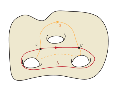
(a) Two curves

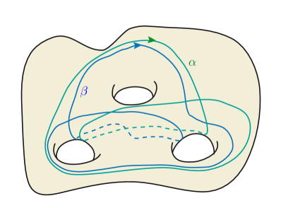
(b) Their Goldman bracket

Figure 2. $\{b,a\}=\alpha-\beta$

Goldman proved in [9] that this bracket does not depend on the choice of representatives and is a Lie bracket. Moreover this bracket is related to the ABG-Poisson bracket as follows.

Theorem 5.2.2.

[Goldman] Let $\gamma_{1}$ and $\gamma_{2}$ be two loops on $S$. Then the ABG-Poisson bracket of the two corresponding Wilson loops in ${\mathsf{H}}(n,S)$ is

$$\{{\mathsf{W}}({\gamma_{1}}),{\mathsf{W}}({\gamma_{2}})\}_{S}={\mathsf{W}}({\{\gamma_{1},\gamma_{2}\}})-\frac{{\iota}(\gamma_{1},\gamma_{2})}{n}{\mathsf{W}}({\gamma_{1}})\cdotp{\mathsf{W}}({\gamma_{2}})\,.$$ (67)

We just stated Goldman theorem for the case of ${\mathsf{H}}(n,S)$, but the theorem has a formulation in the general case of character varieties for semi-simple groups. A different proof can also be found in [20].

6. Vanishing sequences and the main results

In this section, we first recall the definition of the length functions on the character varieties, introduce the notion of a vanishing sequence of finite index subgroups of a surface group and state our main results relating the swapping algebra to the Goldman algebra. All these results will be proved in Section 9. Let as usual

$${\rm I}_{S}:\mathcal{B}(\partial_{\infty}\pi_{1}(S))\to C^{\infty}({\mathsf{H}}(n,S)),$$

denote the restriction of functions from $\mathbb{B}(\partial_{\infty}\pi_{1}(S))$ to ${\mathsf{H}}(n,S)$.

6.1. Poisson brackets of length functions

We explain in this section our results concerning length functions (See Paragraph 4.4 for notations and definitions). Our first result relates the Goldman and the swapping Poisson bracket.

Theorem 6.1.1.

Let $\gamma$ and $\eta$ be two geodesics with at most one intersection point, then we have

$$\lim_{n\to\infty}{\rm I}_{S}(\{\hat{\ell}_{\gamma^{n}}(y),\hat{\ell}_{\eta^{n}}(y)\})=\frac{1}{4}\{\ell_{\gamma},\ell_{\eta}\}_{S}\,.$$

In the course of the proof of this result, we prove the following result of independent interest which is an extension of Wolpert Formula [32, 31]

Theorem 6.1.2.

[Generalised Wolpert Formula].

Let $\gamma$ and $\eta$ two closed geodesics with a unique intersection point then the Goldman bracket of the two length functions $\ell_{\gamma}$ and $\ell_{\eta}$ seen as functions on the Hitchin component is

$$\{\ell_{\gamma},\ell_{\eta}\}_{S}={\iota}(\gamma,\eta)\sum_{\varepsilon,\varepsilon^{\prime}\in\{-1,1\}}\varepsilon\varepsilon^{\prime}.{\mathsf{T}}(\gamma^{\varepsilon}.\eta^{\varepsilon^{\prime}}),$$ (68)

where we recall that

$${\mathsf{T}}(\xi,\zeta)(\rho)=\mathbf{b}_{\rho}(\xi^{+},\zeta^{+},\zeta^{-},\xi^{-}).$$

We prove these two results in Paragraph 9.2

6.2. Poisson brackets of multifractions

We now relate in general the swapping bracket and the Goldman bracket. Our result can be described by saying that the swapping bracket is an inverse limit (with respect to sequences of covering) of the Goldman bracket, or in other words that the swapping racket is a universal (in genus) Goldman bracket.

6.2.1. Vanishing sequences

We now assume that $S$ is equipped with an auxiliary hyperbolic metric. Let $\tilde{S}$ be the universal cover of $S$ so that $S=\tilde{S}/\pi_{1}(S)$. For any $\gamma$ in $\pi_{1}(S)$, we denote by $\tilde{\gamma}$ its axis in $\tilde{S}$ and $\langle\gamma\rangle$ the cyclic subgroup that it generates. Recall that we say that two elements $\gamma$ and $\eta$ of $\pi_{1}(S)$ are coprime if $\langle\gamma\rangle\cap\langle\eta\rangle=\{1\}$.

Let $\{{\Gamma}_{m}\}_{m\in\mathbb{N}}$ be a sequence of nested finite index subgroups of $\Gamma_{0}{}\mathrel{\mathop{:}}={}\pi_{1}(S)$. Then let $S_{n}{}\mathrel{\mathop{:}}={}\tilde{S}/\Gamma_{n}$. For any $\gamma\in\Gamma$ let $\langle\gamma\rangle_{n}{}\mathrel{\mathop{:}}={}\langle\gamma\rangle\cap\Gamma_{n}$. Finally, let $\pi_{n}$ be the projection from $\tilde{S}$ to $S_{n}$ and let $\tilde{\gamma}_{n}{}\mathrel{\mathop{:}}={}\pi_{n}(\tilde{\gamma})$.

Definition 6.2.1.

Let $\{{\Gamma}_{m}\}_{m\in\mathbb{N}}$ be a sequence of nested finite index normal subgroups of $\Gamma_{0}{}\mathrel{\mathop{:}}={}\pi_{1}(S)$. We say that $\{{\Gamma}_{m}\}_{m\in\mathbb{N}}$ is a vanishing sequence if for all $\gamma$ and $\eta$ in $\pi_{1}(S)$, for any set $H$, invariant by left multiplication by $\gamma$ and right multiplication by $\eta$, whose projection in $\langle\eta\rangle\backslash\pi_{1}(S)/\langle\gamma\rangle$ is finite, there exists $n_{0}$, such that for all $n>n_{0}$, $H\cap\Gamma_{n}\subset\langle\eta\rangle.\langle\gamma\rangle$.

We shall use freely the following immediate consequence

Proposition 6.2.2.

Let $\{{\Gamma}_{m}\}_{m\in\mathbb{N}}$ be a vanishing sequence with $\Gamma_{0}=\pi_{1}(S)$. For any $\eta$ and $\gamma$ in $\pi_{1}(S)$, for any finite subset $H_{0}$ of $\pi_{1}(S)$ so that $H_{0}\cap\left(\langle\eta\rangle\cdotp\langle\gamma\rangle\right)=\emptyset$, there exists $p_{0}$ so that for all $p>p_{0}$, then

$$H_{0}\cap\left(\langle\eta\rangle\cdotp\Gamma_{p}\cdotp\langle\gamma\rangle\right)=\emptyset.$$

We prove in Appendix 11 that vanishing sequences exist. This is an immediate consequence of a result by G. Niblo [23].

6.2.2. Sequences of subgroups and limits

Let $\mathsf{P}$ be the subset of $\partial_{\infty}\pi_{1}(S)$ given by the end points of periodic geodesics. Let $\mathsf{G}$ be the set of pairs of points $\gamma=(\gamma^{-},\gamma^{+})$ in $\mathsf{P}$ which correspond to fixed points of by an element of the group $\partial_{\infty}(\pi_{1}({S})$. Observe that given any finite index subgroup $\Gamma$ of $\pi_{1}(S)$, the set $\mathsf{G}$ is in bijection with the set of primitive elements of $\Gamma$.

In the sequel, we shall freely identify elements of $\mathsf{G}$ with primitive elements in $\pi_{1}(S)$ or any of its finite index subgroup.

We associate to a sequence $\sigma=\{{\Gamma}_{m}\}_{m\in\mathbb{N}}$ of finite index subgroups of $\pi_{1}({S})$ the inverse limit ${S}_{\sigma}$ of $\{{S_{m}{}\mathrel{\mathop{:}}={}\tilde{S}/\Gamma}_{m}\}_{m\in\mathbb{N}}$, where $\tilde{S}$ is the universal cover of $S$.

Observe that we have a map ${\mathsf{I}}$ from $\mathcal{B}(\mathsf{P})$ to $\mathcal{A}({S}_{\sigma})$ which by definition is the projective limit of $\{\mathcal{A}(S_{m})\}_{m\in\mathbb{N}}$.

Definition 6.2.3.

Let $\{{g}_{m}\}_{m\in\mathbb{N}}$ be a sequence of functions, so that $g_{m}\in\mathcal{A}({S}_{m})$, we say that $\{{g}_{m}\}_{m\in\mathbb{N}}$ converges to the function $h$ in $\mathcal{A}({S}_{\sigma})$ and write

$$\lim_{m\rightarrow\infty}g_{m}=h,$$

if for all $p$

$$\lim_{n\rightarrow\infty}{\mathsf{I}}_{{S}_{p}}(g_{n})={\mathsf{I}}_{{S}_{p}}(h),$$

where ${\mathsf{I}}_{{S}_{p}}$ is the restriction with value in $\mathcal{A}(S_{p})$.

6.2.3. Poisson brackets of multifractions

The following result explains that the algebra of multifractions is an inverse limit of Goldman algebras with respect to vanishing sequences.

Theorem 6.2.4.

Let $\{{\Gamma}_{m}\}_{m\in\mathbb{N}}$ be a vanishing sequence of subgroups of $\pi_{1}(S)$. Let $\mathsf{P}\subset\partial_{\infty}\pi_{1}(S)$ be the set of end points of geodesics. Let $b_{0}$ and $b_{1}$ be two multifractions in $\mathcal{B}(\mathsf{P})$. Then we have

$$\lim_{n\rightarrow\infty}\{{\rm I}(b_{0}),{\rm I}(b_{1})\}_{{S}_{n}}={\mathsf{I}}\left(\{b_{0},b_{1}\}_{W}\right).$$

We prove this result in Paragraph 9.1.

7. Product formulas and bouquet in good position

In this section, we wish to describe the Goldman bracket of curves which are compositions of many arcs. We shall call such a description a product formula and produce several instances of such formulas. This section is part of the technical core of this article.

The first formula – see Proposition 7.2.1 – deals with a rather general situation computing the Goldman bracket of curves which are compositions of many arcs. Then, considering repetition, and using special collection of arcs called bouquets in good positions – see Definition 7.3.2 – we prove a refinement of the product formula in Proposition 7.3.3. Proposition 7.3.3 is the first key result of this section.

Finally, in Proposition 7.5.2, we explain under which topological condition we can find bouquet in good position and compute the various intersection numbers involved in Proposition 7.3.3. Proposition 7.5.2 is the second key result of this section.

7.1. An alternative formulation of the Goldman bracket

We first need to give an alternative description of the Goldman bracket.

Let $\bar{\gamma}_{1}$ and $\bar{\gamma}_{2}$ be two arcs passing through a base point $x_{0}$. For any point $x$ in $\bar{\gamma}_{i}$, let $a_{i}(x)$ be the path along $\bar{\gamma}_{i}$ joining $x_{0}$ to $x$.

Definition 7.1.1.

[Intersection loops] Following this notation, for any $x\in\bar{\gamma}_{1}\cap\bar{\gamma}_{2}$, the homotopy class

$$c_{x}(\bar{\gamma}_{1},\bar{\gamma}_{2}){}\mathrel{\mathop{:}}={}a_{1}(x).a_{2}(x)^{-1}\in\pi_{1}(S,x_{0})$$

is called an intersection loop at $x$. – see Picture 3.

Figure 3. Intersection loop

The goal of this paragraph is the following proposition

Proposition 7.1.2.

Let $\gamma_{1}$ and $\gamma_{2}$ be two free homotopy classes of loops represented by curves $\bar{\gamma}_{1}$ and $\bar{\gamma}_{2}$ passing though $x_{0}$. Then, the Goldman bracket in $\mathbb{Q}[\rm C]$ of the associated loops is given using intersection loops by

$$\{\gamma_{1},\gamma_{2}\}_{S}=\sum_{x\in\gamma_{1}\cap\gamma_{2}}{{\iota}}_{x}\bar{\gamma}_{1}\cdotp c_{x}\cdotp\bar{\gamma}_{2}.c_{x}^{-1}.$$ (69)

This proposition is an immediate consequence of the following

Proposition 7.1.3.

Let $\gamma_{1}$ and $\gamma_{2}$ be two loops passing though $x_{0}$. Then for every $x\in\gamma_{1}\cap\gamma_{2}$, we have

$$\gamma_{1}\divideontimes_{x}\gamma_{2}=\gamma_{1}.c_{x}(\gamma_{1},\gamma_{2})\gamma_{2}.c_{x}(\gamma_{1},\gamma_{2})^{-1},$$

as free homotopy classes of curves

Proof.

Let as before $a_{i}$ the arc along $\gamma_{i}$ joining $x_{0}$ to $x$ and $c_{x}=a_{1}.a_{2}^{-1}$, then

$$\gamma_{1}\divideontimes_{x}\gamma_{2} = a_{1}^{-1}\gamma_{1}a_{1}a_{2}^{-1}\gamma_{2}a_{2}$$

$$= a_{1}^{-1}\gamma_{1}c_{x}\gamma_{2}a_{2}$$

$$= a_{1}^{-1}\gamma_{1}c_{x}\gamma_{2}c_{x}^{-1}a_{1}$$

Thus $\gamma_{1}\divideontimes_{x}\gamma_{2}$ is freely homotopic to $\gamma_{1}c_{x}\gamma_{2}c_{x}^{-1}$ ∎

7.2. The product formula

We need to express the Goldman bracket of Wilson loops of curves consisting of many arcs. We work with the following data, see Figure 4 for a partial drawing:

• Let $\xi_{0},\ldots,\xi_{q}$ and $\zeta_{0},\ldots,\zeta_{q^{\prime}}$ be two tuples of arcs so that $A=\xi_{0}\ldots\xi_{q}$ and $B=\zeta_{0}\ldots\zeta_{q}$ are closed curves.

• Assume furthermore that for all pairs $(i,j)$, $\xi_{i}$ and $\zeta_{j}$ have transverse intersections and do not intersect at their end points.

• Let $u_{i}$ – respectively $v_{i}$ – be arcs joining a base point $x_{0}$ to the origin of $\xi_{i}$ – respectively $\zeta_{i}$.

Let us introduce the following notations

• for every $x\in\xi_{i}\cap\zeta_{j}$, let $c^{i,j}_{x}{}\mathrel{\mathop{:}}={}c_{x}(u_{i}\xi_{i},v_{j}\zeta_{j}),$

• for any $\xi\in\pi_{1}(S)$, let $I_{i,j}(\xi){}\mathrel{\mathop{:}}={}\sum_{x\in\xi_{i}\cap\xi_{j}\mid\xi=c^{i,j}_{x}}{\iota}(x),$

• let us denote $A_{i}{}\mathrel{\mathop{:}}={}u_{i}\xi_{i}\xi_{i+1}\ldots\xi_{i-1}u_{i}^{-1}$ and $B_{j}{}\mathrel{\mathop{:}}={}v_{j}\zeta_{j}\zeta_{j+1}\ldots\zeta_{j-1}v_{j}^{-1}$.

Figure 4. Arcs $\xi_{i}$ and $u_{i}$

Proposition 7.2.1.

[Product formula] Using the notations and assumptions described above, we have the following equality in $\mathbb{Q}[\rm C]$,

$$\{A,B\} = \sum_{\begin{subarray}{c}0\leqslant i\leqslant q\\ 0\leqslant j\leqslant q^{\prime}\end{subarray}}\left(\sum_{x\in\xi_{i}\cap\zeta_{j}}{{\iota}}_{x}A_{i}.c_{x}^{i,j}.B_{j}(c_{x}^{i,j})^{-1}\right)$$ (70)

$$= \sum_{\begin{subarray}{c}0\leqslant i\leqslant q\\ 0\leqslant j\leqslant q^{\prime}\end{subarray}}\left(\sum_{\xi\in\pi_{1}(S)}{I_{i,j}(\xi)}A_{i}.\xi.B_{j}\xi^{-1}\right)\,.$$ (71)

We first prove a preliminary proposition and postpone the proof of Proposition 7.2.1 until the next paragraph.

7.2.1. A preliminary case

We first study the following simple situation

• Let $\xi$ and $\eta$ be two closed curves. Assume that $\xi=\xi_{1}.\xi_{2}$ and $\zeta=\zeta_{1}.\zeta_{2}$. Assume that of all $i,j$, $\xi_{i}$ and $\zeta_{j}$ are closed curves with transverse intersections that do not intersect at their origin.

• Let $u_{i}$ and $v_{j}$ be arcs from $x_{0}$ to $\xi_{i}$ and $\eta_{j}$ respectively.

• Let $\tilde{\xi}_{i}{}\mathrel{\mathop{:}}={}u_{i}\xi_{i}u_{i+1}^{-1}$, $\tilde{\zeta}_{j}{}\mathrel{\mathop{:}}={}v_{j}\zeta_{j}v_{j+1}^{-1}$ and $c^{i,j}_{x}{}\mathrel{\mathop{:}}={}c_{x}(\tilde{\xi}_{i},\tilde{\zeta}_{j})\in\pi_{1}(S,x_{0})$ for $x\in\xi_{i}\cap\zeta_{j}$.

Proposition 7.2.2.

We have the following equality in $\mathbb{Q}[\rm C]$,

$$\sum_{x\in\xi\cap\zeta}{{\iota}}_{x}\cdotp\xi\divideontimes_{x}\zeta=\mathop{\sum_{\begin{subarray}{c}x\in\xi_{i}\cap\zeta_{j}\\ 1\leqslant i,j\leqslant 2\end{subarray}}}{{\iota}}_{x}\cdotp\tilde{\xi}_{i}.\tilde{\xi}_{i+1}.c^{i,j}_{x}.\tilde{\zeta}_{j}.\tilde{\zeta}_{j+1}.(c^{i,j}_{x})^{-1}.$$ (72)

Proof.

First, we observe that for any two pairs of curves $(\xi_{1},\xi_{2})$ and $(\zeta_{1},\zeta_{2})$ we have

$$(\xi_{1}.\xi_{2})\cap(\zeta_{1}.\zeta_{2})=\bigsqcup_{i,j}(\xi_{i}\cap\zeta_{j}).$$

Let us denote

$$c_{x}{}\mathrel{\mathop{:}}={}c_{x}(\tilde{\xi}_{1}.\tilde{\xi}_{2},\tilde{\zeta}_{1}.\tilde{\zeta}_{2}).$$

We then have

$$x\in\xi_{1}\cap\zeta_{1} \implies c_{x}=c^{1,1}_{x},$$

$$x\in\xi_{2}\cap\zeta_{1} \implies c_{x}=\tilde{\xi}_{1}.c^{2,1}_{x},$$

$$x\in\xi_{1}\cap\zeta_{2} \implies c_{x}=c_{x}^{1,2}.\tilde{\zeta}_{1}^{-1},$$

$$x\in\xi_{2}\cap\zeta_{2} \implies c_{x}=\tilde{\xi}_{1}.c_{x}^{2,2}.\tilde{\zeta}_{1}^{-1}.$$

Thus in all cases, if $x\in\xi_{i}\cap\zeta_{j}$ we have the following equality of free homotopy classes

$$\tilde{\xi}_{1}\tilde{\xi}_{2}c_{x}\tilde{\zeta}_{1}\tilde{\zeta}_{2}=\tilde{\xi}_{i}\tilde{\xi}_{i+1}.c_{x}^{i,j}.\tilde{\zeta}_{j}.\tilde{\zeta}_{j+1}.(c_{x}^{i,j})^{-1},$$

Thus we obtain the product formula.

$$\sum_{x\in(\xi_{1}\xi_{2})\cap(\zeta_{1}\zeta_{2})}{{\iota}}_{x}\left(\tilde{\xi}_{1}.\tilde{\xi}_{2}.c_{x}.\tilde{\zeta}_{1}.\tilde{\zeta}_{2}.c_{x}^{-1}\right)\\ =\sum_{i,j}\left(\sum_{x\in\xi_{i}\cap\zeta_{j}}{{\iota}}_{x}(\tilde{\xi}_{i}\tilde{\xi}_{i+1}.c_{x}^{i,j}.\tilde{\zeta}_{j}.\tilde{\zeta}_{j+1}.(c_{x}^{i,j})^{-1})\right).$$ (73)

This concludes the proof. ∎

7.2.2. Proof of Proposition 7.2.1

Obviously Formula (71) is an immediate consequence of Formula (70), so we concentrate on the latter.

First, we observe that the product formula when $\xi_{i}$ and $\zeta_{j}$ are closed curves follows by induction from Proposition 7.2.2.

Let us now make the following observation. Let $a$, $\xi$ and $\zeta$ be three arcs, transverse to a curve $\kappa$. Assume that $\xi.a.a^{-1}.\zeta$ is a closed curve, then we have the following equalities in $\mathbb{Q}[\rm C]$

$$\xi.a.a^{-1}.\zeta = \xi.\zeta,$$ (74)

$$\sum_{x\in(\xi.\zeta)\cap\kappa}\!\!\!\!{{\iota}}_{x}\xi.\zeta.c_{x}\kappa.c_{x}^{-1} = \!\!\!\!\!\!\!\!\!\!\!\!\sum_{x\in(\xi.a.a^{-1}.\zeta)\cap\kappa}\!\!\!\!{{\iota}}_{x}\xi.a.a^{-1}.\zeta.c_{x}\kappa.c_{x}^{-1}.$$ (75)

The first equality is obvious. For the second we notice that every intersection point of $a$ with $\kappa$ appears twice with a different sign.

We can now extend the product formula to arcs: we choose auxiliary arcs $\alpha_{i}$ joining $x_{0}$ to the initial point of $\xi_{i}$, similarly auxiliary arcs $\beta_{i}$ joining $x_{0}$ to the initial point of $\zeta_{i}$ and replace $\xi_{i}$ by the closed curves $\hat{\xi}_{i}=\alpha_{i}\xi_{i}\alpha_{i+1}^{-1}$ and $\hat{\zeta}_{i}=\beta_{i}\zeta_{i}\beta_{i+1}^{-1}$ respectively. From Assertion (75), since the product formula holds for the closed curves $\hat{\zeta}_{j}$ and $\hat{\xi}_{i}$, it holds for the arcs $\zeta_{j}$ and $\xi_{i}$.

7.3. Bouquets in good position and the product formula

We shall need a special case of the product formula when we allow some repetitions in the arcs.

7.3.1. Bouquets in good position

Definition 7.3.1.

[Flowers and bouquets]

1. A flower based at $(x_{0},\ldots,x_{q})$ is a collection of arcs

   $$\mathcal{S}{}\mathrel{\mathop{:}}={}((g_{0},\ldots,g_{q}),(\alpha_{0},\ldots,\alpha_{q})),$$

   such that

   • $g_{i}$ are closed curves based at $x_{i}$ representing primitive elements in the fundamental group,

   • $\alpha_{i}$ are arcs, called connecting arcs, joining $x_{i}$ to $x_{i+1}$.

2. A bouquet is a triple

   $$\mathcal{F}=(\mathcal{S}_{0},\mathcal{S}_{1},V),$$

   where $\mathcal{S}_{1}$ and $\mathcal{S}_{0}$ are flowers based at $(x_{0},\ldots,x_{q})$ and $(y_{0},\ldots,y_{q^{\prime}})$ respectively and $V$ is an arc joining $x_{0}$ and $y_{0}$.

3. We finally say that the bouquet $\mathcal{F}$ represents $((\gamma_{0},\ldots,\gamma_{q}),(\eta_{0},\ldots,\eta_{q^{\prime}}))$, where $\gamma_{i}$ and $\eta_{j}$ are the elements of $\pi_{1}(S,x_{0})$ defined by $\gamma_{i}=U_{i}g_{i}U_{i}^{-1}$ and $\eta_{j}=V_{j}h_{j}V_{j}^{-1}$, where $U_{i}{}\mathrel{\mathop{:}}={}\alpha_{0}\ldots\alpha_{i-1}$ and $V_{j}{}\mathrel{\mathop{:}}={}V.\beta_{0}\ldots\beta_{j-1}$,

We shall also need bouquets which have specially neat configurations: let

$$\mathcal{F}=\left(\left((g_{0},\ldots,g_{q}),(\alpha_{0},\ldots,\alpha_{q})\right),\left((h_{0},\ldots,h_{q^{\prime}}),(\beta_{0},\ldots,\beta_{q^{\prime}})\right),V\right)$$

be a bouquet of flowers based respectively at $(x_{0},\ldots,x_{q})$ and $(y_{0},\ldots,y_{q^{\prime}})$.

Definition 7.3.2.

[Good position] We say

1. $\mathcal{F}$ is in a good position if

   • the arcs $\alpha_{i}$ and $g_{i}$ intersect transversely the arcs $\beta_{j}$ and $h_{j}$ at points different than $x_{i}$ and $y_{j}$ for all $i,j$,

   • the closed curves $\alpha_{0}\ldots\alpha_{q}$ and $\beta_{0}\ldots\beta_{q^{\prime}}$ are homotopic to zero.

2. $\mathcal{F}$ is in a homotopically good position if it is in a good position and if the following intersection loops are homotopically trivial

   $$c_{x}(U_{i}.\alpha_{i},V_{j}.\beta_{j}),\hbox{ for }x\in\alpha_{i}\cap\beta_{j}$$ (76)

   $$c_{x}(U_{i}.\alpha_{i},V_{j}.h_{j}),\hbox{ for }x\in\alpha_{i}\cap h_{j}$$ (77)

   $$c_{x}(U_{i}.g_{i},V_{j}.\beta_{j}),\hbox{ for }x\in g_{i}\cap\beta_{j},$$ (78)

   where $U_{i}{}\mathrel{\mathop{:}}={}\alpha_{0}\ldots\alpha_{i-1}$ and $V_{j}{}\mathrel{\mathop{:}}={}V.\beta_{0}\ldots\beta_{i-1}$.

In Figure 5, we have represented two flowers, one in blue, the other in red where the connecting arcs $\alpha_{i}$ and $\beta_{i}$ are dotted. In this figure all intersection loops corresponding to the four yellow transverse intersection points are drawn in the orange contractible region. Thus the bouquet is in a homotopically good position.

Figure 5. Bouquet in good position

7.3.2. Product formula for bouquets

Let $\mathcal{F}$ be a bouquet as above in good position. Let us consider the closed curves

$${\bf F}_{i}^{(p,n)} {}\mathrel{\mathop{:}}={} U_{i}.g_{i}^{n}.(\alpha_{i}.g_{i+1}^{p}\alpha_{i+1}\ldots g_{i-1}^{p}\alpha_{i-1})g_{i}^{p-n}U_{i}^{-1},$$

$${\bf G}_{i}^{(p,n)} {}\mathrel{\mathop{:}}={} V_{i}.h_{i}^{n}.(\beta_{i}.h_{i+1}^{p}\beta_{i+1}\ldots h_{i-1}^{p}\beta_{i-1})h_{i}^{p-n}V_{i}^{-1}.$$

To simplify notation, let us write ${\bf F}^{(p)}{}\mathrel{\mathop{:}}={}{\bf F}_{0}^{(p,0)}$ and ${\bf G}^{(p)}{}\mathrel{\mathop{:}}={}{\bf G}_{0}^{(p,0)}$. Let us denote

$$H_{i,j} {}\mathrel{\mathop{:}}={} \{c_{x}(U_{i}.g_{i},V_{j}.h_{j})\mid x\in g_{i}\cap h_{j},c_{x}(U_{i}.g_{i},V_{j}.h_{j})\hbox{ is homotopically trivial }\},$$

$$C_{i,j} {}\mathrel{\mathop{:}}={} \{c_{x}(U_{i}.g_{i},V_{j}.h_{j})\mid x\in g_{i}\cap h_{j},c_{x}(U_{i}.g_{i},V_{j}.h_{j})\hbox{ not homotopically trivial }\}.$$

Let finally

$${\rm f}_{i,j}(\mathcal{F}) {}\mathrel{\mathop{:}}={}\sum_{\xi\in H_{i,j}}I_{i,j}(\xi), {\rm m}_{i,j}(\mathcal{F}) {}\mathrel{\mathop{:}}={}{{\iota}}(g_{i},\beta_{j}),$$ (79)

$${\rm n}_{i,j}(\mathcal{F}) {}\mathrel{\mathop{:}}={}{{\iota}}(\alpha_{i},h_{j}), {\rm q}_{i,j}(\mathcal{F}) {}\mathrel{\mathop{:}}={}{{\iota}}(\alpha_{i},\beta_{j}),$$ (80)

where we recall that for any $\xi\in\pi_{1}(S)$, we denote

$$I_{i,j}(\xi)=\sum_{x\in g_{i}\cap h_{j}\mid c_{x}(U_{i}.g_{i},V_{j}.h_{j})=\xi}{\iota}_{x}.$$

We can rewrite the product formula.

Proposition 7.3.3.

[Product Formula in good position] Assuming the bouquet $\mathcal{F}$ is in a homotopically good position and using the above notation, we have the following equality in $\mathbb{Q}[\rm C]$,

$$\{{\bf F}^{(p)},{\bf G}^{(p)}\} = \sum_{\begin{subarray}{c}0\leqslant i\leqslant q\\ 0\leqslant j\leqslant q^{\prime}\end{subarray}}\Bigg{(}\mathop{\sum_{1\leqslant m^{\prime}\leqslant p}}_{1\leqslant m\leqslant p}{\rm f}_{i,j}(\mathcal{F})\left({\bf F}^{(p,m^{\prime})}_{i}{\bf G}^{(p,m)}_{j}\right)+\mathop{\sum}_{1\leqslant m\leqslant p}{\rm m}_{i,j}(\mathcal{F})\left({\bf F}^{(p,m)}_{i}{\bf G}^{(p,0)}_{j}\right)$$ (83)

$$+\mathop{\sum_{1\leqslant m^{\prime}\leqslant p}}{\rm n}_{i,j}(\mathcal{F})\left({\bf F}^{(p,0)}_{i}{\bf G}^{(p,m^{\prime})}_{j}\right)+{\rm q}_{i,j}(\mathcal{F})\left({\bf F}^{(p,0)}_{i}{\bf G}^{(p,0)}_{j}\right)\Bigg{)}$$

$$+\sum_{\begin{subarray}{c}0\leqslant i\leqslant q\\ 0\leqslant j\leqslant q^{\prime}\end{subarray}}\sum_{\xi\in C_{i,j}}I_{i,j}(\xi)\Bigg{(}\mathop{\sum_{1\leqslant m^{\prime}\leqslant p}}_{1\leqslant m\leqslant p}\left({\bf F}^{(p,m^{\prime})}_{i}\xi{\bf G}^{(p,m)}_{j}\xi^{-1}\right)\Bigg{)}.$$

Proof.

This will be just another way to write the product formula. We consider the arcs $\xi_{i}$ defined by

• $\xi_{i}{}\mathrel{\mathop{:}}={}g_{j}$ if $i=j.(p+1)+n$ with $1\leqslant n\leqslant p$,

• $\xi_{i}{}\mathrel{\mathop{:}}={}\alpha_{j}$ if $i=j(p+1)$.

Similarly, we consider the arcs $\zeta_{i}$

• $\zeta_{i}{}\mathrel{\mathop{:}}={}h_{j}$ if $i=j.(p+1)+n$ with $1\leqslant n\leqslant p$,

• $\zeta_{i}{}\mathrel{\mathop{:}}={}\beta_{j}$ if $i=j.(p+1)$.

Let now finally consider the following arcs,

• $u_{i}{}\mathrel{\mathop{:}}={}U_{j}=\alpha_{0}.\ldots\alpha_{j},$ if $i=j.(p+1)+n$ with $1\leqslant n\leqslant p$,

• $v_{i}{}\mathrel{\mathop{:}}={}V_{j}=V.\beta_{0}.\ldots\beta_{j},$, if $i=j.(p+1)+n$ with $1\leqslant n\leqslant p$,

so that $u_{i}$, respectively $v_{i}$, goes from $x_{0}$ to $x_{j}$, respectively $x_{0}$ to $y_{j}$.

We now apply Formulae (70) and (83) for the arcs $\xi_{i},u_{i},\zeta_{j},v_{j}$. Observe that using the notation of Paragraph 7.2, we have

$${\bf F}^{(p)}=A,\ \ {\bf G}^{(p)}=B.$$

We now have to identify the term in the right hand sides of Formulae (70) and (83), and in particular understand the arcs $A_{i}$, $B_{j}$, $c_{x}^{i,j}$ that appears in the right hand side of Formula (83). By definition

$$A_{i}=u_{i}\xi_{i}\xi_{i+1}\ldots\xi_{i-1}u_{i}^{-1}.$$

Thus if $i=j(p+1)+m$ with $0\leqslant m\leqslant p$

$$A_{i}={\bf F}_{j}^{(p,m)},$$

and by a similar argument

$$B_{i}={\bf G}_{j}^{(p,m)}.$$

By definition if $x\in\xi_{i}\cap\zeta_{j}$,

$$c_{x}^{i,j}=c_{x}(u_{i}\xi_{i},v_{j}\zeta_{j}).$$

We now observe that,

1. if $i=j.(p+1)$, then $u_{i}\xi_{i}=U_{j}.g_{j}$,

2. if $i=j.(p+1)+n$ with $1\leqslant m\leqslant p$, then $u_{i}\xi_{i}=U_{j}.\alpha_{j}$,

and similarly

1. if $i=j.(p+1)$, then $v_{i}\zeta_{i}=V_{j}.h_{j}$,

2. if $i=j.(p+1)+n$ with $1\leqslant m\leqslant p$, then $v_{i}\zeta_{i}=V_{j}.\beta_{j}$,

Then the special Product Formula (83) is a consequence of the Product Formula (70): indeed, thanks to the “homotopically good position” hypothesis, many of the intersection loops $c_{x}^{i,j}$ are homotopically trivial. ∎

7.4. Bouquets and covering

Let $\pi:S_{1}\to S_{0}$ be a finite covering. Let

$$\mathcal{F}=\left(\left((g_{0},\ldots,g_{q}),(\alpha_{0},\ldots,\alpha_{q})\right),\left((h_{0},\ldots,h_{q^{\prime}}),(\beta_{0},\ldots,\beta_{q})\right),V\right)$$

be a bouquet of flowers in $S_{0}$ based respectively at $(x_{0},\ldots,x_{q})$ and $(y_{0},\ldots,y_{q^{\prime}})$. Let $\hat{x}_{0}$ be a lift of $x_{0}$ in $S_{1}$.

Definition 7.4.1.

The bouquet of flowers in $S_{1}$

$$\widehat{\mathcal{F}}=\left(\left((\hat{g}_{0},\ldots,\hat{g}_{q}),(\hat{\alpha}_{0},\ldots,\hat{\alpha}_{q})\right),\left((\hat{h}_{0},\ldots,\hat{h}_{q^{\prime}}),(\hat{\beta}_{0},\ldots,\hat{\beta}_{q})\right),\hat{V}\right)$$

is the lift of $\mathcal{F}$ through $\hat{x}_{0}$ if,

• all arcs $\hat{V}$, $\hat{\alpha}_{i}$ and $\hat{\beta}_{i}$ are lifts of the arcs $V$, $\alpha_{i}$ and $\beta_{i}$.

• $\hat{g}_{0}$ is based at $\hat{x}_{0}$.

• the closed curves $\hat{g}_{i}$ and $\hat{h}_{j}$ are the primitive lifts of the curves $g_{i}$ and $h_{j}$, in other words the primitive curves which are lift of positive powers of the curves $g_{i}$ and $h_{j}$.

Observe that the lift of a bouquet in homotopically good position is itself a bouquet in homotopically good position.

7.5. Finding bouquets in good position

Let $S$ be a closed hyperbolic surface and $\tilde{S}$ its universal cover. Let $G=(\gamma_{0},\ldots,\gamma_{q})$ and $F=(\eta_{0},\ldots,\eta_{q^{\prime}})$ be two tuples of primitive elements of $\pi_{1}(S)$ such that for all $i$, $(\gamma_{i}$, $\gamma_{i+1})$, are pairwise coprime as well as $(\eta_{i},\eta_{i+1})$, where the index $i$ lives in $\mathbb{Z}/q\mathbb{Z}$ and $\mathbb{Z}/q^{\prime}\mathbb{Z}$ respectively. Recall that we denote by $\tilde{\zeta}$ the axis of the element $\zeta\in\pi_{1}(S)$.

Definition 7.5.1.

We say $G$ and $F$ satisfy the Good Position Hypothesis if there exists a metric ball $B$ in $\tilde{S}$ such that

1. for all $i$ and $j$ so that $\gamma_{i}$ and $\eta_{j}$ are coprime,

   $$\tilde{\gamma}_{i}\cap\tilde{\eta}_{j}\subset B$$ (84)

2. for all $\xi\in\pi_{1}(S)\setminus\{1\}$ we have

   $$B\cap\xi(B)=\emptyset.$$ (85)

3. for all $\zeta\in\{\gamma_{0},\ldots,\gamma_{q},\eta_{0},\ldots,\eta_{q^{\prime}}\}$, for all $\xi\in\pi_{1}(S)\setminus\langle\zeta\rangle$ we have

   $$B\cap\xi(\tilde{\zeta})=\emptyset.$$ (86)

4. for all $\zeta\in\{\gamma_{0},\ldots,\gamma_{q},\eta_{0},\ldots,\eta_{q^{\prime}}\}$, for all $\xi\in\pi_{1}(S)\setminus\langle\zeta\rangle$ we have

   $$\tilde{\zeta}\cap\xi(\tilde{\zeta})=\emptyset.$$ (87)

   In other words, the closed geodesic corresponding to $\zeta$ is embedded.

Then, we have the following result

Proposition 7.5.2.

With the notations above, assume that $G$, $F$ and $\pi_{1}(S)$ satisfy the Good Position Hypothesis, then there exist two bouquets $\mathcal{F}_{L}$ and $\mathcal{F}_{R}$ in $S$ in a homotopically good position, both representing $(G,F)$ such that furthermore

$$\frac{1}{2}({\rm f}_{i,j}({\mathcal{F}_{L}})+{\rm f}_{i,j}(\mathcal{F}_{R})) = [\gamma_{i}^{-}\gamma_{i}^{+},\eta_{j}^{-}\eta_{j}^{+}],$$ (88)

$$\frac{1}{2}({\rm n}_{i,j}(\mathcal{F}_{L})+{\rm n}_{i,j}(\mathcal{F}_{R})) = [\gamma_{i}^{-}\gamma_{i+1}^{-},\eta_{j}^{-}\eta_{j}^{+}],$$ (89)

$$\frac{1}{2}({\rm m}_{i,j}(\mathcal{F}_{L})+{\rm m}_{i,j}(\mathcal{F}_{R})) = [\gamma_{i}^{-}\gamma_{i}^{+},\eta_{j}^{-}\eta_{j+1}^{-}],$$ (90)

$$\frac{1}{2}({\rm q}_{i,j}(\mathcal{F}_{L})+{\rm q}_{i,j}(\mathcal{F}_{R})) = [\gamma_{i}^{-}\gamma_{i+1}^{-},\eta_{j}^{-}\eta_{j+1}^{-}].$$ (91)

Proof.

Let $G$ and $F$ be as above and $B$ be a metric ball in $\tilde{S}$ satisfying the assumptions (84), (85) and (86). We subdivide the proof in several steps. We denote by $\pi$ the projection from $\tilde{S}$ to $S$.

Step 1: Construction of the bouquet in good position

Let $\tilde{\gamma}_{i}$ be the axis of $\gamma_{i}$, let $\varepsilon$ be some constant that we shall choose later to be very small and $\tilde{\eta}^{\varepsilon}_{j}$ be a curve (with constant geodesic curvature) at distance $\varepsilon$ of the axis $\tilde{\eta}_{j}$ of $\eta_{j}$ (Notice that we have two such curves, for the moment we choose arbitrarily one of them). We choose $\varepsilon$ small enough so that Assertions (84) and (86) still hold when $\tilde{\eta}_{j}$ are replaced by $\tilde{\eta}^{\varepsilon}_{j}$.

For every $i$, let $x_{i}\in\tilde{\gamma}_{i}\cap B$ so that

$$\tilde{\gamma}_{i}\cap B\subset[x_{i},\gamma_{i}^{+}[,$$

similarly, let $y_{j}\in\tilde{\eta}^{\varepsilon}_{j}$ so that

$$\tilde{\eta}^{\varepsilon}_{i}\cap B\subset[y_{i},\eta_{i}^{+}[_{\varepsilon},$$

where $[a,b]_{\varepsilon}$ denote an arc joining $a$ to $b$ along a curve at a distance $\varepsilon$ to a geodesic (see Figure 6).

Figure 6. Finding a bouquet in good position

We now consider geodesics arcs $\tilde{\alpha}_{i}$, $\tilde{\beta}_{j}$ and $\tilde{V}$ in $\tilde{S}$ joining respectively $x_{i}$ to $x_{i+1}$, $y_{j}$ to $y_{j+1}$ and $x_{0}$ to $y_{0}$. We furthermore choose $B$ (and $\varepsilon$) so that all the arcs $\tilde{\alpha}_{i}$, $\tilde{\eta}^{\varepsilon}_{j}$ $\tilde{\gamma}_{j}$ and $\tilde{\beta}_{j}$ are transverse. In particular, if

$$\alpha_{i}=\pi(\tilde{\alpha}_{i}), \,\beta_{i}=\pi(\tilde{\beta}_{i}),\,V=\pi(\tilde{V}),$$ (92)

$$\tilde{g}_{i}=[x_{i},\gamma_{(}x_{i})]), \tilde{h}_{j}=[y_{j},\eta_{j}(y_{j})]_{\varepsilon},$$ (93)

$$g_{i}=\pi([x_{i},\gamma_{(}x_{i})]), h_{j}=\pi([y_{j},\eta_{j}(y_{j})]_{\varepsilon}),$$ (94)

then

$$\mathcal{F}=\left(\left((g_{0},\ldots,g_{q}),(\alpha_{0},\ldots,\alpha_{q})\right),\left((h_{0},\ldots,h_{q^{\prime}}),(\beta_{0},\ldots,\beta_{q^{\prime}})\right),V\right)$$

is in good position. Observe furthermore that $\mathcal{F}$ represents $(G,F)$.

Step 2: homotopically good position

Let us now prove that $\mathcal{F}$ is in a homotopically good position. Let as usual

$$U_{i}=\alpha_{0}\ldots\alpha_{i-1},\ \ \ V_{j}=V.\beta_{0}\ldots\beta_{j-1},$$ (95)

and

$$\tilde{U}_{i}=\tilde{\alpha}_{0}\ldots\tilde{\alpha}_{i-1},\ \ \ \tilde{V}_{j}=\tilde{V}.\tilde{\beta}_{0}\ldots\tilde{\beta}_{j-1}.$$ (96)

Then $\tilde{U}_{i}$ and $\tilde{V}_{j}$ are the lifts of $U_{i}$ and $V_{j}$ respectively starting from $x_{0}$ and $y_{0}$ an ending respectively in $x_{i}$ and $y_{j}$.

Observe that all the arcs $\tilde{\alpha}_{k}$, $\tilde{\beta}_{l}$ and $\tilde{V}$ lie in $B$. Thus so do the paths $\tilde{U}_{i}$ and $\tilde{V}_{j}$.

Let $W_{i}$ be equal to $\alpha_{i}$ or $g_{i}$. Let $\widehat{W}_{j}$ be equal to $\beta_{j}$ or $h_{j}$. Let us fix from now $x\in W_{i}\cap\widehat{W}_{j}$. Let us introduce some notation,

• Let $a$ be the path along $W_{i}$ from $\pi(x_{i})$ to $x$, and $\widehat{a}$ be the path along $\widehat{W}_{j}$ from $\pi(y_{j})$ point to $x$.

• Let $b$ and $\widehat{b}$ the lifts of $a$ and $\widehat{a}$ in $\tilde{S}$ starting respectively from $x_{i}$ and $x_{j}$,

• Let finally $z$ and $\widehat{z}$ be the endpoints of $b$ and $\widehat{b}$ and $\zeta\in\pi_{1}(S)$ so that $z=\zeta(\widehat{z})$.

By construction $\zeta$ is conjugated to the intersection loop $c_{x}(U_{i}W_{i},U_{j}\widehat{W}_{j})$.

Let us now consider the various possibility about the position of $z$ and $\widehat{z}$.

1. $W_{i}=\alpha_{i}$, then $b\subset\tilde{\alpha}_{i}$ and thus $z$ belongs to $B$.

2. $W_{i}=g_{i}$, then $z\in[x_{i},\gamma_{i}(x_{i})[\subset[x_{i},\gamma_{i}^{+}[$,

3. $\widehat{W}_{j}=\beta_{j}$, then, symmetrically, $\widehat{z}=\zeta(z)$ belongs to $B$.

4. $\widehat{W}_{j}=h_{i}$, then, symmetrically, $\widehat{z}\in[y_{j},\eta_{j}^{\varepsilon}(x_{j})[_{\varepsilon}\subset[y_{i},\eta_{j}^{+}[_{\varepsilon}$ (where the intervals are subsets of $\tilde{\eta}_{j}^{\varepsilon}$).

Our goal is now to prove that $\zeta=1$ unless, maybe, $W_{i}=g_{i}$ and $\widehat{W}_{j}=h_{j}$.

1. $W_{i}=\alpha_{i}$ and $\widehat{W}_{j}=\beta_{j}$ then by Assertions (1) and (3) above, both $z$ and $\zeta(z)$ belong to $B$, and thus by Assertion (85), $\zeta=1$.

2. $W_{i}=\alpha_{i}$ and $\widehat{W}_{j}=h_{j}$, then by Assertions (1) and (4), $\zeta(z)\in\tilde{\eta}^{\varepsilon}_{j}$ and $z\in B$. Thus $\zeta^{-1}(\tilde{\eta}_{i}^{\varepsilon})\cap B\not=\emptyset$. Then by Hypothesis (86), $\zeta\in\langle\eta_{j}\rangle$. In particular $z\in B\cap\tilde{\eta}_{j}^{\varepsilon}$ and thus we have

   $$z\in[y_{j},\eta_{j}(y_{j})[_{\varepsilon},$$ (97)

   Recall that from Assertion (4)

   $$\zeta(z)=\widehat{z}\in[y_{j},\eta_{i}(y_{j})[_{\varepsilon}.$$ (98)

   Since $\eta_{j}$ is primitive and $\zeta\in\langle\eta_{j}\rangle$, we obtain from Assertions (97) and (98) that $\zeta=1$.

3. A symmetric argument proves that when $W_{i}=g_{i}$ and $\widehat{W}_{j}=\beta_{j}$, then $\zeta=1$.

This finishes the proof that $\mathcal{F}$ is in a homotopically good position.

Step 3: computation of the intersection numbers

Recall that for each (oriented) axis $\tilde{\eta}_{j}$ we had two choices of curves at distance $\varepsilon$. Let us denote by $\tilde{\eta}_{j}^{L}$ – respectively $\tilde{\eta}_{j}^{R}$ – the curve on the left –respectively on the right– to $\tilde{\eta}_{j}$. Let then $\mathcal{F}^{L}$ and $\mathcal{F}^{R}$ the corresponding collections of arcs.

We have proved that both $\mathcal{F}^{L}$ and $\mathcal{F}^{R}$ are in homotopically good position. Let us now compute the intersection numbers. We will do that step by step.

We shall repeat the following observation several times: let $g$ and $h$ be two curves in $S$ passing through a point $x_{0}$, intersecting transversely in a finite number of points $x_{1},\ldots x_{n}$. Let $\tilde{g}$ and $\tilde{h}$ be the lift of these curves in $\tilde{S}$ passing through a point $\tilde{x}_{0}$. Then the projection realises a bijection between the set of those $x_{i}$ whose intersection loop is trivial, and the intersections points of $\tilde{g}$ and $\tilde{h}$.

In particular

$$\sum_{x\in g\cap h\mid c_{x}(g,h)=1}{\iota}(x) = \sum_{z\in\tilde{g}\cap\tilde{h}}{\iota}(z)$$ (99)

Proof of Equation (88): If $\gamma_{i}$ and $\eta_{j}$ are coprime, by Formula (99) and since two geodesics have at most one intersection point, we have that

$${\rm f}_{i,j}=[\gamma_{i}^{-}\gamma_{i}^{+},\eta_{j}^{-}\eta_{j}^{+}].$$

If $\gamma_{i}$ and $\eta_{j}$ are not coprime, since $g_{i}$ is embedded by Assumption (87), it follows that

$${\iota}(g_{i},h_{j})=0=[\gamma_{i}^{-}\gamma_{i}^{+},\eta_{j}^{-}\eta_{j}^{+}].$$

Thus in both cases

$${\rm f_{i,j}}(\mathcal{F}^{L})={\rm f_{i,j}}(\mathcal{F}^{R})=[\gamma_{i}^{-}\gamma_{i}^{+},\eta_{j}^{-}\eta_{j}^{+}].$$

Proof of Equation (89): Since all the corresponding intersection loops are trivial, we see that

$${\iota}(g_{i},\beta_{j})={\iota}(\tilde{\gamma}_{i},\tilde{\beta}_{j}).$$

We know that $\tilde{\beta}_{j}\subset B$. To simplify, let us first consider the case when $\gamma_{i}$ and $\eta_{k}$ are coprime for $k=j,j+1$. Then $\tilde{\gamma}_{i}\cap\tilde{\eta}^{\varepsilon}_{k}\subset B$ and thus

$${\iota}(\tilde{\gamma}_{i},]\eta_{k}^{-},y_{k}]_{\varepsilon})=0.$$

It follows then that

$${\iota}(g_{i},\beta_{j})={\iota}(\tilde{\gamma}_{i},]\eta_{j}^{-},y_{j}]\cup\tilde{\beta}_{j}\cup]y_{j+1},\eta_{j+1}^{-}[)=[\gamma_{i}^{-}\gamma_{i}^{+},\eta_{j}^{-}\eta_{j+1}^{-}].$$

We illustrate that situation in Figure 7a

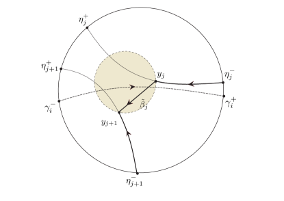
(a) non-coprime elements

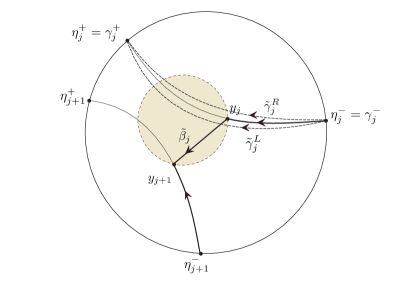
(b) Coprime elements

Figure 7. Intersection computations

Let us move to the remaining cases. The purpose of taking the “left and right perturbations” of $\tilde{\eta}_{j}$ is to take care of the situation when $\eta_{j}$ (or $\eta_{j+1}$) and $\gamma_{i}$ are not coprime. So let us assume now that $\tilde{\eta}_{j}=\tilde{\gamma}_{i}$ (the case when $\tilde{\eta}_{j+1}=\tilde{\gamma}_{i}$ is symmetric).

Then in this case assume that $\eta_{j+1}^{-}$ is on the left of $\tilde{\eta}_{j}$ and $\tilde{\gamma}_{i}$ has the same orientation as $\tilde{\eta}_{j}$ (the other cases being symmetric). It then follows that

$${\rm m}_{i,j}({\mathcal{F}}^{L})={\iota}(\tilde{\gamma}_{i},\tilde{\beta}_{j}^{L}) = 0,$$ (100)

$${\rm m}_{i,j}({\mathcal{F}}^{R})={\iota}(\tilde{\gamma}_{i},\tilde{\beta}_{j}^{R}) = 1.$$ (101)

It follows that

$$\frac{1}{2}({\rm m}_{i,j}({\mathcal{F}}^{L})+{\rm m}_{i,j}({\mathcal{F}}^{R}))=\frac{1}{2}=[\gamma_{i}^{-}\gamma_{i}^{+},\eta_{j}^{-}\eta_{j+1}^{-}].$$

We illustrate that case in Figure 7b. This finishes the proof of Equation (89).

Proof of Equation (90) and (91): The proof follows from the same ideas as the previous ones.

∎

8. Asymptotics

This section is the main computational core of this article. Our goal is to compute asymptotic product formulas, namely understand the behaviour of the special product formula when the repetition in the arcs becomes infinite. This allows us to describe the limit of certain Wilson loops as elementary functions – see Proposition 8.2.4.

The goal of this section is to obtain Corollary 8.3.2 which is an asymptotic product formula for the Goldman bracket of elementary functions.

We first need some facts about vanishing sequences

8.1. Properties of vanishing sequences

In this paragraph, we shall be given a vanishing sequence $\{\Gamma_{p}\}_{p\in\mathbb{N}}$ of finite index subgroups of $\pi_{1}(S)$. We need some notation and definition

• Let $\operatorname{gh}_{p}$ be the function defined on ${\mathsf{H}}(n,S)$ by

  $$\operatorname{gh}_{p}(\rho){}\mathrel{\mathop{:}}={}\operatorname{gh}\left(\left.\rho\right|_{\Gamma_{p}}\right).$$

• For any positive integer $p$ and primitive element $\xi$ in $\Gamma_{0}$, let $\xi(p)$ be the positive integer so that

  $$\langle\xi^{\xi(p)}\rangle=\langle\xi\rangle\cap\Gamma_{p}.$$

  We write $\xi_{p}=\xi^{\xi(p)}$ and we denote the associated closed geodesic by $\tilde{\xi}_{p}$.

Definition 8.1.1.

[$N$-nice covering] Let $\gamma$ and $\eta$ be primitive coprime elements of $\Gamma_{0}=\pi_{1}(S)$. Let $N$ be a positive integer. We say that $\Gamma_{p}$ is $N$-nice with respect to $\gamma$ and $\eta$, if the intersection loop $c_{x}(\tilde{\gamma}_{p},\tilde{\eta}_{p})$ is either trivial or satisfies

$$\pi_{p}\left(c_{x}(\tilde{\gamma}_{p},\tilde{\eta}_{p})\right)=\gamma^{k_{1}}.\eta^{-k_{2}},$$

where $k_{1}$ and $k_{2}$ satisfy

$$\gamma(p)-N>k_{1}>N\hbox{ and }\eta(p)-N>k_{2}>N.$$

We need the following properties of vanishing sequences which we summarise in the next proposition.

Proposition 8.1.2.

Let $\{\Gamma_{p}\}_{p\in\mathbb{N}}$ be a vanishing sequence of finite index subgroups of $\pi_{1}(S)$ and $\{S_{p}\}_{p\in\mathbb{N}}$ the corresponding sequence of coverings so that $\pi_{1}(S_{p})=\Gamma_{p}$. Then

1. when $p$ goes to infinity, $\operatorname{gh}_{p}$ converge uniformly to 0 on every compact of ${\mathsf{H}}(n,S)$,

2. for any primitive coprime elements $\gamma$ and $\eta$, for all $N$, there exists $p_{0}$ so that for every $p>p_{0}$, $\Gamma_{p}$ is $N$-nice with respect to $\gamma$ and $\eta$.

3. Let $G=(\gamma_{0},\ldots,\gamma_{p})$ and $F=(\eta_{0},\ldots,\eta_{q})$ be tuples of primitive elements of $\pi_{1}(S)\setminus\{1\}$ such that $(\gamma_{i},\gamma_{i+1})$ as well as $(\eta_{j},\eta_{j+1})$ are pairwise coprime. Then for $q$ large enough, $G$ and $F$ satisfy the Good Position Hypothesis 7.5.1 as elements of $\pi_{1}(S_{q})$.

8.1.1. Proof of Proposition 8.1.2

Proposition 8.1.2 will the concatenation of Propositions 8.1.3, 8.1.5 and 8.1.6 proved thereafter. Proposition 8.1.4 is an intermediate step in proving Proposition 8.1.6. We fix in this paragraph a vanishing sequence $\{\Gamma_{p}\}_{p\in\mathbb{N}}$.

Remember that we identify primitive elements in $\pi_{1}(S)$ and in any of its finite index subgroup.

Proposition 8.1.3.

When $p$ goes to infinity, $\operatorname{gh}_{p}$ converge uniformly to 0 on every compact of ${\mathsf{H}}(n,S)$.

Proof.

For all positive number $K$ and compact $C$ in $\mathsf{H}(n,S)$, let consider the following subset of $\pi_{1}(S)$

$$Z_{K}{}\mathrel{\mathop{:}}={}\left\{\gamma\in\pi_{1}(S)\setminus\{\operatorname{Id}\}\mid\exists\rho\in C,\ \ \left|\frac{\lambda_{2}(\rho(\gamma))}{\lambda_{1}(\rho(\gamma))}\right|>K\right\}.$$

By Proposition 3.3.4, the set of conjugacy classes in $Z_{K}$ is a finite set. Let $Z^{0}_{K}$ be a finite set in $\pi_{1}(S)$ of representatives of the conjugacy classes of $Z_{K}$. From the definition of vanishing sequences, it follows that there exists $p_{0}$ that that for all $p>p_{0}$, we have

$$Z^{0}_{K}\cap\Gamma_{p}=\emptyset.$$

Since $\Gamma_{p}$ is normal, it follows that

$$Z_{K}\cap\Gamma_{p}=\emptyset.$$

Then by definition, the girth of any representation in $C$ restricted to $\Gamma_{p}$ is smaller than $K$. Thus the family of functions $\operatorname{gh}_{p}$ converges uniformly to zero on $C$, when $p$ goes to $\infty$. ∎

The following proposition is well known.

Proposition 8.1.4.

Let $\gamma$ be an element of $\Gamma_{0}$. Then there exists $p_{0}$ such that for all $p>p_{0}$, the geodesics $\tilde{\gamma}_{p}$ is simple.

Proof.

Let

$$\hat{A}_{\gamma}{}\mathrel{\mathop{:}}={}\{\xi\in\Gamma_{0}\mid\xi(\tilde{\gamma})\cap\tilde{\gamma}\not=\emptyset.\}\subset\Gamma_{0}/\langle\gamma\rangle.$$

Observe that $\hat{A}_{\gamma}$ is invariant by right multiplication by $\gamma$ and that its projection in $\Gamma_{0}/\langle\gamma\rangle$ is a finite set. Thus there exists $p_{0}$ so that for every $p>p_{0}$,

$$A_{\gamma}\cap\Gamma_{p}\subset\langle\gamma\rangle.$$

This implies that the projection of $\tilde{\gamma}$ in $S_{p}$ is a simple closed geodesic, indeed the existence of a self intersection point implies the existence of an element $\xi$ in $\Gamma_{p}$ so that $\xi(\tilde{\gamma})\cap\tilde{\gamma}\not=\emptyset$. ∎

We finally need.

Proposition 8.1.5.

Let $\gamma$ and $\eta$ two coprime primitive elements of $\Gamma_{0}=\pi_{1}(S)$. Let $N$ be a positive integer.

Then there exists $p_{0}$ such that for all $p>p_{0}$, $\Gamma_{p}$ is $N$-nice with respect to $\gamma$ and $\eta$.

Proof.

We assume using the previous proposition that $\tilde{\gamma}_{p}$ and $\tilde{\eta}_{p}$ are simple.

Step 1 We shall prove the following assertion

For any $N>0$, there exists $p_{0}$ such that for any $p>p_{0}$, for any integers $k$ such that $0<k\leqslant N$ and for any $m$ then

$$\gamma^{k}\eta^{m}\not\in\Gamma_{p}\hbox{ and }\gamma^{m}\eta^{-k}\not\in\Gamma_{p}.$$

This is an immediate application of Proposition 6.2.2. Let $H{}\mathrel{\mathop{:}}={}\{\gamma^{k}\mid 0<k\leqslant N\}$. Since $\gamma$ and $\eta$ are coprime then $H\cap\langle\eta\rangle=\emptyset$. Using Proposition, 6.2.2, we get that there exists $p_{0}$ so that for all $p>p_{0}$,

$$H\cap\left(\Gamma_{p}.\langle\eta\rangle\right)=\emptyset.$$

In other words, for all $n$ and $k$ so that $0<k\leqslant N$,

$$\gamma^{k}.\eta^{n}\not\in\Gamma_{p}.$$

A symmetric argument concludes the proof.

Step 2 We now prove.

If $x\in\gamma_{p}\cap\eta_{p}$, then there exists positive integers $k_{1}$ and $k_{2}$ such that the intersection loop $c_{p}(x){}\mathrel{\mathop{:}}={}c_{x}(\tilde{\gamma}_{p},\tilde{\eta}_{p})$ satisfies

$$\pi_{p}\left(c_{p}(x)\right)=\gamma^{k_{2}}.\eta^{-k_{1}},$$

where the equality is as homotopy classes in $S_{0}=S$ We can as well assume (using the first step and a shift in $p$) that the projection of the axis of $\gamma$ and $\eta$ are simple geodesics in $S_{0}$. Let also

$$A_{p}{}\mathrel{\mathop{:}}={}\{\xi\in\Gamma_{p}\mid\xi(\tilde{\eta})\cap\tilde{\gamma}\not=\emptyset\}\subset\Gamma_{p}.$$

Observe that $A_{p}$ is invariant by left multiplication by $\gamma$ and right multiplication by $\eta$. Let $\hat{A}_{p}$ be the projection of $A_{p}$ in $\langle\eta_{p}\rangle\backslash\Gamma_{p}/\langle\eta_{p}\rangle$. Observe also that we have a bijection from $\hat{A}_{p}$ to

$$I_{p}{}\mathrel{\mathop{:}}={}\pi_{p}(\tilde{\gamma})\cap\pi_{p}(\tilde{\eta})\subset S_{p}$$

given by

$$\langle\gamma\rangle.\xi.\langle\eta\rangle\to\pi_{p}(\xi(\tilde{\eta})\cap\tilde{\gamma}).$$

In particular $\hat{A}_{p}$ is finite since $I_{p}$ is finite. Moreover, if $x$ in $I_{p}$ comes in this procedure from an element $a$ in $A_{p}$, then $a$ represents the intersection loop of $x$.

Since $\hat{A}_{0}$ is finite, using the double coset separability property, there exists $p_{0}$ such that for all $p>p_{0}$, we have

$$A_{0}\cap\Gamma_{p}\subset\langle\gamma\rangle\langle\eta\rangle,$$

Since $A_{p}\subset A_{0}\cap\Gamma_{p},$ It follows that the projection in $S_{0}$ of any intersection loop $c_{x}(\gamma_{p},\eta_{p})$ is homotopic to $\gamma^{n}.\eta^{-m}$ with $n$ and $m$ positive integers.

Conclusion of the proof The Proposition follows at once from the two steps of the proof. ∎

Proposition 8.1.6.

Let $G=(\gamma_{0},\ldots,\gamma_{p})$ and $F=(\eta_{0},\ldots,\eta_{q})$ be tuples of primitive elements of $\pi_{1}(S)\setminus\{1\}$ such that $(\gamma_{i},\gamma_{i+1})$ as well as $(\eta_{j},\eta_{j+1})$ are pairwise coprime. Then for $m$ large enough, $G$ and $F$ satisfy the Good Position Hypothesis 7.5.1 as elements of $\pi_{1}(S_{m})$.

Proof.

Let us check the four conditions of the Good Position Hypothesis. Let $G=(\gamma_{0},\ldots,\gamma_{p})$ and $F=(\eta_{0},\ldots,\eta_{q})$ be primitive elements of $\pi_{1}(S)\setminus\{1\}$ such that $(\gamma_{i},\gamma_{i+1})$ as well as $(\eta_{j},\eta_{j+1})$ are pairwise coprime.

1. Let $B\subset\tilde{S}$ be a ball containing all the intersections $\tilde{\gamma}_{i}\cap\tilde{\eta}_{j}$ when $\gamma_{i}$ and $\eta_{j}$ are coprime. Thus Condition (1) of the Good Position Hypothesis is satisfied.

2. Let

   $$F{}\mathrel{\mathop{:}}={}\{\xi\in\pi_{1}(S)\mid B\cap\xi(B)\not=\emptyset\}.$$

   The set $F$ is finite. Thus, by Proposition 6.2.2 (applied to $\gamma=\eta=\operatorname{Id}$), there exists $p_{0}$, such that for all $p>p_{0}$, we have

   $$F\cap\Gamma_{p}=\{\operatorname{Id}\}.$$

   Thus Condition (2) of the Good Position Hypothesis is satisfied.

3. Next, for every $\zeta\in\{\gamma_{0},\ldots\gamma_{p},\eta_{0},\ldots,\eta_{q}\}$ the set

   $$H_{\zeta}{}\mathrel{\mathop{:}}={}\{\xi\in\Gamma/\langle\zeta\rangle\mid\xi(\tilde{\zeta})\cap B\not=\emptyset\}.$$

   finite. Thus by Proposition 6.2.2 (applied to $\gamma=\operatorname{Id}$, $\eta=\zeta$), there exists $p_{0}$, such that for all $p>p_{0}$, we have

   $$H_{\zeta}\langle\zeta\rangle\cap\Gamma_{p}=\langle\zeta\rangle.$$

   Thus Condition (3) of the Good Position Hypothesis is satisfied.

4. Finally Condition (4) of the Good Position Hypothesis is satisfied for $p$ large enough by Proposition 8.1.4.

∎

8.2. Asymptotic product formula for Wilson loops

In all this paragraph, we shall be given a finite index subgroup $\Gamma_{k}$ of $\Gamma_{0}=\pi_{1}(S)$, corresponding to a covering $S_{k}\to S_{0}=S$. Then, if $\rho$ is a Hitchin representation of $\pi_{1}(S)$ in $\mathsf{PSL}_{n}(\mathbb{R})$, $\rho_{k}$ will denote the restriction of $\rho$ to $\Gamma_{k}$.

Let $(\gamma_{0},\ldots,\gamma_{q})$ and $(\eta_{0},\ldots,\eta_{q^{\prime}})$ be two tuples of primitive elements of $\pi_{1}(S)$. We assume that $(\gamma_{i},\gamma_{i+1})$ as well as $(\eta_{j},\eta_{j+1})$ are all pairwise coprime.

Let then $\hat{\gamma}_{i}$ and $\hat{\eta}_{i}$ be the representatives of $\gamma_{i}$ and $\eta_{i}$ in $\Gamma_{k}$, and

$${\bf F}^{(p)}=\hat{\gamma}_{1}^{p}\ldots\hat{\gamma}_{q}^{p}, {\bf G}^{(p)}=\hat{\eta}_{1}^{p}\ldots\hat{\eta}_{q^{\prime}}^{p}.$$ (102)

We want to understand the asymptotics when $p$ goes to infinity of the following function

$${B^{k}_{p}}(\gamma_{0},\ldots,\gamma_{q};\eta_{0},\ldots,\eta_{q^{\prime}}):\,\mathsf{H}(n,S_{k})\to\mathbb{R},$$

defined by

$${B^{k}_{p}}(\gamma_{0},\ldots,\gamma_{q};\eta_{0},\ldots,\eta_{q^{\prime}}){}\mathrel{\mathop{:}}={}\frac{{\mathsf{W}}(\{{\bf G}^{(p)},{\bf F}^{(p)}\}_{S_{k}})}{{{\mathsf{W}}({\bf G}^{(p)}){\mathsf{W}}({\bf F}^{(p)})}}$$ (103)

Let then

$${\rm f}_{i,j}=[\gamma_{i}^{-}\gamma_{i}^{+},\eta_{j}^{-}\eta_{j}^{+}], {\rm n}_{i,j}=[\gamma_{i}^{-}\gamma_{i+1}^{-},\eta_{j}^{-}\eta_{j}^{+}],$$ (104)

$${\rm m}_{i,j}=[\gamma_{i}^{-}\gamma_{i}^{+},\eta_{j}^{-}\eta_{j+1}^{-}], {\rm q}_{i,j}=[\gamma_{i}^{-}\gamma_{i+1}^{-},\eta_{j}^{-}\eta_{j+1}^{-}].$$ (105)

The following paragraph is devoted to the proof of the following Proposition

Proposition 8.2.1.

[Asymptotic product formula] For every compact set $U$ in ${\mathsf{H}}(n,S)$, for every positive integer $N$, for $k$ large enough, we have for every $\rho$ in $U$

$$B^{k}_{p}(\gamma_{0},\ldots,\gamma_{q},\eta_{0},\ldots,\eta_{q^{\prime}})(\rho)=\sum_{\begin{subarray}{c}0\leqslant i\leqslant q\\ 0\leqslant j\leqslant q^{\prime}\end{subarray}}\Bigg{(}(p-1)^{2}{\rm f}_{i,j}{\mathsf{T}}(\gamma_{i},\eta_{j})\\ +(p-1)\left(\frac{{\mathsf{T}}(\gamma_{i+1},\gamma_{i},\eta_{j})}{{\mathsf{T}}(\gamma_{i},\gamma_{i+1})}\left({\rm n}_{i,j}+{\rm f}_{i+1,j}\right)+\frac{{\mathsf{T}}(\gamma_{i},\eta_{j+1},\eta_{j})}{{\mathsf{T}}(\eta_{j},\eta_{j+1})}\left({\rm m}_{i,j}+{\rm f}_{i,j+1}\right)\right)\\ +\frac{{\mathsf{T}}(\gamma_{i+1},\gamma_{i},\eta_{j+1},\eta_{j})}{{\mathsf{T}}(\gamma_{i+1},\gamma_{i}){\mathsf{T}}(\eta_{j},\eta_{j+1})}\left({\rm q}_{i,j}+{\rm n}_{i,j+1}+{\rm m}_{i+1,j}+{\rm f}_{i+1,j+1}\right)\Bigg{)}\\ +p^{2}{\rm R}_{i,j}{\mathsf{T}}(\gamma_{i},\eta_{j})+K\cdotp\left(\operatorname{gh}_{k}(\rho)+\operatorname{gh}_{0}(\rho)^{N}\right),$$ (106)

where

• $K$ is bounded on $U$,

• $\operatorname{gh}_{k}(\rho)=\operatorname{gh}\left(\left.\rho\right|_{\Gamma_{k}}\right)$ where $\operatorname{gh}(\rho)$ is the girth of $\rho$ – see Definition 3.3.3.

• the integers ${\mathrm{f}}_{i,j}$, ${\mathrm{m}}_{i,j}$, ${\mathrm{n}}_{i,j}$ and ${\mathrm{q}}_{i,j}$ are defined in Equations (105) .

• ${\rm R}_{i,j}$ is an integer that only depends on $\gamma_{i}$ and $\eta_{j}$.

We will use bouquets to express this asymptotics using our product formula for bouquets.

8.2.1. Preliminary asymptotics

Let $\rho$ be a representation of $\Gamma_{0}=\pi_{1}(S)$. For any $k$, let $\rho_{k}{}\mathrel{\mathop{:}}={}\left.\rho\right|_{\Gamma_{k}}$. Let $\gamma_{0},\ldots,\gamma_{q}$ and $\eta_{0},\ldots,\eta_{q^{\prime}}$ be primitive elements of $\Gamma_{0}$ and $\widehat{\gamma}_{0},\ldots,\widehat{\gamma}_{q}$ and $\widehat{\eta}_{0},\ldots,\widehat{\eta}_{q^{\prime}}$ be the corresponding elements in $\Gamma_{k}$, so that

$$\widehat{\gamma}_{i}=\gamma_{i}^{Q_{i}}, \widehat{\eta}_{j}=\eta_{j}^{P_{j}},$$ (107)

where $Q_{i}$ and $P_{j}$ are positive integers. In this proof, $K$, $K_{0}$,$K_{1}$, …will be the generic symbol for a function of $\rho$ bounded by a continuous function that only depends on the relative position of the eigenvectors of $\rho(\gamma_{i})$ and $\rho(\eta_{i})$ and does not depend on $k$. Let us define

$$\widehat{\mathsf{g}}_{i}=\rho_{k}(\widehat{\gamma}_{i}), \widehat{\mathsf{h}}_{i}=\rho_{k}(\widehat{\eta}_{i}),$$ (108)

$${\mathsf{g}}_{i}=\rho(\gamma_{i}), {\mathsf{h}}_{i}=\rho(\eta_{i}),$$ (109)

and

$$\widehat{\mathsf{F}}_{i}^{(p,m)} {}\mathrel{\mathop{:}}={} \widehat{\mathsf{g}}_{i}^{m}\widehat{\mathsf{g}}_{i+1}^{p}\ldots\widehat{\mathsf{g}}_{i-1}^{p}\widehat{\mathsf{g}}_{i}^{p-m},$$ (110)

$$\widehat{\mathsf{G}}_{i}^{(p,m)} {}\mathrel{\mathop{:}}={} \widehat{\mathsf{h}}_{i}^{m}\widehat{\mathsf{h}}_{i+1}^{p}\ldots\widehat{\mathsf{h}}_{i-1}^{p}\widehat{\mathsf{h}}_{i}^{p-m},$$ (111)

$${\mathsf{F}}_{i}^{(p,m)} {}\mathrel{\mathop{:}}={} {\mathsf{g}}_{i}^{m}{\mathsf{g}}_{i+1}^{p}\ldots{\mathsf{g}}_{i-1}^{p}{\mathsf{g}}_{i}^{p-m},$$ (112)

$${\mathsf{G}}_{i}^{(p,m)} {}\mathrel{\mathop{:}}={} {\mathsf{h}}_{i}^{m}{\mathsf{h}}_{i+1}^{p}\ldots{\mathsf{h}}_{i-1}^{p}{\mathsf{h}}_{i}^{p-m}.$$ (113)

We prove in this paragraph two propositions

Proposition 8.2.2.

For all positive integer $p$, for all integer $m$, with $0<m<p$, we have for any $\rho$ in a compact set $U$ of ${\mathsf{H}}(n,S)$,

$$\frac{\widehat{\mathsf{F}}_{i}^{(p,0)}}{\operatorname{tr}\left(\widehat{\mathsf{F}}_{i}^{(p,0)}\right)} = \frac{\accentset{\bullet}{\mathsf{g}}_{i}\accentset{\bullet}{\mathsf{g}}_{i-1}}{\operatorname{tr}(\accentset{\bullet}{\mathsf{g}}_{i}\accentset{\bullet}{\mathsf{g}}_{i-1})}+K_{1}.\operatorname{gh}_{k}(\rho)^{p},$$ (114)

$$\frac{\widehat{\mathsf{F}}_{i}^{(p,p)}}{\operatorname{tr}\left(\widehat{\mathsf{F}}_{i}^{(p,0)}\right)} = \frac{\accentset{\bullet}{\mathsf{g}}_{i+1}\accentset{\bullet}{\mathsf{g}}_{i}}{\operatorname{tr}(\accentset{\bullet}{\mathsf{g}}_{i}\accentset{\bullet}{\mathsf{g}}_{i+1})}+K_{2}.\operatorname{gh}_{k}(\rho)^{p},$$ (115)

$$\frac{\widehat{\mathsf{F}}_{i}^{(p,m)}}{\operatorname{tr}\left(\widehat{\mathsf{F}}_{i}^{(p,0)}\right)} = \accentset{\bullet}{\mathsf{g}}_{i}+K_{3}.\operatorname{gh}_{k}(\rho)^{\inf(m,p-m)},$$ (116)

where $K_{i}$ are locally bounded functions of $\rho$.

We recall that $\accentset{\bullet}{\mathsf{g}}$ is the projector on the eigendirection of the highest eigenvalue of $\mathsf{g}$.

Proof.

Observe that for all $m$,

$$\operatorname{tr}\left(\widehat{\mathsf{F}}_{i}^{(p,m)}\right)=\operatorname{tr}\left(\widehat{\mathsf{F}}_{i}^{(p,0)}\right).$$

We use Corollary 4.1.3 and get that for all $p$,

$$\frac{\widehat{\mathsf{F}}_{i}^{(p,0)}}{\operatorname{tr}\left(\widehat{\mathsf{F}}_{i}^{(p,0)}\right)} = \frac{\accentset{\bullet}{\mathsf{g}}_{i}\accentset{\bullet}{\mathsf{g}}_{i-1}}{\operatorname{tr}(\accentset{\bullet}{\mathsf{g}}_{i}\accentset{\bullet}{\mathsf{g}}_{i-1})}+K_{3}.\operatorname{gh}_{k}(\rho)^{p},$$ (117)

$$\frac{\widehat{\mathsf{F}}_{i}^{(p,p)}}{\operatorname{tr}\left(\widehat{\mathsf{F}}_{i}^{(p,0)}\right)} = \frac{\accentset{\bullet}{\mathsf{g}}_{i+1}\accentset{\bullet}{\mathsf{g}}_{i}}{\operatorname{tr}(\accentset{\bullet}{\mathsf{g}}_{i}\accentset{\bullet}{\mathsf{g}}_{i+1})}+K_{4}.\operatorname{gh}_{k}(\rho)^{p},$$ (118)

$$\frac{\widehat{\mathsf{F}}_{i}^{(p,m)}}{\operatorname{tr}\left(\widehat{\mathsf{F}}_{i}^{(p,m)}\right)} = \accentset{\bullet}{\mathsf{g}}_{i}+K_{5}.\operatorname{gh}_{k}(\rho)^{\inf(m,p-m)},\hbox{ for }m\not\in\{0,p\}.$$ (119)

∎

We use the same notation as in the beginning of the paragraph.

Proposition 8.2.3.

Let us fix $i$ and $j$. Let

• $\{N_{1},\ldots,N_{r}\}$ be a sequence of pairwise distinct integers so that $N_{l}\geqslant N$ and $Q_{j}-N_{l}\geqslant N$.

• $\{M_{1},\ldots,M_{r}\}$ be a sequence of pairwise distinct integers so that $M_{l}\geqslant N$ and $P_{j}-M_{l}\geqslant N$.

Then, for any $\rho$ in a compact set $U$ in ${\mathsf{H}}(n,S)$, for any positive integers $p$, $m$ and $m^{\prime}$, we have

$$\sum_{1\leqslant l\leqslant r}\frac{{\mathsf{g}}_{i}^{-N_{l}}\widehat{\mathsf{F}_{i}}^{(p,m)}{\mathsf{g}}_{i}^{N_{l}}.{\mathsf{h}}_{j}^{-M_{l}}\widehat{\mathsf{G}_{j}}^{(p,m^{\prime})}{\mathsf{g}}_{i}^{M_{l}}}{\operatorname{tr}\left(\widehat{\mathsf{F}}_{i}^{(p,0)}\right)\operatorname{tr}\left(\widehat{\mathsf{G}}_{j}^{(p,0)}\right)}=r.\accentset{\bullet}{{\mathsf{g}}}_{i}\accentset{\bullet}{{\mathsf{h}}}_{j}+K\cdotp\operatorname{gh}_{0}(\rho)^{M+N}+r\operatorname{gh}_{0}(\rho)^{Np},$$ (120)

where $K$ is a locally bounded function of $\rho$ and

$$M=\inf(Q_{i}(m-1),P_{j}(m^{\prime}-1),Q_{i}p-Qm^{\prime},M_{j}p-m)\,.$$

Proof.

In this proof, as usual $K_{i}$ will denote a locally bounded function of $\rho$. For the purpose of this proof, we define

$$\widetilde{F}_{i}^{(p)}=\widehat{\mathsf{g}}_{i+1}^{p}\ldots\widehat{\mathsf{g}}_{i-1}^{p},\ \ \widetilde{G}_{j}^{(p)}=\widehat{\mathsf{h}}_{j+1}^{p}\ldots\widehat{\mathsf{h}}_{j-1}^{p}.$$

By definition, if $m\geqslant 1$, $m^{\prime}\geqslant 1$, $n<Q_{i}$ and $r<P_{j}$,

$${\mathsf{g}}_{i}^{-n}\widehat{\mathsf{F}}_{i}^{(p,m)}{\mathsf{g}}_{i}^{n} = \mathsf{g}_{i}^{Q_{i}m-n}\widetilde{\mathsf{F}}_{i}^{(p)}\mathsf{g}_{i}^{Q_{i}(p-m)+n},$$

$${\mathsf{h}}_{j}^{-r}\widehat{\mathsf{G}}_{j}^{(p,m^{\prime})}{\mathsf{h}}_{j}^{r} = \mathsf{h}_{j}^{P_{j}m^{\prime}-r}\widetilde{\mathsf{G}}_{j}^{(p)}\mathsf{h}_{i}^{P_{j}(p-m^{\prime})+r}.$$

Observe also that

$$\operatorname{tr}\left(\widehat{\mathsf{F}}_{i}^{(p,0)}\right) = \operatorname{tr}\left(\widehat{\mathsf{F}}_{i}^{(p,m)}\right),$$

$$\operatorname{tr}\left(\widehat{\mathsf{G}}_{j}^{(p,0)}\right) = \operatorname{tr}\left(\widehat{\mathsf{G}}_{j}^{(p,m^{\prime})}\right).$$

Thus using the asymptotics of Corollary 4.1.3, we get that

$$\frac{{\mathsf{g}}_{i}^{-N_{l}}\widehat{\mathsf{F}}_{i}^{(p,m)}{\mathsf{g}}_{i}^{N_{l}}}{\operatorname{tr}\left(\widehat{\mathsf{F}}_{i}^{(p,0)}\right)} = \accentset{\bullet}{\mathsf{g}}_{i}+K_{3}.\operatorname{gh}_{0}(\rho)^{R_{l}},$$

where $A_{l}=\inf(Q_{i}m-N_{l},Q_{i}(p-m)+N_{l},Np)$ and we have observed that for all $k$, $Q_{k}\geqslant N$. Similarly

$$\frac{{\mathsf{h}}_{j}^{-M_{l}}\widehat{\mathsf{G}}_{j}^{(p,m^{\prime})}{\mathsf{h}}_{i}^{M_{l}}}{\operatorname{tr}\left(\widehat{\mathsf{G}}_{j}^{(p,0)}\right)} = \accentset{\bullet}{\mathsf{h}}_{i}+K_{4}.\operatorname{gh}_{k}(\rho)^{M}.$$

where $B_{l}=\inf(P_{j}m^{\prime}-N_{l},P_{j}(p-m^{\prime})+N_{l},Np)$. Thus

$$\sum_{1\leqslant l\leqslant r}\frac{{\mathsf{g}}_{i}^{-N_{l}}\widehat{\mathsf{F}}_{i}^{(p,m)}{\mathsf{g}}_{i}^{N_{l}}.{\mathsf{h}}_{j}^{-M_{l}}\widehat{\mathsf{G}}_{j}^{(p,m^{\prime})}{\mathsf{h}}_{i}^{M_{l}}}{\operatorname{tr}\left(\widehat{\mathsf{F}}_{i}^{(p,0)}\right)\operatorname{tr}\left(\widehat{\mathsf{G}}_{j}^{(p,0)}\right)} = r\accentset{\bullet}{{\mathsf{g}}}_{i}\accentset{\bullet}{{\mathsf{h}}}_{j}+K_{0}\cdotp\left(\sum_{1\leqslant l\leqslant r}\operatorname{gh}_{0}(\rho)^{R_{l}}\right)\,,$$

where

$$R_{l}=\inf(Q_{i}m-N_{l},Q_{i}(p-m)+N_{l},P_{j}m^{\prime}-M_{l},P_{j}(p-m^{\prime})+M_{l},Np)).$$

To conclude the proof, we will show that

$$\sum_{1\leqslant l\leqslant r}\operatorname{gh}_{0}(\rho)^{R_{l}}\leqslant\frac{4\operatorname{gh}_{0}(\rho)^{N+M}}{1-\operatorname{gh}_{0}(\rho)}+r\operatorname{gh}_{0}(\rho){Np}.$$ (121)

Let

$$\mathcal{A} = \{l\mid R_{l}=Q_{i}m-N_{l}\},$$

$$\mathcal{B} = \{l\mid R_{l}=Q_{i}p-Qm+N_{l}\},$$

$$\mathcal{F} = \{l\mid R_{l}=P_{j}m^{\prime}-M_{l}\},$$

$$\mathcal{D} = \{l\mid R_{l}=P_{j}p-Pm^{\prime}+M_{l}\}.$$

By definition,

$$\sum_{l\in\mathcal{A}}\operatorname{gh}_{0}(\rho)^{R_{l}} = \sum_{l\in\mathcal{A}}\operatorname{gh}_{0}(\rho)^{Qm-N_{l}}$$

$$\leqslant \sum_{n\geqslant Q_{i}(m-1)+N}\operatorname{gh}_{0}(\rho)^{n}$$

$$\leqslant \frac{\operatorname{gh}_{0}(\rho)^{N+Q_{i}(m-1)}}{1-\operatorname{gh}_{0}(\rho)}.$$

Symmetric arguments show that

$$\sum_{i\in\mathcal{B}}\operatorname{gh}_{0}(\rho)^{R_{l}}\leqslant\frac{\operatorname{gh}_{0}(\rho)^{N+Q_{i}(p-m)}}{1-\operatorname{gh}_{0}(\rho)}\,,$$

$$\sum_{l\in\mathcal{F}}\operatorname{gh}_{0}(\rho)^{R_{l}}\leqslant\frac{\operatorname{gh}_{0}(\rho)^{N+P_{j}(m^{\prime}-1)}}{1-\operatorname{gh}_{0}(\rho)}\,,$$

$$\sum_{l\in\mathcal{D}}\operatorname{gh}_{0}(\rho)^{R_{l}}\leqslant\frac{\operatorname{gh}_{0}(\rho)^{N+P_{j}(p-m^{\prime})}}{1-\operatorname{gh}_{0}(\rho)}\,.$$

Inequality (121) – and thus the result – follows. ∎

8.2.2. Asymptotics and bouquets

We use the same notations as in the beginning of this section: Let $G=(\gamma_{0},\ldots,\gamma_{q})$ and $(F=\eta_{0},\ldots,\eta_{q^{\prime}})$ be two tuples of primitive elements of $\pi_{1}(S)$. We assume that $(\gamma_{i},\gamma_{i+1})$ as well as $(\eta_{j},\eta_{j+1})$ are all pairwise coprime. We shall use the notation of Paragraph 7.3.2.

Proposition 8.2.4.

Assume that $G$ and $F$ and $\Gamma_{k}$ satisfy the Good Position Hypothesis. Assume also that $\Gamma_{k}$ is $N$-nice for all pairs $(\gamma_{i},\eta_{j})$. Let $C$ be a bouquet in a good position representing $G$ and $F$.

Then for every compact set $U$ in ${\mathsf{H}}(n,S)$, we have for every $\rho$ in $U$,

$$B^{k}_{p}(\gamma_{0},\ldots,\gamma_{q},\eta_{0},\ldots,\eta_{q^{\prime}})(\rho)=\sum_{\begin{subarray}{c}0\leqslant i\leqslant q\\ 0\leqslant j\leqslant q^{\prime}\end{subarray}}\Bigg{(}(p-1)^{2}{\rm f}_{i,j}(\mathcal{F}){\mathsf{T}}(\gamma_{i},\eta_{j})\\ +(p-1)\left(\frac{{\mathsf{T}}(\gamma_{i+1},\gamma_{i},\eta_{j})}{{\mathsf{T}}(\gamma_{i},\gamma_{i+1})}\left({\rm n}_{i,j}(\mathcal{F})+{\rm f}_{i+1,j}(\mathcal{F})\right)+\frac{{\mathsf{T}}(\gamma_{i},\eta_{j+1},\eta_{j})}{{\mathsf{T}}(\eta_{j},\eta_{j+1})}\left({\rm m}_{i,j}(\mathcal{F})+{\rm f}_{i,j+1}(\mathcal{F})\right)\right)\\ +\frac{{\mathsf{T}}(\gamma_{i+1},\gamma_{i},\eta_{j+1},\eta_{j})}{{\mathsf{T}}(\gamma_{i+1},\gamma_{i}){\mathsf{T}}(\eta_{j},\eta_{j+1})}\left({\rm q}_{i,j}(\mathcal{F})+{\rm n}_{i,j+1}(\mathcal{F})+{\rm m}_{i+1,j}(\mathcal{F})+{\rm f}_{i+1,j+1}(\mathcal{F})\right)\Bigg{)}\\ +p^{2}\left(\sum_{i,j}I_{i,j}(1)\sharp(C_{i,j}){\mathsf{T}}(\gamma_{i},\eta_{j})\right)+K\cdotp(\operatorname{gh}_{k}(\rho)+\operatorname{gh}_{0}(\rho)^{N})\,,$$ (122)

where

• $K$ is bounded by a continuous function that only depends on the relative position of the eigenvectors of $\rho(\gamma_{i})$ and $\rho(\eta_{j})$.

• $\operatorname{gh}(\rho)$ is the girth of $\rho$ as defined in Definition 3.3.3 and $\operatorname{gh}_{k}(\rho)=\operatorname{gh}\left(\left.\rho\right|_{\Gamma_{k}}\right)$

• the integers ${\mathrm{f}}_{i,j}(\mathcal{F})$, ${\mathrm{m}}_{i,j}(\mathcal{F})$, ${\mathrm{n}}_{i,j}(\mathcal{F})$ and ${\mathrm{q}}_{i,j}(\mathcal{F})$ are defined in Equations (80).

8.2.3. Proof of Proposition 8.2.4

We now recall the Product Formula (83) that we write using the notation of Paragraph 8.2.1 as

$$B_{p}=B^{0}_{p}+\sum_{\xi\in C_{i,j}}I_{i,j}(\xi)B^{\xi}_{p},$$ (123)

where

$$B^{0}_{p} {}\mathrel{\mathop{:}}={} \frac{1}{\operatorname{tr}\left(\widehat{\mathsf{F}}^{(p,0)}\right).\operatorname{tr}\left(\widehat{\mathsf{G}}^{(p,0)}\right).}\sum_{\begin{subarray}{c}0\leqslant i\leqslant q\\ 0\leqslant j\leqslant q^{\prime}\end{subarray}}\Bigg{(}\mathop{\sum_{1\leqslant m^{\prime}\leqslant p}}_{1\leqslant m\leqslant p}{\rm f}_{i,j}(\mathcal{F})\operatorname{tr}\left(\widehat{\mathsf{F}}^{(p,m^{\prime})}_{i}\widehat{\mathsf{G}}^{(p,m)}_{j}\right)$$ (126)

$$+\mathop{\sum}_{1\leqslant m\leqslant p}{\rm m}_{i,j}(\mathcal{F})\operatorname{tr}\left(\widehat{\mathsf{F}}^{(p,m)}_{i}\widehat{\mathsf{G}}^{(p,0)}_{j}\right)$$

$$+\mathop{\sum_{1\leqslant m^{\prime}\leqslant p}}{\rm n}_{i,j}(\mathcal{F})\operatorname{tr}\left(\widehat{\mathsf{F}}^{(p,0)}_{i}\widehat{\mathsf{G}}^{(p,m^{\prime})}_{j}\right)+{\rm q}_{i,j}(\mathcal{F})\operatorname{tr}\left(\widehat{\mathsf{F}}^{(p,0)}_{i}\widehat{\mathsf{G}}^{(p,0)}_{j}\right)\Bigg{)}\,,$$

and

$$B^{\xi}_{p} {}\mathrel{\mathop{:}}={} \frac{1}{\operatorname{tr}\left(\widehat{\mathsf{F}}^{(p,0)}\right).\operatorname{tr}\left(\widehat{\mathsf{G}}^{(p,0)}\right)}\mathop{\sum_{1\leqslant m^{\prime}\leqslant p}}_{1\leqslant m\leqslant p}\operatorname{tr}\left(\widehat{\mathsf{F}}^{(p,m^{\prime})}_{i}\rho(\xi)\widehat{\mathsf{G}}^{(p,m)}_{j}\rho(\xi)^{-1}\right)\,.$$ (127)

Proposition 8.2.4 will follow from the two next propositions that treat independently the term $B^{0}_{p}$ and the term involving the $B^{\xi}_{p}$.

Proposition 8.2.5.

We have

$$B^{0}_{p}(\gamma_{0},\ldots,\gamma_{q},\eta_{0},\ldots,\eta_{q^{\prime}})=\sum_{\begin{subarray}{c}0\leqslant i\leqslant q\\ 0\leqslant j\leqslant q^{\prime}\end{subarray}}\Bigg{(}(p-1)^{2}{\rm f}_{i,j}(\mathcal{F}){\mathsf{T}}(\gamma_{i},\eta_{j})\\ +(p-1)\left(\frac{{\mathsf{T}}(\gamma_{i+1},\gamma_{i},\eta_{j})}{{\mathsf{T}}(\gamma_{i},\gamma_{i+1})}\left({\rm n}_{i,j}(\mathcal{F})+{\rm f}_{i+1,j}(\mathcal{F})\right)+\frac{{\mathsf{T}}(\gamma_{i},\eta_{j+1},\eta_{j})}{{\mathsf{T}}(\eta_{j},\eta_{j+1})}\left({\rm m}_{i,j}(\mathcal{F})+{\rm f}_{i,j+1}(\mathcal{F})\right)\right)\\ +\frac{{\mathsf{T}}(\gamma_{i+1},\gamma_{i},\eta_{j+1},\eta_{j})}{{\mathsf{T}}(\gamma_{i+1},\gamma_{i}){\mathsf{T}}(\eta_{j},\eta_{j+1})}\left({\rm q}_{i,j}(\mathcal{F})+{\rm n}_{i,j+1}(\mathcal{F})+{\rm m}_{i+1,j}(\mathcal{F})+{\rm f}_{i+1,j+1}(\mathcal{F})\right)\Bigg{)}+K\cdotp\operatorname{gh}_{k}(\rho),$$ (128)

where $K$ only depends on the position of the eigenvectors of $\rho(\gamma_{i})$ and $\rho(\eta_{j})$.

Proof.

Using the estimates for $\widehat{\mathsf{F}}_{i}^{(p,m)}$ and $\widehat{\mathsf{G}}_{i}^{(p,m)}$coming from Proposition 8.2.2 we get that

$$B^{0}_{p}=\sum_{\begin{subarray}{c}0\leqslant i\leqslant q\\ 0\leqslant j\leqslant q^{\prime}\end{subarray}}\Bigg{(}{\rm f}_{i.j}(\mathcal{F})(p-1)^{2}\operatorname{tr}(\accentset{\bullet}{\mathsf{g}}_{i}.\accentset{\bullet}{\mathsf{h}}_{j})$$ (129)

$$+ {\rm f}_{i.j}(\mathcal{F})\left(\frac{\operatorname{tr}(\accentset{\bullet}{\mathsf{g}}_{i}.\accentset{\bullet}{\mathsf{g}}_{i-1}.\accentset{\bullet}{\mathsf{h}}_{j}.\accentset{\bullet}{\mathsf{h}}_{j-1})}{\operatorname{tr}(\accentset{\bullet}{\mathsf{g}}_{i}.\accentset{\bullet}{\mathsf{g}}_{i-1})\operatorname{tr}(\accentset{\bullet}{\mathsf{h}}_{j}.\accentset{\bullet}{\mathsf{h}}_{j-1})}+(p-1)\left(\frac{\operatorname{tr}(\accentset{\bullet}{\mathsf{g}}_{i}.\accentset{\bullet}{\mathsf{h}}_{j}.\accentset{\bullet}{\mathsf{h}}_{j-1})}{\operatorname{tr}(\accentset{\bullet}{\mathsf{h}}_{j}.\accentset{\bullet}{\mathsf{h}}_{j-1})}+\frac{\operatorname{tr}(\accentset{\bullet}{\mathsf{h}}_{j}.\accentset{\bullet}{\mathsf{g}}_{i}.\accentset{\bullet}{\mathsf{g}}_{i-1})}{\operatorname{tr}(\accentset{\bullet}{\mathsf{g}}_{i}.\accentset{\bullet}{\mathsf{g}}_{i-1})}\right)\right)$$ (130)

$$+ {\rm m}_{i.j}(\mathcal{F})\left((p-1)\frac{\operatorname{tr}(\accentset{\bullet}{\mathsf{g}}_{i}.\accentset{\bullet}{\mathsf{h}}_{j+1}.\accentset{\bullet}{\mathsf{h}}_{j})}{\operatorname{tr}(\accentset{\bullet}{\mathsf{h}}_{j}.\accentset{\bullet}{\mathsf{h}}_{j+1})}+\frac{\operatorname{tr}(\accentset{\bullet}{\mathsf{g}}_{i}.\accentset{\bullet}{\mathsf{g}}_{i-1}.\accentset{\bullet}{\mathsf{h}}_{j+1}.\accentset{\bullet}{\mathsf{h}}_{j})}{\operatorname{tr}(\accentset{\bullet}{\mathsf{g}}_{i}.\accentset{\bullet}{\mathsf{g}}_{i-1})\operatorname{tr}(\accentset{\bullet}{\mathsf{h}}_{j+1}.\accentset{\bullet}{\mathsf{h}}_{j})}\right)$$ (131)

$$+ {\rm n}_{i.j}(\mathcal{F})\left((p-1)\frac{\operatorname{tr}(\accentset{\bullet}{\mathsf{g}}_{i+1}.\accentset{\bullet}{\mathsf{g}}_{i}.\accentset{\bullet}{\mathsf{h}}_{j})}{\operatorname{tr}(\accentset{\bullet}{\mathsf{g}}_{i+1}.\accentset{\bullet}{\mathsf{g}}_{i})}+\frac{\operatorname{tr}(\accentset{\bullet}{\mathsf{g}}_{i+1}.\accentset{\bullet}{\mathsf{g}}_{i}.\accentset{\bullet}{\mathsf{h}}_{j}.\accentset{\bullet}{\mathsf{h}}_{j-1})}{\operatorname{tr}(\accentset{\bullet}{\mathsf{g}}_{i}.\accentset{\bullet}{\mathsf{g}}_{i-1})\operatorname{tr}(\accentset{\bullet}{\mathsf{h}}_{j+1}.\accentset{\bullet}{\mathsf{h}}_{j})}\right)$$ (132)

$$+ {\rm q}_{i.j}(\mathcal{F})\frac{\operatorname{tr}(\accentset{\bullet}{\mathsf{g}}_{i+1}.\accentset{\bullet}{\mathsf{g}}_{i}.\accentset{\bullet}{\mathsf{h}}_{j+1}.\accentset{\bullet}{\mathsf{h}}_{j})}{\operatorname{tr}(\accentset{\bullet}{\mathsf{g}}_{i+1}.\accentset{\bullet}{\mathsf{g}}_{i})\operatorname{tr}(\accentset{\bullet}{\mathsf{h}}_{j+1}.\accentset{\bullet}{\mathsf{h}}_{j})}\Bigg{)}+K\cdotp\operatorname{gh}_{k}(\rho).$$ (133)

Using the definition of multifractions, and after reordering terms, we obtain the asymptotics of the proposition. ∎

Finally we need to understand the last term involving the sum of the terms $B^{\xi}_{p}$.

Proposition 8.2.6.

We have

$$\sum_{i,j}\sum_{\xi\in C_{i,j}}I_{i,j}(\xi)B^{\xi}_{p}=p^{2}\left(\sum_{i,j}I_{i,j}(1)\sharp(C_{i,j})\operatorname{tr}(\accentset{\bullet}{{\mathsf{g}}}_{i}\accentset{\bullet}{{\mathsf{h}}}_{j})\right)+K\cdotp\operatorname{gh}(\rho_{0})^{N},$$ (134)

where $K$ only depends on the position of the eigenvectors of $\rho(\gamma_{i})$ and $\rho(\eta_{j})$.

Proof.

We use again the notations set up in the beginning of Paragraph 8.2.1. By definition of an $N$-nice covering, any element $\xi\in C_{i,j}$ can be written as

$$\xi=\gamma_{i}^{N_{\xi}}\eta_{j}^{M_{\xi}},$$

where $N<N_{\xi}<Q_{i}-N$, and $N<M_{\xi}<P_{j}-N$. Since for $0<m<Q_{j}$, $\gamma_{i}^{m}\not\in\Gamma_{k}$, we obtain that $\xi\to N_{\xi}$ and $\xi\to M_{\xi}$ are bijections.

Moreover, since the bouquet $C$ is a lift of a bouquet $C^{0}$ in $S_{0}$, then

$$I_{i,j}(\xi)=I_{i,j}(1).$$

It follows that for any $i$ and $j$,

$$\sum_{\xi\in C_{i,j}}I_{i,j}(\xi)B^{\xi}_{p}=I_{i,j}(1)\mathop{\sum_{1\leqslant m^{\prime}\leqslant p}}_{1\leqslant m\leqslant p}\frac{\operatorname{tr}\left(B^{m,m^{\prime},i,j}_{p}\right)}{\operatorname{tr}\left(\widehat{\mathsf{F}}^{(p,0)}\right).\operatorname{tr}\left(\widehat{\mathsf{G}}^{(p,0)}\right)}\,,$$ (135)

where

$$B^{m,m^{\prime},i,j}_{p}=\sum_{\xi\in C_{i,j}}\left({\mathsf{g}}_{i}^{-N_{\xi}}\widehat{\mathsf{F}}_{i}^{(p,m)}{\mathsf{g}}_{i}^{N_{\xi}}.{\mathsf{h}}_{j}^{-M_{\xi}}\widehat{\mathsf{G}}_{j}^{(p,m^{\prime})}{\mathsf{h}}_{j}^{M_{\xi}}\right).$$

We now apply Proposition 8.2.3 to get

$$\frac{B^{m,m^{\prime},i,j}_{p}}{\operatorname{tr}\left(\widehat{\mathsf{F}}^{(p,0)}\right).\operatorname{tr}\left(\widehat{\mathsf{G}}^{(p,0)}\right)}$$ (136)

$$= I_{i,j}(1)\sharp(C_{i,j})\left(\accentset{\bullet}{{\mathsf{g}}}_{i}\accentset{\bullet}{{\mathsf{h}}}_{j}+K_{0}\operatorname{gh}_{0}(\rho)^{N+M(m,m^{\prime})}+K_{0}\operatorname{gh}_{0}(\rho)^{Np}\right),$$ (137)

where $M(m,m^{\prime})=\inf(Q_{i}(p-m),Q_{i}(m-1),P_{j}(p-m^{\prime}),P_{j}(m^{\prime}-1))$. Observe that for any $\lambda<1$

$$\mathop{\sum_{1\leqslant m^{\prime}\leqslant p}}_{1\leqslant m\leqslant p}\lambda^{M(m,m^{\prime})}\leqslant 4\sum_{n\leqslant 0}\lambda^{n}=\frac{4}{1-\lambda}.$$

Thus Equations (135) and (137) together yield

$$\sum_{i,j}\sum_{\xi\in C_{i,j}}I_{i,j}(\xi)B^{\xi}_{p}=p^{2}\left(\sum_{i,j}I_{i,j}(1)\sharp(C_{i},j).\operatorname{tr}\left(\accentset{\bullet}{{\mathsf{g}}}_{i}.\accentset{\bullet}{{\mathsf{h}}}_{j}\right)\right)+K\operatorname{gh}_{0}(\rho)^{N},$$ (138)

where we have used that $p^{2}\operatorname{gh}_{0}(\rho)^{Np}\leqslant K_{5}\operatorname{gh}_{0}(\rho)^{N}$ for some constant $K_{5}$ only depending on a compact neighborhood of $\rho$. The result finally follows from the fact that $\operatorname{tr}(\accentset{\bullet}{{\mathsf{g}}}_{i}.\accentset{\bullet}{{\mathsf{h}}}_{j})={\mathsf{T}}(\gamma_{i},\eta_{j})$. ∎

8.2.4. Proof of Proposition 8.2.1

Since $G$, $F$ and $\Gamma_{k}$ satisfy the Good Condition Hypothesis, by Proposition 7.5.2, there exist two bouquets $\mathcal{F}_{L}$ and $\mathcal{F}_{R}$ in $S$ in a homotopically good position, both representing $G$ and $F$ such that furthermore

$$\frac{1}{2}({\rm f}_{i,j}({\mathcal{F}_{L}})+{\rm f}_{i,j}(\mathcal{F}_{R})) ={\rm f}_{i,j}\,,$$

$$\frac{1}{2}({\rm n}_{i,j}(\mathcal{F}_{L})+{\rm n}_{i,j}(\mathcal{F}_{R})) ={\rm n}_{i,j}\,,$$

$$\frac{1}{2}({\rm m}_{i,j}(\mathcal{F}_{L})+{\rm m}_{i,j}(\mathcal{F}_{R})) ={\rm m}_{i,j}\,,$$

$$\frac{1}{2}({\rm q}_{i,j}(\mathcal{F}_{L})+{\rm q}_{i,j}(\mathcal{F}_{R})) ={\rm q}_{i,j}\,.$$

Thus applying Proposition 8.2.4 twice, once for $\mathcal{F}_{L}$ and once for $\mathcal{F}_{R}$, and taking the half sum, we obtain the final result.

8.3. Asymptotics of brackets of multifractions

The setting of this paragraph is the same as the previous one: we shall be given a finite index subgroup $\Gamma_{k}$ of $\Gamma_{0}=\pi_{1}(S)$, corresponding to a covering $S_{k}\to S_{0}=S$. Then, if $\rho$ is a Hitchin representation of $\pi_{1}(S)$ in $\mathsf{PSL}_{n}(\mathbb{R})$, $\rho_{k}$ will denote the restriction of $\rho$ to $\Gamma_{k}$.

Let $G=(\gamma_{0},\ldots,\gamma_{q})$ and $F=(\eta_{0},\ldots,\eta_{q^{\prime}})$ be two tuples of primitive elements of $\pi_{1}(S)$. We assume that $(\gamma_{i},\gamma_{i+1})$ as well as $(\eta_{j},\eta_{j+1})$ are all pairwise coprime. Observe that there exists $M\in\mathbb{N}$ so that for all $i$ and $j$, $\hat{\gamma}{}\mathrel{\mathop{:}}={}\gamma_{i}^{M}$ and $\hat{\eta}{}\mathrel{\mathop{:}}={}\eta_{j}^{M}$ belong to $\Gamma_{k}$ .

Then let

$$\overline{{\mathsf{W}}}_{p}(\gamma_{1},\ldots,\gamma_{q}){}\mathrel{\mathop{:}}={}\frac{{\mathsf{W}}(\hat{\gamma}_{1}^{p}\ldots\hat{\gamma}_{q}^{p})}{\prod_{i=1}^{i=q}{\mathsf{W}}(\hat{\gamma}_{i}^{p})},$$

so that

$${\mathsf{T}}=\lim_{p\to\infty}{\overline{{\mathsf{W}}}_{p}}.$$ (139)

Let now

$$A_{p}{}\mathrel{\mathop{:}}={}\frac{\{\overline{{\mathsf{W}}}_{p}(\gamma_{0},\ldots,\gamma_{q}),\overline{{\mathsf{W}}}_{p}(\eta_{0},\ldots,\eta_{q^{\prime}})\}_{S}}{\overline{{\mathsf{W}}}_{p}(\gamma_{0},\ldots,\gamma_{q}).\overline{{\mathsf{W}}}_{p}(\eta_{0},\ldots,\eta_{q^{\prime}})}$$ (140)

Let $F=(\gamma_{1},\ldots,\gamma_{q})$ and $G=(\eta_{1},\ldots,\eta_{q^{\prime}})$. We first have

Proposition 8.3.1.

We have

$$A_{p}=B_{p}(F,G)-\sum_{i}B_{p}(\gamma_{i},G)-\sum_{j}B_{p}(F,\eta_{j})+\sum_{\begin{subarray}{c}0\leqslant i\leqslant q\\ 0\leqslant j\leqslant q^{\prime}\end{subarray}}B_{p}(\gamma_{i},\eta_{j}).$$ (141)

From this proposition and Proposition 8.2.4, we will deduce the following important corollary

Corollary 8.3.2.

Assume that $G$ and $F$ and $\Gamma_{0}$ satisfy the Good Position Hypothesis. Let $k$ be a positive integer so that $\Gamma_{k}$ is $N$-nice for all pairs $(\gamma_{i},\eta_{j})$. Then

$$\frac{\left\{{\mathsf{T}}(\gamma_{0},\ldots\gamma_{q}),{\mathsf{T}}(\eta_{0},\ldots\eta_{q^{\prime}})\right\}_{S_{k}}}{{\mathsf{T}}(\gamma_{0},\ldots\gamma_{q}).{\mathsf{T}}(\eta_{0},\ldots\eta_{q^{\prime}})}$$ (142)

$$= \sum_{\begin{subarray}{c}0\leqslant i\leqslant q\\ 0\leqslant j\leqslant q^{\prime}\end{subarray}}\Big{(}\left({\rm q}_{i,j}+{\rm n}_{i,j+1}+{\rm m}_{i+1,j}+{\rm f}_{i+1,j+1}\right)\frac{{\mathsf{T}}(\gamma_{i+1}\gamma_{i},\eta_{j+1},\eta_{j})}{{\mathsf{T}}(\gamma_{i+1},\gamma_{i}){\mathsf{T}}(\eta_{j},\eta_{j+1})}$$ (145)

$$-\left({\rm n}_{i,j}+{\rm f}_{i+1,j}\right)\frac{{\mathsf{T}}(\gamma_{i+1}\gamma_{i},\eta_{j})}{{\mathsf{T}}(\gamma_{i+1},\gamma_{i})}-\left({\rm m}_{i,j}+{\rm f}_{i,j+1}\right)\frac{{\mathsf{T}}(\gamma_{i},\eta_{j+1},\eta_{j})}{{\mathsf{T}}(\eta_{j},\eta_{j+1})}$$

$$+{\rm f}_{i,j}.{\mathsf{T}}(\gamma_{i},\eta_{j})\Big{)}+K\cdotp(\operatorname{gh}_{k}(\rho)+\operatorname{gh}_{0}(\rho)^{N}),$$

where $K$ is bounded by a continuous function that only depends on the relative position of the eigenvectors of $\rho(\gamma_{i})$ and $\rho(\eta_{i})$

We first prove the corollary from the proposition, then the proposition in the next paragraph

Proof of Corollary 8.3.2: We study one by one the terms in the right hand side of the formula of Proposition 8.3.1 using the asymptotics given by Proposition 8.2.4. Let $\varepsilon=\operatorname{gh}_{k}(\rho)+\operatorname{gh}_{0}(\rho)^{N}$. First,

$$B_{p}(\gamma_{0},\ldots,\gamma_{q},\eta_{0},\ldots,\eta_{q^{\prime}})=\sum_{\begin{subarray}{c}0\leqslant i\leqslant q\\ 0\leqslant j\leqslant q^{\prime}\end{subarray}}\Bigg{(}(p^{2}{\rm R}_{i,j}+(p-1)^{2}{\rm f}_{i,j}){\mathsf{T}}(\gamma_{i},\eta_{j})\\ +(p-1)\left(\frac{{\mathsf{T}}(\gamma_{i+1},\gamma_{i},\eta_{j})}{{\mathsf{T}}(\gamma_{i},\gamma_{i+1})}\left({\rm n}_{i,j}+{\rm f}_{i+1,j}\right)+\frac{{\mathsf{T}}(\gamma_{i},\eta_{j+1},\eta_{j})}{{\mathsf{T}}(\eta_{j},\eta_{j+1})}\left({\rm m}_{i,j}+{\rm f}_{i,j+1}\right)\right)\\ +\frac{{\mathsf{T}}(\gamma_{i+1},\gamma_{i},\eta_{j+1},\eta_{j})}{{\mathsf{T}}(\gamma_{i+1},\gamma_{i}){\mathsf{T}}(\eta_{j},\eta_{j+1})}\left({\rm q}_{i,j}+{\rm n}_{i,j+1}+{\rm m}_{i+1,j}+{\rm f}_{i+1,j+1}\right)\Bigg{)}+K\varepsilon\,.$$ (146)

Let us now consider the term $B_{p}(\gamma_{i},\eta_{0},\ldots,\eta_{q^{\prime}})$. We can apply Formula (146) using the fact that in this case ${\rm q}_{i,j}={\rm n}_{i,j}=0$ to get

$$\begin{array}{c}{B}_p({\gamma }_i,{\eta }_0,\mathrm{\dots },{\eta }_{q^{\prime }})=\sum _{0⩽j⩽q^{\prime }}((p^2{\mathrm{R}}_{i,j}+{(p-1)}^2{\mathrm{f}}_{i,j})𝖳({\gamma }_i,{\eta }_j)\hfill \\ \hfill +(p-1)(𝖳({\gamma }_i,{\eta }_j)({\mathrm{f}}_{i,j}\end{array}$$

References

- [1] Michael F. Atiyah and Raoul Bott, The Yang–Mills equations over Riemann surfaces, Philos. Trans. Roy. Soc. London Ser. A 308 (1983), no. 1505, 523–615.
- [2] Marc Bourdon, Sur le birapport au bord des -espaces, Publ. Math. Inst. Hautes Études Sci. (1996), no. 83, 95–104.
- [3] Martin J. Bridgeman, The Poisson Bracket of Length functions in the Hitchin Component, arxiv preprint:1502.05975v1.
- [4] Martin J. Bridgeman, Richard Canary, François Labourie, and Andrés Sambarino, The pressure metric for Anosov representations, Geometric And Functional Analysis 25 (2015), no. 4, 1089–1179.
- [5] L. A. Dickey, Lectures on classical -algebras, Acta Applicandae Mathematicae. An International Survey Journal on Applying Mathematics and Mathematical Applications 47 (1997), no. 3, 243–321.
- [6] Vladimir Drinfel’d and V. V. Sokolov, Equations of Korteweg-de Vries type, and simple Lie algebras, Dokl. Akad. Nauk SSSR 258 (1981), no. 1, 11–16.
- [7] Vladimir V. Fock and Alexander B. Goncharov, Moduli spaces of local systems and higher Teichmüller theory, Publ. Math. Inst. Hautes Études Sci. (2006), no. 103, 1–211.
- [8] William M. Goldman, The symplectic nature of fundamental groups of surfaces, Advances in Mathematics 54 (1984), no. 2, 200–225.
- [9] by same author, Invariant functions on Lie groups and Hamiltonian flows of surface group representations, Inventiones Mathematicae 85 (1986), no. 2, 263–302.
- [10] Suresh Govindarajan, Higher-dimensional uniformisation and -geometry, Nuclear Physics. B 457 (1995), no. 1-2, 357–374.
- [11] Suresh Govindarajan and T Jayaraman, A proposal for the geometry of -gravity, Physics Letters. B 345 (1995), no. 3, 211–219.
- [12] Partha Guha, Euler–Poincaré Flows on -Opers and Integrability, Acta Applicandae Mathematicae: An International Survey … (2007).
- [13] Olivier Guichard, Composantes de Hitchin et représentations hyperconvexes de groupes de surface, Journal of Differential Geometry 80 (2008), no. 3, 391–431.
- [14] Olivier Guichard and Anna Wienhard, Anosov representations: domains of discontinuity and applications, Inventiones Mathematicae 190 (2012), no. 2, 357–438.
- [15] Nigel J Hitchin, Lie groups and Teichmüller space, Topology 31 (1992), no. 3, 449–473.
- [16] François Labourie, Anosov flows, surface groups and curves in projective space, Inventiones Mathematicae 165 (2006), no. 1, 51–114.
- [17] by same author, Cross ratios, surface groups, and diffeomorphisms of the circle, Publ. Math. Inst. Hautes Études Sci. (2007), no. 106, 139–213.
- [18] by same author, Cross ratios, Anosov representations and the energy functional on Teichmüller space, Annales Scientifiques de l’Ecole Normale Supérieure. Quatrième Série 41 (2008), no. 3, 437–469.
- [19] by same author, An algebra of observables for cross ratios, Comptes Rendus de l’Académie des Sciences. Série I. Mathématique 348 (2010), no. 9-10, 503–507.
- [20] by same authorLectures on representations of surface groups, European Mathematical Society (EMS), Zürich, (2013), Zürich Lectures in Advanced Mathematics
- [21] François Ledrappier, Structure au bord des variétés à courbure négative, vol. 13, Saint, 1995.
- [22] Franco Magri, A simple model of the integrable Hamiltonian equation, Journal of Mathematical Physics 19 (1978), no. 5, 1156–1162.
- [23] Graham Niblo, Separability properties of free groups and surface groups, J. Pure Appl. Algebra 78 (1992), no. 1, 77–84.
- [24] Jean-Pierre Otal, Le spectre marqué des longueurs des surfaces à courbure négative, Annals of Mathematics 131 (1990), no. 1, 151–162.
- [25] by same author, Sur la géometrie symplectique de l’espace des géodésiques d’une variété à courbure négative, Rev. Mat. Iberoamericana 8 (1992), no. 3, 441–456.
- [26] Andrés Sambarino, Hyperconvex representations and exponential growth, Ergodic Theory Dynam. Systems 34 (2014), no. 3, 986–1010.
- [27] by same author, Quantitative properties of convex representations, Commentarii Mathematici Helvetici 89 (2014), no. 2, 443–488.
- [28] Graeme Segal, The geometry of the KdV equation, Internat. J. Modern Phys. A 6 (1991), no. 16, 2859–2869.
- [29] Pierre van Moerbeke, Algèbres et équations non–linéaires, Astérisque (1998), no. 252, Exp. No. 839, 3, 105–129.
- [30] Edward Witten, Surprises with topological field theories, cdsweb.cern.ch.
- [31] Scott Wolpert, The Fenchel-Nielsen deformation, Annals of Mathematics 115 (1982), no. 3, 501–528.
- [32] by same author, On the Symplectic Geometry of Deformations of a Hyperbolic Surface, Annals of Mathematics 117 (1983), no. 2, 207–234.