Analysis of the 3DVAR Filter for the
Partially Observed Lorenz ’63 Model

Abstract

The problem of effectively combining data with a mathematical model constitutes a major challenge in applied mathematics. It is particular challenging for high-dimensional dynamical systems where data is received sequentially in time and the objective is to estimate the system state in an on-line fashion; this situation arises, for example, in weather forecasting. The sequential particle filter is then impractical and ad hoc filters, which employ some form of Gaussian approximation, are widely used. Prototypical of these ad hoc filters is the 3DVAR method. The goal of this paper is to analyze the 3DVAR method, using the Lorenz ’63 model to exemplify the key ideas. The situation where the data is partial and noisy is studied, and both discrete time and continuous time data streams are considered. The theory demonstrates how the widely used technique of variance inflation acts to stabilize the filter, and hence leads to asymptotic accuracy.

1 Introduction

Data assimilation concerns estimation of the state of a dynamical system by combining observed data with the underlying mathematical model. It finds widespread application in the geophysical sciences, including meteorology [15], oceanography [2] and oil reservoir simulation [24]. Both filtering methods, which update the state sequentially, and variational methods, which can use an entire time window of data, are used [1]. However, the dimensions of the systems arising in the applications of interest are enormous – of ${\cal O}(10^{9})$ in global weather forecasting, for example. This makes rigorous Bayesian approaches such as the sequential particle filter [6], for the filtering problem, or MCMC methods for the variational problem [29], prohibitively expensive in on-line scenarios.

For this reason various ad hoc methodologies are typically used. In the context of filtering these usually rely on making some form of Gaussian ansatz [32]. The 3DVAR method [18, 26] is the simplest Gaussian filter, relying on fixed (with respect to the data time-index increment) forecast and analysis model covariances, related through a Kalman update. A more sophisticated idea is to update the forecast covariance via the linearized dynamics, again computing the analysis covariance via a Kalman update, leading to the extended Kalman filter [13]. In high dimensions computing the full linearized dynamics is not practical. For this reason the ensemble Kalman filter [7, 8] is widely used, in which the forecast covariance is estimated from an ensemble of particles, and each particle is updated in Kalman fashion. An active current area of research in filtering concerns the development of methods which retain the computational expediency of approximate Gaussian filters, but which incorporate physically motivated structure into the forecast and analysis steps [22, 21], and are non-Gaussian.

Despite the widespread use of these many variants on approximate Gaussian filters, systematic mathematical analysis remains in its infancy. Because the 3DVAR method is prototypical of other more sophisticated ad hoc filters it is natural to develop a thorough understanding of the mathematical properties of this filter. Two recent papers address these issues in the context of the Navier-Stokes equation, for data streams which are discrete in time [5] and continuous in time [4]. These papers study the situation where the observations are partial (only low frequency spatial information is observed) and subject to small noise. Conditions are established under which the filter can recover from an order one initial error and, after enough time has elapsed, estimate the entire system state to within an accuracy level determined by the observational noise scale; this is termed filter accuracy. Key to understanding, and proving, these results on the 3DVAR filter for the Navier-Stokes equation are a pair of papers by Titi and co-workers which study the synchronization of the Navier-Stokes equation with a true signal which is fed into only the low frequency spatial modes of the system, without noise [25, 12]; the higher modes then synchronize because of the underlying dynamics. The idea that a finite amount of information effectively governs the large-time behaviour of the Navier-Stokes equation goes back to early studies of the equation as a dynamical system [10] and is known as the determining node or mode property in the modern literature [27]. The papers [5, 4] demonstrate that the technique of variance inflation, widely employed by practitioners in high dimensional filtering, can be understood as a method to add greater weight to the data, thereby allowing the synchronization effect to take hold.

The Lorenz ’63 model [19, 28] provides a useful metaphor for various aspects of the Navier-Stokes equation, being dissipative with a quadratic energy-conserving nonlinearity [9]. In particular, the Lorenz model exhibits a form of synchronization analogous to that mentioned above for the Navier-Stokes equation [12]. This strongly suggests that results proved for 3DVAR applied to the Navier-Stokes equation will have analogies for the Lorenz equations. The purpose of this paper is to substantiate this assertion.

The presentation is organized as follows. In section 2 we describe the Bayesian formulation of the inverse problem of sequential data assimilation; we also present a brief introduction to the relevant properties of the Lorenz ’63 model and describe the 3DVAR filtering schemes for both discrete and continuous time data streams. In section 3 we derive Theorem 3.2 concerning the 3DVAR algorithm applied to the Lorenz model with discrete time data. This is analogous to Theorem 3.3 in [5] for the Navier-Stokes equation. However, in contrast to that paper, we study Gaussian (and hence unbounded) observational noise and, as a consequence, our results are proved in mean square rather than almost surely. In section 4 we extend the accuracy result to the continuous time data stream setting: Theorem 4.1; the result is analogous to Theorem 4.3 in [4] which concerns the Navier-Stokes equation. Section 5 contains numerical results which illustrate the theory. We make concluding remarks in section 6.

2 Set-Up

In subsection 2.1 we formulate the probabilistic inverse problem which arises from attempting to estimate the state of a dynamical system subject to uncertain initial condition, and given partial, noisy observations. Subsection 2.2 introduces the Lorenz ’63 model which we employ throughout this paper. In subsections 2.3 and 2.4 we describe the discrete and continuous 3DVAR filters whose properties we study in subsequent sections.

2.1 Inverse Problem

Consider a model whose dynamics is governed by the equation

$$\frac{\textrm{d}u}{\textrm{d}t}=\mathcal{F}(u),$$ (2.1)

with initial condition $u(0)=u_{0}\in\mathbb{R}^{p}$. We assume the the initial condition is uncertain and only its statistical distribution is known, namely the Gaussian $u_{0}\sim N(m_{0},C_{0})$. Assuming that the equation has a solution for any $u_{0}\in\mathbb{R}^{p}$ and all positive times, we let $\Psi(\cdot,\cdot):\mathbb{R}^{p}\times\mathbb{R}^{+}\rightarrow\mathbb{R}^{p}$ be the solution operator for equation (2.1). Now suppose that we observe the system at equally spaced times $t_{k}=kh$ for all $k\in\mathbb{Z}^{+}$. For simplicity we write $\Psi(\cdot):=\Psi(\cdot;h).$ Defining $u_{k}=u(t_{k})=\Psi(u_{0};kh)$ we have

$$u_{k+1}=\Psi(u_{k}),\quad k\in\mathbb{Z}^{+}.$$ (2.2)

We assume that the data $\{y_{k}\}_{k\in\mathbb{Z}^{+}}$ is found from noisily observing a linear operator $H$ applied to the system state, at each time $t_{k}$, so that

$$y_{k+1}=Hu_{k+1}+{\nu}_{k+1},\quad k\in\mathbb{N}.$$ (2.3)

Here $\{\nu_{k}\}_{k\in\mathbb{N}}$ is an i.i.d. sequence of random variables, independent of $u_{0}$, with $\nu_{1}\sim N(0,\Gamma)$ and $H$ denotes a linear operator from $\mathbb{R}^{p}$ to $\mathbb{R}^{m}$, with $m\leq p.$ If the rank of $H$ is less than $p$ the system is said to be partially observed. The partially observed situation is the most commonly arising in applications and we concentrate on it here. The over-determined case $m>p$ corresponds to making more than one observation in certain directions; one approach that can be used in this situation is to average multiple observations to reduce the effective observational error variance by the square root of the number of observations in that direction, and thereby reduce to the case where the rank is less than or equal to $p$.

We denote the accumulated data up to time $k$ by $Y_{k}:={\{y_{j}\}}^{k}_{j=1}$. The pair $(u_{k},Y_{k})$ is a jointly varying random variable in $\mathbb{R}^{p}\times\mathbb{R}^{km}$. The goal of filtering is to determine the distribution of the conditioned random variable $u_{k}|Y_{k}$, and to update it sequentially as $k$ is incremented. This corresponds to a sequence of inverse problems for the system state, given observed data, and it has been regularized by means of the Bayesian formulation.

2.2 Forward Model: Lorenz ’63

When analyzing the 3DVAR approach to the filtering problem we will focus our attention on a particular model problem, namely the classical Lorenz ’63 system [19]. In this section we introduce the model and summarize the properties relevant to this paper. The Lorenz equations are a system of three coupled non-linear ordinary differential equations whose solution $u\in\mathbb{R}^{3}$, where $u=(u_{x},u_{y},u_{z})$, satisfies

$$\dot{u}_{x} = \alpha(u_{y}-u_{x}),$$ (2.4a)

$$\dot{u}_{y} = -\alpha u_{x}-u_{y}-{u_{x}}u_{z},$$ (2.4b)

$$\dot{u}_{z} = u_{x}{u_{y}}-b{u_{z}}-b(r+\alpha).$$ (2.4c)

Note that we have employed a coordinate system where origin is shifted to the point $\bigl{(}0,0,-(r+\alpha)\bigr{)}$ as discussed in [30]. Throughout this paper we will use the classical parameter values $(\alpha,b,r)=(10,\frac{8}{3},28)$ in all of our numerical experiments. At these values, the system is chaotic [31] and has one positive and one negative Lyapunov exponent and the third is zero, reflecting time translation-invariance. Our theoretical results, however, simply require that $\alpha,b>1$ and $r>0$ and we make this assumption, without further comment, throughout the remainder of the paper.

In the following it is helpful to write the Lorenz equation in the following form as given in [9],[12]:

$$\frac{du}{dt}+Au+B(u,u)=f,\quad u(0)=u_{0},$$ (2.5)

where

$$A=\left(\begin{array}[]{ccc}\alpha&-\alpha&0\\ \alpha&1&0\\ 0&0&b\end{array}\right),\quad f=\left(\begin{array}[]{c}0\\ 0\\ -b(r+\alpha)\end{array}\right)$$

$$B(u,\tilde{u})=\left(\begin{array}[]{c}0\\ (u_{x}\tilde{u_{z}}+u_{z}\tilde{u_{x}})/2\\ -(u_{x}\tilde{u_{y}}+u_{y}\tilde{u_{x}})/2\\ \end{array}\right).$$

We use the notation $\langle\cdot,\cdot\rangle$ and $|\cdot|$ for the standard Euclidean inner-product and norm. When describing our observations it will also be useful to employ the projection matrices $P$ and $Q$ defined by

$$P=\left(\begin{array}[]{ccc}1&0&0\\ 0&0&0\\ 0&0&0\end{array}\right)\quad Q=\left(\begin{array}[]{ccc}0&0&0\\ 0&1&0\\ 0&0&1\end{array}\right).$$ (2.6)

We will use the following properties of $A$ and $B$:

Properties 2.1 ([12]).

For all $u,\tilde{u}\in\mathbb{R}^{3}$

1. $\langle Au,u\rangle=\alpha u_{x}^{2}+u_{y}^{2}+bu_{z}^{2}>{|u|}^{2}$ provided that $\alpha,b>1.$

2. $\langle B(u,u),u\rangle=0$.

3. $B(u,\tilde{u})=B(\tilde{u},u)$.

4. $|B(u,\tilde{u})|\leq 2^{-1}|u||\tilde{u}|$.

5. $|\langle B(u,\tilde{u}),\tilde{u}\rangle|\leq 2^{-1}|u||\tilde{u}||P\tilde{u}|$.

We will also use the following:

Proposition 2.2.

([12], Theorem 2.2) Equation (2.5) has a global attractor $\mathcal{A}$. Let $u$ be a trajectory with $u_{0}\in\mathcal{A}$. Then $|u(t)|^{2}\leq K$ for all $t\in\mathbb{R}$ where

$$K=\frac{b^{2}(r+\alpha)^{2}}{4(b-1)}.$$ (2.7)

Figure 1 illustrates the properties of the equation. Sub-figure 1(a) shows the global attractor ${\mathcal{A}}$. Sub-figures 1(b), 1(c) and 1(d) show the components $u_{x}$, $u_{y}$ and $u_{z}$, respectively, plotted against time.

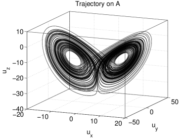
(a) Sample trajectory for a solution lying on global attractor.

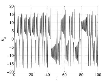
(b) $u_{x}$ component

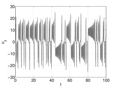
(c) $u_{y}$ component.

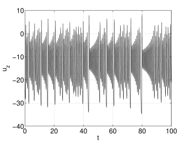
(d) $u_{z}$ component.

Figure 1: Lorenz attractor and individual components.

2.3 3DVAR: Discrete Time Data

In this section we describe the 3DVAR filtering scheme for the model (2.1) in the case where the system is observed discretely at equally spaced time points. The system state at time $t_{k}=kh$ is denoted by $u_{k}=u(t_{k})$ and the data upto that time is $Y_{k}=\{{y_{j}}\}_{j=1}^{k}.$ Recall that our aim is to find the probability distribution of $u_{k}|Y_{k}$. Approximate Gaussian filters, of which 3DVAR is a prototype, impose the following approximation:

$$\mathbb{P}(u_{k}|Y_{k})=N(m_{k},C_{k}).$$ (2.8)

Given this assumption the filtering scheme can be written as an update rule

$$(m_{k},C_{k})\mapsto(m_{k+1},C_{k+1}).$$ (2.9)

To determine this update we make a further Gaussian approximation, namely that $u_{k+1}$ given $Y_{k}$ follows a Gaussian distribution:

$$\mathbb{P}(u_{k+1}|Y_{k})=N(\hat{m}_{k+1},\hat{C}_{k+1}).$$ (2.10)

Now we can break the update rule into two steps of prediction $(m_{k},C_{k})\mapsto(\hat{m}_{k+1},\hat{C}_{k+1})$ and analysis $(\hat{m}_{k+1},\hat{C}_{k+1})\rightarrow(m_{k+1},C_{k+1})$. For the prediction step we assume that $\hat{m}_{k+1}=\Psi(m_{k})$ whilst the choice of the covariance matrix $\hat{C}_{k+1}$ depends upon the choice of particular approximate Gaussian filter under consideration. For the analysis step, (2.10) together with the fact that $y_{k+1}|u_{k+1}\sim N(Hu_{k+1},\Gamma)$ and application of Bayes’ rule, implies that

$$u_{k+1}|Y_{k+1}\sim N({m}_{k+1},{C}_{k+1})$$ (2.11)

where [11]

$$C_{k+1} = \hat{C}_{k+1}-\hat{C}_{k+1}H^{*}(\Gamma+H\hat{C}_{k+1}H^{*})^{-1}H\hat{C}_{k+1}$$ (2.12a)

$$m_{k+1} = \Psi(m_{k})+\hat{C}_{k+1}H^{*}(\Gamma+H\hat{C}_{k+1}H^{*})^{-1}\bigl{(}y_{k+1}-H\Psi({m}_{k})\bigr{)}.$$ (2.12b)

As mentioned the choice of update rule $C_{k}\rightarrow\hat{C}_{k+1}$ defines the particular approximate Gaussian filtering scheme. For the 3DVAR scheme we impose $\hat{C}_{k+1}=C\;\;\forall k\in\mathbb{N}$ where $C$ is a positive definite $p\times p$ matrix. From equation (2.12b) we then get

$$m_{k+1} = \Psi(m_{k})+CH^{*}{(\Gamma+HCH^{*})}^{-1}\bigl{(}y_{k+1}-H\Psi(m_{k})\bigr{)}$$ (2.13)

$$= (I-GH)\Psi(m_{k})+Gy_{k+1}$$

where

$$G:=CH^{*}{(\Gamma+HCH^{*})}^{-1}$$ (2.14)

is called Kalman gain matrix. The iteration (2.13) is analyzed in section 3.

Another way of defining the 3DVAR filter is by means of the following variational definition:

$$m_{k+1}=\underset{m}{\rm argmin}\;\left(\frac{1}{2}{\|C^{-\frac{1}{2}}\bigl{(}m-\Psi(m_{k})\bigr{)}\|}^{2}+\frac{1}{2}{\|\Gamma^{-\frac{1}{2}}(y_{k+1}-Hm)\|}^{2}\right).$$ (2.15)

This coincides with the previous definition because the mean of a Gaussian can be characterized as the minimizer of the negative of the logarithm of the probability density function and because the analysis step corresponds to a Bayesian Gaussian update, given the assumptions underlying the filter; indeed the fact that the negative logarithm is the sum of two squares follows from Bayes’ theorem. From the variational formulation, it is clear that the 3DVAR filter is a compromise between fitting the model and the data. The model uncertainty is characterized by a fixed covariance $C$, and the data uncertainty by a fixed covariance $\Gamma$; the ratio of the size of these two covariances will play an important role in what follows.

2.4 3DVAR: Continuous Time Data

In this section we describe the limit of high frequency observations $h\to 0$ which, with appropriate scaling of the noise covariance with respect to the observation time $h$, leads to a stochastic differential equation (SDE) limit for the 3DVAR filter. We refer to this SDE as the continuous time 3DVAR filter. We give a brief derivation, referring to [4] for further details and to [3] for a related analysis of continuous time limits in the context of the ensemble Kalman filter.

We assume the following scaling for the observation error covariance matrix: $\Gamma=\frac{1}{h}\Gamma_{0}$. Thus, although the data arrives more and more frequently, as we consider the limit $h\to 0$, it is also becoming more uncertain; this trade-off leads to the SDE limit. Define the sequence of variables $\{z_{k}\}_{k\in\mathbb{N}}$ by the relation $z_{k+1}=z_{k}+hy_{k+1}$ and $z_{0}=0$. Then

$$z_{k+1}=z_{k}+hHu_{k+1}+\sqrt{h\Gamma_{0}}\gamma_{k},\quad z_{0}=0.$$ (2.16)

Here $\gamma_{k}\sim N(0,I)$. By rearranging and taking limit as $h\rightarrow 0$ we get

$$\frac{\textrm{d}z}{\textrm{d}t}=Hu+\sqrt{\Gamma_{0}}\frac{\textrm{d}w}{\textrm{d}t},$$ (2.17)

where $w$ is an ${\mathbb{R}}^{m}$ valued standard Brownian motion. We think of $Z(t):=\{z(s)\}_{s\in[0,t]}$ as being the data. For each fixed $t$ we have the jointly varying random variable $(u(t),Z(t))\in\mathbb{R}^{p}\times C([0,t];\mathbb{R}^{m}).$ We are interested in the filtering problem of determining the sequence of conditioned probability distributions implied by the random variable $u(t)|Z(t)$ in $\mathbb{R}^{p}.$ The 3DVAR filter imposes Gaussian approximations of the form $N\bigl{(}m(t),C\bigr{)}.$ We now derive the evolution equation for $m(t).$

Recall the vector field $\mathcal{F}$ which drives equation (2.1). Using equation (2.16) in (2.13), together with the fact that $\Psi(u)=u+h\mathcal{F}(u)+{\mathcal{O}}(h^{2})$, gives

$$m_{n+1}=m_{n}+h\mathcal{F}(m_{n})+\mathcal{O}(h^{2})+hCH^{*}(\Gamma_{0}+hHCH^{*})^{-1}\left(\frac{z_{n+1}-z_{n}}{h}-Hm_{n}\right).$$ (2.18)

Rearranging and taking limit $h\rightarrow 0$ gives

$$\frac{\textrm{d}m}{\textrm{d}t}=\mathcal{F}(m)+CH^{*}\Gamma_{0}^{-1}\left(\frac{\textrm{d}z}{\textrm{d}t}-Hm\right).$$ (2.19)

Equation (2.19) defines the continuous time 3DVAR filtering scheme and is analyzed in section 4. The data should be viewed as the continuous time stream $Z(t)=\{z(s)\}_{s\in[0,t]}$ and equations (2.17) and (2.19) as stochastic differential equations driven by $w$ and $z$ respectively.

3 Analysis of Discrete Time 3DVAR

In this section we analyse the discrete time 3DVAR algorithm when applied to a partially observed Lorenz ’63 model; in particular we assume only that the $u_{x}$ component is observed. We start, in subsection 3.1, with some general discussion of error propagation properties of the filter. In subsection 3.2 we study mean square behaviour of the filter for Gaussian noise. Recall the projection matrices $P$ and $Q$ given by (2.6), we will use these in the following. We will also use $\{v_{k}\}$ to denote the exact solution sequence from the Lorenz equations which underlies the data; this is to be contrasted with $\{u_{k}\}$ which denotes the random variable which, when conditioned on the data, is approximated by the 3DVAR filter.

3.1 Preliminary Calculations

Throughout we assume that $H=(1,0,0)$, so that only $u_{x}$ is observed, and we choose the model covariance $C=\eta^{-1}\epsilon^{2}I$. We also assume that $\Gamma={\epsilon}^{2}$. The Kalman gain matrix is then $G=\frac{1}{1+\eta}H^{*}$ and the 3DVAR filter (2.13) may be written

$$m_{k+1}=\left(\frac{\eta}{1+\eta}P+Q\right)\Psi(m_{k})+\frac{1}{1+\eta}y_{k+1}H^{*}.$$ (3.1)

The scalar parameter is a design parameter whose choice we will discuss through the analysis of the iteration (3.1). Note that we are working with rather specific choices of model and observational noise covariances $C$ and $\Gamma$; we will comment on generalizations in the concluding section 6.

We define $v$ to be the true solution of the Lorenz equation (2.5) which underlies the data, and we define $v_{k}=v(kh)$, the solution at observation times. Note that, since $\Gamma={\epsilon}^{2}$, it is consistent to assume that the observation errors have the form

$$\nu_{k}=\left(\begin{array}[]{c}\epsilon\xi_{k}\\ 0\\ 0\end{array}\right),$$

where $\xi_{k}$ are i.i.d. random variables on ${\mathbb{R}}$. We will consider the case $\xi_{1}\sim N(0,1)$ for simplicity of exposition. Note that we may write

$$y_{k+1}H^{*} = Pv_{k+1}+\nu_{k+1}$$

$$= P\Psi(v_{k})+\nu_{k+1}.$$

Thus

$$m_{k+1}=\left(\frac{\eta}{1+\eta}P+Q\right)\Psi(m_{k})+\frac{1}{1+\eta}\Bigl{(}P\Psi(v_{k})+\nu_{k+1}\Bigr{)}.$$ (3.2)

Observe that

$$v_{k+1}=\Psi(v_{k})=\left(\frac{\eta}{1+\eta}P+Q\right)\Psi(v_{k})+\frac{1}{1+\eta}P\Psi(v_{k}).$$ (3.3)

We are interested in comparing $m_{k}$, the output of the filter, with $v_{k}$ the true signal which underlies the data. We define the error process $\delta(t)$ as follows:

$$\delta(t)=\left\{\begin{array}[]{c}m_{k}-v(t)\quad\textrm{if}\>\>t=t_{k}\\ \Psi(m_{k},t-t_{k})-v(t)\quad\textrm{if}\>\>t\in(t_{k},t_{k+1})\\ \end{array}\right.$$

Observe that $\delta$ is discontinuous at times $t_{j}$ which are multiples of $h$, since $m_{k+1}\neq\Psi(m_{k};h).$ In the following we write $\delta(t_{j}^{-})$ for $\lim_{t\rightarrow t_{j}^{-}}\delta(t)$ and we define $\delta_{j}=\delta(t_{j})$. Thus $\delta_{j}\neq\delta(t_{j}^{-}).$ Subtracting (3.3) from (3.2) we obtain

$$\delta(t_{k+1})=\left(\frac{\eta}{1+\eta}P+Q\right)\delta(t_{k+1}^{-})+\frac{1}{1+\eta}\nu_{k}.$$ (3.4)

Now consider the time interval $(t_{k},t_{k+1}).$ Since $\delta(t)$ is simply given by the difference of two solutions of the Lorenz equations in this interval, we have

$$\frac{d\delta}{dt}+A\delta+B(v,\delta)+B(\delta,v)+B(\delta,\delta)=0,\quad t\in(t_{k},t_{k+1}).$$ (3.5)

Taking the Euclidean inner product of equation (3.5) with $\delta$ gives

$$\frac{1}{2}\frac{d{|\delta|}^{2}}{dt}+\langle A\delta,\delta\rangle+\langle B(v,\delta),\delta\rangle+\langle B(\delta,v),\delta\rangle+\langle B(\delta,\delta),\delta\rangle=0$$ (3.6)

which, on simplifying and using Properties 2.1, gives

$$\frac{1}{2}\frac{d{|\delta|}^{2}}{dt}+\langle A\delta,\delta\rangle+2\langle B(v,\delta),\delta\rangle=0,$$ (3.7)

and hence

$$\frac{1}{2}\frac{d{|\delta|}^{2}}{dt}+{|\delta|}^{2}+2\langle B(v,\delta),\delta\rangle\leq 0.$$ (3.8)

In order to use (3.4) we wish to estimate the behaviour of $\delta(t_{k+1}^{-})$ in terms of $\delta_{k}$. The following is useful in this regard and may be proved by using (3.8) together with Properties 2.1(4). Note that $K$ is defined by equation (2.7) and is necessarily greater than or equal to one, since $b,\alpha>1.$

Proposition 3.1 ([12]).

Assume the true solution $v$ lies on the global attractor ${\mathcal{A}}$ so that ${\rm sup}_{t\geq 0}|v(t)|^{2}\leq K$ with

$$K=\frac{b^{2}(r+\alpha)^{2}}{4(b-1)}.$$

Then for $\beta=2\left(K^{1/2}-1\right)$ it follows that ${|\delta(t)|}^{2}\leq{|\delta_{k}|}^{2}e^{\beta(t-t_{k})}$ for $t\in[t_{k},t_{k+1})$.

3.2 Accuracy Theorem

In this subsection we assume that $\xi_{1}\sim N(0,1)$ and we study the behaviour of the filter in forward time when the size of the observational noise, ${\cal O}(\epsilon)$, is small. The following result shows that, provided variance inflation is employed ($\eta$ small enough), the 3DVAR filter can recover from an ${\cal O}(1)$ initial error and enter an ${\cal O}(\epsilon)$ neighbourhood of the true signal. The results are proved in mean square. The reader will observe that the bound on the error behaves poorly as the observation time $h$ goes to zero, a result of the over-weighting of observed data which is fluctuating wildly as $h\to 0.$ This effect is removed in section 4 where the observational noise is scaled appropriately, in terms of $h\to 0$, to avoid this effect.

For this theorem we define a norm $\|\cdot\|$ by $\|u\|^{2}=|u|^{2}+|Pu|^{2}$, where $|\cdot|$ is the Euclidean norm.

Theorem 3.2.

Let $v$ be a solution of the Lorenz equation (2.5) with $v(0)\in\mathcal{A}$, the global attractor. Assume that $\xi_{1}\sim N(0,1)$ so that the observational noise is Gaussian. Then there exist $h_{c}>0,\;\lambda>0$ such that for all $\eta$ sufficiently small and all $h\in(0,h_{c})$

$$\mathbb{E}{||\delta_{k+1}||}^{2}\leq(1-\lambda h)\mathbb{E}{||\delta_{k}||}^{2}+2{\epsilon}^{2}.$$ (3.9)

Consequently

$$\underset{k\rightarrow\infty}{\limsup}\,\mathbb{E}{||\delta_{k}||}^{2}\leq\frac{2{\epsilon}^{2}}{\lambda h}.$$ (3.10)

Proof.

Recall that we have $\mathbb{E}\nu_{k+1}=0$ and $\mathbb{E}{|\nu_{k+1}|}^{2}={\epsilon}^{2}$. On application of the projection $P$ to the error equation (3.4) for 3DVAR we obtain

$$\mathbb{E}{|P\delta_{k+1}|^{2}}\leq{\left(\frac{\eta}{1+\eta}\right)}^{2}\mathbb{E}{|P\delta(t_{k+1}^{-})|}^{2}+{\left(\frac{1}{1+\eta}\right)}^{2}\epsilon^{2}.\\$$ (3.11)

Since $\mathbb{E}{|Q\delta_{k+1}|^{2}}=\mathbb{E}{|Q\delta(t_{k+1}^{-})|}^{2}\leq\mathbb{E}{|\delta(t_{k+1}^{-})|}^{2}$ we also obtain the bound

$$\mathbb{E}{|\delta_{k+1}|^{2}}\leq{\left(\frac{\eta}{1+\eta}\right)}^{2}\mathbb{E}{|P\delta(t_{k+1}^{-})|}^{2}+\mathbb{E}{|\delta(t_{k+1}^{-})|}^{2}+{\left(\frac{1}{1+\eta}\right)}^{2}\epsilon^{2}.\\$$ (3.12)

Define $M_{1}$ and $M_{2}$ by

$$M_{1}(\tau)=\frac{K\alpha}{\beta+\alpha}\left(\frac{e^{\beta\tau}-e^{-\tau}}{\beta+1}-\frac{e^{-\alpha\tau}-e^{-\tau}}{1-\alpha}\right)+e^{-\tau}+2{\left(\frac{\eta}{1+\eta}\right)}^{2}\left(\frac{\alpha}{\beta+\alpha}\right)(e^{\beta\tau}-e^{-\alpha\tau})$$ (3.13)

and

$$M_{2}(\tau)=\frac{K}{1-\alpha}\left(e^{-\alpha\tau}-e^{-\tau}\right)+2{\left(\frac{\eta}{1+\eta}\right)}^{2}e^{-\alpha\tau}.$$ (3.14)

Adding (3.11) to (3.12) and using Lemma 3.3 shows that

$$\mathbb{E}{\|\delta_{k+1}\|}^{2}\leq M_{1}(h)\mathbb{E}{|\delta_{k}|}^{2}+M_{2}(h)\mathbb{E}{|P\delta_{k}|}^{2}+2{\left(\frac{1}{1+\eta}\right)}^{2}\epsilon^{2},$$ (3.15)

so that

$$\mathbb{E}{||\delta_{k+1}||}^{2}\leq M(h)\mathbb{E}{||\delta_{k}||}^{2}+\frac{2\epsilon^{2}}{(1+\eta)^{2}},$$ (3.16)

where

$$M(\tau)=\max\{M_{1}(\tau),M_{2}(\tau)\}.$$ (3.17)

Now we observe that

$$M_{1}(0)=1,\;M_{1}^{\prime}(0)=-1+2\alpha{\left(\frac{\eta}{1+\eta}\right)}^{2}\;\textrm{and}\;M_{2}(0)=2{\left(\frac{\eta}{1+\eta}\right)}^{2}.$$

Thus there exists an $h_{c}>0$ and a $\lambda>0$ such that, for all $\eta$ sufficiently small

$$M(\tau,\eta)\leq 1-\lambda\tau,\quad\forall\tau\in(0,h_{c}].$$

Hence the theorem is proved. ∎

The following lemma is used in the preceding proof.

Lemma 3.3.

Under the conditions of Theorem 3.2 for $t\in[t_{k},t_{k+1})$ we have

$${|P\delta(t)|}^{2}\leq\frac{\alpha{|\delta_{k}|}^{2}}{\beta+\alpha}\left(e^{\beta(t-t_{k})}-e^{-\alpha(t-t_{k})}\right)+{|P\delta_{k}|}^{2}e^{-\alpha(t-t_{k})}$$ (3.18)

and

$$\begin{split}|\delta(t)|^{2}\leq&\frac{K\alpha{|\delta_{k}|}^{2}}{\beta+\alpha}\left(\frac{e^{\beta(t-t_{k})}-e^{-(t-t_{k})}}{\beta+1}-\frac{e^{-\alpha(t-t_{k})}-e^{-(t-t_{k})}}{1-\alpha}\right)\\ &\quad+\frac{K{|P\delta_{k}|}^{2}}{1-\alpha}\left(e^{-\alpha(t-t_{k})}-e^{-(t-t_{k})}\right)+|\delta_{k}|^{2}e^{-(t-t_{k})}.\end{split}$$ (3.19)

Proof.

Taking inner product of (3.5) with $P\delta$, instead of with $\delta$ as previously, we get

$$\frac{1}{2}\frac{d{|P\delta|}^{2}}{dt}+\langle A\delta,P\delta\rangle=0.$$ (3.20)

Let $\delta={(\delta_{x},\delta_{y},\delta_{z})}^{T}$. Notice that ${|P\delta|}^{2}={|\delta_{x}|}^{2}$ and $\langle A\delta,P\delta\rangle=\alpha\delta_{x}^{2}-\alpha\delta_{x}\delta_{y}.$ Therefore equation (3.20) becomes

$$\frac{1}{2}\frac{d{|P\delta|}^{2}}{dt}+\alpha\delta_{x}^{2} = \alpha\delta_{x}\delta_{y}$$

$$\leq \frac{\alpha}{2}\delta_{x}^{2}+\frac{\alpha}{2}\delta_{y}^{2}$$

$$\leq \frac{\alpha}{2}\delta_{x}^{2}+\frac{\alpha}{2}{|\delta|}^{2}.$$

By rearranging and applying Proposition 3.1 we get

$$\frac{d{|P\delta|}^{2}}{dt}+\alpha{|P\delta|}^{2}\leq\alpha{|\delta(t_{k})|}^{2}e^{\beta(t-t_{k})}.$$ (3.21)

Multiplying by integrating factor $e^{\alpha(t-t_{k})}$ and integrating from $t_{k}$ to $t$ gives equation (3.18).

Analysing the non-linear term in equation (3.8) with Property 2.1(5) gives

$$|2\langle B(v,\delta),\delta\rangle| \leq |v||P\delta||\delta|$$ (3.22)

$$\leq K^{\frac{1}{2}}|P\delta||\delta|$$ (3.23)

$$\leq \frac{1}{2}K{|P\delta|}^{2}+\frac{1}{2}{|\delta|}^{2}.$$ (3.24)

Substituting (3.18) and (3.24) in (3.8) gives

$$\frac{d{|\delta|}^{2}}{dt}+{|\delta|}^{2}\leq\frac{K\alpha{|\delta_{k}|}^{2}}{\beta+\alpha}\left(e^{\beta(t-t_{k})}-e^{-\alpha(t-t_{k})}\right)+K{|P\delta_{k}|}^{2}e^{-\alpha(t-t_{k})}.$$ (3.25)

Multiplying by the integrating factor $e^{(t-t_{k})}$ and integrating from $t_{k}$ to $t$ gives

$$|\delta(t)|^{2}e^{(t-t_{k})}-|\delta_{k}|^{2}\leq\frac{K\alpha{|\delta_{k}|}^{2}}{\beta+\alpha}\left(\frac{e^{(\beta+1)(t-t_{k})}-1}{\beta+1}-\frac{e^{(1-\alpha)(t-t_{k})}-1}{1-\alpha}\right)+\frac{K{|P\delta_{k}|}^{2}}{1-\alpha}\left(e^{(1-\alpha)(t-t_{k})}-1\right).$$ (3.26)

Rearranging the above equation gives (3.19). ∎

4 Analysis of Continuous Time 3DVAR

In this section we analyse application of the 3DVAR continuous filtering algorithm for the Lorenz equation (2.5). We will use $\{v(t)\}_{t\in[0,\infty)}$ to denote the exact solution sequence from the Lorenz equations which underlies the data; this is to be contrasted with $\{u(t)\}_{t\in[0,\infty)}$ which denotes the random variable which, when conditioned on the data, is approximated by the 3DVAR filter.

We study the continuous time 3DVAR filter, again in the case where $H=(1,0,0)$, $\Gamma_{0}={\epsilon}^{2}$ and $C=\eta^{-1}{\epsilon}^{2}I$. To analyse the filter it is useful to have the truth $v$ which gives rise to the data appearing in the filter itself. Thus (2.17) gives

$$\frac{\textrm{d}z}{\textrm{d}t}=Hv+\sqrt{\Gamma_{0}}\frac{\textrm{d}w}{\textrm{d}t}.$$ (4.1)

We then eliminate $z$ in equation (2.19) by using (4.1) to obtain

$$\frac{\textrm{d}m}{\textrm{d}t}=\mathcal{F}(m)+CH^{*}\Gamma_{0}^{-1}H(v-m)+CH^{*}\Gamma_{0}^{-\frac{1}{2}}\frac{\textrm{d}w}{\textrm{d}t}.$$ (4.2)

In the specific case of the Lorenz equation we get

$$\frac{\textrm{d}m}{\textrm{d}t}=-Am-B(m,m)+f+CH^{*}\Gamma_{0}^{-1}H(v-m)+CH^{*}\Gamma_{0}^{-\frac{1}{2}}\frac{\textrm{d}w}{\textrm{d}t}.$$ (4.3)

From equation (4.2) with the choices of $C$, $H$ and $\Gamma_{0}$ detailed above we get

$$\frac{\textrm{d}m}{\textrm{d}t}=-Am-B(m,m)+f+\frac{1}{\eta}P(v-m)+\frac{\epsilon}{\eta}P\frac{\textrm{d}w}{\textrm{d}t}$$ (4.4)

where we have extended $w$ from a scalar Brownian motion to an $\mathbb{R}^{3}$-valued Brownian motion for notational convenience. This SDE has a unique global strong solution $m\in C([0,\infty);\mathbb{R}^{3})$. Indeed similar techniques used to prove the following result may be used to establish this global existence result, by applying the Itô formula to $|m|^{2}$ and using the global existence theory in [23]; we omit the details. Recall $K$ given by (2.7).

Theorem 4.1.

Let $m$ solve equation(4.4) and let $v$ solve equation (2.5) with initial data $v(0)\in{\mathcal{A}}$, the global attractor, so that $\sup_{t\geq 0}|v(t)|^{2}\leq K.$ Then for $\eta K<4$ we obtain

$$\mathbb{E}{|m(t)-v(t)|}^{2}\leq e^{-\lambda t}{|m(0)-v(0)|}^{2}+\frac{\epsilon^{2}}{\eta^{2}\lambda}(1-e^{-\lambda t}),$$ (4.5)

where $\lambda$ is defined by

$$\lambda=2\left(1-\frac{\eta K}{4}\right).$$ (4.6)

Thus

$${\rm limsup}_{t\to\infty}\mathbb{E}{|m(t)-v(t)|}^{2}\leq\frac{\epsilon^{2}}{\lambda\eta^{2}}.$$

Proof.

The true solution follows the model

$$\frac{\textrm{d}v}{\textrm{d}t}=-Av-B(v,v)+f+\frac{1}{\eta}P(v-v),$$ (4.7)

where we include the last term, which is identically zero, for clear comparison with the filter equation (4.4). Define $\delta=m-v$ and subtract equation (4.7) from equation(4.4) to obtain

$$\frac{\textrm{d}\delta}{\textrm{d}t} = -Am-B(m,m)+Av+B(v,v)-\eta^{-1}P\delta+\epsilon\eta^{-1}P\frac{\textrm{d}w}{\textrm{d}t}$$ (4.8)

$$= -A\delta-2B(v,\delta)-B(\delta,\delta)-\eta^{-1}P\delta+\epsilon\eta^{-1}P\frac{\textrm{d}w}{\textrm{d}t}.$$ (4.9)

Using Itô’s formula gives

$$\frac{1}{2}\textrm{d}{|\delta|}^{2}+\langle A\delta+2B(v,\delta)+B(\delta,\delta)+\frac{1}{\eta}P\delta,\delta\rangle{\textrm{d}t}\leq\langle\epsilon\eta^{-1}P\textrm{d}w,\delta\rangle+\frac{1}{2}\mathrm{Tr}\left(\epsilon^{2}\eta^{-2}P\right){\textrm{d}t}.$$ (4.10)

Using Lemma 4.2 and the definition of $\lambda$ gives

$$\frac{1}{2}\textrm{d}{|\delta|}^{2}+\frac{\lambda}{2}{|\delta|}^{2}{\textrm{d}t}\leq\langle\epsilon\eta^{-1}P\textrm{d}w,\delta\rangle+\frac{1}{2}\mathrm{Tr}\left(\epsilon^{2}\eta^{-2}P\right){\textrm{d}t}.$$ (4.11)

Rearranging and taking expectations gives

$$\frac{\textrm{d}\mathbb{E}{|\delta|}^{2}}{\textrm{d}t}\leq-\lambda\mathbb{E}{|\delta|}^{2}+\frac{\epsilon^{2}}{\eta^{2}}.$$ (4.12)

Use of the Gronwall inequality gives the desired result. ∎

The following lemma is used in the preceding proof.

Lemma 4.2.

Let $v\in\mathcal{A}.$ Then

$$\langle A\delta+2B(v,\delta)+B(\delta,\delta)+\frac{1}{\eta}P\delta,\delta\rangle\geq\left(1-\frac{\eta K}{4}\right){|\delta|}^{2}.$$ (4.13)

Proof.

On expanding the inner product

$$\langle A\delta+2B(v,\delta)+B(\delta,\delta)+\frac{1}{\eta}P\delta,\delta\rangle=\langle A\delta,\delta\rangle+2\langle B(v,\delta),\delta\rangle+\langle B(\delta,\delta),\delta\rangle+\langle\eta^{-1}P\delta,\delta\rangle.$$ (4.14)

We now use the Properties 2.1(1),(5) and the fact that true solution lies on the global attractor so that $|v|\leq K$. As a consequence we obtain

$$\langle A\delta+2B(v,\delta)+B(\delta,\delta)+\frac{1}{\eta}P\delta,\delta\rangle\geq{|\delta|}^{2}-K^{\frac{1}{2}}|\delta||P\delta|+\frac{1}{\eta}{|P\delta|}^{2}.$$ (4.15)

Using Young’s inequality with parameter $\theta$

$$\langle A\delta+2B(v,\delta)+B(\delta,\delta)+\frac{1}{\eta}P\delta,\delta\rangle\geq{|\delta|}^{2}-\frac{1}{2\theta}K{|P\delta|}^{2}-\frac{\theta}{2}{|\delta|}^{2}+\frac{1}{\eta}{|P\delta|}^{2}.$$ (4.16)

Taking $\theta=\frac{\eta K}{2}$ yields the desired result

$$\langle A\delta+2B(v,\delta)+B(\delta,\delta)+\frac{1}{\eta}P\delta,\delta\rangle\geq\left(1-\frac{\eta K}{4}\right){|\delta|}^{2}.$$ (4.17)

∎

5 Numerical Results

In this section we present numerical results illustrating Theorems 3.2 and 4.1 established in the two preceding sections. All experiments are conducted with the parameters $(\alpha,b,r)=(10,\frac{8}{3},28)$. Both the theorems are mean square results. However, some of our numerics are based on a single long-time realization of the filters in question, with time-averaging used in place of ensemble averaging when mean square results are displayed; we highlight when this is done.

5.1 Discrete case

Under the assumptions of Theorem 3.2 we expect the mean square error in $\delta=|v-m|$ to decrease exponentially until it is of the size of the observational noise squared. Hence we expect the estimate $m$ to converge to a neighbourhood of the true solution $v$, where the size of the neighbourhood scales as the size of the noise which pollutes in observation, in mean square. The following experiment indicates that similar behaviour is in fact observed pathwise (Figure 2), as well as in mean square over an ensemble (Figure 3). We set up the numerical experiments by computing the true solution $v$ of the Lorenz equations using the explicit Euler method, and then adding Gaussian random noise to the observed $x$-component to create the data. Throughout we fix the parameter $\eta=0.1$. In Figure 2 the observational noise $\epsilon$ is fixed and in Figure 3 we vary it over a range of scales.

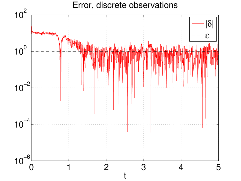
Figure 2: Decay of initial error from $\mathcal{O}(1)$ to $\mathcal{O}(\epsilon)$ for discrete observations, $\epsilon=1$, $\eta=0.1$

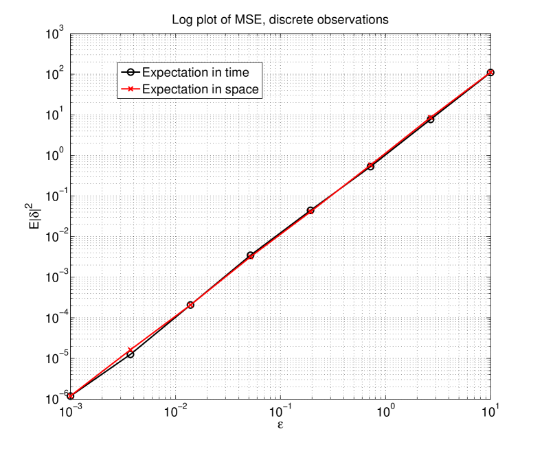
Figure 3: Log-linear dependence of asymptotic $\mathbb{E}{|\delta|^{2}}$ on $\epsilon$ for discrete observations, $\eta=0.1$.

Figure 2 concerns the behaviour of a single realization of the filter. Note that the initial error $|v(0)-m(0)|$ is around $\mathbb{E}|v|\approx 10$ and it decays exponentially with time, converging to $\mathcal{O}(\epsilon)$; for this particular case we chose $\epsilon=1.$ A consequence of the second part of Theorem 3.2 is that the logarithm of the asymptotic mean squared error $\log\mathbb{E}{|\delta|^{2}}$ varies linearly with the logarithm of the standard deviation of noise in the observations $(\epsilon)$ and this is illustrated in Figure 3. To compute the asymptotic mean square error we take two approaches. In the first, for each $\epsilon$, we time-average the error incurred within a single long trajectory of the filter. In the second approach, we consider spatial average over an ensemble of observational noises ${\nu}$, at a single time after the error has reached equilibrium. In Figure 3 we observe the log-linear decrease in the asymptotic error as the size of the noise decreases; furthermore, the slope of the graph is approximately $2$ as predicted by (3.10). Both temporal and spatial averaging deliver approximately the same slope.

5.2 Continuous case

In the case of continuous observations we again compute a true trajectory of the Lorenz equation using the explicit Euler scheme. We then simulate the SDE (4.3) using the Euler-Maruyama method. Similarly to the discrete case, we consider both pathwise and ensemble illustrations of the mean square results in Theorem 4.1. Figures 4 and 5 concern a single pathwise solution of (4.3). Recall from Theorem 4.1 that the critical value of $\eta$, beneath which the mean square theory holds, is $\eta_{c}=4/K.$ In Figure 4 we have $\eta=\frac{1}{2}\eta_{c}$ whilst in Figure 5 we have $\eta=10\eta_{c};$ in both cases the pathwise error spends most of its time at ${\cal O}(\epsilon)$, after the initial transient is removed, suggesting that the critical value of $\eta$ derived in Theorem 4.1 is not sharp. In Figure 6 we vary the size of observational error $\epsilon$ and take $\eta=\frac{1}{8}\eta_{c}.$ The initial error is expected to decay exponentially towards something of order ${\cal\epsilon}$, and this is what is observed in both the case where averaging is performed in time and in space. Indeed we observe the log-linear decrease in the asymptotic error as the size of the noise decreases, and the slope of the graph is approximately $2$, as predicted by equation (4.5).

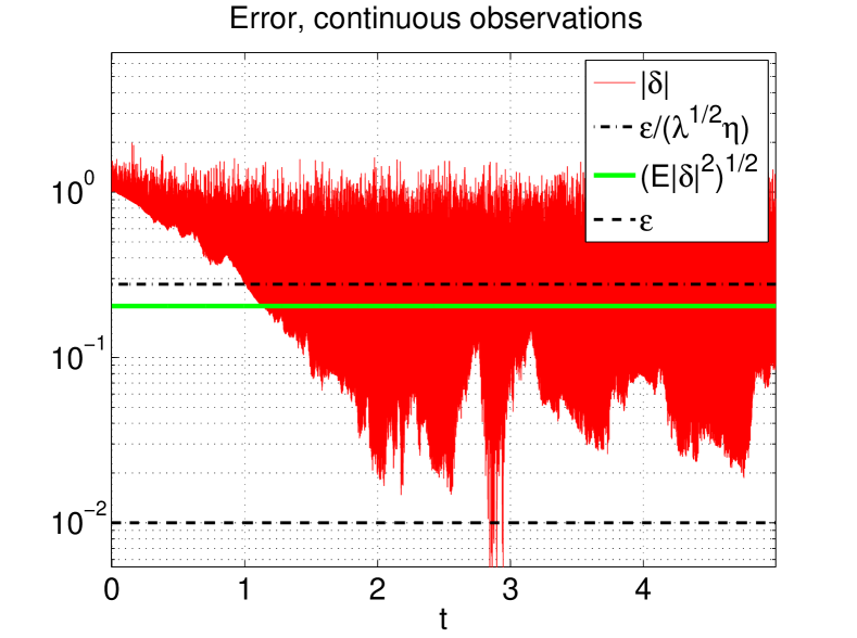
Figure 4: Decay of initial error from $\mathcal{O}(1)$ to $\mathcal{O}(\epsilon)$ for continuous observations, $\epsilon=0.01$. Results are shown for $\eta=2/K<\eta_{c}$.

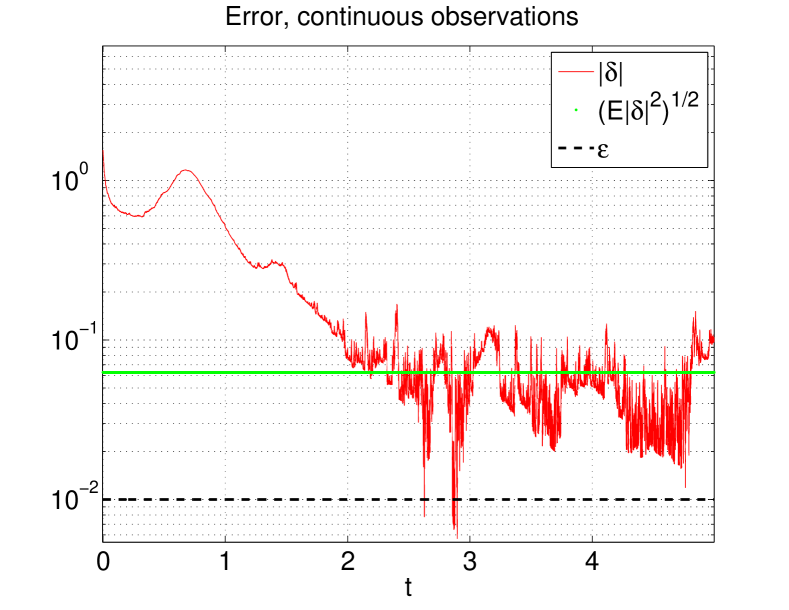
Figure 5: Decay of initial error from $\mathcal{O}(1)$ to $\mathcal{O}(\epsilon)$ for continuous observations, $\epsilon=0.01$. Results are shown for $\eta=40/K=10\eta_{c}$.

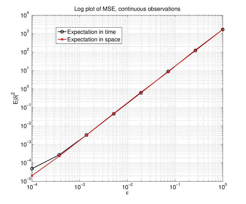
Figure 6: Log-linear dependence of asymptotic $\log\mathbb{E}{|\delta|^{2}}$ on $\log\epsilon$ for continuous observations and $\eta=1/(2K)$.

6 Conclusions

The study of approximate Gaussian filters for the incorporation of data into high dimensional dynamical systems provides a rich field for applied mathematicians. Potentially such analysis can shed light on algorithms currently in use, whilst also suggesting methods for the improvement of those algorithms. However, rigorous analysis of these filters is in its infancy. The current work demonstrates the properties of the 3DVAR algorithm when applied to the partially observed Lorenz ’63 model; it is analogous to the more involved theory developed for the 3DVAR filter applied to the partially observed Navier-Stokes equations in [5, 4]. Work of this type can be built upon in four primary directions: firstly to consider other model dynamical systems of interest to practitioners, such as the Lorenz ’96 model [20]; secondly to consider other observation models, such as pointwise velocity field measurements or Lagrangian data for the Navier-Stokes equations, building on the theory of determining modes [14]; thirdly to consider the precise relationships required between the model covariance $C$ and observation operator $H$ to ensure accuracy of the filter; and finally to consider more sophisticated filters such as the extended [13] and ensemble [7, 8] Kalman filters.

We are actively engaged in studying other models, such as Lorenz ’96, by similar techniques to those employed here; our work on Lorenz ’63 and Navier-Stokes models builds heavily on the synchronization results of Titi and coworkers and we believe that generalization of synchronization properties is a key first step in the study of other models. Regarding the second direction, Lagrangian data introduces an additional auxiliary system for the observed variables through which the system of interest is observed, necessitating careful design of correlations in the design parameters $C$, meaning that the analysis will be considerably more complicated than for Eulerian data. This links to the third direction: in general the relationship between the model covariance and observation operator required to obtain filter accuracy may be quite complicated and is an important avenue for study in this field; even for the particular Lorenz ’63 model studied herein, with observation of only the $x$ component of the system, this complexity is manifest if the covariance is not diagonal. Relating to the fourth and final direction, it is worth noting that 3DVAR is outdated operationally and empirical studies of filter accuracy have recently been focused on the more sophisticated methods such as ensemble Kalman filter and 4DVAR [16, 17]. These empirical studies indicate that the more sophisticated methods outperform 3DVAR, as expected, and therefore suggest the importance of rigorous analysis of those methods.

References

- [1] A. Apte, C. Jones, AM Stuart, and J. Voss. Data assimilation: Mathematical and statistical perspectives. International Journal for Numerical Methods in Fluids, 56(8):1033–1046, 2008.
- [2] A. Bennett. Inverse Modeling of the ocean and Atmosphere. Cambridge, 2002.
- [3] K. Bergemann and S. Reich. An ensemble kalman-bucy filter for continuous data assimilation. Meteorolog. Zeitschrift, 21:213–219, 2012.
- [4] D. Blömker, K. Law, AM Stuart, and KC Zygalakis. Accuracy and stability of the continuous-time 3dvar filter for the navier-stokes equation. arXiv preprint arXiv:1210.1594, 2012.
- [5] CEA Brett, KF Lam, KJH Law, DS McCormick, MR Scott, and AM Stuart. Accuracy and stability of filters for dissipative pdes. Physica D: Nonlinear Phenomena, 245(1):34–45, 2013.
- [6] A. Doucet, N. De Freitas, and N. Gordon. Sequential Monte Carlo methods in practice. Springer Verlag, 2001.
- [7] G. Evensen. The ensemble Kalman filter: Theoretical formulation and practical implementation. Ocean dynamics, 53(4):343–367, 2003.
- [8] G. Evensen. Data Assimilation: the Ensemble Kalman Filter. Springer Verlag, 2009.
- [9] C. Foias, M.S. Jolly, L. Kukavica, and E.S. Titi. The lorenz equationas a metaphor for the navier-stokes equation, discrete and continous dynamical systems. Discrete and Continous Dynamical Systems, 7(4):403–429, 2001.
- [10] C. Foias and G. Prodi. Sur le comportement global des solutions nonstationnaires des équations de navier-stokes en dimension 2. Rend. Sem. Mat. Univ. Padova, 39(1), 1967.
- [11] A.C. Harvey. Forecasting, Structural Time Series Models and the Kalman filter. Cambridge Univ Pr, 1991.
- [12] K. Hayden, E. Olson, and E.S. Titi. Discrete data assimilation in the lorenz and 2d navier–stokes equations. Physica D: Nonlinear Phenomena, 240(18):1416–1425, 2011.
- [13] A.H. Jazwinski. Stochastic Processes and Filtering Theory. Academic Pr, 1970.
- [14] D.A. Jones and E.S. Titi. Upper bounds on the number of determining modes, nodes, and volume elements for the navier-stokes equations. Indiana University Mathematics Journal, 42(3):875–888, 1993.
- [15] E. Kalnay. Atmospheric modeling, data assimilation, and predictability. Cambridge Univ Pr, 2003.
- [16] E. Kalnay, H. Li, T. Miyoshi, S.-C. Yang, and J. Ballabrera-Poy. 4DVAR or ensemble Kalman filter? Tellus A, 59(5):758–773, 2008.
- [17] K.J.H. Law and A.M. Stuart. Evaluating data assimilation algorithms. Monthly Weather Review, 140(11):3757–3782, 2012.
- [18] A. C. Lorenc. Analysis methods for numerical weather prediction. Quart. J. R. Met. Soc., 112(474):1177–1194, 2000.
- [19] E.N. Lorenz. Deterministic nonperiodic flow. Atmos J Sci, 20:130–141, 1963.
- [20] E.N. Lorenz. Predictability: A problem partly solved. In Proc. Seminar on Predictability, volume 1, pages 1–18, 1996.
- [21] A.J. Majda and J. Harlim. Filtering Complex Turbulent Systems. Cambridge University Press, 2012.
- [22] A.J. Majda, J. Harlim, and B. Gershgorin. Mathematical strategies for filtering turbulent dynamical systems. Discrete and Continuous Dynamical Systems - Series A, 27(2):441–486, 2010.
- [23] X. Mao. Stochastic Differential Equations And Applications. Horwood, 1997.
- [24] D.S. Oliver, A.C. Reynolds, and N. Liu. Inverse Theory for Petroleum Reservoir Characterization and History Matching. Cambridge University Press, 2008.
- [25] E. Olson and E.S. Titi. Determining modes for continuous data assimilation in 2D turbulence. Journal of statistical physics, 113(5):799–840, 2003.
- [26] D. F. Parrish and J. C. Derber. The National Meteorological Center’s spectral statistical-interpolation analysis system. Monthly Weather Review, 120(8):1747–1763, 1992.
- [27] J. C. Robinson. Infinite-Dimensional Dynamical Systems. Cambridge Texts in Applied Mathematics. Cambridge University Press, Cambridge, 2001.
- [28] C. Sparrow. The Lorenz Equations: Bifurcations, Chaos, and Strange Attractors. Springer, 1982.
- [29] A. M. Stuart. Inverse problems: a Bayesian perspective. Acta Numer., 19:451–559, 2010.
- [30] R. Temam. Infinite-Dimensional Dynamical Systems in Mechanics and Physics, volume 68 of Applied Mathematical Sciences. Springer-Verlag, New York, second edition, 1997.
- [31] W. Tucker. A rigorous ode solver and smale’s 14th problem. Journal of Foundations of Computational Mathematics, 2:53–117, 2002.
- [32] P.J. Van Leeuwen. Particle filtering in geophysical systems. Monthly Weather Review, 137:4089–4114, 2009.