Unified Field Theory and Principle of Representation Invariance

Abstract.

This article consists of two parts. The main objectives of Part 1 are to postulate a new principle of representation invariance (PRI), and to refine the unified field model of four interactions, derived using the principle of interaction dynamics (PID). Intuitively, PID takes the variation of the action functional under energy-momentum conservation constraint, and PRI requires that physical laws be independent of representations of the gauge groups. One important outcome of this unified field model is a natural duality between the interacting fields $(g,A,W^{a},S^{k})$, corresponding to graviton, photon, intermediate vector bosons $W^{\pm}$ and $Z$ and gluons, and the adjoint bosonic fields $(\Phi_{\mu},\phi^{0},\phi^{a}_{w},\phi^{k}_{s})$. This duality predicts two Higgs particles of similar mass with one due to weak interaction and the other due to strong interaction. The unified field model can be naturally decoupled to study individual interactions, leading to 1) modified Einstein equations, giving rise to a unified theory for dark matter and dark energy, 2) three levels of strong interaction potentials for quark, nucleon/hadron, and atom respectively, and 3) two weak interaction potentials. These potential/force formulas offer a clear mechanism for both quark confinement and asymptotic freedom—a longstanding problem in particle physics.

Part 2 of this article is motivated by sub-atomic decays and electron radiations, which indicate that there must be interior structures for charged leptons, quarks and mediators. The main objectives of Part 2 are 1) to propose a sub-leptons and sub-quark model, which we call weakton model, and 2) to derive a mechanism for all sub-atomic decays and bremsstrahlung. The theory is based on 1) the theory on weak and strong charges, 2) different levels of weak and strong interaction potentials, 3) a new mass generation mechanism, and 4) an angular momentum rule. The weakton model postulates that all matter particles (leptons, quarks) and mediators are made up of massless weaktons. The weakton model offers a perfect explanation for all sub-atomic decays and all generation/annihilation precesses of matter-antimatter. In particular, the precise constituents of particles involved in all decays both before and after the reaction can now be precisely derived. In addition, the bremsstrahlung phenomena can be understood using the weakton model. Also, the weakton model offers an explanation to the baryon asymmetry problem.

Introduction

There are four forces/interactions in nature: the electromagnetic force, the strong force, the weak force and the gravitational force. Classical theories describing these interactions include the Einstein general theory of relativity, the quantum electromagnetic dynamics (QED) for electromagnetism, the Weinberg-Salam electroweak theory unifying weak and electromagnetic interactions [4, 24, 22], the quantum chromodynamics (QCD) for strong interaction, and the standard model, a $U(1)\otimes SU(2)\otimes SU(3)$ gauge theory, unifying all known interactions except gravity; see among many others [10].

The main objectives of this article are three-fold. The first objective is to postulate two basic principles, which we call principle of interaction dynamics (PID) and principle of representation invariance (PRI). Intuitively, PID takes the variation of the action functional under energy-momentum conservation constraint, and was originally introduced to taking into consideration of the presence of dark energy and dark matter [15]. PRI requires that physical laws be independent of representations of the gauge groups.

The second objective is to derive a unified field theory for nature interactions, based on these two principles. The initial attempt was based solely on PID [17]. With PRI introduced in this article, we are able to substantially reduce the number of to-be-determined parameters in the unified field model to two $SU(2)$ and $SU(3)$ constant vectors $\{\alpha^{w}_{\mu}\}$ and $\{\alpha^{s}_{k}\}$, containing 11 parameters, which represent the portions distributed to the gauge potentials by the weak and strong charges $g_{w}$ and $g_{s}$.

Also, this unified field model can be naturally decoupled to study individual interactions. The second objective is to explore the duality of strong interaction based on the new field equations, derived by applying PID and PRI to a standard QCD $SU(3)$ gauge action functional. The new field equations establish a natural duality between strong gauge fields $\{S_{\mu}^{k}\}$, representing the eight gluons, and eight bosonic scalar fields. One prediction of this duality is the existence of a Higgs type bosonic spin-0 particle with mass $m\geq 100$GeV$/c^{2}$. With the duality, we derive three levels of strong interaction potentials: the quark potential $S_{q}$, the nucleon/hadron potential $S_{n}$ and the atom/molecule potential $S_{a}$. These potentials clearly demonstrates many features of strong interaction consistent with observations. In particular, these potentials offer a clear mechanisms for quark confinement, for asymptotic freedom, and for the van der Waals force. Also, in the nuclear level, the new potential is an improvement of the Yukawa potential. As the distance between two nucleons is increasing, the nuclear force corresponding to the nucleon potential $S_{n}$ behaves as repelling, then attracting, then repelling again and diminishes, consistent with experimental observations. Also, with the duality for weak interactions, we are able to derive the long overdue weak potential and force formulas.

The third objective is to derive a weakton model of elementary particles, leading to an explanation of all known sub-atomic decays and the creation/annihilation of matter/antimatter particles, as well as the baryon asymmetry problem. This objective is strongly motivated by the sub-atomic decays.

Remarkably, in the weakton model, both the spin-1 mediators (the photon, the W and Z vector bosons, and the gluons) and the spin-0 dual mediators introduced in the unified field model have the same weakton constituents, differing only by their spin arrangements. The spin arrangements clearly demonstrate that there must be dual mediators with spin-0. This observation clearly supports the unified field model presented in [17] and in Part I of this article. Conversely, the existence of the dual mediators makes the weakton constituents perfectly fit.

The unified field model appears to match Nambu’s vision. In fact, in his Nobel lecture [19], Nambu stated that

Einstein used to express dissatisfaction with his famous equation of gravity

$$G_{\mu\nu}=8\pi T_{\mu\nu}$$

His point was that, from an aesthetic point of view, the left hand side of the equation which describes the gravitational field is based on a beautiful geometrical principle, whereas the right hand side, which describes everything else, . . . looks arbitrary and ugly.

… [today] Since gauge fields are based on a beautiful geometrical principle, one may shift them to the left hand side of Einstein s equation. What is left on the right are the matter fields which act as the source for the gauge fields … Can one geometrize the matter fields and shift everything to the left?

Our understanding of his statement is that the left-hand side of the standard model is based on the gauge symmetry principle, and the right-hand side of the standard model involving the Higgs field is artificial. What Nambu presented here is a general view shared by many physicists that the Nature obeys simple beautiful laws based on a few first principles.

Both sides of our unified field model [17] and in this article are now derived from the two first principles, PID and PRI, with no Higgs field added in the Lagrangian action. The Higgs field in the standard model is now replaced by intrinsic objects, which we call the dual fields. In fact, the unified field model establishes a natural duality between the interacting fields $(g,A,W^{a},S^{k})$, corresponding to graviton, photon, intermediate vector bosons $W^{\pm}$ and $Z$ and gluons, and the dual bosonic fields $(\Phi_{\mu},\phi^{0},\phi^{a}_{w},\phi^{k}_{s})$. Here one of the three dual fields for the weak interaction $\phi^{a}_{w}$ corresponds to the Higgs field in the standard model.

The first two objectives are addressed in Part 1 of this article, and the third objective is addressed in Part 2.

Part I Field Theory

1. Introduction

This part is devoted to a field theory coupling natural interactions [15, 17]. There are several main objectives of Part 1. The first objective is to postulate a new principle of representation invariance (PRI), and to refine the unified field model, derived using the principle of interaction dynamics (PID) [17]. The unified field equations, on the one hand, are used to study the coupling mechanism of interactions in nature, and on the other hand can be decoupled to study individual interactions, leading to both experimentally verified results and new predictions. The second objective is to establish a duality theory for strong interaction, and to derive three levels of strong interaction potentials: the quark potential $S_{q}$, the nucleon/hadron potential $S_{n}$ and the atom/molecule potential $S_{a}$. These potentials clearly demonstrates many features of strong interaction consistent with observations, and offer, in particular, a clear mechanism for both quark confinement and asymptotic freedom. The third objective is to study the duality of weak interaction, and to derive such weak potential and force formula. The fourth objective is to offer our view on the structure and stability of matter, and to introduce the concept of energy levels for leptons and quarks, and for hadrons.

Hereafter we address the main motivations and ingredients of the study.

1. The original motivation is an attempt to developing gravitational field equations to provide a unified theory for dark energy and dark matter [15]. The key point is that due to the presence of dark energy and dark matter, the energy-momentum tensor of visible matter, $T_{ij}$, is no longer conserved. Namely,

$$\nabla^{i}T_{ij}\not=0,$$

where $\nabla^{i}$ is the contra-variant derivative. Since the Euler-Lagrangian of the scalar curvature part of the Einstein-Hilbert functional is conserved (Bianchi identity), it can only be balanced by the conserved part of $T_{ij}$. Thanks to an orthogonal decomposition of tensor fields into conserved and gradient parts [15], the new gravitational field equations are given then by

(1.1) $$R_{ij}-\frac{1}{2}g_{ij}R=-\frac{8\pi G}{c^{4}}T_{ij}-\nabla_{i}\nabla_{j}\varphi,$$

where $\varphi:M\to\mathbb{R}$ is a scalar function defined on the space-time manifold, whose energy density $\Phi=g^{ij}\nabla_{i}\nabla_{j}\varphi$ is conserved with mean zero:

(1.2) $$\int_{M}\Phi\sqrt{-g}dx=0.$$

Equivalently, (1.1) is the Euler-Lagrangian of the Einstein-Hilbert functional $L_{EH}$ with energy-momentum conservation constraints:

(1.3) $$(\delta L_{EH},X)=0\qquad\text{ for }X=\{X_{ij}\}\text{ with }\nabla^{i}X_{ij}=0.$$

As we have discussed in [15], the above gravitational field equations offer a unified theory for dark energy and dark matter, agreeable with all the general features/observations for both dark matter and dark energy.

2. The constraint Lagrangian action (1.3) leads us to postulate a general principle, which we call principle of interaction dynamics (PID), for deriving unified field equations coupling interactions in nature. Namely, for physical interactions with the Lagrangian action $L(g,A,\psi)$, the field equations are the Euler-Lagrangian of $L(g,A,\psi)$ with ${\rm div}_{A}$-free constraint:

(1.4) $$(\delta F(u_{0}),X)=\int_{M}\delta F(u_{0})\cdot X\sqrt{-g}dx=0\quad\text{ for }X\text{ with }{\rm div}_{A}X=0.$$

Here $A$ is a set of vector fields representing gauge and mass potentials, $\psi$ are the wave functions of particles, and div_A is defined by (2.1). It is clear that div_A-free constraint is equivalent to energy-momentum conservation.

3. We then derive in [17] the unified field equations coupling four interactions based on 1) the Einstein principle of general relativity (or Lorentz invariance) and the principle of equivalence, 2) the principle of gauge invariance, and 3) the PID. Naturally, the Lagrangian action functional is the combination of the Einstein-Hilbert action for gravity, the action of the $U(1)$ gauge field for electromagnetism, the standard $SU(2)$ Yang-Mills gauge action for the weak interactions, and the standard $SU(3)$ gauge action for the strong interactions. The unified model gives rise to a new mechanism for spontaneous gauge-symmetry breaking and for energy and mass generations with similar outcomes as the classical Higgs mechanism. One important outcome of the unified field equations is a natural duality between the interacting fields $(g,A,W^{a},S^{k})$, corresponding to graviton, photon, intermediate vector bosons $W^{\pm}$ and $Z$ and gluons, and the adjoint fields $(\Phi_{\mu},\phi^{0},\phi^{a}_{w},\phi^{k}_{s})$, which are all bosonic fields. The interaction of the bosonic particle field $\Phi$ and graviton leads to a unified theory of dark matter and dark energy and explains the acceleration of expanding universe.

4. It is classical that the electromagnetism is described by a $U(1)$ gauge field, the weak interactions are described by three $SU(2)$ gauge fields, and the strong interactions are described by eight $SU(3)$ gauge fields. In the same spirit as the Einstein principle of general relativity, physical laws should be independent of different representations of these Lie groups. Hence it is natural for us to postulate a general principle, which we call the principle of representation invariance (PRI):

Principle of Representation Invariance (PRI). All $SU(N)$ gauge theories are invariant under general linear group $GL(\mathbb{C}^{N^{2}-1})$ transformations for generators of different representations of $SU(N)$. Namely, the actions of the gauge fields are invariant and the corresponding gauge field equations are covariant under the transformations.

5. The mathematical foundation of PRI is achieved by deriving a few mathematical results for representations of the Lie group $SU(N)$. In particular, for the Lie group $SU(N)$, generators of different representations transform under general linear group $GL(\mathbb{C}^{N^{2}-1})$. We show that the structural constants $\lambda^{c}_{ab}$ of the generators of different representations should transfer as $(1,2)$-tensors. Consequently, we can construct an important $(0,2)$ $SU(N)$-tensor:

(1.5) $$G_{ab}=\frac{1}{4N}\lambda^{c}_{ad}\lambda^{d}_{cb},$$

which can be regarded as a Riemannian metric on the Lie group $SU(N)$.

Then for a set of $SU(N)$ $(N\geq 2)$ gauge fields with $N^{2}-1$ vector fields $A^{a}_{\mu}$ and $N$ spinor fields $\psi^{j}$, the following action functional is a unique functional which obeys the Lorentz invariance, the gauge invariance of the transformation (3.13), and is invariant under $GL(\mathbb{C}^{N^{2}-1})$ transformations (3.16) for generators of different representations of $SU(N)$:

(1.6) $$L_{G}=\int\left\{G_{ab}g^{\mu\alpha}g^{\nu\beta}F^{a}_{\mu\nu}F^{b}_{\alpha\beta}+\bar{\Psi}\left[i\gamma^{\mu}(\partial_{\mu}+igA^{a}_{\mu}\tau_{a})-m\right]\Psi\right\}dx.$$

Here

$$F^{a}_{\mu\nu}=\partial_{\mu}A^{a}_{\nu}-\partial_{\nu}A^{a}_{\mu}+g\lambda^{abc}A^{b}_{\mu}A^{c}_{\nu}.$$

6. It is very interesting that the unified field equations derived in [17] obey the PRI. In fact, with PRI, we are able to substantially reduce the to-be-determined parameters in our unified model to two $SU(2)$ and $SU(3)$ constant vectors

$$\{\alpha^{w}_{\mu}\}=(\alpha_{1}^{w},\alpha^{w}_{2},\alpha^{w}_{3}),\qquad\{\alpha^{s}_{k}\}=(\alpha_{1}^{s},\cdots,\alpha^{s}_{8}),$$

containing 11 parameters as given in (4.31), representing the portions distributed to the gauge potentials by the weak and strong charges. Hence they are physically needed.

It appears that any field model with the classical Higgs scalar fields added to the action functional violates PRI, and hence can only be considered as an approximation for describing the related interactions. In fact, as far as we know, the unified field model introduced in [17] and refined in this article is the only model which obeys PRI. The main reason is that our model is derived from first principles, and the spontaneous gauge-symmetry breaking as well as the mechanism of mass generation and energy creation are natural outcomes of the constraint Lagrangian action (PID).

7. In the unified model, the coupling is achieved through PID in a transparent fashion, and consequently it can be easily decoupled. In other words, both PID and PRI can be applied directly to single interactions. For gravity, for example, we have derived modified Einstein equations, leading to a unified theory for dark matter and dark energy [15].

8. New gauge field equations for strong interaction, decoupled from the unified model, are derived by applying PID to the standard $SU(3)$ gauge action functional in QCD. The new model leads to consistent results as the classical QCD, and, more importantly, to a number of new results and predictions. In particular, this model gives rise to a natural duality between the $SU(3)$ gauge fields $S_{\mu}^{k}$ ($k=1,\cdots,8$), representing the gluons, and the adjoint scalar fields $\{\phi^{k}_{s}\}$, representing Higgs type of bosonic spin-0 particles.

9. One prediction from the duality from strong interaction is the existence of a Higgs type bosonic spin-0 particle with mass $m\geq 100$GeV$/c^{2}$. It is hoped that careful examination of the LHC data may verify the existence of this Higgs type of particle due to strong interaction.

10. For the first time, we derive three levels of strong interaction potentials: the quark potential $S_{q}$, the nucleon potential $S_{n}$ and the atom/molecule potential $S_{a}$. They are given as follows:

(1.7) $$S_{q}=g_{s}\left[\frac{1}{r}-\frac{Bk^{2}_{0}}{\rho_{0}}e^{-k_{0}r}\varphi(r)\right],$$

(1.8) $$S_{n}=3\left(\frac{\rho_{0}}{\rho_{1}}\right)^{3}g_{s}\left[\frac{1}{r}-\frac{B_{n}k^{2}_{1}}{\rho_{1}}e^{-k_{1}r}\varphi(r)\right],$$

(1.9) $$S_{a}=3N\left(\frac{\rho_{0}}{\rho_{1}}\right)^{3}\left(\frac{\rho_{1}}{\rho_{2}}\right)^{3}g_{s}\left[\frac{1}{r}-\frac{B_{n}k^{2}_{1}}{\rho_{2}}e^{-k_{1}r}\varphi(r)\right],$$

where $\varphi(r)\sim{r}/{2}$, $g_{s}$ is the strong charge, $B,B_{n}$ are constants, $k_{0}=mc/\hbar$, $k_{1}=m_{\pi}c/\hbar$, $m$ is mass of the above mentioned strong interaction Higgs particle, $m_{\pi}$ is the mass of the Yukawa meson, $\rho_{0}$ is the effective quark radius, $\rho_{1}$ is the radius of a nucleon, $\rho_{2}$ is the radius of an atom/molecule, and $N$ is the number of nucleons in an atom/molecule. These potentials match very well with experimental data, and offer a number of physical conclusions. Hereafter we shall explore a few important implications of these potentials.

11. With these strong interaction potentials, the binding energy of quarks can be estimated as

(1.10) $${E_{q}}\sim\left(\frac{\rho_{1}}{\rho_{0}}\right)^{4}{E_{n}}\sim 10^{20}E_{n},$$

where $E_{n}$ is the binding energy of nucleons. Consequently, if the quark radius is considered as $\rho_{0}\sim 10^{-21}$cm, then the Planck energy level $10^{19}$ GeV is required to break a quark free. Hence these potential formulas offer a clear mechanism for quark confinement.

12. With the quark potential, there is a radius $\bar{r}$, as shown in Figure 6.1, such that two quarks closer than $\bar{r}$ are repelling, and for $r$ near $\bar{r}$, the strong interaction diminishes. Hence this clearly explains asymptotic freedom.

13. In the nucleon level, the new potential is an improvement of the Yukawa potential. The corresponding Yukawa force is always attractive. However, as the distance between two nucleons is increasing, the nucleon force corresponding to the nucleon potential $S_{n}$ behaves as repelling, then attracting, then repelling again and diminishes. This is exactly the picture that the observation tells us. In addition, these potentials give rise an estimate on the ratio between the gravitational and the strong interaction forces. This estimate indicates that near the radius of an atom, the strong repelling force is stronger than the gravitational force, and beyond the molecule radius, the strong repelling force is smaller than the gravitational force. We believe that it is this competition between the gravitational and the strong forces in the level of atoms/molecules gives rise to the mechanism of the van der Waals force.

14. The factor $\left(\frac{\rho_{0}}{\rho_{1}}\right)^{3}\left(\frac{\rho_{1}}{\rho_{2}}\right)^{3}$ in (1.9) indicates the strong interaction is of short-range, in agreement with observations. In particular, beyond molecular level, strong interaction diminishes. In addition, the derivation of these potentials clearly suggests that exchanging gluons leads to repelling force, and exchanging $\pi$-mesons (Higgs) leads to attracting force.

15. The new field equations for weak interaction, decoupled from the unified field model, provide a natural duality between weak gauge fields $\{W_{\mu}^{a}\}$, representing the $W^{\pm}$ and $Z$ intermediate vector bosons, and three bosonic scalar fields $\phi^{a}$. A possible duality is the degenerate case where the three scalar fields $\phi^{a}$ are a constant vector $\zeta_{a}$ times a single scalar field $\phi$, and the duality reduces to the duality between $\{W^{a}_{\mu}\}$ and one neutral Higgs boson field $\phi$.

16. One key point of the study is that the field equations must satisfy PRI, which induces an important $SU(2)$ constant vector $\{\alpha^{w}_{a}\}$. The components of this vector represent the portions distributed to the gauge potentials $W_{\mu}^{a}$ by the weak charge $g_{w}$. Consequently, in the same spirit as electromagnetism, the time-components $W^{a}_{0}$ of the gauge potentials represent the weak-charge potentials, and the total force exerted on a particle with $N$ weak charges $Ng_{w}$ is

(1.11) $$F_{WE}=-Ng_{w}\alpha^{w}_{a}\nabla W^{a}_{0}.$$

It is the weak charge distribution vector $\alpha^{w}_{a}$, due to PRI, that allows us to formulate the total weak potential/force as a field exerted on a particle. It is clear that $F_{WE}$ is a representation invariant scalar, obeying PRI. This clearly overcomes one of the main difficulties encountered in classical theories.

In the same token, the spatial components $\vec{W}^{a}=(W^{a}_{1},W^{a}_{2},W^{a}_{3})$ represent the weak-rotation potentials, yielding the following total weak-rotation force

(1.12) $$F_{WM}=g_{w}\varepsilon^{abc}\alpha_{a}^{w}\vec{J}^{b}\times\text{ curl}\vec{W}^{c},$$

where $\{\vec{J}^{b}\}=\{J^{b}_{1},J^{b}_{2},J^{b}_{3}\}$ is the weak charge current density, and $\varepsilon^{abc}$ is the structural constants using the Pauli matrices as generators for $SU(2)$. Also, $F_{WM}$ is a representation invariant scalar, obeying PRI.

17. With the above physical meaning of the gauge potentials and the associated forces, for the first time, we derive the weak potential and weak force formula given by

(1.13) $$W=g_{w}e^{-k_{1}r}\left[\frac{1}{r}-e^{-k_{0}r}\psi(r)\right],$$

$$F=g_{w}^{2}e^{-k_{1}r}\left[\frac{k_{1}}{r}+\frac{1}{r^{2}}-(K_{1}\psi-\psi^{\prime})e^{-k_{0}r}\right],$$

where $K_{1}=k_{0}+k_{1}$, $k_{0}=m_{H}c/\hbar$, $k_{1}=m_{W}c/\hbar$, $m_{H}$ and $m_{W}$ are the masses of the Higgs and $W$ bosons, and $\psi(r)=\psi_{1}(r)+\psi_{2}(r)\ln r$ with $\psi_{i}(r)$ being polynomials; see (9.46). This force formula is consistent with observations: there is a radius $r_{0}>0$ such that $F$ is repelling for $r<r_{0}$, and attractive for $r_{0}<r<r_{1}$. In addition, $F$ is a short-range force. Namely, $F$ diminishes for $r\geq 10^{-16}cm.$

18. With the duality, our analysis shows that the charged gauge bosons $W^{\pm}$ do not appear simultaneously with the neutral boson $Z$ in one physical situation. The same non-existence holds true for the neutral and charged Higgs particles as well.

19. The new duality model for weak interaction not only produces consistent physical conclusions as the classical GWS electroweak theory, but also leads to new insights and predictions for weak interaction. Here are a few similarities and distinctions between these two models:

• Both theories produces the right intermediate vector bosons $W^{\pm}$ and $Z$, the neutral Higgs, the neutral current, and the scaling relation, consistent with experimental observations.

• The GWS model mixes transformations of different representations of $U(1)$ and $SU(2)$, and utilizes both the electromagnetic gauge potential and the weak gauge potentials to define the intermediate vector bosons. This gauge mixing causes the decoupling of the model to electromagnetic and weak components difficult, if not impossible. This mixing also violates PRI. The duality model used in this paper can be easily decoupled to study individual interactions involved, and satisfies PRI.

• In the GWS model, the Higgs mechanism of mass generation and energy creation is achieved by introducing the Higgs sector with a Higgs scalar field in the Lagrangian action functional. The mass generation and energy creation mechanism is achieved in a completely different and much simpler fashion in the duality model by using energy-momentum conservation constraint variation (PID) to the standard $SU(2)$ gauge functional.

• Due partially to mixing the gauge fields for electromagnetic and weak interactions, it is difficult to use the classical theory to derive any force/potential formulas for weak interaction. However, as mentioned earlier, the new duality model leads naturally to a long overdue force formula for weak interaction.

20. With both weak and strong charge potentials at our disposal, for the first time, we are able to introduce energy levels of leptons and quarks using $W_{\mu}$, and energy levels for hadrons using $S_{\mu}$. Then the standard conversion of the Dirac equation for a matter field leads to the following formulation of energy levels

(1.14) $$-\nabla^{2}\Phi^{w}+\frac{g_{w}}{\hbar c}W_{0}(x)\Phi^{w}=\lambda^{w}\Phi^{w} \text{for a lepton or a quark},$$

(1.15) $$-\nabla^{2}\Phi^{H}+\frac{g_{s}}{\hbar c}S_{0}(x)\Phi^{H}=\lambda^{H}\Phi^{H} \text{for a hadron}.$$

We conclude then that each lepton or quark is represented by an eigenstate of (1.14) with corresponding eigenvalue being its binding energy, and the eigenstate of (1.14) with the lowest energy level represents the electron. Also, each hadron is represented by an eigenstate of (1.15) with the corresponding eigenvalue being its binding energy, and the eigenstate of (1.15) with the lowest energy level represents the proton.

21. A common feature of these force/charge potentials is that all four forces can be either repelling or attracting with different spatial scales. This is the essence of the stability of matter in the universe from the smallest elementary particles to largest galaxies in the universe.

Part I of this paper is organized as follows. Section 2 recapitulates PID and its motivations. Section 3 introduces PRI, and the unified field models are refined in Section 4. Section 5 addresses the duality theory for different interactions. Sections 6 and 7 derive the strong interaction potentials and their implications. Section 8 addresses various features of the duality model for weak interaction. Section 9 derives the weak potential and force formulas, and Section 10 is devoted to the comparison between the classical GWS and the new electroweak theory. Section 11 recapitulates the weak and strong potentials, and Section 12 introduces energy levels of elementary particles. Section 13 offers our view on structure and stability of matter. Brief conclusions are given in Section 14. Part 1 of this paper combines an early version of this article with [13, 14, 16].

2. Motivations for Principle of Interaction Dynamics (PID)

2.1. Recapitulation of PID

We first recall the principle of interaction dynamics (PID) proposed in [17]. Let $(M,g_{ij})$ be the 4-dimensional space-time Riemannian manifold with $\{g_{ij}\}$ the Minkowski type Riemannian metric. For an $(r,s)$-tensor $u$ we define the $A$-gradient and $A$-divergence operators $\nabla_{A}$ and ${\rm div}_{A}$ as

(2.1) $$\nabla_{A}u=\nabla u+u\otimes A,$$

$$\text{\rm div}_{A}u={\rm div}u-A\cdot u,$$

where $A$ is a vector or co-vector field, $\nabla$ and div are the usual gradient and divergent covariant differential operators.

Let $F=F(u)$ be a functional of a tensor field $u$. A tensor $u_{0}$ is called an extremum point of $F$ with the div_A-free constraint, if

(2.2) $$\frac{d}{d\lambda}F(u_{0}+\lambda X)\Big{|}_{\lambda=0}=\int_{M}\delta F(u_{0})\cdot X\sqrt{-g}dx=0\quad\forall{\rm div}_{A}X=0.$$

We now state PID, first introduced by the authors in [17].

Principle of Interaction Dynamics (PID). For all physical interactions there are Lagrangian actions

(2.3) $$L(g,A,\psi)=\int_{M}\mathcal{L}(g_{ij},A,\psi)\sqrt{-g}dx,$$

where $g=\{g_{ij}\}$ is the Riemann metric representing the gravitational potential, $A$ is a set of vector fields representing gauge and mass potentials, and $\psi$ are the wave functions of particles. The action (2.3) satisfy the invariance of general relativity (or Lorentz invariance), the gauge invariance, and PID. Moreover, the states $(g,A,\psi)$ are the extremum points of (2.3) with the ${\rm div}_{A}$-free constraint (2.2).

The following theorem is crucial for applications of PID.

Theorem 2.1 (Ma and Wang [15, 17]).

Let $F=F(g_{ij},A)$ be a functional of Riemannian metric $\{g_{ij}\}$ and vector fields $A^{1},\cdots,A^{N}$. For the ${\rm div}_{A}$-free constraint variations of $F$, we have the following assertions:

1. There is a vector field $\Phi\in H^{1}(TM)$ such that the extremum points $\{g_{ij}\}$ of $F$ with the ${\rm div}_{A}$-free constraint satisfy the equations

   (2.4) $$\frac{\delta}{\delta g_{ij}}F(g_{ij})=\left(\nabla_{i}+\sum\limits^{N}_{k=1}\alpha_{k}A^{k}_{i}\right)\Phi_{j}$$

   where $\alpha_{k}$ $(1\leq k\leq N)$ are parameters, $\nabla_{i}\Phi_{j}=\partial_{i}\Phi_{j}-\Gamma^{l}_{ij}\Phi_{l}$ are the covariant derivatives, and ${\rm div}_{A}X={\rm div}X-\sum\limits^{N}_{k=1}\alpha_{k}A^{k}\cdot X$.

2. If the first Betti number of $M$ is zero, and $A^{k}=0$ $(1\leq k\leq N)$ in (2.4), then there exists a scalar field $\varphi$ such that $\Phi=\nabla\varphi$, i.e. equations (2.4) become

   (2.5) $$\frac{\delta}{\delta g_{ij}}F(g_{ij})=-\nabla_{i}\nabla_{j}\varphi.$$

3. For each $A^{a}$, there is a scalar function $\varphi^{a}\in H^{1}(M)$ such that the extremum points $A^{a}$ of $F$ with the ${\rm div}_{A}$-free constraint satisfy the equations

   (2.6) $$\frac{\delta}{\delta A^{a}_{\mu}}F(A^{a})=(\nabla_{\mu}+\beta^{a}_{b}A^{b}_{\mu})\varphi^{a}$$

   where $\beta^{a}_{b}$ are parameters, ${\rm div}_{A}X^{a}={\rm div}X^{a}-\beta^{a}_{b}A^{b}_{\mu}X^{a}_{\mu}$ for the $a$-th vector field $X^{a}$.

Based on PID and Theorem 2.1, the field equations with respect to the action (2.3) are given in the form

(2.7) $$\frac{\delta}{\delta g_{\mu\nu}}L(g,A,\psi)=(\nabla_{\mu}+\alpha_{b}A^{b}_{\mu})\Phi_{\nu},$$

(2.8) $$\frac{\delta}{\delta A^{a}_{\mu}}L(g,A,\psi)=(\nabla_{\mu}+\beta^{a}_{b}A^{b}_{\mu})\varphi^{a},$$

(2.9) $$\frac{\delta}{\delta\psi}L(g,A,\psi)=0,$$

where $A^{k}_{\mu}=(A^{k}_{0},A^{k}_{1},A^{k}_{2},A^{k}_{3})$ $(1\leq k\leq N,N=12)$ are the gauge vector fields for the electromagnetic, weak, and strong interactions, $\Phi_{\mu}=(\Phi_{0},\Phi_{1},\Phi_{2},\Phi_{3})$ is a vector field induced by gravitational interaction, $\varphi^{a}$ are scalar fields generated from the gauge field $A^{a}$, and $\alpha_{b},\beta_{b}$ $(1\leq b\leq N)$ are coupling parameters.

Consider the action (2.3) as the natural combination of the four actions

$$\mathcal{L}=\mathcal{L}_{HE}+\mathcal{L}_{QED}+\mathcal{L}_{W}+\mathcal{L}_{QCD},$$

where $\mathcal{L}_{HE}$ is the Einstein-Hilbert action, $\mathcal{L}_{QED}$ is the QED gauge action, $\mathcal{L}_{W}$ is the $SU(2)$ gauge actions for weak interactions, and $\mathcal{L}_{QCD}$ is the action for the quantum chromodynamics. Then (2.7)-(2.9) provide the unified field equations coupling all interactions. Moreover, we see from (2.7)-(2.9) that there are too many coupling parameters need to be determined. Fortunately, this problem can be satisfactorily resolved, leading also the discovery of PRI.

In the remaining parts of this sections, we shall give some evidences and motivations for PID.

2.2. Dark matter and dark energy

The presence of dark matter and dark energy provides a strong support for PID. In this case, the energy-momentum tensor $T_{ij}$ of normal matter is no longer conserved:

$$\nabla^{i}(T_{ij})\neq 0.$$

Then as mentioned in the Introduction and in [17], the gravitational field equations (1.1) are uniquely determined by constraint Lagrangian variation, i.e. by PID. Also, by (1.2), the added term $\nabla_{i}\nabla_{j}\varphi$ has no variational structure. I other words, the term $\Phi=g^{ij}\nabla_{i}\nabla_{j}\varphi$ cannot be added into the Einstein-Hilbert functional.

2.3. Higgs mechanism and mass generation

Higgs mechanism is another main motivation to postulate PID in our program for a unified field theory. In the Glashow-Weinberg-Salam (GWS) electroweak theory, the three force intermediate vector bosons $W^{\pm},Z$ for weak interaction retain their masses by spontaneous gauge-symmetry breaking, which is called the Higgs mechanism. We now show that the masses of the intermediate vector bosons can be also attained by PID. In fact, we shall further show in Section 4 that all conclusions of the GWS electroweak theory confirmed by experiments can be derived by the electroweak theory based on PID.

For convenience, we first introduce some related basic knowledge on quantum physics. In quantum field theory, a field $\psi$ is called a fermion with mass $m$, if it satisfies the Dirac equation

(2.10) $$(i\gamma^{\mu}\partial_{\mu}-m)\psi=0,$$

where $\gamma^{\mu}$ are the Dirac matrices. The action of (2.10) is

(2.11) $$L_{F}=\int\mathcal{L}_{F}dx,\ \ \ \ \mathcal{L}_{F}=\bar{\psi}(i\gamma^{\mu}\partial_{\mu}-m)\psi.$$

A field $\Phi$ is called a boson with mass $m$, if $\Phi$ satisfies the Klein-Gordon equation

(2.12) $$\Box\Phi+\left(\frac{mc}{h}\right)^{2}\Phi=o\left(\Phi\right),$$

where $o(\Phi)$ is the higher order terms of $\Phi$, and $\Box$ is the wave operator given by

$$\Box=\partial^{\mu}\partial_{\mu}=\frac{1}{c^{2}}\frac{\partial^{2}}{\partial t^{2}}-\nabla^{2}.$$

The bosonic field $\Phi$ is massless if it satisfies

(2.13) $$\Box\Phi=o(\Phi).$$

The physical significances of the fermion and bosonic fields $\psi$ and $\Phi$ are as follows:

1. Macro-scale: $\Psi,\Phi$ represent field energy.

2. Micro-sale (i.e. Quantization): $\psi$ represents a spin-$\frac{1}{2}$ fermion (particle), and $\Phi$ represents a bosonic particle with an integer spin $k$ if $\Phi$ is a $k$-tensor field.

In particular, in the classical Yang-Mills theory, a gauge field $\{A_{\mu}\}=(A_{0},A_{1},A_{2},A_{3})$ satisfies the following field equations:

(2.14) $$\partial^{\mu}F_{\mu\nu}=o(A),\qquad F_{\mu\nu}=\partial_{\mu}A_{\nu}-\partial_{\nu},A_{\mu}$$

which are the Euler-Lagrange of the Yang-Mills action

(2.15) $$L_{YM}=\int\left(F_{\mu\nu}F^{\mu\nu}+\mathcal{L}_{F}+o(A)\right)dx$$

where $\mathcal{L}_{F}$ is as in (2.11), and

$$\partial^{\mu}F_{\mu\nu}=\Box A_{\nu}-\partial_{\nu}(\partial^{\mu}A_{\mu})$$

Thus, for a fixed gauge

(2.16) $${\rm div}A=\partial^{\mu}A_{\mu}={\rm constant},$$

the gauge field equations (2.14) are reduced to the bosonic field equations (2.13). In other words, the gauge field $A$ satisfying (2.14) is a spin-1 massless boson, as $A$ is a vector field.

We are now in position to introduce the Higgs mechanism. Physical experiments show that weak interacting fields should be gauge fields with masses. However, as mentioned in (2.14), the gauge fields satisfying Yang-Mills theory are massless In this situation, the six physicists, Higgs [9], Englert and Brout [3], Guralnik, Hagen and Kibble [6], suggested to add a scalar field $\phi$ into the Yang-Mills functional (2.15) to create masses.

For clearly revealing the essence of the Higgs mechanism, we only take one gauge field (there are four gauge fields in the GWS theory). In this case, the Yang-Mills action density is in the form

(2.17) $$\mathcal{L}_{YM}=-\frac{1}{4}g^{\mu\alpha}g^{\nu\beta}(\partial_{\mu}A_{\nu}-\partial_{\nu}A_{\mu})(\partial_{\alpha}A_{\beta}-\partial_{\beta}A_{\alpha})+\bar{\psi}(i\gamma^{\mu}D_{\mu}-m)\psi,$$

where $g^{\mu\nu}$ is the Minkowski metric,

(2.18) $$D_{\mu}\psi=(\partial_{\mu}+igA_{\mu})\psi,$$

and $g$ is a constant. It is clear that (2.17)-(2.18) are invariant under the following $U(1)$ gauge transformation

(2.19) $$\psi\rightarrow e^{i\theta}\psi,\qquad A_{\mu}\rightarrow A_{\mu}-\frac{1}{g}\partial_{\mu}\theta.$$

The Euler-Lagrange equations of (2.17) are

(2.20) $$\Box A_{\mu}-\partial_{\mu}({\rm div}A)-gJ_{\mu}=0,$$

$$(i\gamma^{\mu}D_{\mu}-m)\psi=0,$$

$$J_{\mu}=i\bar{\psi}\gamma^{\mu}\psi,$$

which are invariant under the gauge transformation (2.19). In (2.20) the bosonic particle $A_{\mu}$ is massless.

Now, we add a Higgs action $\mathcal{L}_{H}$ into (2.17):

(2.21) $$\mathcal{L}_{H}=\frac{1}{2}g^{\mu\nu}(D_{\mu}\phi)^{\dagger}(D_{\mu}\phi)-\frac{1}{4}(\phi^{\dagger}\phi-\rho)^{2},$$

$$D_{\mu}\phi=(\partial_{\mu}+igA_{\mu})\phi,$$

$$(D_{\mu}\phi)^{\dagger}=(\partial_{\mu}-igA_{\mu})\phi^{\dagger},$$

where $\rho\neq 0$ is a constant. Obviously, the following action and its variational equations

(2.22) $$L=\int(\mathcal{L}_{YM}+\mathcal{L}_{H})dx,$$

(2.23) $$\left\{\begin{aligned} &\frac{\delta L}{\delta A^{\mu}}=\partial^{\nu}(\partial_{\nu}A_{\mu}-\partial_{\mu}A_{\nu})-gJ_{\mu}+\frac{ig}{2}(\phi(D_{\mu}\phi)^{\dagger}-\phi^{\dagger}D_{\mu}\phi)=0,\\ &\frac{\partial L}{\delta\psi}=(i\gamma^{\mu}D_{\mu}-m)\psi=0,\\ &-\frac{\delta L}{\delta\phi^{*}}=(D^{\mu})^{\dagger}D_{\mu}\phi+(\phi^{\dagger}\phi-\phi^{2})\phi=0,\end{aligned}\right.$$

are invariant under the gauge transforation

(2.24) $$(\psi,\phi)\rightarrow(e^{i\theta}\psi,e^{i\theta}\phi),\qquad A_{\mu}\rightarrow A_{\mu}-\frac{1}{g}\partial_{\mu}\theta.$$

The equations (2.22) are still massless. However, we note that $(0,0,\rho)$ is a solution of (2.23), which is a ground state, i.e. a vaccum state. Consider a translation for $\Phi=(A,\psi,\phi)$ at $\Phi_{0}=(0,0,\rho)$ as

(2.25) $$\Phi=\widetilde{\Phi}+\Phi_{0},\ \ \ \ \widetilde{\Phi}=(\widetilde{A},\widetilde{\psi},\widetilde{\phi}),$$

then the equations (2.23) become

(2.26) $$\partial^{\nu}(\partial_{\nu}\widetilde{A}_{\mu}-\partial_{\mu}\widetilde{A}_{\nu})+g\rho\widetilde{A}_{\mu}-g\widetilde{J}_{\mu}+\frac{ig}{2}\widetilde{J}_{\mu}(\widetilde{\phi})=0,$$

$$(i\gamma^{\mu}D_{\mu}-m)\widetilde{\psi}=0,$$

$$(D^{\mu})^{\dagger}D_{\mu}(\widetilde{\phi}+\rho)+((\widetilde{\phi}+\rho)^{\dagger}(\widetilde{\phi}_{\rho})-\rho^{2})(\widetilde{\phi}-\rho)=0,$$

where

$$J_{\mu}(\widetilde{\phi})=\widetilde{\phi}(D_{\mu}\widetilde{\phi})^{\dagger}-\widetilde{\phi}^{\dagger}D_{\mu}\widetilde{\phi}.$$

We see that $\widetilde{A}_{\mu}$ obtains its mass $m=\sqrt{g\rho}$ in (2.26).Equations (2.26) break the invariance for the gauge transformation (2.24), and masses are created by the spontaneous gauge-symmetry breaking, called the Higgs mechanism, and $\widetilde{\phi}$ is the Higgs boson.

In the following, we show that PID provides a new mechanism of creating masses, very different from the Higgs mechanism.

In view of the equations (2.8)-(2.9) based on PID, the variational equations of the Yang-Mills action (2.17) with the ${\rm div}_{A}$-free constraint are in the form

(2.27) $$\partial^{\nu}F_{\nu\mu}-gJ_{\mu}=\left[\partial_{\mu}+\frac{1}{4}\left(\frac{mc}{\hbar}\right)^{2}x_{\mu}-\lambda A_{\mu}\right]\phi,$$

$$(i\gamma^{\mu}D_{\mu}-m_{f})\psi=0,$$

where $\phi$ is a scalar field, $\frac{1}{4}\left(\frac{mc}{\hbar}\right)^{2}x_{\mu}$ is the mass potential of the scalar field $\phi$, and $F_{\nu\mu}=\partial_{\nu}A_{\nu}-\partial_{\mu}A_{\nu}$. If $\phi$ has a nonzero ground state $\phi_{0}=\rho$, then for the translation

$$\phi=\widetilde{\phi}+\rho,\ \ \ \ A_{\mu}=\widetilde{A}_{\mu},\ \ \ \ \psi=\widetilde{\psi},$$

the first equation of (2.27) becomes

(2.28) $$\partial^{\nu}\widetilde{F}_{\nu\mu}+\left(\frac{m_{0}c}{\hbar}\right)^{2}\widetilde{A}_{\mu}-g\widetilde{J}_{\mu}=\left[\partial_{\mu}+\frac{1}{4}\left(\frac{mc}{\hbar}\right)^{2}x_{\mu}-\lambda\widetilde{A}_{\mu}\right]\widetilde{\phi},$$

where $\left(\frac{m_{0}c}{\hbar}\right)^{2}=\lambda\rho$. Thus the mass $m_{0}=\frac{\hbar}{c}\sqrt{\lambda\rho}$ is created in (2.28) as the Yang-Mills action takes the ${\rm div}_{A}-$free constraint variation. When we take divergence on both sides of (2.28), and by

$$\partial^{\mu}\partial^{\nu}\widetilde{F}_{\nu\mu}=0,\ \ \ \ \partial^{\mu}\widetilde{J}_{\mu}=0,$$

we derive that the field equation of $\widetilde{\phi}$ are given by

(2.29) $$\partial^{\mu}\partial_{\nu}\widetilde{\phi}+\left(\frac{mc}{\hbar}\right)^{2}\widetilde{\phi}=\lambda A_{\mu}\partial^{\mu}\widetilde{\phi}-\left(\frac{mc}{\hbar}\right)^{2}x_{\mu}\partial^{\mu}\widetilde{\phi}.$$

The equation (2.29) corresponds to the Higgs field equation, the third equation in (2.26), with a fixed gauge

$${\rm div}\widetilde{A}=\frac{\rho}{\lambda}\left(\frac{m_{0}c}{\hbar}\right)^{2}=\rho^{2},$$

and the value $m_{0}$ is the mass of the bosonic particle $\widetilde{\phi}$. Here we remark that the essence of the Higgs mechanism is to add an action ad hoc. However, for the field model with PID, the mass is generated naturally.

2.4. Ginzburg-Landau superconductivity

Superconductivity studies the behaviors of the Bose-Einstein condensation and electromagnetic interactions. The Ginzburg-Landau theory provides a support for PID.

The Ginzburg-Landau free energy for superconductivity is given by

(2.30) $$G=\int_{\Omega}\left[\frac{1}{2M_{s}}|(ih\nabla+\frac{e_{s}}{c}A)\psi|^{2}+a|\psi|^{2}+\frac{b}{2}|\psi|^{4}+\frac{1}{8\pi}|{\rm curl}A|^{2}\right]dx,$$

where $A$ is the electromagnetic potential, $\psi$ is the wave function of superconducting electrons, $\Omega$ is the superconductor, $e_{s}$ and $m_{s}$ are the charge and mass of a Cooper pair.

The superconducting current equations determined by the Ginzburg-Landau free energy (2.30) are:

(2.31) $$\frac{\delta G}{\delta A}=0,$$

which implies that

(2.32) $$\frac{c}{4\pi}{\rm curl}^{2}A=-\frac{e^{2}_{s}}{m_{s}c}|\psi|^{2}A-i\frac{he_{s}}{m_{s}}(\psi^{*}\nabla\psi-\psi\nabla\psi^{*}).$$

Let

$$J=\frac{c}{4\pi}{\rm curl}^{2}A, J_{s}=-\frac{e^{2}_{s}}{m_{s}c}|\psi|^{2}A-i\frac{he_{s}}{m_{s}}(\psi^{*}\nabla\psi-\psi\nabla\psi^{*}).$$

Physically, $J$ is the total current in $\Omega$, and $J_{s}$ is the superconducting current. Since $\Omega$ is a medium conductor, $J$ contains two types of currents

$$J=J_{s}+\sigma E,$$

where $\sigma E$ is the current generated by electric field $E$,

$$E=-\frac{1}{c}\frac{\partial A}{\partial t}-\nabla\Phi=-\nabla\Phi,$$

$\Phi$ is the electric potential. Therefore, the supper-conducting current equations should be taken as

(2.33) $$\frac{1}{4\pi}{\rm curl}A=-\frac{\sigma}{c}\nabla\Phi-\frac{e^{2}_{s}}{m_{s}c^{2}}|\psi|^{2}A-\frac{ihe_{s}}{m_{s}c}(\psi^{*}\nabla\psi-\psi\nabla\psi^{*}).$$

Comparing with (2.31) and (2.32), we find hat the equations (2.33) are in the form

(2.34) $$\frac{\delta G}{\delta A}=-\frac{\sigma}{c}\nabla\Phi.$$

In addition, for conductivity the fixing gauge is

$${\rm div}A=0,\ \ \ \ A\cdot n|_{\partial\Omega}=0,$$

which implies that

$$\int_{\Omega}\nabla\Phi\cdot Adx=0.$$

Hence the term $-\frac{\sigma}{c}\nabla\Phi$ in (2.34) can not be added into the Ginzburg-Landau free energy (2.30).

However, the equations (2.34) are just the div-free constraint variational equations:

$$\left(\frac{\delta G}{\delta A},B\right)=\frac{d}{d\lambda}G(A+\lambda B)\Big{|}_{\lambda=0}=0\qquad\forall\text{ \rm div}B=0.$$

Thus, we see PID is valid for the Ginzberg-Landau superconductivity theory.

3. Principle of Representation Invariance (PRI)

3.1. Yang-Mills gauge fields

In this section, we present a new symmetry for gauge field theory, called the (gauge group) representation invariance. To this end we first recall briefly the Yang-Mills gauge field theory.

The simplest gauge field is a vector field $A_{\mu}$ and a Dirac spinor field $\psi$ (also called fermion field):

$$A_{\mu}=(A_{0},A_{1},A_{2},A_{3})^{T}\ \ \ \ {\rm and}\ \ \ \ \psi=(\psi_{1},\psi_{2},\psi_{3},\psi_{4})^{T},$$

such that the action (2.17) with (2.18) is invariant under the $U(1)$ gauge transformation (2.19). The electromagnetic interaction is described by a $U(1)$ gauge field.

In the general case, a set of $SU(N)$ $(N\geq 2)$ gauge fields consists of $K=N^{2}-1$ vector fields $A^{a}_{\mu}$ and $N$ spinor fields $\psi^{j}$:

(3.1) $$A^{1}_{\mu},\cdots,A^{K}_{\mu},\qquad\Psi=\left(\begin{matrix}\psi^{1}\\ \vdots\\ \psi^{N}\end{matrix}\right),\qquad\psi^{j}=\left(\begin{matrix}\psi^{j}_{1}\\ \psi^{j}_{2}\\ \psi^{j}_{3}\\ \psi^{j}_{4}\end{matrix}\right),$$

which have to satisfy the $SU(N)$ gauge invariance defined as follows.

First, the $N$ spinor fields $\Psi$ in (3.1) describe $N$ fermions, satisfying the Dirac equations

(3.2) $$i\gamma^{\mu}D_{\mu}\Psi-m\Psi=0,$$

where the mass matrix $m$ and the derivative operators $D_{\mu}$ are defined by

(3.3) $$m=\left(\begin{matrix}m_{1}&\cdots&0\\ \vdots&\ddots&\vdots\\ 0&\cdots&m_{N}\end{matrix}\right),\qquad D_{\mu}=\partial_{\mu}+igA^{a}_{\mu}\tau^{a},$$

where $A^{a}_{\mu}$ $(1\leq a\leq k)$ are vector fields given by (3.1), and $\tau^{a}$ are $K=N^{2}-1$ given complex matrices as

$$\tau^{a}=\left(\begin{matrix}z^{a}_{11}&\cdots&z^{n}_{1N}\\ \vdots&\ddots&\vdots\\ z^{a}_{11}&\cdots&z^{a}_{NN}\end{matrix}\right) \forall 1\leq a\leq K=N^{2}-1,$$

which satisfies

(3.4) $$\tau^{a}=\tau^{a\dagger},\qquad[\tau^{a},\tau^{b}]=i\lambda^{abc}\tau^{c},$$

where $[\tau^{a},\tau^{b}]=\tau^{a}\tau^{b}-\tau^{b}\tau^{a}$, and $\lambda^{abc}$ are the structural constants of $SU(N)$.

The reason that $D_{\mu}$ in (3.2) take the form (3.3)-(3.4) is that certain physical properties of the $N$ fermions $\psi^{1},\cdots,\psi^{N}$ are not distinguishable under the $SU(N)$ transformations:

(3.5) $$\widetilde{\Psi}(x)=U(x)\Psi(x),\ \ \ \ U(x)\in SU(N)\ \ \ \ \forall x\in M,$$

where $M$ is the Minkowski space-time manifold. Consequently, it requires that the Dirac equations (3.2) are covariant under the $SU(N)$ transformation (3.5).

On the other hand, each element $U\in SU(N)$ can be expressed as

$$U=e^{i\theta^{a}\tau^{a}},$$

where $\tau^{a}$ is as in (3.4), and $\theta^{a}$ $(1\leq a\leq N^{2}-1)$ are real parameters. Therefore (3.5) can be written as

(3.6) $$\widetilde{\Psi}(x)=e^{i\theta^{a}(x)\tau^{a}}\Psi(x).$$

The covariance of (3.2) implies that

(3.7) $$\widetilde{D}_{\mu}\widetilde{\Psi}=U(x)D_{\mu}\Psi,\ \ \ \ U(x)=e^{i\theta^{a}(x)\tau^{a}}.$$

Namely,

$$\widetilde{D}_{\mu}\widetilde{\Psi}= \partial_{\mu}\widetilde{\Psi}+ig\widetilde{A}^{a}_{\mu}\tau^{a}\widetilde{\Psi}$$

$$= U\partial_{\mu}\Psi+(\partial_{\mu}U)\Psi+ig\widetilde{A}^{a}_{\mu}\tau^{a}U\Psi$$

$$= U\left[\partial_{\mu}\Psi+igA^{a}_{\mu}\tau^{a}\Psi\right],$$

from which we obtain the transformation rule for $A^{a}_{\mu}$ and the mass matrix $m$ defined by (3.3), ensuring the covariance (3.7):

(3.8) $$\widetilde{A}^{a}_{\mu}\tau^{a}=\frac{i}{g}(\partial_{\mu}U)\Psi+UA^{a}_{\mu}\tau^{a}U^{-1},$$

$$\widetilde{m}=UmU^{-1}.$$

Thus under the $SU(N)$ gauge transformation (3.8), equations (3.2) are covariant. Now we need to find the equations for $A^{a}_{\mu}$ obeying the covariance under the gauge transformation (3.6) and (3.8). Since $D_{\mu}$ in (3.3) satisfy (3.7) and by (3.4), the commutator

$$\frac{i}{g}[D_{\mu},D_{\mu}]= \frac{i}{g}(\partial_{\mu}+igA^{a}_{\mu}\tau^{a})(\partial_{\nu}+igA^{a}_{\nu}\tau^{a})-\frac{i}{g}(\partial_{\nu}+igA^{a}_{\nu}\tau^{a})(\partial_{\mu}+igA^{a}_{\mu}\tau^{a})$$

$$= \partial_{\mu}A^{a}_{\nu}\tau^{a}-\partial_{\nu}A^{a}_{\mu}\tau^{a}-ig[A^{a}_{\mu}\tau^{a},A^{a}_{\nu}\tau^{a}]$$

$$= (\partial_{\mu}A^{a}_{\nu}-\partial_{\nu}A^{a}_{\mu}+g\lambda^{abc}A^{b}_{\mu}A^{c}_{\nu})\tau^{a}$$

has the covariance:

$$[\widetilde{D}_{\mu},\widetilde{D}_{\nu}]=U[D_{\mu},D_{\nu}]U^{\dagger},\qquad(U^{\dagger}=U^{-1}).$$

Hence defining

$$F_{\mu\nu}=(\partial_{\mu}A^{a}_{\nu}-\partial_{\nu}A^{a}_{\mu}+g\lambda^{abc}A^{b}_{\mu}A^{c}_{\nu})\tau^{a},$$

we derive the invariance

$$\text{Tr}(\widetilde{F}_{\mu\nu}\widetilde{F}^{\mu\nu})=\text{Tr}(UF_{\mu\nu}U^{-1}UF^{\mu\nu}U^{-1})=\text{Tr}(F_{\mu\nu}F^{\mu\nu})=F^{a}_{\mu\nu}F^{\mu\nu a}.$$

where

(3.9) $$F^{a}_{\mu\nu}=\partial_{\mu}A^{a}_{\nu}-\partial_{\nu}A^{a}_{\mu}+g\lambda^{abc}A^{b}_{\mu}A^{c}_{\nu},$$

Thus the functional of the gauge field $A$

(3.10) $$L=\int F^{a}_{\mu\nu}F^{\mu\nu a}dx,$$

is invariant, and the Euler-Lagrange equations of (3.10) are covariant under the gauge transformation (3.8).

3.2. $SU(N)$ tensors

We now know that the $SU(N)$ gauge fields have $K=N^{2}-1$ vector fields $A^{a}_{\mu}$ $(1\leq a\leq K)$ and $N$ fermion wave functions $\Psi$:

(3.11) $$A^{a}_{\mu}=\left(\begin{array}[]{l}A^{1}_{\mu}\\ \vdots\\ A^{K}_{\mu}\end{array}\right),\ \ \ \ \Psi=\left(\begin{array}[]{l}\psi^{1}\\ \vdots\\ \psi^{N}\end{array}\right),$$

such that the action

(3.12) $$L=\int(\mathcal{L}_{g}+\mathcal{L}_{F})dx,$$

is invariant under the gauge transformation (3.6) and (3.8), which can be equivalently rewritten for infinitesimal $\theta^{a}$ as

(3.13) $$\widetilde{\Psi}=e^{i\theta^{a}\tau^{a}}\Psi,$$

$$\widetilde{A}^{a}_{\mu}=A^{a}_{\mu}-\frac{1}{g}\partial_{\mu}\theta^{a}+\lambda^{abc}\theta^{b}A^{c}_{\mu},$$

where $\tau^{a}$ is as in (3.4), $\mathcal{L}_{G},\mathcal{L}_{F}$ are the gauge and fermion action densities given by

(3.14) $$\mathcal{L}_{G}=g^{\mu\alpha}g^{\nu\beta}F^{a}_{\mu\nu}F^{a}_{\alpha\beta},$$

$$\mathcal{L}_{F}=\bar{\Psi}(i\gamma^{\mu}D_{\mu}-m)\Psi,$$

where $F^{a}_{\mu\nu}$ is as in (3.9), $g^{\mu\nu}$ is the Minkowski metric, $m$ and $D_{\mu}$ are as in (3.2) and (3.3), and

$$\bar{\Psi}=(\bar{\psi}^{1},\cdots,\bar{\psi}^{N}),\qquad\bar{\psi}^{k}=\psi^{k\dagger}\gamma^{0},\qquad\gamma^{0}=\left(\begin{matrix}I&0\\ 0&-I\end{matrix}\right).$$

For the above gauge field theory, a very important problem is that there are infinite number of families of generators

$$\{\tau^{a}\ |\ 1\leq a\leq K=N^{2}-1)$$

of $SU(N)$, and each family of generators $\{\tau^{a}\}$ corresponds to a group of gauge fields $\{A^{a}_{\mu}\}$:

(3.15) $$\{\tau^{a}\ |\ 1\leq a\leq K\}\quad\longleftrightarrow\quad\{A^{a}_{\mu}\ 1\leq a\leq K\}.$$

Intuitively, any gauge theory should be independent of the choice of $\{\tau^{a}\}$. However, the Yang-Mills functional (3.12) violates this principle, i.e. the form of (3.12) will change under the gauge transformation

$$A^{a}_{\mu}\rightarrow x^{a}_{b}A^{b}_{\mu},$$

where $(x^{a}_{b})$ is a $K\times K$ nondegenerate complex matrix.

To solve this problem, we need to establish a new gauge invariance theory. Hence we introduce the $SU(N)$ tensors.

In mathematics, $SU(N)$ is an $N^{2}-1$ dimensional manifold, and the tangent space of $SU(N)$ at the unit element $e=I$ is characterized as

$$T_{e}SU(N)=\{i\tau\in M(\mathbb{C}^{N})\ |\ \tau=\tau^{\dagger}\},$$

where $M(\mathbb{C}^{N})$ is the linear space of all $N\times N$ complex matrices, and $T_{e}SU(N)$ is an $N^{2}-1$-dimensional real linear space. Hence, each generator $\{\tau^{1},\cdots,\tau^{K}\}$ of $SU(N)$ can be regarded as a basis of $T_{e}SU(N)$. For consistency with the notations of tensors, we denote

$$\tau_{a}=\{\tau_{1},\cdots,\tau_{K}\}\subset T_{e}SU(N)$$

as a basis of $T_{e}SU(N)$. Take a basis transformation

(3.16) $$\widetilde{\tau}_{a}=x^{b}_{a}\tau_{b}\ \ \ \ ({\rm or}\ \widetilde{\tau}=X\tau),$$

where $X=(x^{b}_{a})$ is a nondegenerate complex matrix, and denote the inverse of $X$ by $X^{-1}=(\widetilde{x}^{b}_{a})$. Under the transformation (3.16), the coordinate $\theta^{a}=(\theta^{1},\cdots,\theta^{K})$ corresponding to the basis $\tau_{a}$ and the gauge field $A^{a}_{\mu}$ as (3.15) will transform as follows

(3.17) $$\widetilde{\theta}^{a}=\widetilde{x}^{a}_{b}\theta^{b},\qquad\widetilde{A}^{a}_{\mu}=\widetilde{x}^{a}_{b}A^{b}_{\mu}.$$

In addition, we note that

$$[\tau_{a},\tau_{b}]=i\lambda^{c}_{ab}\tau_{c},$$

where $\lambda^{c}_{ab}$ are the structural constants. By (3.16) we have

$$[\widetilde{\tau}_{a},\widetilde{\tau}_{b}]=i\widetilde{\lambda}^{c}_{ab}\widetilde{\tau}_{c}=i\widetilde{\lambda}^{c}_{ab}x^{d}_{c}\tau_{d},$$

$$[\widetilde{\tau}_{a},\widetilde{\tau}_{b}]=x^{c}_{d}x^{d}_{b}[\tau_{c},\tau_{d}]=ix^{c}_{a}x^{d}_{b}\lambda^{f}_{cd}\tau_{f}.$$

It follows that

(3.18) $$\widetilde{\lambda}^{c}_{ab}=x^{f}_{a}x^{g}_{b}\widetilde{x}^{c}_{d}\lambda^{d}_{fg}.$$

From (3.17) and (3.18) we see that $\theta^{a},A^{a}_{\mu}$ transform in the form of vector fields, and the structural constants $\lambda^{c}_{ab}$ transform as (1,2)-tensors. Thus, the quantities $\theta^{a},A^{a}_{\mu}$, and $\lambda^{c}_{ab}$ are called $SU(N)$-tensors, which are crucial for introducing an invariance theory for the gauge fields.

From the structural constants $\lambda^{c}_{ab}$, we can construct an important $SU(N)$-tensor $G_{ab}$, which can be regarded as a Riemannian metric defined on $SU(N)$. In fact, $G_{ab}$ is a 2nd-order covariant $SU(N)$-tensor given by

(3.19) $$G_{ab}=\frac{1}{4N}\lambda^{c}_{ad}\lambda^{d}_{cb}.$$

3.3. Principle of Representation Invariance

As mentioned above, a physically sound gauge theory should be invariant under the $SU(N)$ representation transformation (3.16). In the same spirit as the Einstein’s principle of relativity, we postulate the following principle of representation invariance (PRI).

Principle of Representation Invariance (PRI). All $SU(N)$ gauge theories are invariant under the transformation (3.16). Namely, the actions of the gauge fields are invariant and the corresponding gauge field equations are covariant under the transformation (3.16).

It is easy to see that the classical Yang-Mills actions (3.12) violate the PRI for the general representation transformations (3.16)-(3.18). The modified invariant actions should be in the form

(3.20) $$L_{G}=\int[\mathcal{L}_{G}+\mathcal{L}_{F}]dx,$$

$$\mathcal{L}_{G}=G_{ab}g^{\mu\alpha}g^{\nu\beta}F^{a}_{\mu\nu}F^{b}_{\alpha\beta},$$

$$\mathcal{L}=\bar{\Psi}\left[i\gamma^{\mu}(\partial_{\mu}+igA^{a}_{\mu}\tau_{a})-m\right]\Psi,$$

where $G_{ab}$ is defined as in (3.19).

To ensure that the action (3.20) is well-defined, the matrix $(G_{ab})$ must be symmetric and positive definite. In fact, by $\lambda^{c}_{ab}=-\lambda^{c}_{ba}$ we have

$$G_{ab}=\lambda^{c}_{ad}\lambda^{d}_{cb}=\lambda^{c}_{da}\lambda^{d}_{bc}=G_{ba}.$$

Hence $(G_{ab})$ is symmetric. The positivity of $(G_{ab})$ can be proved if $(G_{ab})$ is positive for a given generator $\tau_{a}$ of $SU(N)$. In the following we show that both $SU(2)$ and $SU(3)$, two most important cases in physics, possess positive matrices $(G_{ab})$.

To see this, first consider $SU(2)$. We take the Pauli matrices

(3.21) $$\sigma_{1}=\left(\begin{matrix}0&1\\ 1&0\end{matrix}\right), \sigma_{2}=\left(\begin{matrix}0&-i\\ i&0\end{matrix}\right), \sigma_{3}=\left(\begin{matrix}1&0\\ 0&-1\end{matrix}\right)$$

as a given family of generators of $SU(2)$. The corresponding structural constants are given by

$$\lambda^{c}_{ab}=2\varepsilon_{abc}, \varepsilon_{abc}=\left\{\begin{aligned} &1&&\text{ if $(abc)$ is an even permutation of $(123)$},\\ &-1&&\text{ if (abc) is an odd permutation of $(123)$},\\ &0&&\text{ otherwise}.\end{aligned}\right.$$

It is easy to see that

$$G_{ab}=\frac{1}{8}\lambda^{c}_{ab}\lambda^{b}_{ca}=\delta_{ab}.$$

Namely $(G_{ab})$ is an Euclidian metric. Thus for the representation with generators (3.21), the action (3.20) is the same as the classical Yang-Mills.

Second, for $SU(3)$, we take the generators of the Gell-Mann representation of $SU(3)$ as

(3.22) $$\lambda_{1}=\left(\begin{matrix}0&1&0\\ 1&0&0\\ 0&0&0\end{matrix}\right), \lambda_{2}=\left(\begin{matrix}0&-i&0\\ i&0&0\\ 0&0&0\end{matrix}\right), \lambda_{3}=\left(\begin{matrix}1&0&0\\ 0&-1&0\\ 0&0&0\end{matrix}\right),$$

$$\lambda_{4}=\left(\begin{matrix}0&0&1\\ 0&0&0\\ 1&0&0\end{matrix}\right), \lambda_{5}=\left(\begin{matrix}0&0&-i\\ 0&0&0\\ i&0&0\end{matrix}\right), \lambda_{6}=\left(\begin{matrix}0&0&0\\ 0&0&1\\ 0&1&0\end{matrix}\right),$$

$$\lambda_{7}=\left(\begin{matrix}0&0&0\\ 0&0&-i\\ 0&i&0\end{matrix}\right), \lambda_{8}=\left(\begin{matrix}1&0&0\\ 0&1&0\\ 0&0&-2\end{matrix}\right).$$

The structural constants are

$$\lambda^{c}_{ab}=2f_{abc},\ \ \ \ 1\leq a,b,c\leq 8,$$

where $f_{abc}$ are antisymmetric, and

(3.23) $$f_{123}=1,\qquad f_{147}=-f_{156}=f_{246}=f_{257}=f_{345}=-f_{367}=\frac{1}{2},$$

$$f_{458}=f_{678}=\frac{\sqrt{3}}{2}.$$

We infer from (3.23) that

(3.24) $$\lambda^{c}_{ad}\lambda^{d}_{cb}=0 \forall a\neq b,$$

$$\lambda^{c}_{ab}\lambda^{b}_{ca}=12 \forall 1\leq a\leq 8.$$

Hence we have

$$G_{ab}=\frac{1}{12}\lambda^{c}_{ad}\lambda^{d}_{cb}=\delta_{ab}.$$

Again, $(G_{ab})$ is an Euclid metric for the Gell-Mann representation (3.22) of $SU(3)$.

In fact, for all $N\geq 2$ there exists a representation $\{\tau_{a}\}$ of $SU(N)$ generators, such that the metric $G_{ab}=\delta_{ab}$ is Euclidian. These $N\times N$ matrices $\tau_{a}$ can be taken in the form

(3.25) $$\tau^{(1)}_{1}=\left(\begin{matrix}\sigma_{1}&0\\ 0&0\end{matrix}\right), \tau^{(1)}_{2}=\left(\begin{matrix}\sigma_{2}&0\\ 0&0\end{matrix}\right),\qquad\tau^{(1)}_{3}=\left(\begin{matrix}\sigma_{3}&0\\ 0&0\end{matrix}\right),$$

$$\tau^{(2)}_{1}=\left(\begin{matrix}\lambda_{4}&0\\ 0&0\end{matrix}\right), \tau^{(2)}_{2}=\left(\begin{matrix}\lambda_{5}&0\\ 0&0\end{matrix}\right),\qquad\tau^{(2)}_{3}=\left(\begin{matrix}\lambda_{6}&0\\ 0&0\end{matrix}\right),$$

$$\tau^{(2)}_{4}=\left(\begin{matrix}\lambda_{7}&0\\ 0&0\end{matrix}\right), \tau^{(2)}_{5}=\left(\begin{matrix}\lambda_{8}&0\\ 0&0\end{matrix}\right),$$

$$\vdots$$

$$\tau^{(N-1)}_{1}=\left(\begin{matrix}0&\cdots&1\\ \vdots&\ddots&\vdots\\ 1&\cdots&0\end{matrix}\right), \tau^{(N-1)}_{2}=\left(\begin{matrix}0&\cdots&-i\\ \vdots&\ddots&\vdots\\ i&\cdots&0\end{matrix}\right),$$

$$\tau^{(N-1)}_{3}=\left(\begin{matrix}0&0&\cdots&0\\ 0&0&\cdots&1\\ \vdots&\vdots&\ddots&\vdots\\ 0&1&\cdots&0\end{matrix}\right), \tau_{4}=\left(\begin{matrix}0&0&\cdots&0\\ 0&0&\cdots&-i\\ \vdots&\vdots&&\vdots\\ 0&i&\cdots&0\end{matrix}\right),$$

$$\vdots$$

$$\tau^{(N-1)}_{2N-1}=\left(\begin{matrix}\text{Id}&0\\ 0&-(N-1)\end{matrix}\right),$$

where $\sigma_{i}\ (1\leq i\leq 3)$ and $\lambda_{k}\ (4\leq k\leq 8)$ are as in (3.21) and (3.22). With these generators (3.25),

(3.26) $$G_{ab}=\frac{1}{4N}\lambda^{c}_{ad}\lambda^{d}_{cb}=\delta_{ab}.$$

Thus the 2nd-order covariant gauge tensor $\{G_{ab}\}$ is symmetric and positive definite, and defines a Riemannian metric on $SU(N)$ by taking the inner product in $T_{B}SU(N)$ as

$$\langle d\theta^{a},d\theta^{b}\rangle=G_{ab}(B)d\theta^{a}d\theta^{b}\qquad\forall B\in SU(N).$$

3.4. Unitary rotation gauge invariance

In the above subsection, we have proposed the PRI, and established a covariant theory for the $SU(N)$ gauge fields (3.11) under a general basis transformation (3.16). In (3.26) we see that the $SU(N)$ tensor $\{G_{ab}\}$ gives rise to an Euclidian metric if we take $\tau_{a}$ as in (3.25). We know that the same linear combinations of gauge fields

$$\widetilde{A}^{a}_{\mu}=z^{a}_{b}A^{b}_{\mu},\qquad z^{a}_{b}\in\mathbb{C},$$

represent interacting field particles provided the matrix $(z^{a}_{b})$ is modular preserving:

$$(z^{a}_{b})\in SU(N^{2}-1).$$

This leads us to study the covariant theory for complex rotations of gauge fields corresponding to the Euclid metric $G_{ab}=\delta_{ab}$ as follows.

Let $\tau_{a}$ be the generators of $SU(N)$ given by (3.25). Then we take the unitary transformation

(3.27) $$\widetilde{\tau}_{b}=z_{ba}\tau_{a},\qquad(z_{ba})\in SU(N^{2}-1).$$

For the orthogonal transformation, the $SU(N)-$tensors $\lambda^{c}_{ab}$ have no distinction between contra-variant and covariant indices, i.e.

$$\lambda^{c}_{ab}=\lambda_{abc}.$$

Therefore the metric tensors $G_{ab}$ can be written as

$$G_{ab}=\lambda_{acd}\lambda^{*}_{dcb},$$

where $\lambda^{*}$ is the complex conjugate of $\lambda$, and $\lambda_{acd}$ transform as

(3.28) $$\widetilde{\lambda}_{abc}=z_{ad}z_{bf}z_{cg}\lambda_{dfg}.$$

Thus $\widetilde{G}_{ab}$ is as follows

$$(\widetilde{G}_{ab})= (\widetilde{\lambda}_{acd}\widetilde{\lambda}^{*}_{dcb})=(z_{ab})(G_{ab})(z_{ab})^{\dagger}=(\delta_{ab}),$$

thanks to $G_{ab}=\delta_{ab}$. Hence, under the unitary transformation (3.27), the $SU(N)$ metric $(G_{ab})$ is invariant. The corresponding unitary transformations of $A^{a}_{\mu}$ and $\theta^{a}$ are given by

(3.29) $$\widetilde{A}^{a}_{\mu}=z_{ab}A^{b}_{\mu},\qquad\widetilde{\theta}^{a}=z_{ab}\theta^{b}.$$

Thus, for the unitary transformations (3.27)-(3.29), the invariant gauge action (3.20) becomes

(3.30) $$L_{G}=\int[\mathcal{L}_{G}+\mathcal{L}_{F}]dx,$$

$$\mathcal{L}_{G}=g^{\mu\alpha}g^{\nu\beta}F^{a\dagger}_{\mu\nu}F^{a}_{\alpha\beta},$$

$$\mathcal{L}_{F}=\bar{\Psi}\left[i\gamma^{\mu}(\partial_{\mu}-igA^{a\dagger}_{\mu}\tau_{a})-m\right]\Psi,$$

where $F^{a}_{\mu\nu}$ is as in (3.9) with $\lambda^{abc}=\lambda_{abc}$.

3.5. Remarks

In summary, we have shown the following theorem, providing the needed mathematical foundation for PRI.

Theorem 3.1.

For $SU(N)\ (N\geq 2)$, the following assertions hold true:

1. For each representation of $SU(N)$ with generators $\{\tau_{a}\}$, the $SU(N)$-tensor $(G_{ab})$ is symmetric and positive definite. Consequently, $(G_{ab})$ can be defined on $SU(N)$ as a Riemannian metric, and the action (3.20) is a unique form which obeys the Lorentz invariance, the gauge invariance of the transformation (3.13), and the PRI.

2. If $\{\tau_{a}\}$ is taken as in (3.25), the metric $(G_{ab})$ is Euclidian, and is invariant under the unitary transformation (3.27). Moreover, the corresponding unitary invariant action takes the form (3.30).

PRI provides a strong restriction on gauge field theories, and we address now some direct consequences of such restrictions.

We know that the standard model for the electroweak and strong interactions is a $U(1)\times SU(2)\times SU(3)$ gauge theory combined with the Higgs mechanism. A remarkable character for the Higgs mechanism is that the gauge fields with different symmetry groups are combined linearly into terms in the corresponding gauge field equations. For example, in the Weinberg-Salam electroweak gauge equations with $U(1)\times SU(2)$ symmetry breaking, there are such linearly combined terms as

(3.31) $$Z_{\mu}=\cos\theta_{w}W^{3}_{\mu}+\sin\theta_{w}B_{\mu},$$

$$A_{\mu}=-\sin\theta_{w}W^{3}_{\mu}+\cos\theta_{w}B_{\mu},$$

$$W^{\pm}_{\mu}=\frac{1}{\sqrt{2}}(W^{1}_{\mu}\pm iW^{2}_{\mu}),$$

where $W^{a}_{\mu}\ (1\leq a\leq 3)$ are $SU(2)$ gauge fields, and $B_{\mu}$ is a $U(1)$ gauge field. It is clear that these terms (3.31) are not covariant under the general unitary transformation as given in (3.27). Hence the classical Higgs mechanism violates the PRI. As the standard model is based on the classical Higgs mechanism, it violates PRI and can only be considered an approximate model describing interactions in nature.

The grand unification theory (GUT) puts $U(1)\otimes SU(2)\otimes SU(3)$ into $SU(5)$ or $O(10)$, whose gauge fields correspond to some specialized representations of $SU(5)$ or $O(10)$ generators. Since similar Higgs are crucial for GUT, it is clear that GUT violates PRI as well.

As far as we know, it appears that the only unified field model, which obeys PRI, is the unified field theory based on PID presented in this article, from which we can derive not only the same physical conclusions as those from the standard model, but also many new results and predictions, leading to the solution of a number of longstanding open questions in particle physics.

4. Unified Field Model Based on PID and PRI.

4.1. Unified field equations obeying PRI

In [17], we derived a set of unified field equations coupling four interactions based on PID. In view of PRI, we now refine this model, ensuring that these equations are covariant under the $U(1)\otimes SU(2)\otimes SU(3)$ generator transformations.

The action functional is the natural combination of the Einstein-Hilbert functional, the QED action, the weak interaction action, and the standard QCD action:

(4.1) $$L=\int[\mathcal{L}_{EH}+\mathcal{L}_{QED}+\mathcal{L}_{W}+\mathcal{L}_{QCD}]\sqrt{-g}dx,$$

where

(4.2) $$\mathcal{L}_{EH}=R+\frac{8\pi G}{C^{4}}S,$$

$$\mathcal{L}_{QED}=-\frac{1}{4}g^{\mu\alpha}g^{\nu\beta}F_{\mu\nu}F_{\alpha\beta}+\bar{\psi}(i\gamma^{\mu}\widetilde{D}_{\mu}-m)\psi,$$

$$\mathcal{L}_{W}=-\frac{1}{4}G^{w}_{ab}g^{\mu\alpha}g^{\nu\beta}W^{a}_{\mu\nu}W^{b}_{\alpha\beta}+\bar{L}(i\gamma^{\mu}\widetilde{D}_{\mu}-m^{l})L,$$

$$\mathcal{L}_{QCD}=-\frac{1}{4}G^{s}_{ab}g^{\mu\alpha}g^{\nu\beta}S^{a}_{\mu\nu}S^{b}_{\alpha\beta}+\bar{q}(i\gamma^{\mu}\widetilde{D}_{\mu}-m^{q})q.$$

Here $R$ is the scalar curvature of the space-time Riemannian manifold $(M,g_{\mu\nu})$ with Minkowski signature, $S$ is the energy-momentum density, $G^{w}_{ab}$ and $G^{s}_{ab}$ are the metrics of $SU(2)$ and $SU(3)$ as defined by (3.19), $\psi$ are the wave functions of charged fermions, $L=(L_{1},L_{2})^{T}$ are the wave functions of lepton and quark pairs (each has 3 generations), $q=(q_{1},q_{2},q_{3})^{T}$ are the flavored quarks, and

(4.3) $$F_{\mu\nu}=\nabla_{\mu}A_{\nu}-\nabla_{\nu}A_{\mu},$$

$$W^{a}_{\mu\nu}=\nabla_{\mu}W^{a}_{\nu}-\nabla_{\nu}W^{a}_{\mu}+g_{w}\lambda^{a}_{bc}W^{b}_{\mu}W^{c}_{\nu},$$

$$S^{a}_{\mu\nu}=\nabla_{\mu}S^{a}_{\nu}-\nabla_{\nu}S^{a}_{\mu}+g_{s}\Lambda^{a}_{bc}S^{b}_{\mu}S^{c}_{\nu}.$$

Here $A_{\mu}$ is the electromagnetic potential, $W^{a}_{\mu}\ (1\leq a\leq 3)$ are the $SU(2)$ gauge fields for the weak interaction, $S^{a}_{\mu}\ (1\leq a\leq 8)$ are the $SU(3)$ gauge fields for QCD, $\nabla_{\mu}$ is the Levi-Civita covariant derivative, and

$$\widetilde{D}_{\mu}L=(\widetilde{\nabla}_{\mu}+ieA_{\mu}+ig_{w}W^{a}_{\mu}\sigma_{a})L,$$

(4.4) $$\widetilde{D}_{\mu}\psi=(\widetilde{\nabla}_{\mu}+ieA_{\mu})\psi,$$

$$\widetilde{D}_{\mu}q=(\widetilde{\nabla}_{\mu}+ig_{s}S^{b}_{\mu}\tau_{b})q,$$

where $\widetilde{\nabla}_{\mu}$ is the Lorentz Vierbein covariant derivative [10], $\sigma_{a}$ $(1\leq a\leq 3)$ are the generators of $SU(2)$, and $\tau_{b}$ $(1\leq b\leq 8)$ are the generators of $SU(3)$.

We can show that, for a gauge field $A_{\mu}$ and an antisymmetric tensor field $F_{\mu\nu}$, we have

(4.5) $$\begin{array}[]{l}\nabla_{\mu}A_{\nu}-\nabla_{\nu}A_{\mu}=\partial_{\mu}A_{\nu}-\partial_{\nu}A_{\mu},\\ \nabla_{\mu}F_{\mu\nu}=\partial_{\mu}F_{\mu\nu}.\end{array}$$

It is easy to see that the action (4.1) obeys the principle of general relativity, and is invariant under Lorentz (Vierbein) transformation, and the $U(1)\times SU(2)\times SU(3)$ gauge transformation:

(4.6) $$A_{\mu}\rightarrow A_{\mu}-\frac{1}{e}\widetilde{\nabla}_{\mu}\theta,$$

$$W^{a}_{\mu}\rightarrow W^{a}_{\mu}-\frac{1}{g_{w}}\widetilde{\nabla}_{\mu}\theta^{a}+\lambda^{a}_{bc}\theta^{b}w^{c}_{\mu},$$

$$S^{a}_{\mu}\rightarrow S^{a}_{\mu}-\frac{1}{g_{s}}\widetilde{\nabla}_{\mu}\phi^{a}+\Lambda^{a}_{bc}\phi^{b}S^{c}_{\mu},$$

$$\psi\rightarrow e^{i\theta}\psi,$$

$$L\rightarrow e^{i\theta^{a}\sigma_{a}}L,$$

$$q\rightarrow e^{i\phi^{a}\tau_{a}}q,$$

$$m^{l}\rightarrow e^{i\phi^{a}\tau_{a}}m^{l}e^{-i\phi^{a}\tau_{a}}.$$

Also, the action (4.1) is invariant under the transformations of $SU(2)$ and $SU(3)$ generators $\sigma_{a}$ and $\tau_{a}$:

(4.7) $$\sigma_{a}\rightarrow x^{b}_{a}\sigma_{b}, (x^{b}_{a})\in GL(\mathbb{C}^{3}),$$

$$\tau_{a}\rightarrow y^{b}_{a}\tau_{b}, (y^{b}_{a})\in GL(\mathbb{C}^{8}),$$

where $GL(\mathbb{C}^{n})$ is the general linear group of all $n\times n$ non-degenerate complex matrices.

We are now in position to establish unified field equations with PRI covariance. By PID and PRI, the unified model should be taken by the variation of the action (4.1) under the ${\rm div}_{A}$-free constraint

$$(\delta L,X)=0\qquad\text{ for any }X\text{ with }{\rm div}_{A}X=0.$$

Here it is required that the gradient operators $\nabla_{A}$ corresponding to ${\rm div}_{A}$ are covariant under transformation (4.7). Therefore we have

(4.8) $$D^{G}_{\mu}=\nabla_{\mu}-\alpha^{0}A_{\mu}-\alpha^{1}_{b}W^{b}_{\mu}-\alpha^{2}_{k}S^{k}_{\mu},$$

$$D^{E}_{\mu}=\nabla_{\mu}-\beta^{0}A_{\mu}-\beta^{1}_{b}W^{b}_{\mu}-\beta^{2}_{k}S^{k}_{\mu},$$

$$D^{w}_{\mu}=\nabla_{\mu}-\gamma^{0}A_{\mu}-\gamma^{1}_{b}W^{b}_{\mu}-\gamma^{2}_{k}S^{k}_{\mu}+\frac{m_{w}^{2}}{4}x_{\mu},$$

$$D^{s}_{\mu}=\nabla_{\mu}-\delta^{0}A_{\mu}-\delta^{1}_{b}W^{b}_{\mu}-\delta^{2}_{k}S^{k}_{\mu}+\frac{m_{s}^{2}}{4}x_{\mu},$$

where

(4.9) $$m_{w},m_{s},\alpha^{0},\beta^{0},\gamma^{0},\delta^{0} \text{\rm are scalar parameters},$$

$$\alpha^{1}_{a},\beta^{1}_{a},\gamma^{1}_{a},\delta^{1}_{a} \text{\rm are the $SU(2)$ order-1 tensors},$$

$$\alpha^{2}_{k},\beta^{2}_{k},\gamma^{2}_{k},\delta^{2}_{k} SU(3)$$ are the order-1 tensors.

Thus, (2.7)-(2.8) can be expressed as

(4.10) $$\frac{\delta L}{\delta g_{\mu\nu}}=D^{G}_{\mu}\Phi^{G}_{\nu},$$

$$\frac{\delta L}{\delta A_{\mu}}=D^{E}_{\mu}\phi^{E},$$

$$\frac{\delta L}{\delta W^{a}_{\mu}}=D^{w}_{\mu}\phi_{w}^{a},$$

$$\frac{\delta L}{\delta S^{k}_{\mu}}=D^{s}_{\mu}\phi_{s}^{k},$$

where $\Phi^{G}_{\nu}$ is a vector field, and $\phi^{E},\phi_{w}^{a},\phi_{s}^{k}$ are scalar fields.

Then, the unified model with PRI covariance is derived from (4.1)-(4.5), (4.10) and (2.9) as

(4.11) $$R_{\mu\nu}-\frac{1}{2}g_{\mu\nu}R+\frac{8\pi G}{c^{4}}T_{\mu\nu}=D^{G}_{\mu}\Phi^{G}_{\nu},$$

(4.12) $$\partial^{\mu}(\partial_{\mu}A_{\nu}-\partial_{\nu}A_{\mu})-eJ_{\nu}=D^{E}_{\nu}\phi^{E},$$

(4.13) $$G^{w}_{ab}\left[\partial^{\mu}W^{b}_{\mu\nu}-g_{w}\lambda^{b}_{cd}g^{\alpha\beta}W^{c}_{\alpha\nu}W^{d}_{\beta}\right]-g_{w}J_{\nu a}=D^{w}_{\nu}\phi^{w}_{a},$$

(4.14) $$G^{s}_{kj}\left[\partial^{\mu}S^{j}_{\mu\nu}-g_{s}\Lambda^{j}_{cd}g^{\alpha\beta}S^{c}_{\alpha\nu}S^{d}_{\beta}\right]-g_{s}Q_{\nu k}=D^{s}_{\nu}\phi^{s}_{k},$$

(4.15) $$(i\gamma^{\mu}\widetilde{D}_{\mu}-m^{l})L=0,$$

(4.16) $$(i\gamma^{\mu}\widetilde{D}_{\mu}-m)\psi=0,$$

(4.17) $$(i\gamma^{\mu}\widetilde{D}_{\mu}-m^{q})q=0,$$

where $D^{G}_{\mu},D^{E}_{\mu},D^{w}_{\mu},D^{s}_{\nu}$ are given by (4.8), and

(4.18) $$J_{\nu}=\bar{\psi}\gamma_{\nu}\psi,\qquad J_{\nu a}=\bar{L}\gamma_{\nu}\sigma_{a}L,\qquad Q_{\nu k}=\bar{q}\gamma_{\nu}\tau_{k}q,$$

(4.19) $$T_{\mu\nu}=\frac{\delta S}{\delta g_{\mu\nu}}+\frac{c^{4}}{16\pi G}g^{\alpha\beta}(G^{w}_{ab}W^{a}_{\alpha\mu}W^{b}_{\beta\nu}+G^{s}_{ab}S^{a}_{\alpha\mu}S^{b}_{\beta\nu}+F_{\alpha\mu}F_{\beta\nu})$$

$$\qquad-\frac{c^{4}}{16\pi G}g_{\mu\nu}(\mathcal{L}_{QED}+\mathcal{L}_{W}+\mathcal{L}_{QCD}).$$

4.2. Coupling parameters

The equations (4.11)-(4.17) are in general form where the $SU(2)$ and $SU(3)$ generators $\sigma_{a}$ and $\tau_{a}$ are taken arbitrarily. If we take $\sigma_{a}\ (1\leq a\leq 3)$ as the Pauli matrices (3.21), and $\tau_{a}=\lambda_{a}\ (1\leq a\leq 8)$ as the Gell-Mann matrices (3.22), then both metrics

(4.20) $$G^{w}_{ab}=\delta_{ab}\ (1\leq a,b\leq 3),\qquad G^{s}_{ab}=\delta_{ab}\ (1\leq a,b\leq 8)$$

are the Euclidian, and there is no need to distinguish the $SU(N)$ covariant tensors and contra-variant tensors.

Hence in general we usually take the Pauli matrices $\sigma_{a}$ and the Gell-Mann matrices $\lambda_{k}$ as the $SU(2)$ and $SU(3)$ generators. For convenience we introduce dimensions of related physical quantities. Let $E$ represent energy, $L$ be the length and $t$ be the time. Then we have

$$(A_{\mu},W_{\mu}^{a},S^{k}_{\mu}):\sqrt{E/L}, \qquad(e,g_{w},g_{s}):\sqrt{EL},$$

$$(J_{\mu},J_{\mu a},Q_{\mu k}):1/L^{3}, \qquad(\phi^{E},\phi_{w}^{a},\phi_{s}^{k}):\frac{\sqrt{E}}{\sqrt{L}L},$$

$$\hbar:Et,\qquad c:L/t, \qquad mc/\hbar:1/L\quad(m\text{ the mass}).$$

Thus the parameters in (4.9) can be rewritten as

(4.21) $$\left(m_{w},m_{s}\right)=\left(\frac{m_{H}c}{\hbar},\frac{m_{\pi}c}{\hbar}\right),$$

$$\left(\alpha^{0},\beta^{0},\gamma^{0},\delta^{0}\right)=\frac{e}{\hbar c}\left(\alpha^{E},\beta^{E},\gamma^{E},\delta^{E}\right),$$

$$\left(\alpha^{1}_{a},\beta^{1}_{a},\gamma^{1}_{a},\delta^{1}_{a}\right)=\frac{g_{w}}{\hbar c}\left(\alpha^{w}_{a},\beta^{w}_{a},\gamma^{w}_{a},\delta^{w}_{a}\right),$$

$$\left(\alpha^{2}_{k},\beta^{2}_{k},\gamma^{2}_{k},\delta^{2}_{k}\right)=\frac{g_{s}}{\hbar c}\left(\alpha^{s}_{k},\beta^{s}_{k},\gamma^{s}_{k},\delta^{s}_{k}\right),$$

where $m_{H}$ and $m_{\pi}$ represent the masses of $\phi^{w}$ and $\phi^{s}$, and all the parameters $(\alpha,\beta,\gamma,\delta)$ on the right hand side with different super and sub indices are dimensionless constants.

It is worth mentioning that the to-be-determined coupling parameters lead to the discovery of PRI. Perhaps there are still some undiscovered physical principles or rules which can reduce the number of parameters in (4.21).

Then the unified field equations (4.11)-(4.17) can be simplified in the form

(4.22) $$R_{\mu\nu}-\frac{1}{2}g_{\mu\nu}R=-\frac{8\pi G}{c^{4}}T_{\mu\nu}+\left[\nabla_{\mu}-\frac{e\alpha^{E}}{\hbar c}A_{\mu}-\frac{g_{w}\alpha_{b}^{w}}{\hbar c}W^{b}_{\mu}-\frac{g_{s}\alpha_{k}^{s}}{\hbar c}S^{k}_{\mu}\right]\Phi_{\nu},$$

(4.23) $$\partial^{\nu}F_{\nu\mu}=eJ_{\mu}+\left[\nabla_{\mu}-\frac{e\beta^{E}}{\hbar c}A_{\mu}-\frac{g_{w}\beta_{b}^{w}}{\hbar c}W^{b}_{\mu}-\frac{g_{s}\beta_{k}^{s}}{\hbar c}S^{k}_{\mu}\right]\phi^{E},$$

(4.24) $$\partial^{\nu}W^{a}_{\nu\mu}-\frac{g_{w}}{\hbar c}\varepsilon^{abc}g^{\alpha\beta}W^{b}_{\alpha\mu}W^{c}_{\beta}-g_{w}J_{\mu}^{a}$$

$$\qquad\qquad=\left[\nabla_{\mu}-\frac{e\gamma^{E}}{\hbar c}A_{\mu}-\frac{g_{w}\gamma_{b}^{w}}{\hbar c}W^{b}_{\mu}-\frac{g_{s}\gamma_{k}^{s}}{\hbar c}S^{k}_{\mu}+\frac{1}{4}\left(\frac{m_{H}c}{\hbar}\right)^{2}x_{\mu}\right]\phi_{w}^{a},$$

(4.25) $$\partial^{\nu}S^{k}_{\nu\mu}-\frac{g_{s}}{\hbar c}f^{kij}g^{\alpha\beta}S^{i}_{\alpha\mu}S^{j}_{\beta}-g_{s}Q_{\mu}^{k}$$

$$\qquad\qquad=\left[\nabla_{\mu}-\frac{e\delta^{E}}{\hbar c}A_{\mu}-\frac{g_{w}\delta_{b}^{w}}{\hbar c}W^{b}_{\mu}-\frac{g_{s}\delta_{l}^{s}}{\hbar c}S^{l}_{\mu}+\frac{1}{4}\left(\frac{m_{\pi}c}{\hbar}\right)^{2}x_{\mu}\right]\phi_{s}^{k},$$

(4.26) $$(i\gamma^{\mu}D_{\mu}-\widetilde{m})\Psi=0,$$

where $\Psi=(\psi,L,q)$, $F_{\mu\nu}$ is as in (4.3), and

(4.27) $$W^{a}_{\nu\mu}=\partial_{\nu}W_{\mu}^{a}-\partial_{\mu}W_{\nu}^{a}+\frac{g_{w}}{\hbar c}\varepsilon^{abc}W^{b}_{\nu}W^{c}_{\mu},$$

$$S^{k}_{\nu\mu}=\partial_{\nu}S_{\mu}^{k}-\partial_{\mu}S_{\nu}^{k}+\frac{g_{s}}{\hbar c}f^{kij}S^{i}_{\nu}S^{j}_{\mu}.$$

Equations (4.22)-(4.26) need to be supplemented with coupled gauge equations to fix the gauge to compensate the symmetry-breaking and the induced adjoint fields $(\phi^{E},\phi^{a}_{w},\phi^{k}_{s})$. In different physical situations, the coupled gauge equations may be different. However, they usually take the following form:

(4.28) $$\partial^{\mu}A_{\mu}=0,\qquad\partial^{\mu}W^{a}_{\mu}=\text{ constant},\qquad\partial^{\mu}S^{k}_{\mu}=\text{ constant}.$$

From the physical point of view, the coefficients $\alpha^{E},\beta^{E},\gamma^{E},\delta^{E}$ should be the same:

(4.29) $$\alpha^{E}=\beta^{E}=\gamma^{E}=\delta^{E},$$

depending on the energy density. For the $SU(2)$ and $SU(3)$ vector constants, it is natural to take

(4.30) $$\alpha_{a}^{w}=\beta_{a}^{w}=\gamma_{a}^{w}=\delta_{a}^{w} \text{ for }1\leq a\leq 3,$$

$$\alpha_{k}^{s}=\beta_{k}^{s}=\gamma_{k}^{s}=\delta_{k}^{s} \text{ for }1\leq k\leq 8.$$

Therefore, by (4.29) and (4.30), the to-be-determined parameters reduce to the following $SU(2)$ and $SU(3)$ vectors:

(4.31) $$\{\alpha^{w}_{a}\}=(\alpha_{1}^{w},\alpha^{w}_{2},\alpha^{w}_{3})\quad\text{ and }\quad\{\alpha^{s}_{k}\}=(\alpha_{1}^{s},\cdots,\alpha^{s}_{8}),$$

consisting of 11 to-be-determined constants. In particular, in two accompanying papers on weak and strong interactions, we find that each component of $\{\alpha^{w}_{a}\}$ and $\{\alpha^{s}_{k}\}$ represents the portion distributed to the gauge potential $W^{a}_{\mu}$ and $S^{k}_{\mu}$ by the weak and strong charges $g_{w}$ and $g_{s}$. Consequently, we have

(4.32) $$|\{\alpha^{w}_{a}\}|=\sqrt{\alpha^{w}_{a}\alpha^{w}_{a}}=\alpha^{w},\qquad|\{\alpha^{s}_{k}\}|=\sqrt{\alpha^{s}_{k}\alpha^{s}_{k}}=\alpha^{s}.$$

The strength scalar parameters $\alpha^{E}$, $\alpha^{w}$ and $\alpha^{s}$ depend on the energy density, and for decoupled interaction, they all are given by

(4.33) $$\alpha^{E}=\alpha^{w}=\alpha^{s}=1.$$

Hence finally, we derive the following

(4.34) $$R_{\mu\nu}-\frac{1}{2}g_{\mu\nu}R+\frac{8\pi G}{c^{4}}T_{\mu\nu}=\left[\nabla_{\mu}-\frac{e\alpha^{E}}{\hbar c}A_{\mu}-\frac{g_{w}\alpha^{w}_{a}}{\hbar c}W^{a}_{\mu}-\frac{g_{s}\alpha_{k}^{s}}{\hbar c}S^{k}_{\mu}\right]\Phi_{\nu},$$

(4.35) $$\partial^{\nu}F_{\nu\mu}=\left[\nabla_{\mu}-\frac{e\alpha^{E}}{\hbar c}A_{\mu}-\frac{g_{w}\alpha^{w}_{a}}{\hbar c}W^{a}_{\mu}-\frac{g_{s}\alpha_{k}^{s}}{\hbar c}S^{k}_{\mu}\right]\phi^{E}+eJ_{\mu},$$

(4.36) $$\partial^{\nu}W^{a}_{\nu\mu}-\frac{g_{w}}{\hbar c}\varepsilon^{a}_{bc}g^{\alpha\beta}W^{b}_{\alpha\mu}W^{c}_{\beta}-g_{w}J^{a}_{\mu}$$

$$\qquad\qquad=\left[\nabla_{\mu}+\frac{1}{4}\left(\frac{m_{H}c}{\hbar}\right)^{2}x_{\mu}-\frac{e\alpha^{E}}{\hbar c}A_{\mu}-\frac{g_{w}\alpha^{w}_{b}}{\hbar c}W^{b}_{\mu}-\frac{g_{s}\alpha_{k}^{s}}{\hbar c}S^{k}_{\mu}\right]\phi_{w}^{a},$$

(4.37) $$\partial^{\nu}S^{k}_{\nu\mu}-\frac{g_{s}}{\hbar c}f^{kij}g^{\alpha\beta}S^{i}_{\alpha\mu}S^{j}_{\beta}-g_{s}Q_{\mu}^{k}$$

$$\qquad\qquad=\left[\nabla_{\mu}+\frac{1}{4}\left(\frac{m_{\pi}c}{\hbar}\right)^{2}x_{\mu}-\frac{e\alpha^{E}}{\hbar c}A_{\mu}-\frac{g_{w}\alpha^{w}_{a}}{\hbar c}W^{a}_{\mu}-\frac{g_{s}\alpha_{j}^{s}}{\hbar c}S^{j}_{\mu}\right]\phi_{s}^{k},$$

(4.38) $$(i\gamma^{\mu}D_{\mu}-\widetilde{m})\Psi=0.$$

5. Duality and Decoupling of Interacting Fields

5.1. Duality

In [17], we have obtained a natural duality between the interacting fields $(g,A,W^{a},S^{k})$ and their adjoint fields $(\Phi_{\mu},\phi^{E},\phi_{a}^{w},\phi_{k}^{s})$ as follows

(5.1) $$\{g_{\mu\nu}\} \longleftrightarrow \Phi_{\mu},$$

$$A_{\mu} \longleftrightarrow \phi^{E},$$

$$W^{a}_{\mu} \longleftrightarrow \phi^{a}_{w} \forall 1\leq a\leq 3,$$

$$S^{k}_{\mu} \longleftrightarrow \phi^{k}_{s} \forall 1\leq k\leq 8.$$

However, due to the discovery of PRI symmetry, the $SU(2)$ gauge fields $W^{a}_{\mu}\ (1\leq a\leq 3)$ and the $SU(3)$ gauge fields $S^{b}_{\mu}\ (1\leq b\leq 8)$ are symmetric in their indices $a=1,2,3$ and $b=1,\cdots,8$ respectively. Therefore the corresponding relation (5.1) is changed into the following dual relation

(5.2) $$\{g_{\mu\nu}\} \longleftrightarrow \Phi_{\mu},$$

$$A_{\mu} \longleftrightarrow \phi^{E},$$

$$\{W^{a}_{\mu}\} \longleftrightarrow \{\phi_{w}^{a}\},$$

$$\{S^{k}_{\mu}\} \longleftrightarrow \{\phi_{s}^{k}\}.$$

In comparison to the duality (5.1) discovered in [17], the new viewpoint here is that the three fields $W^{a}_{\mu}\ (a=1,2,3)$ and the eight fields $S^{k}_{\mu}\ (1\leq k\leq 8)$ are regarded as two gauge group tensors corresponding to $SU(2)$ and $SU(3)$ tensor fields: $\{\phi_{w}^{a}\}$ and $\{\phi_{s}^{k}\}$ respectively. This change is caused by the PRI symmetry, leading to the PRI covariant field equations (4.11)-(4.17).

In [15, 17], we have discussed the interaction between the gravitational field $\{g_{ij}\}$ and its adjoint field $\{\Phi_{\mu}\}$, leading to a unified theory for dark energy and dark matter. Hereafter we focus on the electromagnetic pair $A_{\mu}$ and $\phi^{E}$, the weak interaction pair $\{w^{a}_{\mu}\}$ and $\{\phi_{w}^{a}\}$, and the strong interaction pair $\{S^{k}_{\mu}\}$ and $\{\phi^{k}_{s}\}$.

An important case is that

(5.3) $$\phi_{w}^{a}=\eta^{a}\phi_{w},$$

(5.4) $$\phi_{s}^{k}=\zeta^{k}\phi_{s},$$

where $\eta_{a}$ and $\zeta_{k}$ are constant representation vectors.

5.2. Modified QED model

For the electromagnetic interaction only, the decoupled QED field equations from (4.23), (4.28) and (4.29) are given by

(5.5) $$\frac{1}{c^{2}}\frac{\partial^{2}A_{\mu}}{\partial t^{2}}-\nabla^{2}A_{\mu}=eJ_{\mu}+\left[\partial_{\mu}-\frac{\alpha^{E}e}{\hbar c}A_{\mu}\right]\phi^{E},$$

(5.6) $$i\gamma^{\mu}(\partial_{\mu}+ieA_{\mu})\psi-m\psi=0,$$

(5.7) $$\partial^{\mu}A_{\mu}=0,$$

where $\alpha^{E}=\pm 1$, $J_{\mu}=\bar{\psi}\gamma_{\mu}\psi$ is the current satisfying

$$\partial^{\mu}J_{\mu}=0.$$

Equations (5.5)-(5.7) are the modified QED model, which can also be written as

(5.8) $$\left(\frac{1}{c^{2}}\frac{\partial^{2}}{\partial t^{2}}-\nabla^{2}\right)A_{\mu}+\frac{\alpha^{E}e}{\hbar c}\phi^{E}A_{\mu}=eJ_{\mu}+\partial_{\mu}\phi^{E},$$

(5.9) $$\left(\frac{1}{c^{2}}\frac{\partial^{2}}{\partial t^{2}}-\nabla^{2}\right)\phi^{E}-\frac{\alpha^{E}e}{\hbar c}A_{\mu}\cdot\partial^{\mu}\phi^{E}=0,$$

(5.10) $$i\gamma^{\mu}(\partial_{\mu}+ieA_{\mu})\psi-m\psi=0,$$

(5.11) $$\partial^{\mu}A_{\mu}=0.$$

If we take the form

(5.12) $$H={\rm curl}\vec{A},\ \ \ \ E=-\frac{1}{c}\frac{\partial\vec{A}}{\partial t}-\nabla\varphi,$$

where $A_{\mu}=(\varphi,\vec{A}),\ \vec{A}=(A_{1},A_{2},A_{3})$, then the equations (4.12) and (5.11) are a modified version of the Maxwell equations expressed as

(5.13) $$\frac{1}{c}\frac{\partial H}{\partial t}=-{\rm curl}E,$$

(5.14) $$H={\rm curl}\vec{A},$$

(5.15) $$\frac{1}{c}\frac{\partial E}{\partial t}={\rm curl}H+\vec{J}+\nabla\phi^{E}-\frac{\alpha^{E}e}{\hbar c}\phi^{E}\vec{A},$$

(5.16) $${\rm div}E=\rho+\frac{1}{c}\frac{\partial\phi^{E}}{\partial t}-\frac{\alpha^{E}e}{\hbar c}\phi^{E}\varphi,$$

(5.17) $$\left(\frac{1}{c^{2}}\frac{\partial^{2}}{\partial t^{2}}-\nabla^{2}\right)\phi^{E}-\frac{\alpha^{E}e}{\hbar c}\left(\frac{1}{c}\varphi\frac{\partial\phi^{E}}{\partial t}-\vec{A}\cdot\nabla\phi^{E}\right)=0,$$

where $\vec{J}=(J_{1},J_{2},J_{3})$ is the electric current density and $\rho$ is the electric charge density. Equations (5.13)-(5.17) need to be supplemented with a coupled equation to fix the gauge compensating the symmetry breaking and the induced adjoint field $\phi^{E}$.

5.3. Weak interactions

We derive now the field equations for weak interaction using an $SU(2)$ gauge theory based on PID and PRI. The action functional is

(5.18) $$L_{W}=\int\mathcal{L}_{W}dx,$$

where

(5.19) $$\mathcal{L}_{W}=-\frac{1}{4}G^{w}_{ab}g^{\mu\alpha}g^{\nu\beta}W^{a}_{\mu\nu}W^{b}_{\alpha\beta}+\bar{L}(i\gamma^{\mu}{D}_{\mu}-m^{l})L.$$

Here $G^{w}_{ab}$ is the metric defined by (3.19), $L=(L_{1},L_{2})^{T}$ are the wave functions of left-hand lepton and quark pairs (each has 3 generations), and

(5.20) $$W^{a}_{\mu\nu}=\partial_{\mu}W^{a}_{\nu}-\partial_{\nu}W^{a}_{\mu}+\frac{g_{w}}{\hbar c}\lambda^{a}_{bc}W^{b}_{\mu}W^{c}_{\nu}.$$

Here $W^{a}_{\mu}\ (1\leq a\leq 3)$ are the $SU(2)$ gauge fields for the weak interaction, and

(5.21) $${D}_{\mu}L=(\partial_{\mu}+ig_{w}W^{a}_{\mu}\tau_{a})L,$$

where $\tau_{a}$ $(1\leq a\leq 3)$ are the generators of $SU(2)$.

Using PID, the weak interaction field equations are given by

(5.22) $$G^{w}_{ab}\left[\partial^{\mu}W^{b}_{\mu\nu}-\frac{g_{w}}{\hbar c}\lambda^{b}_{cd}g^{\alpha\beta}W^{c}_{\alpha\nu}W^{d}_{\beta}\right]-g_{w}J_{\nu a}$$

$$\qquad=\left[\partial_{\nu}-\frac{g_{w}}{\hbar c}\alpha^{w}_{b}W^{b}_{\nu}+\frac{k_{0}^{2}}{4}x_{\nu}\right]\phi_{a}^{w},$$

(5.23) $$(i\gamma^{\mu}\widetilde{D}_{\mu}-m^{l})L=0,$$

where $J_{\nu a}=\bar{L}\gamma_{\nu}\tau_{a}L$, $k_{0}$ is a constant, $k_{0}^{2}x_{\mu}/4$ is a mass potential, $g_{w}$ is the weak charge, and $\alpha^{w}_{a}$ is the $SU(2)$ vector representing the portions distributed to the gauge potentials by the weak charge.

The above field equations readily lead to a natural duality:

(5.24) $$\{W^{a}_{\mu}\}\quad\longleftrightarrow\quad\{\phi^{a}_{w}\}.$$

The left side of this duality induces the intermediate vector bosons $W^{\pm}$ and $Z$, and the right had side gives rise to three Higgs bosons: one neutral and two charged.

We can separate the field equations for $\phi^{a}_{w}$ by taking divergence on both sides of (5.22). Take the Pauli matrices as the generators of $SU(2)$, and notice that

$$\partial^{\mu}\partial^{\nu}W^{a}_{\mu\nu}=0\qquad\forall 1\leq a\leq 3.$$

Then we derive that

(5.25) $$\left(\frac{1}{c^{2}}\frac{\partial^{2}}{\partial t^{2}}-\nabla^{2}\right)\phi^{a}_{w}+\left(\frac{m_{H}c}{\hbar}\right)^{2}\phi^{a}_{w}+\frac{1}{4}\left(\frac{m_{H}c}{\hbar}\right)^{2}x_{\mu}\partial^{\mu}\phi^{a}_{w}$$

$$\qquad-\frac{g_{w}}{\hbar c}\alpha^{w}_{b}\partial^{\mu}(W^{b}_{\mu}\phi^{a}_{w})=g_{w}\partial^{\mu}J^{a}_{\mu}-\frac{g_{w}}{2\hbar c}g^{\alpha\alpha}\varepsilon^{abc}\partial^{\mu}(W^{b}_{\alpha\mu}W^{c}_{\alpha}).$$

Another possible duality is the degenerate case where the three scalar fields $\phi_{a}^{w}$ are a constant vector $\zeta_{a}$ times a single scalar field $\phi^{w}$: $\phi_{a}^{w}=\frac{g_{w}}{\sqrt{\hbar c}}\zeta_{a}\phi^{w}$. In this case, the duality reduces to

(5.26) $$\{W^{a}_{\mu}\}\quad\longleftrightarrow\quad\{\phi^{w}\}.$$

Again, the left side of this duality induces the intermediate vector bosons $W^{\pm}$ and $Z$. However, the right had side gives rise to one neutral Higgs boson.

For the duality (5.26), if we take the Pauli matrices as the generators of $SU(2)$, then (5.22) can be rewritten as

(5.27) $$\partial^{\mu}W^{a}_{\mu\nu}-\frac{g_{w}}{\hbar c}\varepsilon^{abc}g^{\alpha\beta}W^{b}_{\alpha\nu}W^{c}_{\beta}-g_{w}J_{\nu}^{a}=\frac{g_{w}}{\sqrt{\hbar c}}\zeta^{a}\left[\partial_{\mu}-\frac{g_{w}}{\hbar c}\alpha^{w}_{b}W^{b}_{\nu}+\frac{k_{0}^{2}}{4}x_{\nu}\right]\phi^{w}.$$

5.4. Strong interactions

The decoupled model for strong interaction is given by:

(5.28) $$G^{s}_{kj}\left[\partial^{\mu}S^{j}_{\mu\nu}-g_{s}\Lambda^{j}_{cd}g^{\alpha\beta}S^{c}_{\alpha\nu}S^{d}_{\beta}\right]-g_{s}Q_{\nu k}$$

$$\qquad\qquad=\left[\partial_{\nu}+\frac{1}{4}\left(\frac{m_{\pi}c}{\hbar}\right)^{2}x_{\nu}-\frac{g_{s}}{\hbar c}\alpha_{j}^{s}S^{j}_{\nu}\right]\phi_{k}^{s},$$

(5.29) $$i\gamma^{\mu}(\hbar c\partial_{\mu}+ig_{s}S^{k}_{\mu}\lambda_{k})q-m_{q}c^{2}q=0,$$

where $\{\alpha^{s}_{k}\}=(\alpha^{s}_{1},\cdots,\alpha^{s}_{8})$ is the $SU(3)$ constant vector, and

(5.30) $$S^{j}_{\mu\nu}=\partial_{\mu}S^{j}_{\nu}-\partial_{\nu}S^{j}_{\mu}+\frac{g_{s}}{\hbar c}\Lambda^{j}_{kl}S^{k}_{\mu}S^{l}_{\nu}.$$

For the strong interactions duality

$$\{S^{k}_{\mu}\}\qquad\longleftrightarrow\qquad\{\phi^{k}_{s}\},$$

if we take $\tau_{a}=\lambda_{a}\ (1\leq a\leq 8)$ as the Gell-Mann matrices (3.22), the field equations derived from (4.25) and (4.26) are given by

(5.31) $$\partial^{\nu}S^{k}_{\nu\mu}-\frac{g_{s}}{\hbar c}f^{kij}g^{\alpha\beta}S^{i}_{\alpha\mu}S^{j}_{\beta}-g_{s}Q_{\mu}^{k}=\left[\partial_{\mu}+\frac{1}{4}\left(\frac{m_{\pi}c}{\hbar}\right)^{2}x_{\mu}-\frac{g_{s}\alpha_{j}^{s}}{\hbar c}S^{j}_{\mu}\right]\phi_{s}^{k},$$

(5.32) $$(i\gamma^{\mu}D_{\mu}-m)q=0,$$

where $m_{\pi}$ is the mass of the Yukawa meson, $f^{bcd}$ are the structural constants as in (3.23),

(5.33) $$Q^{k}_{\mu}=\bar{q}\gamma_{\mu}\lambda^{k}q\qquad(1\leq k\leq 8)$$

are quark currents, $m$ is the quark mass, and

$$D_{\mu}=\partial_{\mu}+ig_{s}S^{k}_{\mu}\lambda^{k}.$$

Taking divergence on both sides of (5.31), we derive the equation for the adjoint fields $\phi^{k}_{s}$ as follows

(5.34) $$\left(\frac{1}{c^{2}}\frac{\partial^{2}}{\partial t^{2}}-\nabla^{2}\right)\phi^{k}_{s}+\left(\frac{m_{\pi}c}{\hbar}\right)^{2}\phi^{k}_{s}+\frac{1}{4}\left(\frac{m_{\pi}c}{\hbar}\right)^{2}x_{\mu}\partial^{\mu}\phi^{k}_{s}$$

$$\qquad-\frac{g_{s}\alpha^{s}_{j}}{\hbar c}\partial^{\mu}(S^{j}_{\mu}\phi^{k}_{s})=g_{s}\partial^{\mu}Q^{k}_{\mu}-\frac{g_{s}}{\hbar c}f^{kij}g^{\alpha\alpha}\partial^{\mu}(S^{i}_{\alpha\mu}S^{j}_{\alpha}).$$

Equations (5.31), (5.32) and (5.34) are the duality model for strong interacting fields.

If we consider the duality (5.4), the field equation (5.31) is expressed as

(5.35) $$\partial^{\nu}S^{k}_{\nu\mu}-\frac{g_{s}}{\hbar c}f^{kij}g^{\alpha\alpha}S^{i}_{\alpha\mu}S^{j}_{\alpha}-g_{s}Q^{k}_{\mu}=\frac{g_{s}}{\sqrt{\hbar c}}\zeta^{k}\left[\partial_{\mu}+\frac{1}{4}\left(\frac{m_{\pi}c}{\hbar}\right)^{2}x_{\mu}\right]\phi^{s}.$$

Here we ignored the coupling to $S^{k}_{\mu}$ due to the fact that gluons are massless. Taking divergence on both sides of (5.35) and making the contraction with $\{\zeta^{k}\}$ we have

(5.36) $$\partial^{\mu}\partial_{\mu}\phi^{s}+\left(\frac{m_{\pi}c}{\hbar}\right)^{2}\phi^{s}=-\frac{\sqrt{\hbar c}}{|\zeta|^{2}}\zeta^{k}\partial^{\mu}Q^{k}_{\mu}$$

$$\qquad-\frac{1}{4}\left(\frac{m_{\pi}c}{\hbar}\right)^{2}x_{\mu}\partial^{\mu}\phi^{s}-\frac{1}{\sqrt{\hbar c}}\frac{\zeta^{k}}{|\zeta|^{2}}f^{kij}g^{\alpha\beta}\partial^{\mu}(S^{i}_{\alpha\mu}S^{j}_{\beta}).$$

6. Quark Potentials

6.1. Strong acting forces

We know that the electromagnetism is caused by the electric charge $e$, and the coupling constant of the $U(1)$ gauge field. In particular, the electromagnetic potential $A_{\mu}=(A_{0},A_{1},A_{2},A_{3})$ can be interpreted as:

(6.1) $$A_{0}=\Phi \text{ the electric potential},$$

$$\vec{A}=(A_{1},A_{2},A_{3}) \text{ the magnetic potential},$$

and

(6.2) $$F_{e}=-e\nabla\Phi \text{ the force acting on particles with charge }e,$$

$$F_{m}=\frac{1}{c}e\ \vec{v}\times\text{curl}\vec{A} \text{ the Lorentz force acting on }e.$$

In the same spirit as the electromagnetism, the strong interaction is modeled by an $SU(3)$ gauge theory. The gauge potential $S_{\mu}$ consists of eight constituents of vector fields:

$$S_{\mu}=\{S^{k}_{\mu}\quad|\quad 1\leq k\leq 8\}, S^{k}_{\mu}=(S^{k}_{0},S^{k}_{1},S^{k}_{2},S^{k}_{3}),$$

and the k-th constituent $S^{k}_{\mu}$ corresponds to the $k$-th gluon. The coupling constant $g_{s}$ of $SU(3)$ gauge fields plays a similar role as the electric charge $e$, and is called the strong charge. The zeroth components $S^{k}_{0}$ represent the strong-charge potentials, and the spatial components $\vec{S}^{k}=(S^{k}_{1},S^{k}_{2},S^{k}_{3})$ represent strong-rotational potentials. Hence

(6.3) $$F^{k}_{SE}=-Ng_{s}\nabla S^{k}_{0}$$

is defined to be the $k$-th component of force acting on particles with $N$ strong charges $g_{s}$, generated by exchanging the $k$-th gluon. The total acting force is defined as

(6.4) $$F_{SE}=-Ng_{s}\nabla S_{0},\ \ \ \ S_{0}=\alpha_{s}^{k}S^{k}_{0},$$

where $\{\alpha^{s}_{k}\}=\{\alpha_{s}^{k}\}$ is the $SU(3)$ dimensionless constant vector. Also

(6.5) $$\begin{array}[]{l}F^{k}_{SM}=g_{s}f^{kij}\vec{J}^{i}\times\text{curl}\vec{S}^{j},\\ F_{SM}=g_{s}f^{kij}\alpha^{k}_{s}\vec{J}^{i}\times\text{curl}\vec{S}^{j},\end{array}$$

are called the strong-rotational forces, where $\vec{J}^{k}=(J^{k}_{1},J^{k}_{2},J^{k}_{3})$ is the strong charge current density. It is clear that $F_{SE}$ and $F_{SM}$ in (6.4) and (6.5) obey PRI.

In particular, for quarks $J^{k}_{\mu}=Q^{k}_{\mu}$ are as in (5.33), and

$$J^{k}_{0}=\bar{q}\gamma_{0}\lambda^{k}q$$

represents strong charge density of quarks.

6.2. Quark potentials

We know that the mediators of strong interaction are the eight gluons $g_{k}$ $(1\leq k\leq 8)$, with corresponding gauge vector fields $S^{k}_{\mu}:$

$$\left\{S^{k}_{\mu}=(S^{k}_{0},S^{k}_{1},S^{k}_{2},S^{k}_{3})\right\}\quad\longleftrightarrow\quad\{g_{k}\}.$$

As addressed earlier, for each $k$, the component $S^{k}_{0}$ represents the $k$-th component of the quark potential. Namely, the $k$-th component of quark force $F^{k}$ is given by

$$F^{k}=-\nabla\Phi^{k},\ \ \ \ \Phi^{k}=g_{s}S^{k}_{0}.$$

We now derive an approximate formula for the quark potentials $\Phi^{k}$ from the field equations (5.31) and (5.32). For simplicity, we only consider the case ignoring the coupling of $\phi^{s}$ with $A_{\mu},W^{a}_{\mu}$ and $S^{k}_{\mu}$, as gluons are massless bosonic fields. Thus using the duality (5.4), the field equations (5.35) are written as

(6.6) $$\partial^{\nu}S^{k}_{\nu\mu}-\frac{g_{s}}{\hbar c}f^{kjl}g^{\alpha\beta}S^{j}_{\alpha\mu}S^{l}_{\beta}-g_{s}Q^{k}_{\mu}=\frac{g_{s}\zeta^{k}}{\sqrt{\hbar c}}\left[\partial_{\mu}+\frac{k^{2}_{0}}{4}x_{\mu}\right]\phi^{s},$$

where $k_{0}=m_{\pi}c/\hbar$. Equations (6.6) need to be supplemented with a coupling gauge equation for compensating $\phi^{s}$ generated:

(6.7) $$f^{kij}\zeta^{k}g^{\alpha\beta}\partial^{\mu}(S^{i}_{\alpha\mu}S^{j}_{\beta})=0.$$

Note that

$$\partial^{\mu}\partial^{\nu}S^{k}_{\mu\nu}=0\qquad\forall 1\leq k\leq 8.$$

Taking divergence on both sides of (6.6), and making the contraction with $\{\zeta^{k}\}$, we have

(6.8) $$\Box\phi^{s}+k^{2}_{0}\phi^{s}+k^{2}_{0}x_{\mu}\partial^{\mu}\phi^{s}=-\frac{\sqrt{\hbar c}\zeta^{k}}{|\zeta|^{2}}\partial^{\mu}Q^{k}_{\mu},$$

where $\Box$ is the wave operator.

By (5.33) we have

$$\partial^{\mu}Q^{k}_{\mu}=\partial_{\mu}\bar{q}\gamma^{\mu}\lambda_{k}q+\bar{q}\gamma^{\mu}\lambda_{k}\partial_{\mu}q.$$

In view of the Dirac equation (5.32),

$$\partial_{\mu}\bar{q}\gamma^{\mu}\lambda_{k}q=i\frac{g_{s}}{\hbar c}S^{j}_{\mu}\bar{q}\gamma^{\mu}\lambda_{j}\lambda_{k}q+i\frac{m_{g}c}{\hbar}\bar{q}\lambda_{k}q,$$

$$\bar{q}\gamma^{\mu}\lambda_{k}\partial_{\mu}q=-i\frac{g_{s}}{\hbar c}S^{j}_{\mu}\bar{q}\gamma^{\mu}\lambda_{k}\lambda_{j}q-i\frac{m_{g}c}{\hbar}\bar{q}\lambda_{k}q.$$

Hence we arrive at

$$\partial^{\mu}Q^{k}_{\mu}=i\frac{g_{s}}{\hbar c}S^{j}_{\mu}\bar{q}\gamma^{\mu}[\lambda_{j},\lambda_{k}]q=-\frac{2g_{s}}{\hbar c}f^{jkl}S^{j}_{\mu}Q^{\mu l},$$

where $Q^{\mu l}=g^{\mu\alpha}Q^{l}_{\alpha}$.

For a static quark, its strong charge 4-current density $\theta_{\mu}$ and fields $\phi^{s}$, $S^{k}_{\mu}$ satisfy

(6.9) $$Q^{k}_{\mu}=\alpha^{k}_{s}\theta_{\mu}\delta(r),\qquad\frac{\partial\phi^{s}}{\partial t}=\frac{\partial S^{k}_{\mu}}{\partial t}=0.$$

Therefore, by (6.7) and (6.9), equation (6.8) is rewritten as

(6.10) $$-\nabla^{2}\phi^{s}+k^{2}_{0}\phi^{s}=g_{s}\kappa\delta(r)-k^{2}_{0}\vec{x}\cdot\nabla\phi^{s},$$

where

$$\vec{x}\cdot\nabla\phi^{s}=x_{1}\frac{\partial\phi^{s}}{\partial x_{1}}+x_{2}\frac{\partial\phi^{s}}{\partial x_{2}}+x_{3}\frac{\partial\phi^{s}}{\partial x_{3}},\qquad\kappa=\frac{2\theta_{0}}{\sqrt{\hbar c}}f^{kij}\frac{\theta_{\mu}\zeta^{k}}{\theta_{0}|\zeta|^{2}},$$

and $\bar{S}^{k}_{\mu}\cong S^{k}_{\mu}(0)$ is the average

(6.11) $$\bar{S}^{k}_{\mu}=\frac{1}{|B_{\rho_{0}}|}\int_{B_{\rho_{0}}}S^{k}_{\mu}dv,$$

where $\rho_{0}$ is the effective radius of quarks. Later, we shall see that

$$S^{k}_{\mu}\sim\frac{1}{r}\ {\rm as}\ r\rightarrow\infty.$$

Hence, by (6.11) we obtain

$$\bar{S}^{k}_{\mu}=\xi^{k}_{\mu}\rho^{-1}_{0}.$$

Thus the parameter $\kappa$ is

(6.12) $$\kappa=\frac{2\theta_{0}D}{\sqrt{\hbar c}}\frac{1}{\rho_{0}},\qquad D=f^{ijk}\alpha_{s}^{i}\xi^{j}_{\mu}\frac{\theta_{\mu}\zeta^{k}}{\theta_{0}|\zeta|^{2}}.$$

Since the quark radius $\rho_{0}\cong 0$, (6.12) shows that the parameter $\kappa$ is very large. Consequently equation (6.10) can be taken approximately as

(6.13) $$-\nabla^{2}\phi^{s}+k^{2}_{0}\phi^{s}=g_{s}\kappa\delta(r)-k^{2}_{0}\vec{x}\cdot\nabla\phi_{0},$$

where $\phi_{0}$ is the solution of the following equation

(6.14) $$-\nabla^{2}\phi_{0}+k^{2}_{0}\phi_{0}=g_{s}\kappa\delta(r).$$

It is known that the solution $\phi_{0}$ of (6.14) is given by

$$\phi_{0}=\frac{g_{s}\kappa}{r}e^{-k_{0}r},\ \ \ \ k_{0}=\frac{mc}{\hbar},$$

where $m$ is the mass of the strong dual scalar field $\phi^{s}$–the Higgs spin-0 type boson particle with $m\geq 100$GeV$/c^{2}$. Physically, for the quark fields we have

$$r\leq\frac{1}{k_{0}}\leq 10^{-16}{\rm cm}.$$

Hence, inserting $\phi_{0}$ in (6.13) we derive an exact solution of (6.13) as follows

(6.15) $$\phi^{s}=g_{s}\kappa e^{-k_{0}r}\left(\frac{1}{r}+\frac{3k_{0}}{4}+\frac{k^{2}_{0}}{4}r\right),$$

which is an approximate solution for (6.10).

We now return to the zeroth-components of the field equations (6.6). By (6.9), using the fact that

$$f^{klr}f^{kij}S^{r}_{0}S^{i}_{0}S^{j}_{0}=0,$$

we derive that

(6.16) $$-\nabla^{2}S^{k}_{0}-\frac{3g_{s}}{2\hbar c}f^{klr}\nabla S^{l}_{0}\cdot\vec{S}^{r}+\frac{1}{2}\left(\frac{g_{s}}{\hbar c}\right)^{2}f^{klr}f^{lij}\vec{S}^{r}\cdot\vec{S}iS^{j}_{0}$$

$$\qquad\qquad+\frac{g_{s}}{\hbar c}f^{kij}{\rm div}\vec{S}^{i}S^{j}_{0}=g_{s}\alpha_{s}^{k}\theta_{0}\delta(\vec{x})+\frac{g_{s}\zeta^{k}}{4\sqrt{\hbar c}}k^{2}_{0}c\tau\phi^{s},$$

where $\tau$ is the lifetime of $\phi^{s}$, and

$$\vec{S}^{k}=\left(S^{k}_{1},S^{k}_{2},S^{k}_{3}\right), \text{div}\vec{S}^{k}=\frac{\partial S^{k}_{1}}{\partial x_{1}}+\frac{\partial S^{k}_{2}}{\partial x_{2}}+\frac{\partial S^{k}_{3}}{\partial x_{3}},$$

$$\nabla=\left(\frac{\partial}{\partial x_{1}},\frac{\partial}{\partial x_{2}},\frac{\partial}{\partial x_{3}}\right), \vec{x}=(x_{1},x_{2},x_{3}).$$

The equations (6.6) with $\mu\neq 0$ are given by

(6.17) $$-\nabla^{2}S^{k}_{\mu}-\nabla({\rm div}\vec{S}^{k})+\frac{g_{s}}{\hbar c}f^{kij}{\rm div}(\vec{S}^{i}S^{j}_{\mu})-\frac{g_{s}}{2\hbar c}f^{kij}g^{\alpha\beta}S^{i}_{\alpha\mu}S^{j}_{\beta}$$

$$\qquad\qquad\qquad=\alpha_{s}^{k}\theta_{\mu}g_{s}\delta(\vec{x})+\left[\partial_{\mu}+\frac{k^{2}_{0}}{4}x_{\mu}\right]\phi^{s}.$$

Physically, we have the relations

(6.18) $$\theta_{\mu}\theta_{\mu}\ll\theta_{0}^{2} \text{ for }1\leq\mu\leq 3,$$

$$\frac{1}{k_{0}}\ll c\tau \text{ or more precisely }k_{0}c\tau>10^{5}.$$

It follows from (6.17) and (6.18) that

(6.19) $$|S^{k}_{\mu}S^{k}_{\nu}|\ll|S^{k}_{0}S^{k}_{0}|\qquad\text{ for }1\leq\mu,\nu\leq 3.$$

In fact, $S^{k}_{\mu}\ (1\leq\mu\leq 3)$ represent the strong-rotational potential caused by the quark spin, and $S^{k}_{0}$ represents the strong-charge potential generated by the charge $g_{s}$. Therefore, the property (6.19) is natural in physics, and the coupling energy of the strong-charge $S^{k}_{0}$ and the strong-rotationsl $\vec{S}^{k}$ of a quark is weak. Hence in (6.16) we have

(6.20) $$f^{kij}\alpha^{k}_{s}{\rm div}\vec{S}^{i}S^{j}_{0}\cong 0,$$

$$f^{kij}\alpha^{k}_{s}\nabla S^{i}_{0}\cdot\vec{S}^{r}\cong 0,$$

$$f^{klr}f^{kij}\alpha^{l}_{s}\vec{S}^{r}\cdot\vec{S}^{j}S^{i}_{0}\cong 0.$$

Making the contraction for (6.16) with $\{\alpha^{k}_{s}\}$, by (6.20) and $\alpha^{k}_{s}\alpha^{k}_{s}=1$, we deduce that

(6.21) $$-\nabla^{2}S_{0}=g_{s}\theta_{0}\delta(r)+\frac{g_{s}\zeta^{k}\alpha^{k}_{s}}{4\sqrt{\hbar c}}k^{2}_{0}c\tau\phi^{s},$$

where $\phi^{s}$ is given by (6.15), and

$$S_{0}=S^{k}_{0}\alpha^{k}_{s}$$

is the total strong-charge potential of a quark, which yields a force exerted on particles with charge $Ng_{s}$ as

$$F=-Ng_{s}\nabla S_{0}.$$

To solve (6.21), we take $S_{0}$ in the form

(6.22) $$S_{0}=\frac{g_{s}\theta_{0}}{r}-\Phi.$$

Let $\Phi$ be radial symmetric, then

$$\nabla^{2}=\frac{1}{r^{2}}\frac{d}{dr}\left(r^{2}\frac{d}{dr}\right).$$

Inserting (6.22) in (6.21) we obtain that

(6.23) $$\frac{1}{r^{2}}\frac{d}{dr}\left(r^{2}\frac{d}{dr}\right)\Phi=\theta_{0}B\rho^{-1}_{0}k^{2}_{0}e^{-k_{0}r}g_{s}\left(\frac{1}{r}+\frac{3}{4}k_{0}+\frac{k^{2}_{0}}{4}r\right),$$

where

$$B=\frac{Ag_{s}}{\sqrt{\hbar c}}c\tau,\ \ \ \ k_{0}=\frac{mc}{\hbar},\ \ \ \ A=\frac{\zeta^{k}\alpha^{k}_{s}D}{4\sqrt{\hbar c}},$$

and $D$ is the constant given by (6.12). Let

(6.24) $$\Phi=\theta_{0}g_{s}B\rho^{-1}_{0}k^{2}_{0}e^{-k_{0}r}\varphi.$$

Then, by (6.23) we deduce that

(6.25) $$\varphi^{\prime\prime}+2\left(\frac{1}{r}-k_{0}\right)\varphi^{\prime}-\left(\frac{2k_{0}}{r}-k^{2}_{0}\right)\varphi=\frac{1}{r}+\frac{3}{4}k_{0}+\frac{k^{2}_{0}}{4}r.$$

Assume that the solution $\varphi$ of (6.25) is

(6.26) $$\varphi=\sum\limits^{\infty}_{k=1}\alpha_{k}r^{k}.$$

Inserting $\varphi$ in (6.25) and comparing the coefficients of $r^{k}$, we obtain the relations

(6.27) $$\alpha_{1}=\frac{1}{2},$$

$$\alpha_{2}=\frac{1}{6}\left(\frac{3}{4}k_{0}+4k_{0}\alpha_{1}\right),$$

$$\alpha_{3}=\frac{1}{12}\left(\frac{1}{4}k^{2}_{0}+6k_{0}\alpha_{2}-k^{2}_{0}\alpha_{1}\right),$$

$$\alpha_{4}=\frac{1}{20}(8k_{0}\alpha_{3}-k^{2}_{0}\alpha_{2}),$$

$$\qquad\vdots$$

$$\alpha_{N}=\frac{1}{N(N+1}(2N\alpha_{N-1}-\alpha_{N-2}k_{0})k_{0} \text{ for }N\geq 4.$$

Often, it is enough to take only the 2nd-order approximation of the infinite series (6.26)-(6.27):

(6.28) $$\varphi(r)=\alpha_{1}r+\alpha_{2}r^{2}=\frac{r}{2}+\frac{11k_{0}}{24}r^{2}.$$

Thus, by (6.22) and (6.24) the solution $S_{0}$ of (6.21) is given by

(6.29) $$S_{0}=g_{s}\theta_{0}\left[\frac{1}{r}-\frac{Bk^{2}_{0}}{2\rho_{0}}e^{-k_{0}r}\varphi(r)\right].$$

For the quark case studied here, we take $\theta_{0}=1$. Hence finally we have

(6.30) $$S_{0}=g_{s}\left[\frac{1}{r}-\frac{Bk^{2}_{0}}{2\rho_{0}}e^{-k_{0}r}\varphi(r)\right],$$

Formula (6.30) provides an approximate expression for the total strong-charge potential generated by a single quark without considering the strong-rotational effect caused by the quark spin. However, if we consider $N$ quarks occupying a ball in space with radius $\rho_{1}$, then the parameters $\theta_{0}$ in (6.29) will have to be replaced by

(6.31) $$\widetilde{\theta}_{0}=N\left(\frac{\rho_{0}}{\rho_{1}}\right)^{3}\theta_{0}=N\left(\frac{\rho_{0}}{\rho_{1}}\right)^{3},$$

which will be proved in the next section, where $\rho_{0}$ is the effective radius of a quark. It is the property (6.31) that causes the short range nature of strong interaction.

Quark confinement phenomena indicates that no single quark has been found, and all quarks are grouped into two or three quarks to form mesons or baryons. Therefore formula (6.29) is applicable to describing the hadron structure. From the physical point of view, the parameter $k_{0}$ in (6.29)

$$k_{0}=\frac{mc}{\hbar}$$

is determined by a strong interacting Higgs particle with mass $m$, whose value is estimated as

(6.32) $$m\geq 100\ \text{GeV}/c^{2}$$

or equivalently, the radius $\rho_{1}$ of hadrons is

(6.33) $$\rho_{1}=\frac{1}{k_{0}}\leq 10^{-16}{\rm cm}.$$

Therefore we believe that in the hadron level, there should be a strong interacting Higgs boson with mass as (6.32). This Higgs field might be related with the anomalies in the LHC data related to the Higgs particle.

In the nucleon level, the mediator is the strong dual particle field $\phi_{s}$, which is the Yukawa-like particle, considered to be the $\pi^{0}$ meson with mass

$$m_{\pi}=135\ \text{MeV}/c^{2}.$$

By (6.31), we shall derive in the next section the nucleon potential as

(6.34) $$S_{n}=N\left(\frac{\rho_{0}}{\rho_{1}}\right)^{3}g_{s}\left[\frac{1}{r}-\frac{B_{n}k^{2}_{1}}{\rho_{1}}e^{-k_{1}r}\varphi(r)\right],$$

where $N=3$ is the quark number forming nucleons, $k_{1}=m_{\pi}c/\hbar,\rho_{0}$ and $\rho_{1}$ are the radii of quark and nucleon respectively.

6.3. Quark confinement and asymptotic freedom

We assume that each quark possesses a strong charge $g_{s}$ which is always positive. Then the potential energy generated by two quarks with distance $r$ is

$$\Phi=g_{s}S(r),$$

where $S(r)=S^{k}_{0}(r)\theta^{k}_{0}$ is the scalar quark potential, and (6.29) is an approximate formula for the quark potential. The acting force between two quarks are

(6.35) $$F=-\nabla\Phi=-g_{s}\frac{dS}{dr}.$$

From formula (6.29) we see that there are two different radii $\rho$ and $\rho_{1}=k^{-1}_{0},\rho$ is the quark radius and $\rho_{1}$ is the radius of quark acting forces. Physically they satisfy

(6.36) $$\rho\ll\rho_{1},\qquad\rho\leq 10^{-21}{\rm cm},\qquad\rho_{1}\leq 10^{-16}{\rm cm}.$$

Based on (6.29) and (6.36), we derive the diagram of quark potential $\Phi$ as shown in Figure 6.1.

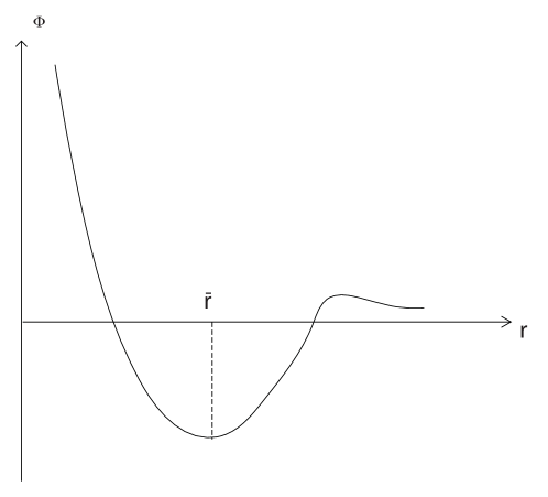
Figure 6.1.

Figure 6.1 shows that $\Phi$ has a minimum at $\bar{r}$ $(\rho<\bar{r}<r_{0})$, where the quark acting force $F$ is zero. Namely by (6.35) and (6.29), we have

(6.37) $$F=\left\{\begin{aligned} &>0&&\text{ for }0<r<\bar{r},\\ &=0&&\text{ for }r=\bar{r},\\ &<0&&\text{ for }\bar{r}<r<r_{0},\\ &>0&&\text{ for }r>r_{0}.\end{aligned}\right.$$

We infer from (6.37) the following conclusions:

1. Two close enough quarks are repelling.

2. Near $r=\bar{r}$, there are no interactions between quarks–the interactions are weak. This explains the quark asymptotic freedom phenomena.

3. In the region $\bar{r}<r<r_{0}$, the quark acting force is attracting. In particular, the attracting potential energy has the order of magnitude as

   $$\Phi\sim-\frac{c\tau}{r^{2}_{0}\rho}.$$

   It implies that

   (6.38) $$\Phi\rightarrow-\infty\ {\rm as}\ \rho\rightarrow 0,$$

   and the property (6.38) explains the quark confinement. In particular, based on (6.30) and (6.31), the ratio of binding energies of quark and nucleon is

   (6.39) $$\frac{E_{q}}{E_{n}}=\left(\frac{B}{\rho_{0}}\right)\Big{/}\left(3\left(\frac{\rho_{0}}{\rho_{1}}\right)^{3}\frac{B_{n}}{\rho_{1}}\right)\sim\left(\frac{\rho_{1}}{\rho_{0}}\right)^{4}\sim 10^{20},$$

   which is in the Planck level.

4. $F>0$ as $r>r_{0}$ means the quark attracting force is a short range force.

5. The radius $r_{0}$ represents the radius of hadrons, which is estimated as $r_{0}\leq 10^{-16}{\rm cm}$.

7. Strong Interaction Potential

7.1. QCD action for nucleons

Interaction forces act on different levels of particles/matter. Strong intersection forces are generated in three level of particles: quarks, hadrons/nucleons, and atoms. Beyond the level of atoms, the strong force almost disappears. In Section 3 we have derived the quark potential (6.29), and we devote this section to deriving hadron/nucleon and atom force potentials.

Nucleons include protons and neutrons which are the constituents of a nuclear. Classically, the force holding nucleons together to form a nuclear is the Yukawa potential

(7.1) $$\Phi_{Y}=-\frac{g}{r}e^{-k_{1}r},$$

where $k_{1}=m_{\pi}c/\hbar$ , $m_{\pi}$ is the mass of the Yukawa meson, $g$ is the meson charge with $g\cong 10e$, and $e$ is the electric charge.

The Yukawa potential (7.1) is a phenomenological theory, which provides an approximation for the short range strong interaction force between nucleons. However, formula (7.1) fails to explain the repelling phenomenon as shown in Figure 6.1 when two nucleons are close.

In the same spirit as for deriving the quark potential (6.29), we now deduce (6.34) replacing (7.1). To this end, we start with the $QCD$ action for nucleons as

(7.2) $$\mathcal{L}=-\frac{1}{4}S^{k}_{\mu\nu}S^{k\mu\nu}+\bar{n}(i\gamma^{\mu}D_{\mu}-mc^{2})n,$$

where $S^{k}_{\mu\nu}$ are as in (4.27) representing gluon fields, $n=(a_{1},a_{2},a_{3})\widetilde{n}$ with $\widetilde{n}$ being the wave function of a nucleon and $a_{1}^{2}+a_{2}^{2}+a_{3}^{2}=1$, and

(7.3) $$D_{\mu}n=(\hbar c\partial_{\mu}+ig_{s}S^{k}_{\mu}\lambda_{k})n.$$

Because the adjoint field $\phi$ of nucleons represents the $\pi$ meson-like particle field, similar to (5.31) and (5.33), from (7.2)-(7.3), we derive the field equations describing nucleons as follows

(7.4) $$\partial^{\nu}S^{k}_{\nu\mu}+\frac{g_{s}}{\hbar c}f^{kij}g^{\alpha\beta}S^{i}_{\alpha\mu}S^{j}_{\beta}-g_{s}J^{k}_{\mu}=\frac{g_{s}\zeta^{k}}{\sqrt{\hbar c}}\left(\partial_{\mu}+\frac{k^{2}_{1}}{4}x_{\mu}\right)\phi,$$

(7.5) $$i\gamma^{\mu}\left(\hbar c\partial_{\mu}+ig_{s}S^{k}_{\mu}\lambda_{k}\right)n-mc^{2}n=0,$$

where

(7.6) $$J^{k}_{\mu}=\bar{n}\gamma_{\mu}\lambda^{k}n\ \ \ \ (\lambda^{k}=\lambda_{k}),$$

(7.7) $$k_{1}=m_{\pi}c/\hbar.$$

7.2. Nucleon/hadron potential

In the same fashion as deriving (6.10), we deduce from (7.4) and (7.5) that

(7.8) $$-\nabla^{2}\phi+k^{2}_{1}\phi=g_{s}\rho^{-1}_{1}A_{n}\widetilde{\theta}_{0}\delta(r)-k^{2}_{0}\vec{x}\cdot\nabla\phi,$$

where $\rho_{1}$ is the radius of a nucleon, and

(7.9) $$A_{n}=\frac{2}{\sqrt{\hbar c}}f^{kij}\frac{\zeta^{k}\widetilde{\alpha}^{i}_{s}\xi^{j}_{\mu}}{|\zeta|^{2}}\frac{\widetilde{\theta}_{\mu}}{\widetilde{\theta}_{0}}.$$

Here $\widetilde{\theta}_{\mu}$ is defined by

(7.10) $$J^{k}_{\mu}=\alpha^{k}_{s}\widetilde{\theta}_{\mu}\delta(r).$$

The total potential equation is given by

(7.11) $$-\nabla^{2}S_{n}=g_{s}\widetilde{\theta}_{0}\delta(r)+\frac{g_{s}\zeta^{k}\widetilde{\alpha}^{k}_{s}}{4\sqrt{\hbar c}}k^{2}_{1}c\tau\phi,$$

where $\phi$ is as in (7.8), and

$$S_{n}=S^{k}_{0}\alpha^{k}_{0}$$

is the total potential of a nucleon.

Similar to (6.29), the solution of (7.11) are given by

(7.12) $$S_{n}=\widetilde{\theta}_{0}g_{s}\left[\frac{1}{r}-\frac{B_{n}k^{2}_{1}}{\rho_{1}}e^{-k_{1}r}\varphi(r)\right].$$

Here $\varphi(r)$ is as (6.26) and $B_{n}$ is a constant given by

$$B_{n}=\frac{A_{n}g_{s}\zeta^{k}\alpha^{k}_{s}}{4\sqrt{\hbar c}}c\tau,$$

$A_{n}$ is as in (7.9), $\tau$ is the lifetime of the Yukawa particle, and $k_{1}$ is as (7.7).

By (6.9) and (7.10) we have

(7.13) $$\frac{NV_{q}}{V_{n}}=\frac{|J_{0}|}{|Q_{0}|}=\frac{|\widetilde{\theta}_{0}|}{|\theta_{0}|},$$

where $V_{n}$ and $V_{q}$ are the volumes of nucleon and quark, $|J_{0}|=\sqrt{J^{k}_{0}J^{k}_{0}}$, $|Q_{0}|=\sqrt{Q^{k}_{0}Q^{k}_{0}}$, and $N=3$ is the number of quarks in a nucleon. By $V_{g}/V_{n}=\left(\frac{\rho_{1}}{\rho_{0}}\right)^{3}$, from (7.13) and $\theta_{0}=1$, we deduce that

$$\widetilde{\theta}_{0}=3\left(\frac{\rho_{0}}{\rho_{1}}\right)^{3}.$$

Thus (7.12) can be expressed as

(7.14) $$S_{n}=3\left(\frac{\rho_{0}}{\rho_{1}}\right)^{3}g_{s}\left[\frac{1}{r}-\frac{B_{n}k^{2}_{1}}{\rho_{1}}e^{-k_{1}r}\varphi(r)\right],$$

which has the same form as (6.34).

With the same method as above, an atom/molecule with $N$ nucleons generates the strong interaction potential as follows

(7.15) $$S_{a}=3N\left(\frac{\rho_{0}}{\rho_{1}}\right)^{3}\left(\frac{\rho_{1}}{\rho_{2}}\right)^{3}g_{s}\left[\frac{1}{r}-\frac{B_{n}k^{2}_{1}}{\rho_{2}}e^{-k_{1}r}\varphi(r)\right],$$

where $\rho_{2}$ is the radius of an atom, and $k_{1}$ is as in (7.14).

7.3. Physical conclusions

We have derived three formulas (6.29), (7.14) and (7.15) describing three different levels of strong interaction. The potential (6.29) reveals the hadron structure and explains the mechanism and mature of quark confinement and asymptotic freedom. Hereafter we shall see that formula (7.14) agrees with the observed data for nucleons/hadrons, and (7.15) can explain why the strong forces disappear in the macro-scale (short-range nature of the strong interaction).

We know that

$$\rho_{1}\leq 10^{-16}{\rm cm},\qquad k_{1}=10^{13}{\rm cm}^{-1},\qquad r_{1}=\frac{1}{k_{1}}=1f_{m}.$$

For the polynomial $\varphi$ in (6.26)-(6.27), we take the first-order approximation

$$\varphi=\frac{r}{2}.$$

Then (7.14) reads as

(7.16) $$S_{n}=3g_{s}\left(\frac{\rho_{0}}{\rho_{1}}\right)^{3}\left[\frac{1}{r}-\frac{10^{16}}{2}\frac{B_{n}}{r^{2}_{1}}e^{-\frac{r}{r_{1}}}r\right].$$

The force acting on one nucleon by another is

(7.17) $$F= -3g_{s}\frac{dS_{n}}{dr}$$

$$= 9g^{2}_{s}\left(\frac{\rho_{0}}{\rho_{1}}\right)^{3}\left[\frac{1}{r^{2}}-\frac{10^{16}}{2}\cdot\frac{B_{n}}{r^{2}_{1}}e^{-\frac{r}{r_{1}}}\left(\frac{r}{r_{1}}-1\right)\right]$$

$$= 9g^{2}_{s}\left(\frac{\rho_{0}}{\rho_{1}}\right)^{3}\frac{1}{r^{2}}-\frac{G_{n}}{r^{2}_{1}}\left(\frac{1}{r_{1}}-1\right)e^{-\frac{r}{r_{1}}},$$

where

$$G_{n}=\frac{9}{2}\times 10^{16}\times\left(\frac{\rho_{0}}{\rho_{1}}\right)^{3}B_{n}g^{2}_{s}.$$

With (7.1), the Yukawa force is given by

(7.18) $$F_{Y}= g^{2}\frac{d}{dr}\left(\frac{1}{r}e^{-\frac{r}{r_{1}}}\right)=-g^{2}\left(\frac{1}{r^{2}}+\frac{1}{r_{1}r}\right)e^{-\frac{r}{r_{1}}}.$$

Comparing (7.17) with (7.18), we may take

(7.19) $$g_{s}=g^{2}.$$

Namely,

$$\frac{9}{2}\times 10^{16}\times\left(\frac{\rho_{0}}{\rho_{1}}\right)^{3}B_{n}\sim 2.$$

We derive from (7.16)-(7.19) the following conclusions, consistent with experimental results:

1. The diagram of the nucleon/hadron potential (7.16) is as shown in Figure 6.1.

2. By (7.17), nucleons have a repelling radius

   $$a\cong 1f_{m},$$

   and the repelling force $F$ tends to infinite as $r\rightarrow 0$:

   $$F\rightarrow+\infty\qquad\text{\rm as }\ r\rightarrow 0.$$

3. There exists an attracting region:

   $$1f_{m}<r<zf_{m},$$

   where $z$ satisfies that

   $$z^{2}e^{-z}(z-1)=2\times 10^{-16}B^{-1}_{n}.$$

   Hence $z=30\sim 40$.

4. It is known that the radius of an atom is about

   $$\rho_{2}\cong 10^{-8}{\rm cm}.$$

   and

   $$\left(\frac{\rho_{1}}{\rho_{2}}\right)^{3}\leq 10^{-24}.$$

   In addition, the gravity and the Yukawa force are

   (7.20) $$\frac{Gm_{p}^{2}}{\hbar c}\sim 10^{-38},\qquad\frac{g^{2}}{\hbar c}\sim 10.$$

   Hence by (7.19) and (7.20), beyond the level of an atom or a molecule, the ratio between the strong repelling force and the gravitational force is

   (7.21) $$\frac{F_{s}}{F_{g}}=\left(3N^{2}\left(\frac{\rho_{0}}{\rho_{2}}\right)^{3}g_{s}^{2}\right)\Big{/}\left(N^{2}Gm_{p}^{2}\right)=3\times 10^{39}\left(\frac{\rho_{0}}{\rho_{2}}\right)^{3}.$$

   Physically, the effective quark radius is taken as $\rho\sim 10^{-21}$cm, and the atom or molecule radius is $\rho_{2}=10^{-8}$cm or $\rho_{2}=10^{-7}$cm. Then it follows from (7.21) that

   $$\frac{F_{s}}{F_{g}}\sim 3 \text{ near the atom radius }\rho_{a},$$

   $$\frac{F_{s}}{F_{g}}\sim 3\times 10^{-3} \text{ beyond the molecule radius }\rho_{m}.$$

   Namely, near the radius of an atom, the strong repelling is stronger than the gravitational force, and beyond the molecule radius, the strong repelling force is smaller than the gravitational force. We believe this competition between the gravitational force and the strong force in the level of atoms/molecules gives rise to the mechanism of the van der Waals force.

8. Duality Theory of Weak Interactions

8.1. Non-coexistence of charged and neutral particles

In Section 10, we will discuss the mass generation mechanism for the field equations (5.22) and (5.23).We focus here on charged Higgs particles and the non-coexistence of weak interaction intermediate vector bosons using these field equations.

Equation (5.22) need to be supplemented with coupling gauge equations to complement the adjoint fields $\phi_{a}$ created, which are taken as

(8.1) $$\partial^{\mu}W^{a}_{\mu}=\beta^{a}\qquad\text{ for }a=1,2,3,$$

where $\beta^{a}$ are parameters which may vary for different physical situations.

For simplicity we take the Pauli matrices $\sigma_{a}$ $(1\leq a\leq 3)$ as the generators of $SU(2)$. Then make the transformation

(8.2) $$\left(\begin{matrix}\widetilde{\sigma}_{1}\\ \widetilde{\sigma}_{2}\\ \widetilde{\sigma}_{3}\end{matrix}\right)=\left(\begin{matrix}\frac{1}{\sqrt{2}}&\frac{i}{\sqrt{2}}&0\\ \frac{1}{\sqrt{2}}&-\frac{i}{\sqrt{2}}&0\\ 0&0&1\end{matrix}\right)\left(\begin{matrix}\sigma_{1}\\ \sigma_{2}\\ \sigma_{3}\end{matrix}\right).$$

Under this transformation, $(W^{1}_{\mu},W^{2}_{\mu},W^{3}_{\mu})$ and $(\phi_{1},\phi_{2},\phi_{3})$ are transformed to

$$(W^{\pm}_{\mu},Z_{\mu})=(W^{1}_{\mu}\pm iW^{2}_{\mu},W^{3}_{\mu}),$$

$$(\phi^{\pm},\phi^{0})=(\phi_{1}\pm i\phi_{2},\phi_{3}).$$

Then by PRI, equations (5.22) become

(8.3) $$\partial^{\nu}W^{\pm}_{\nu\mu}\pm\frac{ig_{w}}{\hbar c}g^{\nu\nu}(W^{\pm}_{\nu\mu}Z_{\nu}-Z_{\nu\mu}W^{\pm}_{\nu})-g_{w}J^{\pm}_{\mu}$$

$$\qquad=\left[\partial_{\mu}-k^{2}_{W}W^{\pm}_{\mu}-k^{2}_{Z}Z_{\mu}+\frac{k_{0}^{2}}{4}x_{\mu}\right]\phi^{\pm},$$

(8.4) $$\partial^{\nu}Z_{\nu\mu}-\frac{ig_{w}}{\hbar c}g^{\nu\nu}(W^{+}_{\nu\mu}W^{-}_{\nu}-W^{-}_{\nu\mu}W^{+}_{\nu})-g_{w}J^{0}_{\mu}$$

$$\qquad=\left[\partial_{\mu}-k^{2}_{W}W^{\pm}_{\mu}-k^{2}_{Z}Z_{\mu}+\frac{k_{0}^{2}}{4}x_{\mu}\right]\phi^{0},$$

where

(8.5) $$J^{\pm}_{\mu}=\frac{1}{\sqrt{2}}(J^{1}_{\mu}\pm iJ^{2}_{\mu}),\qquad J^{NC}_{\mu}=J^{3}_{\mu},$$

$$W^{\pm}_{\nu\mu}=\partial_{\nu}W^{\pm}_{\mu}-\partial_{\mu}W^{\pm}_{\nu}\pm\frac{ig_{w}}{\hbar c}(Z_{\mu}W^{\pm}_{\nu}-Z_{\nu}W^{\pm}_{\mu}),$$

$$Z_{\nu\mu}=\partial_{\nu}Z_{\mu}-\partial_{\mu}Z_{\nu}+\frac{ig_{w}}{\hbar c}(W^{+}_{\mu}W^{-}_{\nu}-W^{-}_{\mu}W^{+}_{\nu}).$$

Here

(8.6) $$k_{W}^{2}=\frac{g_{w}\alpha_{1}^{w}}{\sqrt{2}\hbar c},\quad k_{Z}^{2}=\frac{g_{w}\alpha_{3}^{w}}{\hbar c},\quad\left(\begin{matrix}k_{W}^{2}\\ k_{W}^{2}\\ k_{Z}^{2}\end{matrix}\right)=\frac{g_{w}}{\sqrt{\hbar c}}\left(\begin{matrix}\frac{1}{\sqrt{2}}&\frac{i}{\sqrt{2}}&0\\ \frac{1}{\sqrt{2}}&-\frac{i}{\sqrt{2}}&0\\ 0&0&1\end{matrix}\right)\left(\begin{matrix}\alpha_{1}^{w}\\ \alpha_{2}^{w}\\ \alpha_{3}^{w}\end{matrix}\right),$$

where $\{\alpha^{w}_{b}\}=(\alpha^{w}_{1},\alpha^{w}_{2},\alpha_{3}^{w})$ is as in (5.22), and the second component $\alpha^{w}_{2}=0$ when we use the Pauli representation.

It is easy to see that (8.3) for $W^{+}_{\mu}$ and $W^{-}_{\mu}$ are complex conjugate to each other. Here are two important solutions, leading to two different weak interactions:

First, if

(8.7) $$W^{\pm}_{\mu}=0,\qquad\phi^{0}=1,\qquad\beta^{a}=0,$$

then $Z_{\mu}$ satisfies the equation

(8.8) $$\Box Z_{\mu}+k^{2}_{Z}Z_{\mu}-gJ^{0}_{\mu}-\frac{k_{0}^{2}}{4}x_{\mu}=0$$

where $\Box$ is the wave operator given by

$$\Box=\frac{1}{c^{2}}\frac{\partial^{2}}{\partial t^{2}}-\nabla^{2}.$$

This is the case where the weak interaction involves the neutral Higgs boson $\phi^{0}$ and the neutral intermediate vector boson $Z$ with mass parameter $k_{Z}^{2}$.

Second, if

(8.9) $$Z_{\mu}=0,\qquad\phi^{\pm}=1,\qquad\beta^{a}=0,$$

then $W^{\pm}_{\mu}$ satisfy

(8.10) $$\Box W^{\pm}_{\mu}+k^{2}_{W}W^{\pm}_{\mu}-gJ^{\pm}_{\mu}-\frac{k_{0}^{2}}{4}x_{\mu}=o(W^{\pm})$$

This is the case where the weak interaction occurs through the two charged intermediate vector bosons $W^{\pm}$, with mass parameter $k_{W}^{2}$, and the two charged Higgs bosons $\phi^{\pm}$.

These two solution cases suggest that the charged gauge bosons $W^{\pm}$ cannot appear simultaneously with the neutral boson $Z$ in one physical situation.

Now we consider the adjoint fields $\phi^{\pm}$ and $\phi^{0}$. If

(8.11) $$Z_{\mu}=0,\ \ \ \ \beta^{1}<0,\ \ \ \ \beta^{2}=0,$$

taking divergence on both sides of (8.3) we get

(8.12) $$\Box\phi^{\pm}+(k_{0}^{2}+k_{W}^{2}|\beta^{1}|)\phi^{\pm}+g_{w}\partial^{\mu}J^{\pm}_{\mu}=o(W^{\pm},\phi^{\pm}).$$

Also, if

(8.13) $$W^{\pm}_{\mu}=0,\qquad\beta^{3}<0,$$

then we obtain from (8.4) that

(8.14) $$\Box\phi^{0}+(k^{2}_{0}+k_{Z}^{2}|\beta^{3}|)\phi^{0}+g\partial^{\mu}J^{0}_{\mu}=o(Z,\phi^{0}).$$

Hence these two cases suggest also that there exist charged and neutral Higgs particles $\phi^{\pm}$ and $\phi^{0}$, and the charged Higgs $\phi^{\pm}$ cannot coexist with the neutral Higgs $\phi^{0}$.

In summary, from the above discussion we deduce the following physical conclusions:

• Existence of charged and neutral Higgs particles $\phi^{\pm}$ and $\phi^{0}$, satisfying equations (8.12) and (8.14) respectively.

• Non-coexistence of charged and neutral weak interaction particles. Namely, $W^{\pm}$ and $\phi^{\pm}$ cannot coexist with $Z$ or $\phi^{0}$.

• Finally, the two parameters $k_{0}^{2}+k_{W}^{2}|\beta^{1}|$ and $k_{o}^{2}+k_{Z}^{2}|\beta^{3}|$ define the masses $m^{c}_{H}$ and $m_{H}^{0}$ of the Higgs bosons $\phi^{\pm}$ and $\phi^{0}$. We have

  $$\frac{(m^{c}_{H})^{2}}{(m^{0}_{H})^{2}}=\frac{k_{0}^{2}+k^{2}_{W}}{k_{0}^{2}+k^{2}_{Z}}\frac{|\beta^{1}|}{|\beta^{3}|}=\frac{m_{0}^{2}+m^{2}_{W}|\beta^{1}|}{m_{0}^{2}+m^{2}_{Z}|\beta^{3}|},$$

  where $m_{0}$ is the mass associated with the mass potential $k_{0}$. We conjecture that the masses $m^{c}_{H}$ and $m^{0}_{H}$ of $\phi^{\pm}$ and $\phi^{0}$ also satisfy the scale relation (8.19), i.e.

  (8.15) $$\frac{m^{c}_{H}}{m^{0}_{H}}=\frac{m_{W}}{m_{Z}}=\frac{|j^{\pm}|}{|j^{NC}_{\mu}|}=\cos\theta_{W}.$$

  where $\theta_{W}$ is the Weinberg angle.

We remark that Conclusions 1) and 2) above cannot be derived from the classical weak interaction theories.

8.2. Scaling relation

We know from (10.36) that

(8.16) $$\frac{m_{W}}{m_{Z}}=\cos\theta_{W}.$$

According to the IVB theory for weak interaction, the charged and the neutral currents are

(8.17) $$j^{\pm}_{\mu}=\frac{g_{w}}{\sqrt{2}}J^{\pm}_{\mu},\qquad j^{NC}_{\mu}=\frac{g_{w}}{\cos\theta_{W}}J^{NC}_{\mu}.$$

After proper scaling for $J^{\pm}_{\mu}$, i.e. taking $\frac{1}{\sqrt{2}}J^{\pm}_{\mu}$ as $J^{\pm}_{\mu}$, (8.17) can be rewritten as

$$j^{\pm}_{\mu}=g_{w}J^{\pm}_{\mu},\ \ \ \ j^{NC}_{\mu}=\frac{g_{w}}{\cos\theta_{W}}J^{NC}_{\mu},$$

Hence we can consider $g_{w}$ and $g_{w}/\cos\theta_{W}$ as the intensities of the currents $j^{\pm}_{\mu}$ and $j^{NC}_{\mu}$ respectively, denoted by

(8.18) $$|j^{\pm}_{\mu}|=g_{w},\qquad|j^{NC}_{\mu}|=\frac{g_{w}}{\cos\theta_{W}}.$$

Therefore, from (8.16) and (8.18) we get the scale relation between masses and intensities of currents as

(8.19) $$\frac{|j^{\pm}_{\mu}|}{|j^{NC}_{\mu}|}=\frac{m_{W^{\pm}}}{m_{Z}}=\cos\theta_{W}.$$

By PRI, the weak interaction can be decoupled with other interactions. If we use the Pauli matrices $\sigma_{1},\sigma_{2}$ and $\sigma_{3}$ as the generators for $SU(2)$, then $G_{ab}$ is Euclidean. However, the corresponding action density $\mathcal{L}_{W}$ does not lead to the scaling relation (8.19). To solve this problem, we take another $SU(2)$ representation with the following generators:

(8.20) $$\tau_{1}=\sigma_{1},\qquad\tau_{2}=\sigma_{2},\qquad\tau_{3}=\sqrt{\cos\theta_{W}}\sigma_{3}.$$

In this case, the metric $G_{ab}$ defined by (3.19) is

$$G_{ab}=\left(\begin{matrix}1&0&0\\ 0&1&0\\ 0&0&\cos\theta_{W}\end{matrix}\right).$$

By (3.20) the action density corresponding to the representation (8.20) is given by

(8.21) $$\mathcal{L}_{W}= -\frac{1}{4}[W^{1}_{\mu\nu}W^{1\mu\nu}+W^{2}_{\mu\nu}W^{2\mu\nu}+\cos\theta_{W}W^{3}_{\mu\nu}W^{3\mu\nu}]$$

$$\qquad+\bar{L}[i\gamma^{\mu}(\partial_{\mu}-ig_{w}W^{a}_{\mu\nu}\tau_{a})-m^{L}]L,$$

where

(8.22) $$W^{a}_{\mu\nu}=\partial_{\mu}W^{a}_{\nu}-\partial_{\nu}W^{a}_{\mu}+\frac{g_{w}}{\hbar c}\lambda^{a}_{bc}W^{b}_{\mu}W^{c}_{\nu},$$

and $\lambda^{a}_{bc}$ are the structural constants with respect to (8.20), which are antisymmetric for all indices $a,b,c$.

Thus, under the ${\rm div}_{A}$-free constraint associated with

$$D_{\mu 1}=\partial_{\mu}-\left(\frac{m_{W}c}{\hbar}\right)^{2}W^{1}_{\mu}+\frac{k_{0}^{2}}{4}x_{\mu},$$

$$D_{\mu 2}=\partial_{\mu}-\left(\frac{m_{W}c}{\hbar}\right)^{2}W^{2}_{\mu}+\frac{k_{0}^{2}}{4}x_{\mu},$$

$$D_{\mu 3}=\cos\theta_{W}\partial_{\mu}-\frac{1}{\cos\theta_{W}}\left(\frac{m_{W}c}{\hbar}\right)^{2}W^{3}_{\mu}+\cos\theta_{W}\frac{k_{0}^{2}}{4}x_{\mu},$$

the Euler-Lagrangian equations of (8.21)-(8.22) are as follows

(8.23) $$\partial^{\nu}W^{1}_{\nu\mu}+k^{2}\phi W^{1}_{\mu}-\frac{g_{w}g^{\nu\nu}}{\hbar c}(W^{2}_{\nu\mu}W^{3}_{\nu}-W^{3}_{\nu\mu}W^{2}_{\nu})$$

$$\qquad\qquad-g_{w}J^{1}_{\mu}=\left[\partial_{\mu}+\frac{k_{0}^{2}}{4}x_{\mu}\right]\phi,$$

$$\partial^{\nu}W^{2}_{\nu\mu}+k^{2}\phi W^{2}_{\mu}-\frac{g_{w}g^{\nu\nu}}{\hbar c}(W^{3}_{\nu\mu}W^{1}_{\nu}-W^{1}_{\nu\mu}W^{3}_{\nu})$$

$$\qquad\qquad-g_{w}J^{2}_{\mu}=\left[\partial_{\mu}+\frac{k_{0}^{2}}{4}x_{\mu}\right]\phi,$$

$$\partial^{\nu}W^{3}_{\nu\mu}+\frac{k^{2}}{\cos^{2}\theta_{W}}\phi W^{3}_{\mu}-\frac{g_{w}}{\hbar c\cos\theta_{W}}g^{\nu\nu}(W^{1}_{\nu\mu}W^{2}_{\nu}-W^{2}_{\nu\mu}W^{1}_{\nu})$$

$$\qquad\qquad-\frac{g_{w}}{\cos\theta_{W}}J^{3}_{\mu}=\left[\partial_{\mu}+\frac{k_{0}^{2}}{4}x_{\mu}\right]\phi,$$

where $k=m_{W}c/\hbar$. Under the unitary rotation transformation

(8.24) $$\left(\begin{matrix}W^{+}_{\mu}\\ W^{-}_{\mu}\\ Z_{\mu}\end{matrix}\right)=\left(\begin{matrix}\frac{1}{\sqrt{2}}&\frac{i}{\sqrt{2}}&0\\ \frac{1}{\sqrt{2}}&-\frac{i}{\sqrt{2}}&0\\ 0&0&1\end{matrix}\right)\left(\begin{matrix}W^{1}_{\mu}\\ W^{2}_{\mu}\\ W^{3}_{\mu}\end{matrix}\right).$$

By PRI, the equations (8.23) becomes

(8.25) $$\partial^{\nu}W^{\pm}_{\nu\mu}+k^{2}\phi W^{\pm}_{\mu}\pm\frac{ig_{w}}{\hbar c}g^{\nu\nu}(W^{\pm}_{\nu\mu}Z_{\nu}-Z_{\nu\mu}W^{\pm}_{\nu})$$

$$\qquad\qquad-g_{w}J^{\pm}_{\mu}=\eta^{\pm}\left[\partial_{\mu}+\frac{k_{0}^{2}}{4}x_{\mu}\right]\phi,$$

$$\partial^{\nu}Z_{\nu\mu}+\frac{k^{2}}{\cos^{2}\theta_{W}}\phi Z_{\mu}-\frac{ig_{w}}{\hbar c\cos\theta_{W}}g^{\nu\nu}(W^{+}_{\nu\mu}W^{-}_{\nu}-W^{-}_{\nu\mu}W^{+}_{\nu})$$

$$\qquad\qquad-\frac{g_{w}}{\cos\theta_{W}}J^{NC}_{\mu}=\left[\partial_{\mu}+\frac{k_{0}^{2}}{4}x_{\mu}\right]\phi,$$

where $J^{\pm}_{\mu}$, $J^{NC}_{\mu}=J^{3}_{\mu}$ and $W^{\pm}_{\nu\mu}$, $Z_{\nu\mu}$ are defined (8.5). It is clear that for (8.25), scaling relation (8.19) holds true.

Note here that the 2nd-order $SU(2)$ tensor diag $(k^{2},k^{2},k^{2}/\cos^{2}\theta_{W})$ are invariant for the transformation (8.24). Namely

$$\left(\begin{matrix}k^{2}&0&0\\ 0&k^{2}&0\\ 0&0&\frac{k^{2}}{\cos^{2}\theta_{W}}\end{matrix}\right)=\left(\begin{matrix}\frac{1}{\sqrt{2}}&\frac{i}{\sqrt{2}}&0\\ \frac{1}{\sqrt{2}}&-\frac{i}{\sqrt{2}}&0\\ 0&0&1\end{matrix}\right)\left(\begin{matrix}k^{2}&0&0\\ 0&k^{2}&0\\ 0&0&\frac{k^{2}}{\cos^{2}\theta_{W}}\end{matrix}\right)\left(\begin{matrix}\frac{1}{\sqrt{2}}&\frac{i}{\sqrt{2}}&0\\ \frac{1}{\sqrt{2}}&-\frac{i}{\sqrt{2}}&0\\ 0&0&1\end{matrix}\right)^{\dagger}.$$

Hence from (8.23) to (8.25) we have

$$\left(k^{2}\phi W^{1}_{\mu},k^{2}\phi W^{2}_{\mu},\frac{k^{2}}{\cos^{2}\theta_{W}}\phi W^{3}_{\mu}\right)\longrightarrow\left(k^{2}\phi W^{+}_{\mu},k^{2}\phi W^{-}_{\mu},\frac{k^{2}\phi}{\cos^{2}\theta_{W}}Z_{\mu}\right).$$

Remark 8.1.

In (8.19), the ratio between the mass loss and intensity loss of the charged bosons $W^{\pm}$ and charged currents $j^{\pm}$ is the same as the ratio between those of $Z$ and $j^{NC}$. The parts lost can be considered as being transformed into electromagnetic energy.

9. Weak Interaction Potentials

9.1. Weak interaction potentials

We now consider the duality between $\{W^{a}_{\mu}\}$ and a single neutral Higgs field given by (5.26). It is clear that both the weak gauge fields $W^{a}_{\mu}$ and the adjoint scalar field $\phi$ carry rich physical information, as the electromagnetic potential $A_{\mu}$ in QED. For example, the electric field $E$ and magnetic field $H$ are written as

$$E=-\left(\frac{\partial\vec{A}}{\partial x^{0}}+\nabla A_{0}\right),\ \ \ \ H=\text{\rm curl}\vec{A},$$

where $\vec{A}=(A_{1},A_{2},A_{3}),\nabla=\left(\frac{\partial}{\partial x^{1}},\frac{\partial}{\partial x^{2}},\frac{\partial}{\partial x^{3}}\right)$, the electromagnetic energy density $\varepsilon$ is

$$\varepsilon=\frac{1}{8\pi}(E^{2}+H^{2}),$$

and the photon $\gamma$ is expressed by $A_{\mu}$ satisfying

$$\Box A_{\mu}=0.$$

So far, very little information has been extrapolated from the weak gauge fields. For example, we know that $Z_{\mu}$ and $W^{\pm}_{\mu}$ satisfying (8.8) and (8.10) represent the neutral and charged bosons, and $\phi^{\pm},\phi^{0}$ satisfying (8.12) and (8.14) represent the neutral and charged Higgs particles.

In the same spirit as electromagnetism, we introduce below two physical quantities associated with the weak gauge potentials $W^{a}_{\mu}$.

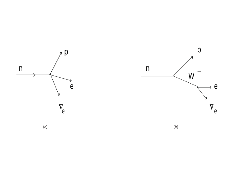
Figure 9.1.

First, the $\beta$-decay is a weak process, as illustrated by Figure 9.1 (a) and (b). Physically, the process in Figure 9.1 (a) is regarded as an exchange of a massive vector meson $W^{-}$, as shown in (b). The force range is about $r=10^{-16}$cm. Before the $\beta$-decay, the neutron $n$ is an energy pack bound by the potential energy $\phi$ in the radius $r=10^{-16}$, and when the momentum energy in the interior of a neutron is greater than the bounding energy, the neutron is split into a proton $p$ and an intermediate vector boson $W^{-}$, and the $\beta$-decay occurs. The interior momentum energy is characterized by

(9.1) $$M=\int G_{ab}\nabla W^{a}_{\mu}\nabla W^{b}_{\mu}dy,\ \ \ \ y\in\mathbb{R}^{3},$$

where $\nabla=\left(\frac{\partial}{\partial x_{1}},\frac{\partial}{\partial x_{2}},\frac{\partial}{\partial x_{3}}\right)$. Obviously, the right-hand side of (9.1) obeys PRI. Since $\varepsilon$ is the momentum energy, it is not Lorentz invariant.

Second, the weak gauge potential $W^{a}_{\mu}$ have three constituents:

$$\{W^{1}_{\mu},W^{2}_{\mu},W^{3}_{\mu}\}.$$

The time-components $W^{a}_{0}$ represent the weak-charge potentials with corresponding forces exerted by a particle with one weak charge $g_{w}$ on another with $N$ weak charges given by:

$$F_{WE}^{a}=-Ng_{w}\nabla W^{a}_{0}\qquad\text{ for }a=1,2,3.$$

The total force exerted on the particle is

(9.2) $$F_{WE}=-Ng_{w}\alpha^{w}_{a}\nabla W^{a}_{0},$$

where $\alpha^{w}_{a}$ is as in (5.22).

The spatial components $\vec{W}^{a}=(W^{a}_{1},W^{a}_{2},W^{a}_{3})$ represent the weak-rotational potentials, yielding the following weak-rotational forces:

(9.3) $$F^{a}_{WM}=g_{w}\varepsilon^{abc}\vec{J}^{b}\times\text{ curl}\vec{W}^{c},$$

$$F_{WM}=g_{w}\varepsilon^{abc}\alpha_{a}^{w}\vec{J}^{b}\times\text{ curl}\vec{W}^{c},$$

where $\{\vec{J}^{b}\}=\{J^{b}_{1},J^{b}_{2},J^{b}_{3}\}$ is the weak current density. Obviously, $F_{WE}$ and $F_{WM}$ are gauge group representation invariant, i.e. they obey PRI.

9.2. Dual field potential

We take the Pauli matrices $\sigma_{a}$ as the generators of an $SU(2)$ representation. Thus, $G_{ab}=\delta_{ab}$ and we derive from (5.27) the following equation

(9.4) $$\Box\phi+\left(\frac{m_{H}c}{\hbar}\right)^{2}\phi+\frac{\xi^{a}}{\sqrt{\hbar c}}\alpha^{w}_{b}W^{b}_{\mu}D^{\mu}\phi$$

$$\qquad=-\sqrt{\hbar c}\xi^{a}\left[\partial^{\mu}J_{\mu a}+\frac{g_{w}}{\hbar c}\lambda^{b}_{cd}g^{\alpha\beta}\partial^{\mu}(W^{c}_{\alpha\mu}W^{d}_{\beta})\right],$$

where $\xi^{a}=\zeta^{a}/|\zeta|^{2}$ ($\zeta^{a}=\zeta_{a}$).

Assume that $\phi$ and $W^{a}_{\mu}$ are small and are independent of time variable $x_{0}=ct$. Ignoring the higher order terms, equation (9.4) becomes

(9.5) $$\nabla^{2}\phi-\left(\frac{m_{H}c}{\hbar}\right)^{2}\phi=-\sqrt{\hbar c}\xi^{a}\partial^{\mu}J_{\mu a}.$$

Equation (9.5) provides a model describing the scalar potential $\phi$ of weak force, which holds energy to form a particle.

By definition, we have

$$\partial^{\mu}J_{\mu a}=\partial_{\mu}\bar{L}\gamma^{\mu}\sigma_{a}L+\bar{L}\gamma^{\mu}\sigma_{a}\partial_{\mu}L.$$

By the Dirac equation (5.23).

$$\partial_{\mu}\bar{L}\gamma^{\mu}\sigma_{a}L=-ig_{w}W^{b}_{\mu}\bar{L}\gamma^{\mu}\sigma_{b}\sigma_{a}L+im\bar{L}\sigma_{a}L,$$

$$\bar{L}\gamma^{\mu}\sigma_{a}\partial_{\mu}L=ig_{w}W^{b}_{\mu}\bar{L}\gamma^{\mu}\sigma_{a}\sigma_{b}L-im\bar{L}\sigma_{a}L.$$

Thus we obtain

$$\partial^{\mu}J_{\mu a}=ig_{w}W^{b}_{\mu}\bar{L}\gamma^{\mu}[\sigma_{a},\sigma_{b}]L=-2g_{w}\varepsilon_{abc}W^{b}_{\mu}J^{\mu}_{c}.$$

Noting that

$$\varepsilon_{abc}\xi^{a}W^{b}_{\mu}=\left|\begin{matrix}\vec{i}&\vec{j}&\vec{k}\\ \xi^{1}&\xi^{2}&\xi^{3}\\ W^{1}_{\mu}&W^{2}_{\mu}&W^{3}_{\mu}\end{matrix}\right|=\vec{\xi}\times\vec{W}_{\mu}$$

where $\vec{\xi}=(\xi^{1},\xi^{2},\xi^{3}),\vec{W}_{\mu}=(W^{1}_{\mu},W^{2}_{\mu},W^{3}_{\mu})$. Hence we obtain that

(9.6) $$\xi^{a}\partial^{\mu}J_{\mu a}=2g_{w}(\vec{\xi}\times\vec{W}_{\mu})\cdot\vec{J}^{\mu},\qquad\vec{J}^{\mu}=(J^{\mu}_{1},J^{\mu}_{2},J^{\mu}_{3}).$$

The weak charge densities $J^{a}_{0}=J^{0}_{a}$ are

(9.7) $$J_{0}^{a}=\alpha^{a}_{w}\delta(x)\qquad\text{ for }a=1,2,3,$$

where $\vec{\alpha}_{w}=(\alpha^{1}_{w},\alpha^{2}_{w},\alpha^{3}_{w})$ is as in (5.22). Therefore it follows from (9.6) that

(9.8) $$\xi^{a}\partial^{\mu}J_{\mu a}=2g_{w}\vec{\alpha}_{w}\cdot(\vec{\xi}\times\vec{W}_{\mu})\delta(x),$$

where $\vec{\omega}=\vec{W}_{0}(0),\vec{\xi}=(\zeta_{1},\zeta_{2},\zeta_{3})/|\zeta|^{2}$, and

(9.9) $$\kappa=2\vec{\alpha}_{w}\cdot(\vec{\xi}\times\vec{\omega})=2\vec{\xi}\cdot(\vec{\omega}\times\vec{\alpha}_{w})=\left|\begin{array}[]{ccc}\xi^{1}&\xi^{2}&\xi^{3}\\ \omega^{1}&\omega^{2}&\omega^{3}\\ \alpha_{w}^{1}&\alpha_{w}^{2}&\alpha_{w}^{3}\end{array}\right|.$$

Thus, by (9.8) and (9.9) the equation (9.5) is rewritten as

(9.10) $$\nabla^{2}\phi-\left(\frac{m_{H}c}{\hbar}\right)^{2}\phi=-\kappa g_{w}\delta(x).$$

Let

(9.11) $$k_{H}=\frac{m_{H}c}{\hbar},$$

where $m_{H}$ is the mass of a Higgs particle.

By (9.10) we derive the dual field potential $\phi$:

(9.12) $$\phi=\frac{\kappa g_{w}}{r}e^{-k_{H}r}.$$

Formula (9.12) leads to a few physical conclusions for weak interaction as follows:

1). The masses $m_{H}$ and $m_{\pi}$ of the Higgs and $\pi$ meson are

$$m_{H}\cong 125\ GeV/c^{2},\qquad m_{\pi}=0.135\ GeV/c^{2},$$

which implies that

$$m_{H}/m_{\pi}\cong 10^{3}.$$

By (9.12) we have

$$\frac{r_{W}}{r_{S}}=\frac{m_{\pi}}{m_{H}}=10^{-3},$$

where $r_{W}$ and $r_{S}$ are the force ranges of weak and strong interactions. Hence the weak force range is $r_{W}=10^{-16}{\rm cm},$ consistent with experimental data.

2). By (9.12), the $SU(2)$ coupling constant $g_{w}$ in (8.22) is endowed with a new physical meaning as the weak charge, reminiscent of the electric charge $e$.

3). The weak force parameter $\kappa$ given by (9.9) is an $SU(2)$ pseudo-scalar. In addition, since the quantities $\omega^{a}=W^{a}_{0}(0)$ and $\theta^{a}$ defined by (9.7) characterize the interior properties of weak interaction particles such as the electron $e$, the neutron $n$ and the proton $p$, the parameter $\kappa$ reflects the interior structure of $e,n,p$.

4). For a particle, e.g. for the neutron $n$, we conjecture that the condition for decay depends on if the interior momentum $M$ defined by (9.1) satisfies the following condition

(9.13) $$M\geq\int_{|y|<r_{0}}\frac{g_{w}^{2}}{(\hbar c)^{3/2}}\zeta^{a}\alpha^{b}_{w}W^{a}_{\mu}W^{b}_{\mu}\phi dy,\ y\in\mathbb{R}^{3},\ r_{0}=k^{-1}_{0}.$$

In this case, $n$ decays as

$$n\rightarrow p+e+\bar{\nu}_{e}.$$

Otherwise, if

(9.14) $$M<\int_{|y|<r_{0}}\frac{g_{w}^{2}}{(\hbar c)^{3/2}}\zeta^{a}\alpha^{b}_{w}W^{a}_{\mu}W^{b}_{\mu}\phi dy,$$

the neutron $n$ does not decay. Hence this explains why neutrons can spontaneously undergo a $\beta$-decay under proper conditions.

5). By (9.9), $\kappa$ can be expressed as

$$\kappa=|\vec{\theta}|\cdot|\vec{\omega}|\cos\Phi\sin\varphi,$$

where $\Phi$=the angle between $\vec{\xi}$ and $(\vec{\omega}\times\vec{\theta})$, and $\varphi=$ the angle between $\vec{\omega}$ and $\vec{\theta}$.

6). The parameter $\kappa$ may be related with weak decay coupling constants, or equivalently with the Cabibbo-Kobayashi-Maskawa angles. Hence $\kappa$ influences decay types.

9.3. Weak decay conditions

When a weak process is coupled with some external fields, energy exchange occurs. In general, gravity is much weaker than electromagnetic and strong interactions. Hence, ignoring the gravitational terms, the weak interacting field equations coupling external forces can be written as

(9.15) $$\partial^{\nu}W^{a}_{\nu\mu}-\frac{g_{w}}{\hbar c}\varepsilon^{abc}g^{\nu\nu}W^{b}_{\nu\mu}W^{c}_{\nu}-g_{w}J^{a}_{\mu}$$

$$=\frac{g_{w}}{\sqrt{\hbar c}}\zeta^{a}\left[\partial_{\mu}+\frac{e}{\hbar c}A_{\mu}+\frac{g_{w}\alpha^{b}_{w}}{\hbar c}W^{b}_{\mu}+\frac{g_{s}\alpha^{k}_{s}}{\hbar c}S^{k}_{\mu}+\frac{k_{H}^{2}}{4}x_{\mu}\right]\phi,$$

where $\{\alpha^{s}_{k}\}=(\alpha^{s}_{1},\cdots,\alpha^{s}_{8})$ is the $SU(3)$ tensor, $S^{k}_{\mu}$ $(1\leq k\leq 8)$ is the gauge potential of strong interaction, $e$ is the electric charge whose sign is undetermined, and $g_{s}$ is the strong charge.

As $W^{a}_{\mu}$ are the weak potential in the interior of a particle, $\phi$ is given by (9.12), and

(9.16) $$W^{a}_{\mu}=0\ \ \ \ {\rm at}\ \ \ \ r>r_{0}=\frac{1}{k_{H}}\cong 10^{-16}{\rm cm}.$$

Take the gauge

(9.17) $$\partial^{\mu}W^{a}_{\mu}={\rm const}.$$

and assume that $W^{a}_{\mu}$ are independent of $t$. Equations (9.15) are rewritten as

(9.18) $$-\nabla^{2}W^{a}_{\mu}-\frac{g_{w}^{2}}{(\hbar c)^{3/2}}\zeta^{a}\alpha^{b}_{w}\phi=g_{w}J^{a}_{\mu}+\frac{g_{w}}{\hbar c}\varepsilon^{abc}g^{\nu\nu}W^{b}_{\nu\mu}W^{c}_{\nu}$$

$$+\frac{g_{w}}{\sqrt{\hbar c}}\zeta^{a}\left[\frac{e}{\hbar c}A_{\mu}+\frac{g_{s}\alpha^{k}_{s}}{\hbar c}S_{\mu}^{k}+\frac{k_{H}^{2}}{4}x_{\mu}\right]\phi+\frac{g_{w}}{\sqrt{\hbar c}}\zeta^{a}\partial_{\mu}\phi.$$

Multiplying both sides of (9.18) by $W^{a}_{\mu}$ and integrating the sum in $y\in\mathbb{R}^{3}$ with $|y|<r_{0}=k^{-1}_{0}$, by (9.7), (9.16) and (9.17) we deduce that

(9.19) $$\int_{B_{r_{0}}}|\nabla W|^{2}dy-\int_{B_{r_{0}}}\frac{g_{w}^{2}}{(\hbar c)^{3/2}}\zeta^{a}\alpha^{b}_{w}W^{b}_{\mu}\cdot W^{a}_{\mu}\phi dy$$

$$=g_{w}\alpha_{w}^{a}\omega^{a}+\frac{g_{w}}{\hbar c}\int_{B_{r_{0}}}\varepsilon^{abc}g^{\nu\nu}W^{a}_{\mu}W^{b}_{\nu\mu}W^{c}_{\nu}dy$$

$$\qquad+\int_{B_{r_{0}}}\frac{g_{w}}{\sqrt{\hbar c}}\left[\frac{e}{\hbar c}A_{\mu}+\frac{g_{s}\alpha_{k}^{2}}{\hbar c}S_{\mu}+\frac{k_{H}^{2}}{4}x_{\mu}\right]W^{a}_{\mu}\zeta^{a}\phi dy,$$

where $\alpha_{w}^{a}$ and $\omega^{a}$ are as in (9.7) and (9.9), $\phi$ as (9.12), and $B_{r_{0}}=\{y\in\mathbb{R}^{3}|\ |y|<r_{0}\}$.

Approximatively, taking the spheric coordinates we have

(9.20) $$A=\int_{B_{r_{0}}}\frac{e^{-k_{0}r}}{r}A_{\mu}W^{a}_{\mu}\zeta^{a}dy=\frac{r^{2}_{0}}{2}|\Omega|\mathcal{A}_{\mu}\mathcal{W}_{\mu},$$

(9.21) $$S=\int_{B_{r_{0}}}\frac{e^{-k_{0}r}}{r}S_{\mu}W^{a}_{\mu}\zeta^{a}dy=\frac{r^{2}_{0}}{2}|\Omega|S_{\mu}\mathcal{W}_{\mu},$$

where $|\Omega|$ is the area of the unit sphere, and

$$\mathcal{A}_{\mu}=A_{\mu}(0),\qquad\mathcal{S}_{\mu}=\alpha_{s}^{k}S^{k}_{\mu}(0),\qquad\mathcal{W}_{\mu}=W^{a}_{\mu}(0)\zeta^{a}.$$

Let

(9.22) $$M=\int_{B_{r_{0}}}|\nabla W|^{2}dy, V=\int_{B_{r_{0}}}\frac{g_{w}^{2}}{(\hbar c)^{3/2}}\zeta^{a}\alpha^{b}_{w}W^{b}_{\mu}\cdot W^{a}_{\mu}\phi dy,$$

$$I=\int_{B_{r_{0}}}\varepsilon^{abc}g^{\nu\nu}W^{a}_{\mu}W^{b}_{\nu\mu}W^{c}_{\nu}dy, \Phi=\alpha_{w}^{a}\omega^{a},$$

$$H=\frac{1}{4}\int_{B_{r_{0}}}\frac{g_{w}}{\sqrt{\hbar c}}x_{\mu}W^{a}_{\mu}\zeta^{a}\phi dy.$$

Then (9.18) is rewritten as

(9.23) $$M-V=g_{w}\Phi+\frac{g_{w}}{\hbar c}I+\frac{\kappa eg_{w}^{2}}{\hbar c}A+\frac{\kappa g_{s}g^{2}}{\hbar c}S+\kappa g^{2}_{w}H.$$

Therefore, based on the criterion (9.13) and (9.14), we derive from (9.23) that for a particle under an external electromagnetic and strong fields $A_{\mu}$ and $S^{k}_{\mu}$, the condition that it can decay is

(9.24) $$\left[\Phi+I\right]+kg\left[\frac{e}{\hbar c}A+\frac{g_{s}}{\hbar c}S+H\right]\geq 0.$$

By (9.20)-(9.22), the first part in the right-hand side of (9.24) represents the weak field energy generated by the weak charge $g_{w}$, and the second part is the energy generated by external fields.

9.4. Weak interaction potential

By (9.2), the time-components $W^{a}_{0}$ of $W^{a}_{\mu}$ ($a=1,2,3$) represent the weak charge potentials generated by the weak charge $g_{w}$. We now derive an approximate formula for the total potential:

(9.25) $$W={\alpha^{a}_{w}W^{a}_{0}},\qquad\text{ where }|\alpha_{w}|^{2}=\alpha^{a}_{w}\alpha^{a}_{w}=1.$$

Assuming that $W^{a}_{\mu}$ are independent of time and taking linear approximation, from (5.27) we have

(9.26) $$-\nabla^{2}W={g_{w}\alpha^{a}_{w}}J_{0}^{a}+\frac{g_{w}}{\sqrt{\hbar c}}{\alpha_{w}^{a}\zeta^{a}}\left(\frac{k_{0}^{2}}{4}c\tau-\frac{g_{w}}{\hbar c}W\right)\phi,$$

where $\tau$ is the lifetime of the Higgs, and

(9.27) $$\phi=\theta+\phi_{0},$$

where $\phi_{0}$ is given by (9.12) and $\theta$ is a constant. Taking a translation

$$W\quad\longrightarrow W+\frac{k_{0}^{2}\hbar c^{2}\tau}{4g_{w}},$$

and by $J_{0}^{a}=\alpha^{a}_{w}\delta(x)$, equations (9.26) and (9.27) become

(9.28) $$-\nabla^{2}W+k_{1}^{2}W=g_{w}\delta(x)-\frac{g_{w}^{2}}{(\hbar c)^{3/2}}KW\phi_{0},$$

where

(9.29) $$k_{1}^{2}=\frac{g_{w}^{2}}{(\hbar c)^{3/2}}{\alpha_{w}^{a}\zeta^{a}}\theta,\qquad K={\alpha_{w}^{a}\zeta^{a}}.$$

Solutions of (9.28) and (9.29) can be expressed as

(9.30) $$W=W_{0}+W_{1}+\cdots,$$

where $W_{n}$ satisfy

(9.31) $$-\nabla^{2}W_{0}+k_{1}^{2}W_{0}=g_{w}\delta(x),$$

(9.32) $$-\nabla^{2}W_{n}+k_{1}^{2}W_{n}=-\left(\frac{g_{w}^{2}}{\hbar c}\right)^{3/2}\frac{A}{r}e^{-k_{1}r}W_{n-1} \text{ for }n=1,2,\cdots,$$

and $A=K\kappa.$ The solution of (9.31) is

(9.33) $$W_{0}=\frac{g_{w}}{r}e^{-k_{1}r}.$$

When $n=1$, (9.32) is given by

(9.34) $$\nabla^{2}W_{1}-k_{1}^{2}W_{1}=A\left(\frac{g_{w}^{2}}{\hbar c}\right)^{3/2}\frac{g_{w}}{r^{2}}e^{-(k_{0}+k_{1})r}.$$

Let $W_{1}$ be radial symmetric and in the form

(9.35) $$W_{1}=A\left(\frac{g_{w}^{2}}{\hbar c}\right)^{3/2}g_{w}e^{-(k_{0}+k_{1})r}\varphi_{1}(r).$$

Then (9.34) implies that

(9.36) $$\varphi_{1}^{\prime\prime}+2\left(\frac{1}{r}-K_{1}\right)\varphi_{1}^{\prime}-\frac{2K_{1}}{r}\varphi_{1}+(K_{1}^{2}-k_{1}^{2})\varphi_{1}=\frac{1}{r^{2}},$$

where $K_{1}=k_{0}+k_{1}$.

Let $\varphi_{1}$ be expanded as

(9.37) $$\varphi_{1}=\sum^{\infty}_{k=0}p_{k}r^{k}\ln r+\sum^{\infty}_{k=0}q_{k}r^{k}.$$

Inserting (9.37) into (9.36) and comparing coefficients, we deduce that

$$p_{0}=1,\qquad p_{1}=\frac{2}{3}(1+q_{0}), p_{2}=\frac{5}{18}K_{1}^{2}+\frac{1}{6}k_{1}^{2},\qquad\cdots,$$

$$q_{0}\text{ and }q_{1}\text{ are free }, q_{2}=-\frac{1}{36}K_{1}^{2}-\frac{5}{12}+K_{1}\beta_{1},\qquad\cdots.$$

Then we infer from (9.32) that

(9.38) $$W_{n}=A^{n}\left(\frac{g_{w}^{2}}{\hbar c}\right)^{3n/2}g_{w}e^{-K_{n}r}\varphi_{1}(r),\qquad K_{n}=k_{0}+nk_{1}\qquad\text{ for }n\geq 1,$$

and $\varphi_{n}$ satisfies

(9.39) $$\varphi_{n}^{\prime\prime}+2\left(\frac{1}{r}-K_{n}\right)\varphi_{n}^{\prime}-\frac{2K_{n}}{r}\varphi_{n}+(K_{n}^{2}-k_{1}^{2})\varphi_{n}=\frac{\varphi_{n-1}}{r}.$$

The solution of this equation is in the form

(9.40) $$\varphi_{n}=\sum^{\infty}_{k=n-1}p^{n}_{k}r^{k}\ln r+\sum^{\infty}_{k=n-1}q^{n}_{k}r^{k},$$

where $p^{n}_{k}$ and $q^{n}_{k}$ depend on the free parameters $q_{0}$ and $q_{1}$.

Hence by (9.30) and (9.38), the solution $W$ of (9.28) can be expressed as

(9.41) $$W=g_{w}e^{-k_{1}r}\left[\frac{1}{r}-\sum^{\infty}_{n=1}A^{n}\left(\frac{g_{w}^{2}}{\hbar c}\right)^{3n/2}e^{-(k_{0}+(n-1)k_{1})r}\psi_{n}\right],$$

where $\psi_{n}=-\varphi_{n}$ and $\varphi_{n}$ is given by (9.40).

The function $\Psi=e^{-k_{0}r}\psi$ with

$$\psi=\sum^{\infty}_{n=1}A^{n}\left(\frac{g_{w}^{2}}{\hbar c}\right)^{3n/2}g_{w}e^{-nk_{1}r}\psi_{n}$$

is the solution of

(9.42) $$\frac{1}{r^{2}}\frac{d}{dr}\left(r^{2}\frac{d}{dr}\right)\Psi-k_{1}^{2}\Psi=-\left(\frac{g_{w}^{2}}{\hbar c}\right)^{3/2}\frac{A}{r}e^{-k_{1}r}\Psi-\left(\frac{g_{w}^{2}}{\hbar c}\right)^{3/2}\frac{Ag_{w}}{r^{2}}e^{-(k_{0}+k_{1})r}.$$

Now we supply $\psi$ with the following initial conditions:

(9.43) $$\psi(r_{1})=a_{0},\qquad\psi^{\prime}(r_{1})=a_{1}\qquad\text{ at }r_{1}>0.$$

In summary, we have derived the weak potential and weak force formula given by

(9.44) $$W=g_{w}e^{-k_{1}r}\left[\frac{1}{r}-e^{-k_{0}r}\psi(r)\right],$$

(9.45) $$F=g_{w}^{2}e^{-k_{1}r}\left[\frac{k_{1}}{r}+\frac{1}{r^{2}}-(K_{1}\psi-\psi^{\prime})e^{-k_{0}r}\right],$$

where $K_{1}=k_{0}+k_{1}$, $k_{0}=m_{H}c/\hbar$, $k_{1}=m_{W}c/\hbar$, $m_{H}$ and $m_{W}$ are the masses of the Higgs and $W^{\pm}$ or $Z$ bosons, and by (9.43), $\psi(r)$ can be approximately written as

(9.46) $$\psi(r)=a_{0}+a_{1}r\qquad\text{ near }r=r_{1}=\frac{1}{k_{0}}.$$

Thus the weak force becomes

(9.47) $$F=g_{w}^{2}e^{-k_{1}r}\left[\frac{k_{1}}{r}+\frac{1}{r^{2}}-(a_{0}-a_{1}+a_{1}r)e^{-k_{0}r}\right].$$

Based on known physical facts, we have

(9.48) $$a_{0}>0,\qquad a_{1}\leq 0,\qquad a_{0}-a_{1}\gg k_{1}^{2}.$$

Hence we have derived the following physical conclusions:

1. A particle with weak charge $g_{w}$ will generate a weak force $F$ exerted on another with weak charge $g_{w}$, and the force $F$ is given by (9.45) or (9.47).

2. By (9.41 and (9.45), there is a radius $r_{0}>0$ such that $F$ is repelling for $r<r_{0}$, and

   $$F\to\infty\quad\text{ as }r\to 0.$$

3. By (9.47) and (9.48), $F$ has an attractive region: $r_{0}<r<r_{1}$.

4. The weak interaction force $F$ is of short-range:

   $$F\sim 0\quad\text{ for }r>\frac{1}{k_{1}}\sim 10^{-16}cm.$$

10. Consistency with GWS Electroweak Theory

The main objective of this section is to study the consistency of the new electroweak theory based on PID and PRI with the classical GWS electroweak theory.

10.1. GWS action

For comparison, we first introduce the classical Glashow-Weinberg-Salam electroweak theory, which is a $U(1)\otimes SU(2)$ gauge theory. We adopt here the classical notations. The action is given by

(10.1) $$L_{GWS}=\int[\mathcal{L}_{G}+\mathcal{L}_{F}+\mathcal{L}_{H}]dx.$$

Here $\mathcal{L}_{G}$ is the gauge part, $\mathcal{L}_{F}$ is the fermionic part, and $\mathcal{L}_{H}$ is the Higgs sector:

(10.2) $$\mathcal{L}_{G}=-\frac{1}{4}W^{a}_{\mu\nu}W^{\mu\nu a}-\frac{1}{4}B_{\mu\nu}B^{\mu\nu},$$

$$\mathcal{L}_{F}=i\bar{L}\gamma^{\mu}D_{\mu}L+i\bar{e}^{R}\gamma^{\mu}D_{\mu}e^{R},$$

$$\mathcal{L}_{H}=D_{\mu}\phi^{\dagger}D^{\mu}\phi+\lambda(\phi^{\dagger}\phi-a^{2})^{2}+G_{e}(\bar{L}\phi e^{R}+\bar{e}^{R}\phi^{\dagger}L),$$

where $G_{e}$ and $a>0$ are constants, $L=(\nu_{e},e^{L})$, $e^{R}$ is the wave function of right-hand electron, $\phi$ is the Higgs scalar field, and

$$W^{a}_{\mu\nu}=\partial_{\mu}W^{a}_{\nu}-\partial_{\nu}W^{a}_{\mu}+g_{1}\varepsilon^{abc}W^{b}_{\mu}W^{c}_{\nu},$$

$$B_{\mu\nu}=\partial_{\mu}B_{\nu}-\partial_{\nu}B_{\mu},$$

$$D_{\mu}e^{R}=(\partial_{\mu}+ig_{2}B_{\mu})e^{R},$$

$$D_{\mu}L=(\partial_{\mu}+i\frac{g_{2}}{2}B_{\mu}-i\frac{g_{1}}{2}W^{a}_{\mu}\sigma_{a})L,$$

$$D_{\mu}\phi=(\partial_{\mu}-i\frac{g_{2}}{2}B_{\mu}-i\frac{g_{1}}{2}W^{a}_{\mu}\sigma_{a})\phi,$$

Here $g_{1}$ and $g_{2}$ are coupling constants, $\varepsilon^{kij}$ ($1\leq k,i,j\leq 3$) are the structural constants of $SU(2)$, $\sigma_{k}$ ($1\leq k\leq 3$) are the Pauli matrices, $\{W^{a}_{\mu}\}$ is the Yang-Mills gauge field corresponding to the k-th generator of $SU(2)$, and $\{B_{\mu}\}$ is the gauge field with respect to $U(1)$.

We note that $B_{\mu}$ does not represent the electromagnetic potential $A_{\mu}$, and the Higgs field $\phi$ is a complex doublet given by

$$\phi=(\phi^{+},\phi^{0})^{T},$$

which has charge (1,0).

The action (10.1) is invariant under the $SU(2)$ gauge transformation

(10.3) $$L\rightarrow e^{\frac{i}{2}\theta^{a}\sigma_{a}}L,$$

$$\phi\rightarrow e^{-\frac{i}{2}\theta^{a}\sigma_{a}}\phi,$$

$$e^{R}\rightarrow e^{R},$$

$$W^{a}_{\mu}\rightarrow W^{a}_{\mu}-\frac{2}{g_{1}}\partial_{\mu}\theta^{a}+\varepsilon^{abc}\theta^{b}W^{c}_{\mu},$$

and the $U(1)$ gauge transformation

(10.4) $$L\rightarrow e^{\frac{i}{2}\beta}L,$$

$$\phi\rightarrow e^{-\frac{i}{2}\beta}\phi,$$

$$e^{R}\rightarrow e^{i\beta}e^{R},$$

$$W^{a}_{\mu}\rightarrow W^{a}_{\mu}-\frac{2}{g_{2}}\partial_{\mu}\beta,$$

$$B_{\mu}\rightarrow B_{\mu}+\frac{2}{g_{2}}\partial_{\mu}\beta.$$

We notice from (10.2) and (10.1) that $\mathcal{L}_{F}$ contains the following terms:

(10.5) $$W^{\mu}_{a}J^{a}_{\mu}, J^{a}_{\mu}=\bar{L}\gamma_{\mu}\sigma_{a}L.$$

These terms are crucial in the weak interaction theory because under a unitary transformation

(10.6) $$\left(\begin{matrix}\sigma^{+}\\ \sigma^{-}\\ \sigma^{0}\end{matrix}\right)=\left(\begin{matrix}\frac{1}{\sqrt{2}}&\frac{i}{\sqrt{2}}&0\\ \frac{1}{\sqrt{2}}&-\frac{i}{\sqrt{2}}&0\\ 0&0&1\end{matrix}\right)\left(\begin{matrix}\sigma_{1}\\ \sigma_{2}\\ \sigma_{3}\end{matrix}\right),$$

these terms become

(10.7) $$W^{\mu\pm}J^{\pm}_{\mu}, W^{\mu 3}J^{3}_{\mu}, W^{\pm}_{\mu}=\frac{1}{\sqrt{2}}(W^{1}_{\mu}\pm iW^{2}_{\mu}),$$

$$J^{\mu\pm}=\bar{L}\gamma^{\mu}\sigma_{\pm}L, J^{3}_{\mu}=\bar{L}\gamma_{\mu}\sigma_{3}L,$$

where $\sigma_{\pm}=\frac{1}{2}(\sigma_{1}\pm i\sigma_{2})$, and $J^{\mu\pm}$ are the charged currents consistent with the classical V-A theory and the intermediate vector boson (IVB) theory, which are two successful models at low energies.

Physically, $W^{\pm}_{\mu}$ particles are vector intermediate bosons having mass $m_{W}$, which should satisfy the Klein-Gordon equation

$$\partial^{\mu}\partial_{\mu}W^{\pm}_{\nu}+k^{2}W^{\pm}_{\nu}=o(W^{\pm}),$$

where $o(W^{\pm})$ stands for the higher order terms of $W^{\pm}$, and $k=m_{W}c/\hbar$. However, we find that the variational equations of the action (10.1) have the form

$$\frac{\delta L_{GWS}}{\delta W^{a}_{\mu}}=\partial^{\mu}W^{a}_{\mu\nu}+o(W)=0,$$

which implies that $W^{\pm}_{\mu}$ in (10.7) would be massless, contradicting with the fact that $W^{\pm}$ are massive.

Higgs mechanism provides a resolution. We see from (10.2) and (10.1) that $\phi_{0}=(0,a)^{T}$ is an extremum point of (10.1), i.e. for $\Phi=(W,B,L,R,\phi)$, $\Phi_{0}=(0,0,0,0,\phi_{0})$ is a solution of

$$\delta L_{GWS}=0.$$

Consider the translation

(10.8) $$\Phi=\Phi^{\prime}+\Phi_{0},\ \ \ \ \Phi^{\prime}=(W^{\prime},B^{\prime},L^{\prime},R^{\prime},\phi^{\prime}).$$

Then the variational equations of $L_{GWS}$ for $\Phi^{\prime}$ are given by (for simplicity, omitting the primes)

(10.9) $$\left(\begin{array}[]{l}\frac{\delta}{\delta W}L_{GWS}\\ \frac{\delta}{\delta B}L_{GWS}\end{array}\right)=\left(\begin{array}[]{l}\partial^{\mu}W_{\mu\nu}\\ \partial^{\mu}B_{\mu\nu}\end{array}\right)+M\left(\begin{array}[]{l}W_{\nu}\\ B_{\nu}\end{array}\right)+o(W,B)=0,$$

where $M$ is the mass matrix induced by $\Phi_{0}$. It is clear that (10.9) is no longer covariant, or equivalently $L_{GWS}$ breaks the symmetry for $\Phi^{\prime}$ for (10.3)-(10.3). But the particles described by $(W^{\prime},B^{\prime})$ receive masses due to the symmetry breaking.

10.2. Weinberg-Salam electroweak theory

We now recapitulate the WS electroweak theory. In (10.1)-(10.1), replace $\phi=(\phi^{+},\phi^{0})^{T}$ by $\phi=(0,\varphi)$, then the system is simplified and still invariant under the transformations (10.3) and (10.4), and avoids the difficulty that there exists a charged and massless bosonic field $\phi^{+}$ in the classical GWS model. In this case, the Higgs action in (10.2) becomes

(10.10) $$\mathcal{L}_{H}= \partial^{\mu}\varphi\partial_{\mu}\varphi+\varphi^{2}\left[\frac{g^{2}_{1}}{4}W^{a}_{\mu}W^{\mu a}+\frac{g^{2}_{2}}{4}B_{\mu}B^{\mu}-\frac{g_{1}g_{2}}{2}B^{\mu}W^{3}_{\mu}\right]$$

$$-\lambda(\varphi^{2}-a^{2})^{2}+G_{e}\varphi(\bar{e}^{L}e^{R}+\bar{e}^{R}e^{L}).$$

Then the Euler-Lagrange equations of the action (10.1) are given by

(10.11) $$\partial^{\nu}W^{1}_{\nu\mu}-g_{1}g^{\nu\nu}(W^{2}_{\nu\mu}W^{3}_{\nu}-W^{3}_{\nu\mu}W^{2}_{\nu})+\frac{g_{1}}{2}J^{1}_{\mu}+\frac{g^{2}_{1}}{2}\varphi^{2}W^{1}_{\mu}=0,$$

(10.12) $$\partial^{\nu}W^{2}_{\nu\mu}-g_{1}g^{\nu\nu}(W^{3}_{\nu\mu}W^{1}_{\nu}-W^{1}_{\nu\mu}W^{3}_{\nu})+\frac{g_{1}}{2}J^{2}_{\mu}+\frac{g^{2}_{1}}{2}\varphi^{2}W^{2}_{\mu}=0,$$

(10.13) $$\partial^{\nu}W^{3}_{\nu\mu}-g_{1}g^{\nu\nu}(W^{1}_{\nu\mu}W^{2}_{\nu}-W^{2}_{\nu\mu}W^{1}_{\nu})+\frac{g_{1}}{2}J^{3}_{\mu}+\frac{g_{1}}{2}\varphi^{2}(g_{1}w^{3}_{\mu}-g_{2}B_{\mu})=0,$$

(10.14) $$\partial^{\nu}B_{\nu\mu}-\frac{g_{2}}{2}J^{L}_{\mu}-g_{2}J^{R}_{\mu}+\frac{g_{2}}{2}\varphi^{2}(g_{2}B_{\mu}-g_{1}W^{3}_{\mu})=0,$$

(10.15) $$i\gamma^{\mu}(\partial_{\mu}+i\frac{g_{2}}{2}B_{\mu}-i\frac{g_{1}}{2}W^{a}_{\mu}\sigma_{a})\left(\begin{matrix}\nu\\ e^{L}\end{matrix}\right)+G_{e}e^{R}\left(\begin{matrix}0\\ \varphi\end{matrix}\right)=0,$$

(10.16) $$i\gamma^{\mu}(\partial_{\mu}+ig_{2}B_{\mu})e^{R}+G_{e}\varphi e^{L}=0,$$

(10.17) $$\partial^{\mu}\partial_{\mu}\varphi-\frac{1}{2}\varphi(g^{2}_{1}W^{a}_{\mu}W^{\mu a}+g^{2}_{2}B_{\mu}B^{\mu}-2g_{1}g_{2}W^{3}_{\mu}B^{\mu})$$

$$+4\lambda a^{2}\varphi-4\lambda\varphi^{3}-G_{e}(\bar{e}^{L}e^{R}+\bar{e}^{R}e^{L})=0.$$

Under the translation (10.8), or equivalently inserting

(10.18) $$\varphi=\phi_{0}+a$$

into (10.11)-(10.16) we obtain

(10.19) $$\partial^{\nu}\widetilde{W}^{1}_{\nu\mu}+\frac{g^{2}_{1}a^{2}}{2}W^{1}_{\mu}+\frac{g_{1}}{2}J^{1}_{\mu}=o(W,\phi_{0}),$$

(10.20) $$\partial^{\nu}\widetilde{W}^{2}_{\nu\mu}+\frac{g^{2}_{1}a^{2}}{2}W^{2}_{\mu}+\frac{g_{1}}{2}J^{2}_{\mu}=o(W,\phi_{0}),$$

(10.21) $$\partial^{\nu}\widetilde{W}^{3}_{\nu\mu}+\frac{g^{2}_{1}a^{2}}{2}W^{3}_{\mu}-\frac{g_{1}g_{2}a^{2}}{2}B_{\mu}+\frac{g_{1}}{2}J^{3}_{\mu}=o(W,B,\phi_{0}),$$

(10.22) $$\partial^{\nu}B_{\nu\mu}+\frac{g^{2}_{2}a^{2}}{2}B_{\mu}-\frac{g_{1}g_{2}a^{2}}{2}W^{3}_{\mu}-g_{2}J^{R}_{\mu}-\frac{g_{2}}{2}J^{L}_{\mu}=o(W,B,\phi_{0}),$$

(10.23) $$i\gamma^{\mu}D_{\mu}\nu_{e}=0,$$

(10.24) $$i\gamma^{\mu}D_{\mu}e^{L}+aG_{e}e^{R}+G_{e}\phi_{0}e^{R}=0,$$

(10.25) $$i\gamma^{\mu}D_{\mu}e^{R}+aG_{e}e^{L}+G_{e}\phi_{0}e^{L}=0,$$

where

(10.26) $$\widetilde{W}^{a}_{\nu\mu}=\partial_{\nu}W^{a}_{\mu}-\partial_{\mu}W^{a}_{\nu}, B_{\nu\mu}=\partial_{\nu}B_{\mu}-\partial_{\mu}B_{\nu}.$$

From (10.19)-(10.22) we can find the mass terms

(10.27) $$M\left(\begin{matrix}W^{1}_{\mu}\\ W^{2}_{\mu}\\ W^{3}_{\mu}\\ B_{\mu}\end{matrix}\right)=\left(\begin{matrix}\frac{g^{2}_{1}a^{2}}{2}&0&0&0\\ 0&\frac{g^{2}_{1}a^{2}}{2}&0&0\\ 0&0&\frac{g^{2}_{1}a^{2}}{2}&-\frac{g_{1}g_{2}a^{2}}{2}\\ 0&0&-\frac{g_{1}g_{2}a^{2}}{2}&\frac{g^{2}_{2}a^{2}}{2}\end{matrix}\right)\left(\begin{matrix}W^{1}_{\mu}\\ W^{2}_{\mu}\\ W^{3}_{\mu}\\ B_{\mu}\end{matrix}\right)$$

and the current terms

(10.28) $$J_{\mu}=\left(\frac{g_{1}}{2}J^{1}_{\mu},\quad\frac{g_{1}}{2}J^{2}_{\mu},\quad\frac{g_{1}}{2}J^{3}_{\mu},\quad-g_{2}J^{R}_{\mu}-\frac{g_{1}}{2}J^{L}_{\mu}\right)^{T}.$$

In order to generate masses, we have to diagonalize the matrix of (10.27), by a rotating transformation for $(W^{3}_{\mu},B_{\mu})$ as

(10.29) $$\left(\begin{matrix}Z_{\mu}\\ A_{\mu}\end{matrix}\right)=\left(\begin{matrix}\frac{g_{1}}{|g|}&\frac{g_{2}}{|g|}\\ -\frac{g_{2}}{|g|}&\frac{g_{1}}{|g|}\end{matrix}\right)\left(\begin{matrix}W^{3}_{\mu}\\ B_{\mu}\end{matrix}\right),$$

where $|g|=(g^{2}_{1}+g^{2}_{2})^{{1}/{2}}$. On the other hand, the charged currents $J^{\pm}_{\mu}$ are given by (10.7) which are derived by the transformation (10.6), or equivalently by the unitary rotation of $(W^{1}_{\mu},W^{2}_{\mu})$ as

(10.30) $$\left(\begin{matrix}W^{+}_{\mu}\\ W^{-}_{\mu}\end{matrix}\right)=\left(\begin{matrix}\frac{1}{\sqrt{2}}&\frac{i}{\sqrt{2}}\\ \frac{1}{\sqrt{2}}&-\frac{i}{\sqrt{2}}\end{matrix}\right)\left(\begin{matrix}W^{1}_{\mu}\\ W^{2}_{\mu}\end{matrix}\right).$$

Hence, under the following unitary transformation

(10.31) $$\left(\begin{matrix}W^{+}_{\mu}\\ W^{-}_{\mu}\\ Z_{\mu}\\ A_{\mu}\end{matrix}\right)=U\left(\begin{matrix}W^{1}_{\mu}\\ W^{2}_{\mu}\\ W^{3}_{\mu}\\ B_{\mu}\end{matrix}\right),\qquad U=\left(\begin{matrix}\frac{1}{\sqrt{2}}&\frac{i}{\sqrt{2}}&0&0\\ \frac{1}{\sqrt{2}}&-\frac{i}{\sqrt{2}}&0&0\\ 0&0&\frac{g_{1}}{|g|}&\frac{g_{2}}{|g|}\\ 0&0&-\frac{g_{2}}{|g|}&\frac{g_{1}}{|g|}\end{matrix}\right),$$

the mass matrix $M$ in (10.27) becomes

(10.32) $$UMU^{\dagger}=\frac{c^{2}}{\hbar^{2}}\left(\begin{matrix}m^{2}_{W}&0&0&0\\ 0&m^{2}_{W}&0&0\\ 0&0&m^{2}_{Z}&0\\ 0&0&0&0\end{matrix}\right),$$

and the current $J_{\mu}$ in (10.28) is as

(10.33) $$\left(\frac{g_{1}}{\sqrt{2}}J^{+}_{\mu},\quad\frac{g_{1}}{\sqrt{2}}J^{-}_{\mu},\quad|g|J^{NC}_{\mu},\quad eJ^{em}_{\mu}\right)^{T}=UJ_{\mu}.$$

Also, equations (10.19)-(10.22) become

(10.34) $$\partial^{\nu}(\partial_{\nu}W^{+}_{\mu}-\partial_{\mu}W^{+}_{\nu})+\left(\frac{cm_{W}}{\hbar}\right)^{2}W^{+}_{\mu}+\frac{g_{1}}{\sqrt{2}}J^{+}_{\mu}=o(\Phi),$$

$$\partial^{\nu}(\partial_{\nu}W^{-}_{\mu}-\partial_{\mu}W^{-}_{\nu})+\left(\frac{cm_{W}}{\hbar}\right)^{2}W^{-}_{\mu}+\frac{g_{1}}{\sqrt{2}}J^{-}_{\mu}=o(\Phi),$$

$$\partial^{\nu}(\partial_{\nu}Z_{\mu}-\partial_{\mu}Z_{\nu})+\left(\frac{cm_{Z}}{\hbar}\right)^{2}Z_{\mu}+|g|J^{NC}_{\mu}=o(\Phi),$$

$$\partial^{\nu}(\partial_{\nu}A_{\mu}-\partial_{\mu}A_{\nu})-eJ^{em}_{\mu}=o(\Phi),$$

where $\Phi=(W^{+},W^{-},Z,A,\phi_{0})$.

The above field equations (10.31)-(10.34) lead to the following physical conclusions as part of the classical electroweak theory:

1). When the Higgs field $\varphi$ possesses a nonzero vacuum state as (10.18), the gauge symmetry breaks, and the fields $W^{a}_{\mu}$ and $B_{\mu}$ are recombined to yield a changed doublet of massive vector intermediate bosons $W^{\pm}_{\mu}$, a neutral massive vector boson $Z_{\mu}$, and a massless photon field $A_{\mu}$:

(10.35) $$W^{\pm}_{\mu}=\frac{1}{\sqrt{2}}(W^{1}_{\mu}\pm W^{2}_{\mu}),$$

$$Z_{\mu}=\frac{1}{|g|}(g_{1}W^{3}_{\mu}+g_{2}B_{\mu})=\cos\theta_{W}W^{3}_{\mu}+\sin\theta_{W}B_{\mu},$$

$$A_{\mu}=\frac{1}{|g|}(-g_{2}W^{3}_{\mu}+g_{1}B_{\mu})=-\sin\theta_{W}W^{3}_{\mu}+\cos\theta_{W}B_{\mu},$$

where $\theta_{W}$ is the Weinberg angle defined as

$$\cos\theta_{W}=\frac{g_{1}}{|g|}=\frac{g_{1}}{\sqrt{g^{2}_{1}+g^{2}_{2}}}, \sin\theta_{W}=\frac{g_{2}}{|g|}=\frac{g_{2}}{\sqrt{g^{2}_{1}+g^{2}_{2}}}.$$

2). The masses of $W^{\pm}_{\mu}$ and $Z$ are as in (10.32) given by

(10.36) $$m_{W^{+}}=m_{W^{-}}=\frac{a\hbar}{\sqrt{2}c}g_{1},\ \ \ \ m_{Z}=\frac{a\hbar}{\sqrt{2}c}|g|$$

3). The electric charge in (10.34) is

(10.37) $$e=g_{1}\sin\theta_{W}.$$

4). Both charged currents $J^{\pm}_{\mu}$ and the neutral current $J^{NC}_{\mu}$ appearing in (10.34) are derived from (10.28) and (10.33), given by

(10.38) $$J^{\pm}_{\mu}=\frac{1}{2}(J^{1}_{\mu}\pm iJ^{2}_{\mu}), J^{NC}_{\mu}=\frac{1}{2}[\cos\theta^{2}_{W}J^{3}_{\mu}-\sin^{2}\theta_{W}J^{L}_{\mu}-2\sin^{2}\theta_{W}J^{R}_{\mu}],$$

where $J^{a}_{\mu}$ is as in (10.5), and

$$J^{3}_{\mu}=\bar{\nu}_{e}\gamma_{\mu}\nu_{e}-\bar{e}^{L}\gamma_{\mu}e^{L}, J^{R}_{\mu}=\bar{e}^{R}\gamma_{\mu}e^{R},$$

$$J^{L}_{\mu}=\bar{\nu}_{e}\gamma_{\mu}\nu_{e}+\bar{e}^{L}\gamma_{\mu}e^{L}, J^{em}_{\mu}=\frac{1}{2}J^{3}_{\mu}+\frac{1}{2}J^{L}_{\mu}+J^{R}_{\mu}=\bar{\nu}_{e}\gamma_{\mu}\nu_{e}+\bar{e}^{R}\gamma_{\mu}e^{R}.$$

Here $J^{em}_{\mu}$ is the electric current.

5). By (10.24) and (10.25) the mass of an electron is given by

(10.39) $$m_{e}=aG_{e}.$$

6). Finally, (10.17) is the Higgs field equation, from which we derive the mass of the Higgs particle as

(10.40) $$m_{H}=2a\sqrt{\lambda}.$$

Two remarks are now in order.

Remark 10.1.

From (10.39) and (10.40) we see that the electron mass $m_{e}$ and the Higgs particle mass $m_{H}$ can not be determined by the electroweak theory, and their values are also helpless for determining the masses of $W^{\pm}_{\mu}$ and $Z_{\mu}$. By the $V-A$ theory, we have

$$\frac{G_{F}}{\sqrt{2}}=\frac{g^{2}_{1}}{8m^{2}_{W}}=\frac{1}{4a^{2}},$$

where $G_{F}$ is the Fermi constant. Therefore,

(10.41) $$a^{2}=\frac{1}{2\sqrt{2}G_{F}}.$$

Experimentally the value of $\theta_{W}$ is determined by

$$\sin^{2}\theta_{W}=0.2325\pm 0.008.$$

Then, from (10.36), (10.37) and (10.41) it follows that

$$m_{W}=80.22\pm 0.26\ GeV/c^{2},$$

$$m_{Z}=91.173\pm 0.020\ GeV/c^{2}.$$

Remark 10.2.

It is worth mentioning that the transformation (10.31) corresponds to a mixed transformation of $U(1)$ generator $\sigma_{0}=1$ and $SU(2)$ generators $\sigma_{a}$:

$$\left(\begin{matrix}\tau_{1}\\ \tau_{2}\\ \tau_{3}\\ \tau_{0}\end{matrix}\right)=U\left(\begin{matrix}\sigma_{1}\\ \sigma_{2}\\ \sigma_{3}\\ \sigma_{0}\end{matrix}\right).$$

Consequently, the GWS electroweak model cannot be decoupled to study individual interactions. In other words, the classical electroweak theory violates the principle of representation invariance (PRI).

10.3. Electroweak theory obeying PRI

We have seen that the classical electroweak theory violates PRI. In the following we develop a much simpler electroweak theory based on PID, which not only satisfies the PRI, but also leads to the same outcomes as the classical electroweak theory.

According to the IVB theory of weak interactions, the charged currents and the neutral currents are

(10.42) $$j^{\pm}_{\mu}=\frac{g_{1}}{\sqrt{2}}J^{\pm}_{\mu},\qquad j^{NC}_{\mu}=\frac{g_{1}}{\cos\theta_{W}}J^{NC}_{\mu}.$$

In particular, we see that the $WS$ theory gives rise to the ratio

$$j^{\pm}_{\mu}/j^{NC}_{\mu}=\frac{1}{\sqrt{2}}\cos\theta_{W}J^{\pm}_{\mu}/J^{NC}_{\mu},$$

which the new theory should retain as well.

We note that the doublets

(10.43) $$\widetilde{e}^{R}=\left(\begin{array}[]{c}e^{R}\\ 0\end{array}\right),\ \ \ \ \widetilde{e}^{L}=\left(\begin{array}[]{c}0\\ e^{L}\end{array}\right),\ \ \ \ \widetilde{\nu}_{e}=\left(\begin{array}[]{c}\nu_{e}\\ 0\end{array}\right)$$

are $SU(2)$ symmetric, i.e. they can not be distinguished by themselves. Hence, the fermionic action $\mathcal{L}_{F}$ in general is taken in the form

$$\mathcal{L}_{F}= \bar{L}i\gamma^{\mu}D_{\mu}L+\alpha_{1}\bar{\widetilde{e}}^{L}i\gamma^{\mu}D_{\mu}\widetilde{e}^{L}$$

$$+\alpha_{2}\bar{\widetilde{e}}^{R}i\gamma^{\mu}D_{\mu}\widetilde{e}^{R}+\alpha_{3}i\bar{\widetilde{\nu}_{e}}\gamma^{\mu}D_{\mu}\widetilde{\nu}_{e},$$

where $\alpha_{1},\alpha_{2},\alpha_{3}$ are constants, and

$$D_{\mu}\widetilde{e}^{L}=(\partial_{\mu}+i\beta_{1}B_{\mu}-i\frac{g_{1}}{2}W^{a}_{\mu}\sigma_{a})\widetilde{e}^{L},$$

$$D_{\mu}\widetilde{e}^{R}=(\partial_{\mu}+i\beta_{2}B_{\mu}-i\frac{g_{1}}{2}W^{a}_{\mu}\sigma_{a})\widetilde{e}^{R},$$

$$D_{\mu}\widetilde{\nu}_{e}=(\partial_{\mu}+i\beta_{3}B_{\mu}-i\frac{g_{1}}{2}W^{a}_{\mu}\sigma_{a})\widetilde{\nu}_{e}.$$

By (10.43), $\mathcal{L}_{F}$ can be equivalently written as

$$\mathcal{L}_{F} = \bar{L}i\gamma^{\mu}D_{\mu}L+i\alpha_{3}\bar{\nu}_{e}\gamma^{\mu}(\partial_{\mu}+i\beta_{3}B_{\mu}-i\frac{g_{1}}{2}W^{3}_{\mu})\nu_{e}$$

$$-\alpha_{1}\bar{e}^{L}i\gamma^{\mu}(\partial_{\mu}+i\beta_{1}B_{\mu}-i\frac{g_{1}}{2}W^{3}_{\mu})e^{L}$$

$$+\alpha_{2}\bar{e}^{R}i\gamma^{\mu}(\partial_{\mu}+i\beta_{2}B_{\mu}-i\frac{g_{1}}{2}W^{3}_{\mu})e^{R}.$$

If we regard $W^{3}_{\mu}$ as $Z_{\mu},B_{\mu}$ as $A_{\mu}$ and $g_{2}$ as $e$, then the currents derived from (10.3) are as follows

(10.45) $$J^{\pm}_{\mu}=\bar{L}\gamma_{\mu}\sigma^{\pm}L,\ \ \ \ \sigma^{\pm}=\frac{1}{2}(\sigma_{1}\pm i\sigma_{2}),$$

$$J^{NC}_{\mu}=\frac{\cos\theta_{W}}{2}[J^{3}_{\mu}-\alpha_{1}\bar{e}^{L}\gamma_{\mu}e^{L}+\alpha_{2}\bar{e}^{R}\gamma_{\mu}e^{R}+\alpha_{3}\bar{\nu}_{e}\gamma_{\mu}\nu_{e}],$$

$$J^{em}_{\mu}=\frac{1}{2}[\bar{L}\gamma_{\mu}L-\frac{\alpha_{1}\beta_{1}}{e}\bar{e}^{L}\gamma_{\mu}e^{L}+\frac{\alpha_{2}\beta_{2}}{e}\bar{e}^{R}\gamma_{\mu}e^{R}+\frac{\alpha_{3}\beta_{3}}{e}\bar{\nu}_{e}\gamma_{\mu}\nu_{e}].$$

The currents in (10.45) will be utterly the same as those from the classical electroweak theory if the parameters $\alpha_{k}$ and $\beta_{k}$ $(1\leq k\leq 3)$ are chosen properly.

Now, we take the action

(10.46) $$L=\int[\mathcal{L}_{G}+\mathcal{L}_{F}]dx,$$

where $\mathcal{L}_{F}$ is (10.3) and $\mathcal{L}_{G}$ as in (10.1) with $B_{\mu}=A_{\mu}$ being the electromagnetic potential. The the variational equations of (10.46) with the ${\rm div}_{A}$-free constraint are given by

(10.47) $$\partial^{\nu}W^{1}_{\nu\mu}-g_{1}g^{\nu\nu}(W^{2}_{\nu\mu}W^{3}_{\nu}-W^{3}_{\nu\mu}W^{2}_{\nu})+\frac{g_{1}}{2}J^{1}_{\mu}$$

$$\qquad=\left[\eta^{1}\partial_{\mu}+\frac{\eta^{1}}{4}\left(\frac{m_{H}c}{\hbar}\right)^{2}x_{\mu}-k^{2}W^{1}_{\mu}\right]\phi,$$

(10.48) $$\partial^{\nu}W^{2}_{\nu\mu}-g_{1}g^{\nu\nu}(W^{3}_{\nu\mu}W^{1}_{\nu}-W^{1}_{\nu\mu}W^{3}_{\nu})+\frac{g_{1}}{2}J^{2}_{\mu}$$

$$\qquad=\left[\eta^{2}\partial_{\mu}+\frac{\eta^{2}}{4}\left(\frac{m_{H}c}{\hbar}\right)^{2}x_{\mu}-k^{2}W^{2}_{\mu}\right]\phi,$$

(10.49) $$\partial^{\nu}W^{3}_{\nu\mu}-g_{1}g^{\nu\nu}(W^{1}_{\nu\mu}W^{2}_{\nu}-W^{2}_{\nu\mu}W^{1}_{2})+\frac{g_{1}}{\cos\theta_{W}}J^{NC}_{\mu}$$

$$\qquad=\left[\eta^{3}\partial_{\mu}+\frac{\eta^{2}}{4}\left(\frac{m_{H}c}{\hbar}\right)^{2}x_{\mu}-k^{2}_{0}W^{3}_{\mu}\right]\phi,$$

(10.50) $$\partial^{\nu}(\partial_{\nu}A_{\nu}-\partial_{\nu}A_{\nu})-eJ^{em}_{\mu}=0,$$

where $\eta=(\eta^{1},\eta^{2},\eta^{3})$ is the $SU(2)$ gauge tensor, $\phi$ is a scalar field, $J^{\pm}_{\mu}=\frac{1}{2}(J^{1}_{\mu}\pm iJ^{2}_{\mu}),J^{NC}_{\mu},J^{em}_{\mu}$ are as in (10.45), and

$$(\varepsilon_{ab})=\left(\begin{matrix}k^{2}&0&0\\ 0&k^{2}&0\\ 0&0&k^{2}_{0}\end{matrix}\right)$$

is a 2nd-order $SU(2)$ tensor with

(10.51) $$k=\frac{m_{W}c}{\hbar},\ \ \ \ k_{0}=\frac{m_{Z}c}{\hbar}.$$

It is clear that the equations (10.47)-(10.50) are covariant under transformations of representations of $U(1)\times SU(2)$. Namely, PRI holds true for this model.

Then by taking the divergence on both sides of (10.47)-(10.49) and making the inner product with $\eta=(\eta^{1},\eta^{2},\eta^{3})$, we obtain the field equation for $\phi$:

(10.52) $$\partial^{\mu}\partial_{\mu}\phi+\left(\frac{m_{H}c}{\hbar}\right)^{2}\phi= \eta^{b}\varepsilon_{ab}W^{a}_{\mu}\partial^{\mu}\phi+\frac{g_{1}}{2}\eta^{a}\partial^{\mu}J^{a}_{\mu}$$

$$+g_{1}\eta^{a}\varepsilon^{abc}g^{\nu\alpha}\partial^{\mu}(W^{b}_{\nu\mu}W^{c}_{\alpha}),$$

which is the field equation describing the Higgs particle.

From (10.47)-(10.49) we see that when $\phi$ possesses a nonzero ground state, i.e.

$$\phi=1+\phi_{0},$$

then the intermediate vector bosons $W^{\pm}$ and $Z$ with masses $m_{W}$ and $m_{Z}$ are generated. Furthermore we can easily derive all six conclusions 1)-6) in the last subsection based on the classical electroweak theory.

11. Interaction Potentials

All four forces are described by their corresponding potentials, which obey the field equations (4.22)-(4.26). In [15] and previous sections of this article, we have derived force formulas for gravitational fields, strong interaction, and the weak interaction. These formulas offer unified theories for dark energy and dark matter, for quark confinement and asymptotic freedom, for the nuclear forces, for the van der Waals force, and for the nature of short-range properties of strong and weak interactions. In this section, we synthesize these formulas and their physical implications.

11.1. Charge and Rotation Potentials

Each interaction in nature has its source, which we call charge, generating the corresponding force:

gravitation: $$\text{mass charge }m,$$

electromagnetism: $$\text{electric charge }e,$$

weak interaction: $$\text{weak charge }g_{w},$$

strong interaction: $$\text{strong charge }g_{s}.$$

An interaction force is the negative gradient of the corresponding charge potential $\Phi$:

(11.1) $$F=-K\nabla\Phi\qquad\text{ with }K\text{ being the corresponding charge}.$$

The precise definitions of these charge potentials are given as follows:

Gravitation. The gravitational field is described by the Riemannian metric $\{g_{\mu\nu}\}$ of the four-dimensional space-time, representing the gravitational potential. In a center mass field, its charge potential $\Phi_{G}$ is the time-component $g_{00}$ of $\{g_{\mu\nu}\}$ [1, 15]:

(11.2) $$\Phi_{G}=-\frac{c^{2}}{2}(1+g_{00}),$$

and the gravitational force is given by

(11.3) $$F_{G}=-\frac{c^{2}m}{2}\nabla g_{00}.$$

Electromagnetism. For the electromagnetic potential $A_{\mu}=(A_{0},A_{1},A_{2},A_{3})$, the time-component $A_{0}$ represents its charge potential:

$$\Phi_{E}=A_{0},$$

and the space vector $\vec{A}=(A_{1},A_{2},A_{3})$ represents the magnetic potential. Consequently, we have

(11.4) $$F_{E}=-e\nabla\Phi_{E} \text{ the electric charge force},$$

$$F_{M}=\frac{1}{c}e\ \vec{v}\times\text{curl}\vec{A} \text{ the Lorentz force acting on }e.$$

For the current $J_{\mu}=(J_{0},J_{1},J_{2},J_{3})$ given by (4.18), $J_{0}$ is the electric charge density, and $\vec{J}=(J_{1},J_{2},J_{3})$ is the electric current density.

Weak interaction. The weak field is the $SU(2)$ gauge potentials $\{W^{a}_{\mu}\ |\ a=1,2,3\}$. The total weak potential is defined by

(11.5) $$W_{\mu}=\alpha^{w}_{a}W^{a}_{\mu},$$

a gauge representation invariant scalar, i.e. obeying PRI. Here $\alpha^{w}_{a}$ is as defined in (4.31) representing the distribution vector of weak charge. In the same spirit as the electromagnetism, we define

(11.6) $$W_{0} \text{ the weak charge potential},$$

$$\vec{W}=(W_{1},W_{2},W_{3}) \text{ the weak rotational potential},$$

and the corresponding weak force and weak rotational force are given by

(11.7) $$F_{WE}=-g_{w}\nabla W_{0},$$

$$F_{WM}=-g_{w}\varepsilon^{abc}\alpha_{w}^{a}\vec{J}^{b}\times\nabla\vec{W}^{c},$$

where $\varepsilon^{abc}$ are the structural constants of $SU(2)$ with the Pauli representation, $\vec{J}^{a}$ and $\vec{W}^{a}$ are the space vectors of $J^{a}_{\mu}$ and $W^{a}_{\mu}$, $F_{WE}$ is the weak force acting on a particle with one weak charge $g_{w}$, and $F_{WM}$ is the weak rotational force, a similar object of magnetic force. We note that both $F_{WE}$ and $F_{WM}$ are gauge group representation invariant, i.e. they obey PRI.

For the weak charge current $J_{\mu}^{a}$, $\alpha_{a}^{w}J^{a}_{0}$ represents the weak charge density, and $\alpha^{w}_{a}\vec{J}^{a}$ stands for the weak current density.

Strong interaction. QCD fields are the $SU(3)$ gauge potentials $\{S^{k}_{\mu}\ |\ k=1,\cdots,8\}$, representing the eight force carrier gluons. Thanks to PRI again, the total potential is

$$S_{\mu}=\alpha^{s}_{k}S^{k}_{\mu},\qquad\alpha^{s}_{k}\text{ is as in (\ref{4.28}).}$$

The zeroth component $S_{0}$ represents the strong-charge potential, and the spatial component $\vec{S}=(S_{1},S_{2},S_{3})$ represent strong-rotational potential:

(11.8) $$S_{0} \text{ the strong charge potential},$$

$$\vec{S}=(S_{1},S_{2},S_{3}) \text{ the strong rotational potential}.$$

and the forces

(11.9) $$F_{SE}=-g_{s}\nabla S_{0},$$

$$F_{SM}=g_{s}\lambda^{kij}\alpha^{k}_{s}\vec{Q}^{i}\times\text{curl}\vec{S}^{j},$$

represent the strong acting forces generated by the strong charge $g_{s}$ and the strong charge current $Q^{k}_{\mu}$. It is clear that both $F_{SE}$ and $F_{SM}$ obey PRI.

For the strong charge current $Q_{\mu}^{k}$, $\alpha_{k}^{s}Q^{k}_{0}$ represents the strong charge density, and $\alpha^{s}_{k}\vec{Q}^{k}$ stands for the weak current density, where $\vec{Q}^{k}=(Q^{k}_{1},Q^{k}_{2},Q^{k}_{3})$.

11.2. Gravitational force

The decoupling gravitational field equations for gravity from (4.34) are given by [15]:

(11.10) $$R_{\mu\nu}-\frac{1}{2}g_{\mu\nu}R=-\frac{8\pi G}{c^{4}}T_{\mu\nu}-\nabla_{\mu}\nabla_{\mu}\varphi,$$

When we consider a spherically symmetric central gravitational field, the metric is in a diagonal form:

$$ds^{2}=g_{0}0c^{2}dt^{2}+g_{11}dr^{2}+r^{2}(d\theta^{2}+\sin^{2}\theta d\varphi^{2}),$$

with

(11.11) $$g_{00}=-e^{u}, g_{11}=e^{v}, g_{22}=r^{2}, g_{33}=r^{2}\sin^{2}\theta,$$

$$u=u(r), v=v(r), \varphi=\varphi(r).$$

It follows from (11.10) that $u$, $v$ and $\varphi$ satisfy

(11.12) $$u^{\prime\prime}+\frac{2u^{\prime}}{r}+\frac{u^{\prime}}{2}(u^{\prime}-v^{\prime})=\varphi^{\prime\prime}-\frac{1}{2}\left[u^{\prime}+v^{\prime}-\frac{4}{r}\right]\varphi^{\prime},$$

$$u^{\prime\prime}-\frac{2v^{\prime}}{r}+\frac{u^{\prime}}{2}(u^{\prime}-v^{\prime})=-\varphi^{\prime\prime}+\frac{1}{2}\left[u^{\prime}+v^{\prime}+\frac{4}{r}\right]\varphi^{\prime},$$

$$u^{\prime}-v^{\prime}+\frac{2}{r}(1-e^{v})=r\left[\varphi^{\prime\prime}+\frac{1}{2}(u^{\prime}-v^{\prime})\varphi^{\prime}\right],$$

supplemented with the following initial conditions

(11.13) $$u^{\prime}(r_{0})=u_{0},\qquad v(r_{0})=v_{0},\qquad\varphi(r_{0})=\varphi_{0},\qquad r_{0}>0.$$

By (11.3), (11.11) and (11.12) we obtain the following approximate gravitational force formula:

(11.14) $$F_{G}=mMG\left[-\frac{1}{r^{2}}-\frac{k_{0}}{r}+k_{1}r\right].$$

By (11.13) there are three free parameters in $F_{G}$. Therefore the two parameters $k_{0}$ and $k_{1}$ are free. The parameters $k_{0}$ and $k_{1}$ can be estimated using the Rubin rotational curves and the acceleration of the expanding galaxies:

$$k_{0}=4\times 10^{-18}km^{-1},\qquad k_{1}=10^{-57}km^{-3}.$$

We emphasize here that the formula (11.14) is only a simple approximation for illustrating some features of both dark matter and dark energy.

11.3. Coulomb law

The decoupled electromagnetic field equations with duality from (4.35) are written as

(11.15) $$\partial^{\nu}\partial_{\nu}A_{\mu}=eJ_{\mu}+\left(\partial_{\mu}-\frac{\alpha^{E}e}{\hbar c}A_{\mu}\right)\phi^{E},$$

(11.16) $$\partial^{\mu}A_{\mu}=0,$$

and taking divergence on both sides of (11.15), by (11.16) and

$$\partial^{\mu}J_{\mu}=0,$$

we deduce that

(11.17) $$\partial^{\mu}\partial_{\mu}\phi^{E}-\frac{\alpha^{E}e}{\hbar c}A_{\mu}\partial^{\mu}\phi^{E}=0.$$

Consider the static electric state:

$$\frac{\partial A_{\mu}}{\partial t}=0,\qquad\frac{\partial\phi^{E}}{\partial t}=0.$$

We then infer from (11.15)-(11.17) and $J_{0}=\delta(x)$ that

(11.18) $$-\Delta^{2}A_{0}=e\delta(x)-\frac{\alpha^{E}e}{\hbar c}A_{0}\phi^{E},$$

$$-\Delta^{2}\phi^{E}=\frac{\alpha^{E}e}{\hbar c}\vec{A}\cdot\nabla\phi^{E},$$

$$-\Delta^{2}\vec{A}=\nabla\phi^{E}-\frac{\alpha^{E}e}{\hbar c}A_{\mu}\phi^{E},$$

$$\text{div }\vec{A}=0.$$

The radial symmetric solution of (11.18) is given by

(11.19) $$A_{0}=\frac{e}{r},\qquad\phi^{E}=0,$$

which is the Coulomb potential. Hence the potential derived from the duality equations of electromagnetism is entirely the same as that derived from the classical Maxwell equations.

11.4. Strong interaction potential

By (4.17) and (4.18) we deduce that

$$\partial^{\mu}Q^{k}_{\mu}=-\frac{2g_{s}}{\hbar c}f^{kji}S^{i}_{\mu}Q^{\mu j}.$$

In a particle, we have

$$\partial^{\mu}Q^{k}_{\mu}=-\frac{2g_{s}}{\hbar c}f^{kji}S^{i}_{0}(0)\alpha_{s}^{j}\theta_{0}\delta(x),\qquad\frac{\partial\phi^{s}}{\partial t}=\frac{\partial S^{k}_{\mu}}{\partial t}=0.$$

With a linear approximation, we derive from (5.35) and (5.36) that

(11.20) $$-\nabla^{2}S_{0}=g_{s}\theta_{0}\delta(r)+\frac{g_{s}\zeta^{k}\alpha^{k}_{s}}{4\sqrt{\hbar c}}k^{2}_{0}c\tau\phi^{s},$$

(11.21) $$-\nabla^{2}\phi^{s}+k^{2}\phi^{s}=\frac{g_{s}\theta_{0}\kappa}{\rho}\delta(x)-k^{2}\vec{x}\cdot\nabla\phi^{s},$$

where

$$k=\frac{mc}{\hbar}, S_{0}^{i}(0)=\frac{1}{|B_{\rho}|}\int_{B_{\rho}}S^{i}_{0}dv=\frac{\xi^{i}}{\rho}, \kappa=\frac{2}{\sqrt{\hbar c}}f^{ijk}\frac{\alpha_{s}^{i}\xi^{j}\zeta^{k}}{|\zeta|^{2}}.$$

Here $\rho$ is the radius of the related particle, and $m$ ad $\tau$ are the mass and lifetime of $\phi^{s}$ particle.

Then we derive from (11.20) and (11.21) three levels of strong interaction potentials: the quark potential $S_{q}$, the nucleon potential $S_{n}$ and the atom/molecule potential $S_{a}$:

(11.22) $$S_{q}=g_{s}\left[\frac{1}{r}-\frac{Bk^{2}_{0}}{\rho_{0}}e^{-k_{0}r}\varphi(r)\right],$$

(11.23) $$S_{n}=3\left(\frac{\rho_{0}}{\rho_{1}}\right)^{3}g_{s}\left[\frac{1}{r}-\frac{B_{n}k^{2}_{1}}{\rho_{1}}e^{-k_{1}r}\varphi(r)\right],$$

(11.24) $$S_{a}=3N\left(\frac{\rho_{0}}{\rho_{1}}\right)^{3}\left(\frac{\rho_{1}}{\rho_{2}}\right)^{3}g_{s}\left[\frac{1}{r}-\frac{B_{n}k^{2}_{1}}{\rho_{2}}e^{-k_{1}r}\varphi(r)\right],$$

where $\varphi(r)\sim{r}/{2}$ is a polynomial, $B,B_{n}$ are constants, $k_{0}=mc/\hbar$, $k_{1}=m_{\pi}c/\hbar$, $m$ is mass of the strong interaction Higgs particle, $m_{\pi}$ is the mass of the Yukawa meson, $\rho_{0}$ is the effective quark radius, $\rho_{1}$ is the radius of a nucleon/hadron, and $\rho_{2}$ is the radius of an atom/molecule.

11.5. Weak interaction potential

As the intermediate vector bosons $W^{\pm}$, $Z$ and the Higgs boson $\phi^{w}$ are massive, the decoupled weak interaction field equations from (4.36) are given by

(11.25) $$\partial^{\nu}W^{a}_{\nu\mu}-\frac{g_{w}}{2\hbar c}\varepsilon^{abc}g^{\alpha\beta}W^{b}_{\alpha\mu}W^{c}_{\beta}-g_{w}J_{\mu}^{a}$$

$$\qquad=\frac{g_{w}}{\sqrt{\hbar c}}\eta^{a}\left[\partial_{\mu}-\frac{g_{w}}{\hbar c}\alpha^{w}_{b}W^{b}_{\mu}+\frac{1}{4}\left(\frac{m_{H}c}{\hbar}\right)^{2}x_{\nu}\right]\phi^{w}.$$

As in the case for strong interaction, we can derive the field equation for the weak interaction potential from (11.25):

(11.26) $$-\Delta W=g_{w}\delta(x)+\frac{g_{w}^{2}}{\sqrt{\hbar c}}\alpha^{a}_{w}\eta^{a}\left[\frac{k_{H}^{2}}{4}c\tau-\frac{g_{w}}{\hbar c}W\right]\phi^{w},$$

where $W=\alpha^{a}_{w}W^{a}_{0}$ is as in (11.6), $k_{H}=cm_{H}/\hbar$, $m_{H}$ and $\tau$ are the mass and lifetime of the Higgs,

$$\phi^{w}=\beta+\phi_{0},\qquad\beta\text{ is a constant}.$$

Take a translation

$$W\quad\longrightarrow W+\frac{k_{H}^{2}\hbar c^{2}\tau}{4g_{w}}.$$

Then (11.26) becomes

(11.27) $$-\Delta W+k_{1}^{2}W=g_{w}\delta(x)-\frac{g_{w}^{2}}{(\hbar c)^{3/2}}KW\phi_{0},$$

where

$$k_{1}^{2}=\frac{g_{w}^{2}}{(\hbar c)^{3/2}}\alpha_{w}^{a}\zeta^{a}\beta,\qquad K=\alpha_{w}^{a}\eta^{a}.$$

From (11.25) we also obtain a linearized approximation for $\phi_{0}$:

(11.28) $$-\nabla^{2}\phi_{0}+k_{H}^{2}=-\sqrt{\hbar c}\xi^{a}\partial^{\mu}J_{\mu}^{a},$$

where $\xi^{a}=\eta^{a}/|\eta|^{2}$, and we have supplemented a gauge equation for compensating the generation of $\phi$:

$$\frac{g_{w}}{\hbar c}\alpha_{a}^{w}\partial^{\mu}W^{b}_{\mu}=k_{H}^{2}.$$

Ss in (11.22)-(11.24), we derive from (11.27) and (11.28) the weak interaction potential:

(11.29) $$W=g_{w}e^{-k_{1}r}\left[\frac{1}{r}-e^{-k_{0}r}\psi(r)\right],$$

where

$$\psi=\sum^{\infty}_{n=1}A^{n}\left(\frac{g_{w}^{2}}{\hbar c}\right)^{3n/2}g_{w}e^{-nk_{1}r}\psi_{n},$$

$$\psi_{n}(r)=\ln r\sum^{\infty}_{k=n-1}a_{k}^{n}r^{k}+\sum^{\infty}_{k=n-1}b_{k}^{n}r^{k}$$

$k_{1}=m_{W}c/\hbar$, $k_{H}=m_{H}c/\hbar$, $m_{W}$ is the mass of $W^{\pm}$ or $Z$ boson, and $m_{H}$ is the mass of the Higgs.

12. Energy Levels of Elementary Particles

12.1. Energy levels of particles

Let $G_{\mu}$ represent the potentials for three interactions as follows:

$$G_{\mu}=A_{\mu} \text{ for electromagnetic interaction},$$

$$G_{\mu}=W_{\mu}=\alpha_{a}^{w}W^{a}_{\mu} \text{ for weak interaction},$$

$$G_{\mu}=S_{\mu}=\alpha_{k}^{s}S^{k}_{\mu} \text{ for strong interaction}.$$

Let $\Psi=(\Psi_{1},\Psi_{2},\Psi_{3},\Psi_{4})^{T}$ be the wave function describing elementary particles such as baryons, leptons and quarks. Then as in gauge theories, the weave function $\Psi$ satisfies the Dirac equations:

(12.1) $$\left(i\hbar\frac{\partial}{\partial t}-gG_{0}-mc^{2}\right)\left(\begin{matrix}\Psi_{1}\\ \Psi_{2}\end{matrix}\right)=\hbar c\ (\vec{\sigma}\cdot\vec{P})\left(\begin{matrix}\Psi_{3}\\ \Psi_{4}\end{matrix}\right),$$

(12.2) $$\left(i\hbar\frac{\partial}{\partial t}-gG_{0}+mc^{2}\right)\left(\begin{matrix}\Psi_{3}\\ \Psi_{4}\end{matrix}\right)=\hbar c\ (\vec{\sigma}\cdot\vec{P})\left(\begin{matrix}\Psi_{1}\\ \Psi_{2}\end{matrix}\right),$$

where $g$ is the corresponding charge,

$$\vec{\sigma}\cdot\vec{P}=\left(-i\partial_{1}-\frac{g}{\hbar c}G_{1}\right)\sigma_{1}+\left(-i\partial_{2}-\frac{g}{\hbar c}G_{2}\right)\sigma_{2}+\left(-i\partial_{3}-\frac{g}{\hbar c}G_{3}\right)\sigma_{3},$$

and $\sigma_{i}$ are the Pauli matrices.

If $G_{\mu}$ is independent of time, then $\Psi$ can be written as

(12.3) $$\Psi=e^{-i(E-mc^{2})t/\hbar}\psi(x).$$

We then infer from (12.1) and (12.2) that

(12.4) $$(E-gG_{0}-2mc^{2})\left(\begin{matrix}\Psi_{1}\\ \Psi_{2}\end{matrix}\right)=\hbar c\ (\vec{\sigma}\cdot\vec{P})\left(\begin{matrix}\Psi_{3}\\ \Psi_{4}\end{matrix}\right),$$

(12.5) $$(E-gG_{0})\left(\begin{matrix}\Psi_{3}\\ \Psi_{4}\end{matrix}\right)=\hbar c\ (\vec{\sigma}\cdot\vec{P})\left(\begin{matrix}\Psi_{1}\\ \Psi_{2}\end{matrix}\right).$$

Physically we have

$$E-gG_{0}=\text{ kinetic energy }+\text{ mass}.$$

Hence we can approximately take

$$E-gG_{0}=\varepsilon=\text{ the average of kinetic energy }+\text{ mass}.$$

Then (12.5) becomes

(12.6) $$\left(\begin{matrix}\Psi_{3}\\ \Psi_{4}\end{matrix}\right)=\hbar c\ (\varepsilon^{-1}\vec{\sigma}\cdot\vec{P})\left(\begin{matrix}\Psi_{1}\\ \Psi_{2}\end{matrix}\right).$$

Inserting (12.6) into (12.4) leads to

(12.7) $$\frac{\varepsilon(E-gG_{0}-2mc^{2})}{\hbar c}\left(\begin{matrix}\Psi_{1}\\ \Psi_{2}\end{matrix}\right)=(\vec{\sigma}\cdot\vec{P})^{2}\left(\begin{matrix}\Psi_{1}\\ \Psi_{2}\end{matrix}\right).$$

Ignoring the space component $\vec{G}=(G_{1},G_{2},G_{3})$, we deduce from (12.7) that

(12.8) $$-\nabla^{2}\Phi+\frac{g}{\hbar c}G_{0}(x)\Phi=\lambda\Phi,$$

where $\Phi=\psi_{1}$ and $\lambda=\varepsilon(E-2mc^{2})/(\hbar c)$ represent the energy level of a particle.

We remark here that equation (12.8) can be equivalently derived from the classical Schrödinger equation. For mesons, the corresponding energy equations can be derived from the Klein-Gordon equations.

We now the energy level theory for all elementary particles.

First if all, when we consider the leptons and quarks, we take (12.8) in the following form:

(12.9) $$-\nabla^{2}\Phi^{w}+\frac{g_{w}}{\hbar c}W(x)\Phi^{w}=\lambda^{w}\Phi^{w},$$

where $W=\alpha^{w}_{a}W_{0}^{a}$. If we consider hadrons, we use

(12.10) $$-\nabla^{2}\Phi^{H}+\frac{g_{s}}{\hbar c}S(x)\Phi^{H}=\lambda^{H}\Phi^{H},$$

where $S=\alpha^{s}_{k}S_{0}^{k}$.

Assume that

(12.11) $$\Phi^{w},\Phi^{H}=0\quad\text{ for }r\geq R,\qquad R\text{ is the cosmos radius.}$$

Mathematically it is clear that there are finite number of negative eigenvalues of (12.9) and (12.10) with (12.11), respectively:

(12.12) $$-\infty<\lambda_{1}^{w}\leq\lambda_{2}^{w}\leq\cdots\leq\lambda^{w}_{K}<0,$$

(12.13) $$-\infty<\lambda_{1}^{H}\leq\lambda_{2}^{H}\leq\cdots\leq\lambda^{H}_{N}<0,$$

such that

(12.14) $$\lambda^{w}_{k}-\lambda^{w}_{k+1}\to 0,\qquad\lambda^{H}_{j}-\lambda^{H}_{j+1}\to 0\quad\text{ as }R\to\infty.$$

Let $\Phi^{w}_{k}$ and $\Phi^{H}_{j}$ be the corresponding eigenstates of (12.9) and (12.10) respectively. Then we obtain the following assertions:

• Each lepton or quark is represented by an eigenstate $\Phi^{w}_{k}$ of (12.9) with $\lambda^{w}_{k}$ being its binding energy for some $1\leq k\leq K$.

• Each hadron is represented by an eigenstate $\Phi^{H}_{j}$ of (12.10) with $\lambda^{H}_{j}$ being its binding energy for some $1\leq j\leq N$.

• The eigenstate $\Phi^{w}_{1}$ of (12.9) with the lowest energy level $\lambda^{w}_{1}$ represents the electron.

• The eigenstate $\Phi^{H}_{1}$ of (12.9) with the lowest energy level $\lambda^{H}_{1}$ represents the proton.

• A matter particle is regarded as an energy parcel corresponding to an level $\lambda^{w}_{k}$ or $\lambda^{H}_{j}$, with $|\Phi^{w}_{k}|^{2}$ or $|\Phi^{H}_{j}|^{2}$ being its energy density.

12.2. Particle decays

Based on the energy level theory established above, decay and colliding reactions can be considered as transitions of energy levels. For example, the $\beta$-decay

$$n\to p+e+\bar{\nu}_{e}$$

is a transition of a neutron in higher energy level to a proton in lower energy level accompanied by the emission of an electron and anti-neutrino, which take away the energy.

Formula (11.22)-(11.24) and (11.29) provide a direct explanation for particle decays. For example, the process that a baryon decays into two hadrons can be regarded as two sub-processes as shown in Figures 12.1 and 12.2, where black dots represent quarks.

Figure 12.1 shows that when externally excited, a pair of quarks in a baryon split with each into two quarks, and the resulting five quarks will immediately form a new baryon and a meson. Figure 12.2(b) illustrates that the two new hadrons are formed causing the decay.

By applying the strong interaction force, the decay process can be interpreted as follows:

(1). Quark confinement. By (11.22), the quark binding energy is about

(12.15) $$E_{q}\simeq\frac{g_{s}^{2}B}{r_{0}^{2}\rho_{0}}\varphi(r),\qquad r_{0}=k_{0}^{-1}\simeq 10^{-16}cm,$$

where $\varphi(r_{0})\simeq r_{0}/2.$ The estimated quark radius $\rho_{0}\simeq 10^{-21}$ is very small. In addition, by the Yukawa potential, we know that

$$g_{s}^{2}=10e^{2}\simeq 2\times 10^{-11}\ \text{MeV}\cdot\text{cm},$$

and the constant $B$ is estimated in [13] as

$$B\simeq 10^{-2}\text{ cm}.$$

Hence it follows from (12.15) that

(12.16) $$E_{q}\simeq 10^{21}\text{ GeV},$$

which is beyond the Planck level. Consequently an energy level beyond the Planck energy $10^{19}$ GeV is required to break free a quark in a baryon.

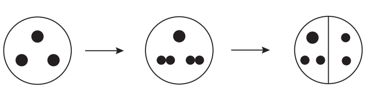
Figure 12.1. Externally excited quarks split in pairs, forming new hadrons.

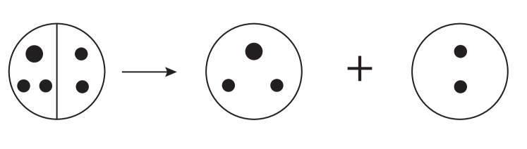
Figure 12.2. Two hadrons being push apart after splitting.

(2) When the quarks in a hadron is split forming two or more hadrons, the strong interaction between the two newly formed hadrons follow immediately the strong interaction potential (11.23) for nucleons/hadrons. As these two new hadrons are too close, the strong nuclear force with potential (11.23) is repelling, causing decay.

(3) Quark splitting appears to occur in pairs, i.e. evenness or oddness of the total number of quarks is invariant in a decay process.

13. Stability of Matter

Based on the theory presented in the previous sections, the structure and stability of matter can be understood in four different scales from the largest cosmos to the smallest elementary particles as follows:

Stars, galaxies and cosmos. Gravity plays the most important role for the structure and its formation of large scale stars, galaxies and cosmos. It is the new gravitational force formula (11.14) established in [15] that shows that gravity is both attracting (Newton and dark matter) for the scale smaller than 10 million light years, and repelling (dark energy) for scale greater than 10 million light years. The largest scale repelling of gravity avoids an eventual collapsing of all galaxies. The attraction of gravity in a relatively smaller scale enables the formation of stars and galaxies.

The dual field $\varphi$ in the gravitational field equations (11.10) causes the repelling of gravity in the largest scale. It is shown in [15] that the dual $\varphi$ vanishes if the matter in the universe is uniformly distributed. In summary, it is the interaction between the gravitational field $\{g_{\mu\nu}\}$ and the dual field $\varphi$ that maintains the large scale structure of the universe.

Atomic and molecular level. Atoms and molecules are held together by Coulomb attracting force. The reasons why atoms do not collapse are mainly due to 1) the energy levels of electrons preventing electrons from collapsing to the nuclear, and 2) the Pauli principle for the stability of bulk matter; see among others [12].

Nucleons/hadron level. By (11.22), the strong interacting force between two quarks is repelling as the distance between them is small avoiding the collapsing quarks together, and is attracting holding them together and forming a hadron as the distance increases. In the hadron level, by (11.23), the strong acting also are repelling when two hadrons are close (less than $10^{-13}$cm), again avoiding the collapsing of hadrons. When the distance between two hadrons increases (about $10^{-13}-10^{-12}$cm), the strong attracting force takes place binding hadrons together forming a nuclear. Then by (11.24), when the distance between two molecules or atoms is less than $10^{-7}$cm, the strong repelling force induces the van der Waals repelling force.

Lepton and quark level. In this level, the acting force is the weak force (11.29). Again the short distance repelling avoids collapsing, and followed by attracting weak force forming a lepton or a quark.

In summary, all four forces display both attracting and repelling hold matter/particle together and avoiding collapsing at the same time. This is the essence of the stability of matter in the universe from the smallest elementary particles to largest galaxies in the universe. Also, the energy levels for leptons and hadrons classifies all leptons and hadrons with electron and proton being the smallest energy level elementary particles.

14. Conclusions of Part 1

The main objective of Part 1 is to drive a unified field model coupling four interactions, based on the principle of interaction dynamics (PID) and the principle of representation invariance (PID). Intuitively, PID takes the variation of the action functional under energy-momentum conservation constraint. PRI requires that physical laws be independent of representations of the gauge groups. One important outcome of this unified field model is a natural duality between the interacting fields $(g,A,W^{a},S^{k})$, corresponding to graviton, photon, intermediate vector bosons $W^{\pm}$ and $Z$ and gluons, and the adjoint bosonic fields $(\Phi_{\mu},\phi^{E},\phi^{a}_{w},\phi^{k}_{s})$. This duality predicts two Higgs particles of similar mass with one due to weak interaction and the other due to strong interaction. PID and PRI can be applied directly to individual interactions, leading to 1) modified Einstein equations, giving rise to a unified theory for dark matter and dark energy, 2) three levels of strong interaction potentials for quark, nucleon/hadron, and atom respectively, and 3) a weak interaction potential. These potential/force formulas offer a clear mechanism for both quark confinement and asymptotic freedom—a longstanding problem in particle physics. Also, we intend to offer our view on such questions as why our universe is as it is, by introducing energy levels for leptons and quarks as well as for hadrons, and by exploring essential characteristics of the potential/force formulas.

Part II Weakton Model of Elementary Particles and Decay Mechanisms

15. Introduction

The matter in the universe is made up of a number of fundamental constituents. The current knowledge of elementary particles shows that all forms of matter are made up of 6 leptons and 6 quarks, and their antiparticles. The basic laws governing the dynamical behavior of these elementary particles are the laws for the four interactions/forces: the electromagnetism, the gravity, the weak and strong interactions. Great achievements and insights have been made for last 100 years or so on the understanding of the structure of subatomic particles and on the fundamental laws for the four interactions; see among many others [7, 5, 11, 25, 21].

However, there are still many longstanding open questions and challenges. Here are a few fundamental questions which are certainly related to the deepest secret of our universe:

• What is the origin of four forces?

• Why do leptons not participate in strong interactions?

• What is the origin of mass?

• What is the mechanism of subatomic decays and reactions?

• Why can massless photons produce massive particles? Or in general, why can lepton and anti-lepton pairs produce hadron pairs?

• Are leptons and quarks true elementary particles? Do leptons and quarks have interior structure?

• Why are there more matters than anti-matters? This is the classical baryon asymmetry problem.

• What are the strong and weak force formulas?

• Why, in the same spatial scale, do strong and weak interactions exhibit both repelling and attraction?

• Why are the weak and strong interactions short-ranged, and what are the ranges of the four interactions?

• What is the mechanism of quark confinement?

• What is the mechanism of bremsstrahlung?

The main objectives of Part 2 of this article are 1) to study the mechanism of subatomic decays, 2) to propose a weakton model of elementary particles, and 3) to explain the above questions Q₁–Q₁₂. We proceed as follows.

1. The starting point of the study is the puzzling decay and reaction behavior of subatomic particles. For example, the electron radiations and the electron-positron annihilation into photons or quark-antiquark pair clearly shows that there must be interior structure of electrons, and the constituents of an electron contribute to the making of photon or the quark in the hadrons formed in the process. In fact, all sub-atomic decays and reactions show clearly the following conclusion:

(15.1) There must be interior structure of charged leptons, quarks and mediators.

2. The above conclusion motivates us to propose a model for sub-lepton, sub-quark, and sub-mediators. It is clear that any such model should obey four basic requirements.

The first is the mass generation mechanism. Namely, the model should lead to consistency of masses for both elementary particles, which we call weaktons to be introduced below, and composite particles (the quarks, leptons and mediators). Since the mediators, the photon $\gamma$ and the eight gluons $g^{k}$ ($k=1,\cdots,8$), are all massless, a natural requirement is that

(15.2) the proposed elementary particles—weaktons— are massless.

Namely, these proposed elementary particles must have zero rest mass.

The second requirement for the model is the consistency of quantum numbers for both elementary and composite particles. The third requirement is the exclusion of nonrealistic compositions of the elementary particles, and the fourth requirement is the weakton confinement.

3. Careful examinations of these requirements and subatomic decays/reactions lead us to propose six elementary particles, which we call weaktons, and their anti-particles:

(15.3) $$w^{*}, w_{1}, w_{2}, \nu_{e}, \nu_{\mu}, \nu_{\tau},$$

$$\bar{w}^{*}, \bar{w}_{1}, \bar{w}_{2}, \bar{\nu}_{e}, \bar{\nu}_{\mu}, \bar{\nu}_{\tau},$$

where $\nu_{e},\nu_{\mu},\nu_{\tau}$ are the three generation neutrinos, and $w^{*},w_{1},w_{2}$ are three new particles, which we call $w$-weaktons. These are massless, spin-$\frac{1}{2}$ particles with one unit of weak charge $g_{w}$. Both $w^{\ast}$ and $\bar{w}^{\ast}$ are the only weaktons carrying strong charge $g_{s}$.

With these weaktons at our disposal, the weakton constituents of charged leptons and quarks are then given as follows:

(15.4) $$e=\nu_{e}w_{1}w_{2}, \mu=\nu_{\mu}w_{1}w_{2}, \tau=\nu_{\tau}w_{1}w_{2},$$

$$u=w^{*}w_{1}\bar{w}_{1}, c=w^{*}w_{2}\bar{w}_{2}, t=w^{*}w_{2}\bar{w}_{2},$$

$$d=w^{*}w_{1}w_{2}, s=w^{*}w_{1}w_{2}, b=w^{*}w_{1}w_{2},$$

where $c,t$ and $d,s,b$ are distinguished by the spin arrangements; see (18.6) and (18.7).

4. Using the duality given in the unified field theory for four interactions, the mediators of strong, weak and electromagnetic interactions include the photon $\gamma$, the vector bosons $W^{\pm}$ and $Z$, and the gluons $g^{k}$, together with their dual fields $\phi_{\gamma}$, $\phi^{\pm}_{W}$, $\phi_{Z}^{0}$, and $\phi_{g}^{k}$. The constituents of these mediators are given by

(15.5) $$\gamma=\cos\theta_{w}w_{1}\bar{w}_{1}-\sin\theta_{w}w_{2}\bar{w}_{2}\ (\upuparrows,\downdownarrows),$$

$$Z^{0}=\cos\theta_{w}w_{2}\bar{w}_{2}+\sin\theta_{w}w_{1}\bar{w}_{1}\ (\upuparrows,\downdownarrows),$$

$$W^{-}=w_{1}w_{2}(\upuparrows,\downdownarrows),$$

$$W^{+}=\bar{w}_{1}\bar{w}_{2}(\upuparrows,\downdownarrows),$$

$$g^{k}=w^{*}\bar{w}^{*}(\upuparrows,\downdownarrows),\ \ \ \ k=\text{\rm color index},$$

and the dual bosons:

(15.6) $$\phi_{\gamma}=\cos\theta_{w}w_{1}\bar{w}_{1}-\sin\theta_{w}w_{2}\bar{w}_{2}(\uparrow\downarrow,\downarrow\uparrow),$$

$$\phi^{0}_{Z}=\cos\theta_{w}w_{2}\bar{w}_{2}+\sin\theta_{w}w_{1}\bar{w}_{1}(\uparrow\downarrow,\downarrow\uparrow),$$

$$\phi^{-}_{W}=w_{1}w_{2}(\uparrow\downarrow,\downarrow\uparrow),$$

$$\phi^{+}_{W}=\bar{w}_{1}\bar{w}_{2}(\uparrow\downarrow,\downarrow\uparrow),$$

$$\phi^{k}_{g}=w^{*}\bar{w}^{*}(\uparrow\downarrow,\downarrow\uparrow),$$

where $\theta_{w}\cong 28.76^{\circ}$ is the Weinberg angle.

Remarkably, both the spin-1 mediators in (15.5) and the spin-0 dual mediators in (15.6) have the same weakton constituents, differing only by their spin arrangements. The spin arrangements clearly demonstrate that there must be spin-0 particles with the same weakton constituents as the mediators in (15.5). Consequently, there must be dual mediators with spin-0. This observation clearly supports the unified field model presented in [17] and in Part I of this article. Conversely, the existence of the dual mediators makes the weakton constituents perfectly fit.

5. Also, a careful examination of weakton constituents predicts the existence of an additional mediator, which we call the $\nu$-mediator:

(15.7) $$\phi^{0}_{\nu}=\sum\limits_{l}\alpha_{l}\nu_{l}\bar{\nu}_{l}(\downarrow\uparrow),\ \ \ \ \sum\limits_{l}\alpha^{2}_{l}=1,$$

taking into consideration of neutrino oscillations. When examining decays and reactions of sub-atomic particles, it is apparent for us to predict the existence of this mediator.

6. One important conclusion of the aforementioned weakton model is that all particles—both matter particles and mediators—are made up of massless weaktons. A fundamental question is how the mass of a massive composite particle is generated. In fact, based on the Einstein formulas:

(15.8) $$\frac{d}{dt}\vec{P}=\sqrt{1-\frac{v^{2}}{c^{2}}}\vec{F},\qquad m=\sqrt{1-\frac{v^{2}}{c^{2}}}\frac{E}{c^{2}},$$

we observe that a particle with an intrinsic energy $E$ has zero mass $m=0$ if it moves in the speed of light $v=c$, and possess nonzero mass if it moves with a velocity $v<c$. Hence by this mass generation mechanism, for a composite particle, the constituent massless weaktons can decelerate by the weak force, yielding a massive particle.

In principle, when calculating the mass of the composite particle, one should also consider the bounding and repelling energies of the weaktons, each of which can be very large. Fortunately, the constituent weaktons are moving in the “asymptotically-free” shell region of weak interactions as indicated by the weak interaction potential/force formulas, so that the bounding and repelling contributions to the mass are mostly canceled out. Namely, the mass of a composite particle is due mainly to the dynamic behavior of the constituent weaktons.

7. As we mentioned earlier, one requirement for the weakton model is the consistency of quantum numbers for both elementary particles and composite particles. In fact, the weakton model obeys a number of quantum rules, which can be used to exclude unrealistic combinations of weaktons. The following rules are introduced for this purpose:

• Weak color neutral rule: each weakton is endowed with a weak color quantum number, and all weakton composite particles must be weak color neutral.

• $BL=0,L_{i}L_{j}=0\ (i\neq j)$, where $B$ is the baryon number and $L$ is the lepton number.

• $L+Q_{e}=0$ if $L\neq 0$ and $|B+Q_{e}|\leq 1$ if $B\neq 0$.

• Angular Momentum Rule: Only the fermions with spin $s=\frac{1}{2}$ can rotate around a center with zero moment of force. The particles with $s\neq\frac{1}{2}$ will move in a straight line unless there is a nonzero moment of force present.

  The angular momentum is a consequence of the Dirac equations, and it is due to this rule that there are no spin-3/2 quarks.

8. Remarkably, the weakton model offers a perfect explanation for all sub-atomic decays. In particular, all decays are achieved by 1) exchanging weaktons and consequently exchanging newly formed quarks, producing new composite particles, and 2) separating the new composite particles by weak and/or strong forces.

One aspect of this decay mechanism is that we know now the precise constituents of particles involved in all decays/reactions both before and after the reaction. It is therefore believed that the new decay mechanism provides clear new insights for both experimental and theoretical studies.

9. The weakton theory, together with the unified field theory developed in [17] and in Part 1 of this article, provides sound explanations and new viewpoints for the twelve fundamental questions given at the beginning of the Introduction.

We end this Introduction by mentioning that there have been numerous studies on sub-quark and sub-lepton models; see among others [20, 2, 23, 8]

Part 2 of this article was first appeared as an independent preprint [18], and is organized as follows. A brief introduction to the current understanding of elementary particles is given in Section 16, focusing on 1) the constituents of subatomic particles, and 2) decays. Section 17 addresses a few theoretical foundations needed for introducing the weakton model, which is then introduced in Section 18. All decays are then perfectly explained using the weakton model in Section 19. An application of the weakton model to bremsstrahlung is given in Section 20. Section 21 summaries conclusions of Part 2, focusing on answers and explanations to the above 12 open questions.

16. Current Knowledge of Elementary Particles

The current view on subatomic particles classifies all particles into two basic classes, bosons and fermions:

$$\text{\rm bosons = integral spin particles},$$

fermions = fractional spin particles.

However, based on their properties and laws in Nature, all particles are currently classified into four types:

leptons, quarks, mediators, hadrons.

Hereafter we recapitulate the definitions and the quantum characterizations of these particles.

16.1. Leptons

Leptons are fermions which do not participate in strong interaction, and have three generations with two in each generation:

$$\left(\begin{matrix}e\\ \nu_{e}\end{matrix}\right),\qquad\left(\begin{matrix}\mu\\ \nu_{\mu}\end{matrix}\right),\qquad\left(\begin{matrix}\tau\\ \nu_{\tau}\end{matrix}\right),$$

where $e,\mu,\tau$ are the electron, the muon, the tau, and $\nu_{e},\nu_{\mu},\nu_{\tau}$ are the $e$ neutrino, the $\mu$ neutrino, the $\tau$ neutrino. Together with antiparticles, there are total 12 leptons:

particles: $$(e^{-},\nu_{e}),\ (\mu^{-},\nu_{\mu}),\ (\tau^{-},\nu_{\tau}),$$

antiparticles: $$(e^{+},\bar{\nu}_{e}),\ (\mu^{+},\bar{\nu}_{\mu}),\ (\tau^{+},\bar{\nu}_{\tau}).$$

The quantum numbers of leptons include the mass $m$, the charge $Q$, the lifetime $\tau$, the spin $J$, the $e$-lepton number $L_{e}$, the $\mu$-lepton number $L_{\mu}$, and the $\tau$-lepton number $L_{\tau}$. Table 1 lists typical values of these quantum numbers, where the mass is in Me$V/c^{2}$, lifetime is in seconds, and the charge is in the unit of proton charge. Also, we remark that the left-hand property of neutrinos is represented by $J=-\frac{1}{2}$ for $\nu$, and $J=+\frac{1}{2}$ for $\bar{\nu}$.

Table 1. Leptons

lepton	$M$	$Q$	$J$	$L_{e}$	$L_{\mu}$	$L_{\tau}$	$\tau$
$e^{-}$	0.51	-1	$\pm{1}/{2}$	1	0	0	$\infty$
$\nu_{e}$	0	0	$-{1}/{2}$	1	0	0	$\infty$
$e^{+}$	0.51	+1	$\pm 1/2$	-1	0	0
$\bar{\nu}_{e}$	0	0	$+1/2$	-1	0	0	$\infty$
$\mu^{-}$	105.7	-1	$\pm 1/2$	0	1	0	$2.2\times 10^{-6}$
$\nu_{\mu}$	0	0	$-1/2$	0	1	0	$\infty$
$\mu^{+}$	105.7	+1	$\pm 1/2$	0	-1	0
$\bar{\nu}_{\mu}$	0	0	$+1/2$	0	-1	0	$\infty$
$\tau^{-}$	1777	-1	$\pm 1/2$	0	0	1	$3\times 10^{-13}$
$\nu_{\tau}$	0	0	$-1/2$	0	0	1	$\infty$
$\tau^{+}$	1777	+1	$\pm 1/2$	0	0	-1
$\bar{\nu}_{\tau}$	0	0	$+1/2$	0	0	-1	$\infty$

16.2. Quarks

Based on the Standard Model, there are three generations of quarks containing 12 particles, which participate in all interactions:

quarks: $$(u,d),\ (c,s),\ (t,b),$$

antiquarks: $$(\bar{u},\bar{d}),\ (\bar{c},\bar{s}),\ (\bar{t},\bar{b}).$$

The celebrated quark model assets that three quarks are bounded together to form a baryon, and a pair of quark and antiquark are bounded to form a meson. Quarks are confined in hadrons, and no free quarks have been found in Nature. This phenomena is called quark confinement, which can be very well explained using the three levels of strong interaction potentials derived using the unified field theory developed recently in [17] and in Part 1 of this article; see discussions in Section 17.4.

The quantum numbers of quarks include the mass $m$, the charge $Q$, the baryon number $B$, the spin $J$, the strange number $S$, the isospin $I$ and its third component $I_{3}$, the supercharge $Y$, and the parity $P$. These quantum numbers are listed in Table 2.

Table 2. Quarks

Quarks	$m$	$Q$	$J$	$B$	$S$	$Y$	$I$	$I_{3}$	$P$
$u$	3	$2/3$	$\pm 1/2$	$1/3$	0	$1/3$	$1/2$	$+1/2$	+1
$d$	7	$-1/3$	$\pm 1/2$	$1/3$	0	$1/3$	$1/2$	$-1/2$	+1
$c$	1200	$2/3$	$\pm 1/2$	$1/3$	0	$1/3$	0	0	+1
$s$	120	$-1/3$	$\pm 1/2$	$1/3$	-1	$-2/3$	0	0	+1
$t$	$1.7\times 10^{5}$	$2/3$	$\pm 1/2$	$1/3$	0	$1/3$	0	0	+1
$b$	4300	$-1/3$	$\pm 1/2$	$1/3$	0	$1/3$	0	0	+1
$\bar{u}$	3	$-2/3$	$\pm 1/2$	$-1/3$	0	$-1/3$	$1/2$	$-1/2$	-1
$\bar{d}$	7	$1/3$	$\pm 1/2$	$-1/3$	0	$-1/3$	$1/2$	$+1/2$	-1
$\bar{c}$	1200	$-2/3$	$\pm 1/2$	$-1/3$	0	$-1/3$	0	0	-1
$\bar{s}$	120	$1/3$	$\pm 1/2$	$-1/3$	+1	$2/3$	0	0	-1
$\bar{t}$	$1.7\times 10^{5}$	$-2/3$	$\pm 1/2$	$-1/3$	0	$-1/3$	0	0	-1
$\bar{b}$	4300	$1/3$	$\pm 1/2$	$-1/3$	0	$-1/3$	0	0	-1

16.3. Mediators

The standard model shows that associated with each interaction is a class of mediators. Namely, there are four classes of mediators:

Gravitation: $$\text{\rm graviton}\ g_{G},$$

Electromagnetism: $$\text{\rm photon}\ \gamma,$$

Weak interaction: $$\text{\rm vector meson}\ W^{\pm},Z^{0},$$

Strong interaction: $$\text{\rm gluons}\ g^{k}\ (1\leq k\leq 8).$$

The quantum numbers of these mediators include the mass $m$, the charge $Q$, the spin $J$, and the lifetime $\tau$, listed in Table 3.

Table 3. Interaction Mediators

Interaction	Mediator	$m$	$Q$	$J$	$\tau$
Gravitation	$g_{G}$	0	0	2	$\infty$
Electromagnetic	$\gamma$	0	0	1	$\infty$
	$W^{+}$	$8\times 10^{4}$	+1	1	$3\times 10^{-25}$
Weak	$W^{-}$	$8\times 10^{4}$	-1	1	$3\times 10^{-25}$
	$Z^{0}$	$9\times 10^{4}$	0	1	$2.6\times 10^{-25}$
Strong	$g^{k}(1\leq k\leq 8)$	0	0	1	$\infty$

With the unified field theory developed in [17] and in Part 1 of this article, we have obtained a natural duality between the interacting fields $\{g_{\mu\nu},A_{\mu},W^{a}_{\mu},S^{k}_{\mu}\}$ and their dual field $\{\Phi^{G}_{\mu},\phi_{E},\phi^{a}_{w},\phi^{k}_{s}\}$:

$$\{g_{\mu\nu}\} \longleftrightarrow \Phi^{G}_{\mu},$$

$$A_{\mu} \longleftrightarrow \phi_{E},$$

$$\{W^{a}_{\mu}\} \longleftrightarrow \{\phi^{a}_{w}\},$$

$$\{S^{k}_{\mu}\} \longleftrightarrow \{\phi^{k}_{s}\}.$$

This duality leads to four classes of new dual bosonic mediators:

(16.1) $$\text{\rm graviton}\ g_{G} \longleftrightarrow \text{\rm vector boson}\ \Phi^{G},$$

$$\text{\rm photon}\ \gamma \longleftrightarrow \text{\rm scalar boson}\ \phi_{\gamma},$$

$$\text{\rm vector bosons}\ W^{\pm},Z \longleftrightarrow \text{\rm scalar bosons}\ \phi^{\pm}_{W},\phi^{0}_{Z},$$

$$\text{\rm gluons}\ g^{k}\ (1\leq k\leq 8) \longleftrightarrow \text{\rm scalar bosons}\ \phi^{k}_{g}\ (1\leq k\leq 8)$$

These dual mediators are crucial not only for the weak and strong potential/force formulas given in the next section, but also for the weakton model introduced in this article. In addition, the dual vector field $\Phi^{G}$ gives rise to a unified theory for dark matter and dark energy [15].

The quantum numbers of these dual mediators are given as follows:

(16.2) $$\Phi^{G}: m=0, J=1, Q=0, \tau=\infty,$$

$$\phi_{e}: m=0, J=0, Q=0, \tau=\infty,$$

$$\phi^{\pm}_{W}(\text{\rm Higgs}): m\sim 10^{5}, J=0, Q=\pm 1, \tau\sim 10^{-21}s,$$

$$\phi^{0}_{Z}(\text{\rm Higgs}): m\sim 1.25\times 10^{5}, J=0, Q=0, \tau\sim 10^{-21}s,$$

$$\phi^{k}_{g}: m=?, J=0, Q=0, \tau=?.$$

16.4. Hadrons

Hadrons are classified into two types: baryons and mesons. Baryons are fermions and mesons are bosons, which are all made up of quarks:

$$\text{\rm Baryons}\ =q_{i}q_{j}q_{k}, \text{\rm mesons}\ =q_{i}\bar{q}_{j},$$

where $q_{k}=\{u,d,c,s,t,b\}$. The quark constituents of main hadrons are listed as follows:

• Baryons $(J=\frac{1}{2}):p,n,\Lambda,\Sigma^{\pm},\Sigma^{0},\Xi^{0},\Xi^{-}$.

  (16.3) $$p(uud), n(udd), \Lambda(s(du-ud)/\sqrt{2}),$$

  $$\Sigma^{+}(uus), \Sigma^{-}(dds), \Sigma^{0}(s(du+ud)/\sqrt{2}),$$

  $$\Xi^{-}(uss), \Xi^{0}(dss).$$

• Baryons $(J=\frac{3}{2}):\Delta^{++},\Delta^{\pm},\Delta^{0},\Sigma^{*\pm},\Sigma^{*0},\Xi^{*0},\Xi^{*-},\Omega^{-}$.

  (16.4) $$\Delta^{++}(uuu), \Delta^{+}(uud), \Delta^{-}(ddd), \Delta^{0}(udd),$$

  $$\Sigma^{*+}(uus), \Sigma^{*-}(dds), \Sigma^{*0}(uds),$$

  $$\Xi^{*0}(uss), \Xi^{*-}(dss), \Omega^{-}(sss).$$

• Mesons $(J=0):\pi^{\pm},\pi^{0},K^{\pm},K^{0},\bar{K}^{0},\eta$,

  (16.5) $$\pi^{+}(u\bar{d}), \pi^{-}(\bar{u}d), \pi^{0}((u\bar{u}-d\bar{d})/\sqrt{2}),$$

  $$K^{+}(u\bar{s}), K^{-}(\bar{u}s), K^{0}((d\bar{s}), \bar{K}^{0}(\bar{d}s),$$

  $$\eta((u\bar{u}+d\bar{d}-2s\bar{s})/\sqrt{6}).$$

• Mesons $(J=1):\rho^{\pm},\rho^{0},K^{*\pm},K^{*0},\bar{K}^{*0},\omega,\psi,\Upsilon$,

  (16.6) $$\rho^{+}(u\bar{d}), \rho^{-}(\bar{u}d), \rho^{0}((u\bar{u}-d\bar{d})/\sqrt{2}),$$

  $$K^{*+}(u\bar{s}), K^{*-}(\bar{u}s), K^{*0}(\bar{d}s), \bar{K}^{*0}(\bar{d}s),$$

  $$\omega((u\bar{u}+d\bar{d})/\sqrt{2}), \psi(c\bar{c}), \Upsilon(b\bar{b}).$$

16.5. Principal decays

Decays are the main dynamic behavior for sub-atomic particles, and reveal the interior structure of particles. We now list some principal decay forms.

• Lepton decays:

  $$\mu^{-}\rightarrow e^{-}+\bar{\nu}_{e}+\nu_{\mu},$$

  $$\mu^{+}\rightarrow e^{+}+\nu_{e}+\bar{\nu}_{\mu},$$

  $$\tau^{-}\rightarrow e^{-}+\bar{\nu}_{e}+\nu_{\tau},$$

  $$\tau^{-}\rightarrow\mu^{-}+\bar{\nu}_{\mu}+\nu_{\tau},$$

  $$\tau^{-}\rightarrow\pi^{-}+\nu_{\tau},$$

  $$\tau^{-}\rightarrow\rho^{-}+\nu_{\tau},$$

  $$\tau^{-}\rightarrow K^{-}+\nu_{\tau}.$$

• Quark decays:

  $$d\rightarrow u+e^{-}+\bar{\nu}_{e},$$

  $$s\rightarrow u+e^{-}+\bar{\nu}_{e},$$

  $$s\rightarrow d+g+\gamma (g\ \text{\rm the gluons}),$$

  $$c\rightarrow d+\bar{s}+u,$$

• Mediator decays:

  $$2\gamma\rightarrow e^{+}+e^{-},\ q\bar{q},$$

  $$W^{+}\rightarrow e^{+}+\nu_{e},\ \mu^{+}+\nu_{\mu},\ \tau^{+}+\nu_{\tau},$$

  $$W^{-}\rightarrow e^{-}+\bar{\nu}_{e},\ \mu^{-}+\bar{\nu}_{\mu},\ \tau^{-}+\bar{\nu}_{\tau},$$

  $$Z^{0}\rightarrow e^{+}+e^{-},\ \mu^{+}+\mu^{-},\ \tau^{+}+\tau^{-},\ q\bar{q}.$$

• Baryon decays:

  $$n\rightarrow p+e^{-}+\bar{\nu}_{e},$$

  $$\Lambda\rightarrow p+\pi^{-},\ n+\pi^{0},$$

  $$\Sigma^{+}\rightarrow p+\pi^{0},\ n+\pi^{+},$$

  $$\Sigma^{0}\rightarrow\Lambda+\gamma,\ \Sigma^{-}\rightarrow n+\pi^{-},$$

  $$\Xi^{0}\rightarrow\Lambda+\pi^{0},\ \Xi^{-}\rightarrow\Lambda+\pi^{-},$$

  $$\Delta^{++}\rightarrow p+\pi^{+},\ \Delta^{+}\rightarrow p+\pi^{0},$$

  $$\Delta^{0}\rightarrow n+\pi^{0},\ \Delta^{-}\rightarrow n+\pi^{-},$$

  $$\Sigma^{*\pm}\rightarrow\Sigma^{\pm}+\pi^{0},\ \Xi^{*0}\rightarrow\Sigma^{0}+\pi^{0},$$

  $$\Xi^{*0}\rightarrow\Xi^{0}+\pi^{0},\ \Xi^{*-}\rightarrow\Xi^{-}+\pi^{0}.$$

• Meson decays:

  $$\pi^{+}\rightarrow\mu^{+}+\nu_{\mu},\ \ \ \ \pi^{0}\rightarrow 2\gamma,$$

  $$\pi^{-}\rightarrow\mu^{-}+\bar{\nu}_{\mu},$$

  $$K^{+}\rightarrow\mu^{+}+\nu_{\mu},\ \pi^{+}+\pi^{0},\ \pi^{+}+\pi^{+}+\pi^{-},$$

  $$K^{-}\rightarrow\mu^{-}+\bar{\nu}_{\mu},\ \pi^{-}+\pi^{0},\ \pi^{-}+\pi^{+}+\pi^{-},$$

  $$K^{0}\rightarrow\pi^{+}+e^{-}+\bar{\nu}_{e},\ \pi^{+}+\pi^{-},\ \pi^{+}+\pi^{-}+\pi^{0},$$

  $$\eta\rightarrow 2\gamma,\ \pi^{+}+\pi^{-}+\pi^{0},$$

  $$\rho^{\pm}\rightarrow\pi^{0},\ \rho^{0}\rightarrow\pi^{+}+\pi^{-},$$

  $$K^{*\pm}\rightarrow K^{\pm}+\pi^{0},\ K^{*0}\rightarrow K^{0}+\pi^{0},$$

  $$\omega\rightarrow\pi^{0}+\gamma,\ \pi^{+}+\pi^{-}+\pi^{0},$$

  $$\psi\rightarrow e^{+}+e^{-},\ \mu^{+}+\mu^{-},$$

  $$\Upsilon\rightarrow e^{+}+e^{-},\ \mu^{+}+\mu^{-},\ \tau^{+}+\tau^{-}.$$

17. Theoretical Foundations for the Weakton Model

17.1. Angular momentum rule

It is known that the dynamic behavior of a particle is described by the Dirac equations:

(17.1) $$i\hbar\frac{\partial\psi}{\partial t}=H\psi,\ \ \ \ \psi=(\psi_{1},\psi_{2},\psi_{3},\psi_{4})^{T}$$

where $H$ is the Hamiltonian

(17.2) $$H=-i\hbar c(\alpha^{k}\partial_{k})+mc^{2}\alpha^{0}+V(x),$$

$V$ is the potential energy, and $\alpha^{0},\alpha^{k}\ (1\leq k\leq 3)$ are the Dirac matrices

$$\alpha^{0}=\left(\begin{array}[]{cccc}1&&&0\\ &1\\ &&-1\\ 0&&&-1\end{array}\right),\ \ \ \ \alpha^{1}=\left(\begin{array}[]{cccc}0&0&0&1\\ 0&0&1&0\\ 0&1&0&0\\ 1&0&0&0\end{array}\right),$$

$$\alpha^{2}=\left(\begin{array}[]{cccc}0&0&0&-i\\ 0&0&i&0\\ 0&-i&0&0\\ i&0&0&0\end{array}\right),\ \ \ \ \alpha^{3}=\left(\begin{array}[]{cccc}0&0&1&0\\ 0&0&0&-1\\ 1&0&0&0\\ 0&-1&0&0\end{array}\right).$$

By the conservation laws in relativistic quantum mechanics, if a Hermitian operator $L$ commutes with $H$ in (17.2):

$$LH=HL,$$

then the physical quantity $L$ is conservative.

Consider the total angular momentum $\vec{J}$ of a particle given by

$$\vec{J}=\vec{L}+s\hbar\vec{S},$$

where $L$ is the orbital angular momentum

$$\vec{L}=\vec{r}\times\vec{p},\ \ \ \ \vec{p}=-i\hbar\nabla,$$

$\vec{S}$ is the spin

$$\vec{S}=(S_{1},S_{2},S_{3}),\ S_{k}=\left(\begin{array}[]{cc}\sigma_{k}&0\\ 0&\sigma_{k}\end{array}\right),$$

and $\sigma_{k}\ (1\leq k\leq 3)$ are the Pauli matrices.

We know that for $H$ in (17.2)

(17.5) $$\vec{J}_{{1}/{2}}=\vec{L}+\frac{1}{2}\hbar\vec{S} \text{\rm commutes with}\ H,$$

$$\vec{J}_{s}=\vec{L}+s\hbar\vec{S} \text{\rm does not commute with}\ H\ \text{\rm for}\ s\neq{1}/{2}\text{ in general}.$$

Also, we know that

(17.6) $$s\hbar\vec{S}\ \text{\rm commutes with }\ H\ \text{\rm with straight line motion for any}\ s.$$

The properties in (17.5) imply that only particles with spin $s=\frac{1}{2}$ can make a rotational motion in a center field with free moment of force. However, (17.6) implies that the particles with $s\neq\frac{1}{2}$ will move in a straight line, i.e. $\vec{L}=0$, unless they are in a field with nonzero moment of force.

In summary, we have derived the following angular momentum rule for sub-atomic particle motion, which is important for our weakton model established in the next section.

Angular Momentum Rule: Only the fermions with spin $s=\frac{1}{2}$ can rotate around a center with zero moment of force. The particles with $s\neq\frac{1}{2}$ will move on a straight line unless there is a nonzero moment of force present.

For example, the particles bounded in a ball rotating around the center, as shown in Figure 17.1, must be fermions with $s=\frac{1}{2}$.

Figure 17.1. (a) Two particles $A,B$ rotate around the center $O$; (b) three particle $A,B,C$ rotate around the center $O$.

17.2. Mass generation mechanism

For a particle moving with velocity $v$, its mass and energy $E$ obey the Einstein relation

(17.7) $$E={mc^{2}}\Big{/}{\sqrt{1-\frac{v^{2}}{c^{2}}}}.$$

Usually, we regard $m$ as a static mass which is fixed, and energy $E$ is a function of velocity $v$.

Now, taking an opposite viewpoint, we regard energy $E$ as fixed, and mass $m$ is a function of velocity $v$, i.e. the relation (17.7) is rewritten as

(17.8) $$m=\sqrt{1-\frac{v^{2}}{c^{2}}}\frac{E}{c^{2}}.$$

Thus, (17.8) means that a particle with an intrinsic energy $E$ has zero mass $m=0$ if it moves at the speed of light $v=c$, and will possess nonzero mass if it moves with a velocity $v<c$. All particles including photons can only travel at the speed sufficiently close to the speed of light. Based on this viewpoint, we can think that if a particle moving at the speed of light (approximately) is decelerated by an interaction field, obeying

$$\frac{d\vec{P}}{dt}=\sqrt{1-\frac{v^{2}}{c^{2}}}\vec{F},$$

then this massless particle will generate mass at the instant. In particular, by this mass generation mechanism, several massless particles can yield a massive particle if they are bounded in a small ball, and rotate at velocities less than the speed of light.

From this mass generation mechanism, we can also understand the neutrino oscillation phenomena. Experiments show that each of the three neutrinos $\nu_{e},\nu_{\tau},\nu_{\mu}$ can transform from one to another, although the experiments illustrate that neutrinos propagate at the speed of light. This oscillation means that they generate masses at the instant of transformation. This can be viewed as the neutrinos decelerate at the instant when they undergo the transformation/oscillation, generating instantaneous masses, and after the transformation, they return to the usual dynamic behavior–moving at the speed of light with zero masses. In other words, by the mass generation mechanism, we can assert that neutrinos have no static masses, and their oscillations give rise to instantaneous masses.

17.3. Interaction charges

In the unified field model developed in [17] and in Part 1 of this article, we derived that both weak and strong interactions possess charges, as for gravity and electromagnetism:

(17.9) gravitation: $$\text{\rm mass charge}\ m$$

electromagnetism: $$\text{\rm electric charge}\ e,$$

weak interaction: $$\text{\rm weak charge}\ g_{w},$$

strong interaction: $$\text{\rm strong charge}\ g_{s}.$$

If $\Phi$ is a charge potential corresponding to an interaction, then the interacting force generated by its charge $\mathfrak{C}$ is given by

(17.10) $$F=-\mathfrak{C}\nabla\Phi,$$

where $\nabla$ is the spatial gradient operator.

The charges in (17.9) possess the physical properties:

• Electric charges $Q_{e}$, weak charges $Q_{w}$, strong charges $Q_{s}$ are conservative. The energy is a conserved quantity, but the mass $M$ is not a conserved quantity due to the mass generation mechanism as mentioned earlier.

• There is no interacting force between two particles without common charges. For example, if a particle A possesses no strong charge, then there is no strong interacting force between $A$ and any other particles.

• Only the electric charge $Q_{e}$ can take both positive and negative values, and other charges can take only nonnegative values.

• Only the mass charge is continuous, and the others are discrete, taking discrete values.

• We emphasize that the continuity of mass is the main obstruction for quantizing the gravitational field, and it might be essential that gravity cannot be quantized.

17.4. Strong interaction potentials

Three levels of strong interacting potentials are derived in Part 1 of this article using the field equations, and they are called the quark potential $S_{q}$, the hadron potential $S_{h}$, and the atom/molecule potential $S_{a}$:

(17.11) $$S_{q}=g_{s}\left[\frac{1}{r}-\frac{Bk^{2}_{0}}{\rho_{0}}e^{-k_{0}r}\varphi(r)\right],$$

(17.12) $$S_{h}=N_{0}\left(\frac{\rho_{0}}{\rho_{1}}\right)^{3}g_{s}\left[\frac{1}{r}-\frac{B_{1}}{\rho_{1}}k^{2}_{1}e^{-k_{1}r}\varphi(r)\right],$$

(17.13) $$S_{a}=3N_{1}\left(\frac{\rho_{0}}{\rho_{1}}\right)^{3}\left(\frac{\rho_{1}}{\rho_{2}}\right)^{3}g_{s}\left[\frac{1}{r}-\frac{B_{1}}{\rho_{2}}k^{2}_{1}e^{-k_{1}r}\varphi(r)\right],$$

where $N_{0}$ is the number of quarks in hadrons, $N_{1}$ is the number of nucleons in an atom/molecule, $g_{s}$ is the strong charge, $B$ and $B_{1}$ are constants, $\rho_{0}$ is the effective quark radius, $\rho_{1}$ is the radius of a hadron, $\rho_{2}$ is the radius of an atom/molecule, and

$$k_{0}\cong 10^{13}\text{\rm cm}^{-1},\ \ \ \ k_{1}\cong 10^{16}\text{\rm cm}^{-1}.$$

It is natural to approximately take

(17.14) $$\rho_{0}\cong 10^{-21}\text{\rm cm},\ \ \ \ \rho_{1}\cong 10^{-16}\text{\rm cm},\ \ \ \ \rho_{2}\cong 10^{-8}\text{\rm cm}.$$

The function $\varphi(r)$ in (17.11)-(17.13) is a power series, approximately given by

$$\varphi(r)=\frac{r}{2}+o(r).$$

Formula (17.11) and (17.12) lead to the following conclusions for quarks and hadrons:

• Based on (17.9), it follows from (17.11) that the quark interacting force $F$ has the properties

  (17.15) $$F\left\{\begin{array}[]{ll}>0&\text{\rm for}\ 0<r<R_{0}\\ =0&\text{\rm for}\ r=R_{0},\\ <0&\text{\rm for}\ R_{0}<r<\rho_{1},\end{array}\right.$$

  where $R_{0}$ is the quark repelling radius, $\rho_{1}$ is the radius of a hadron as in (17.14). Namely, in the region $r<R_{0}$ the strong interacting force between quarks is repelling, and in the annulus $R_{0}<r<\rho_{1}$, the quarks are attracting, as shown in Figure 17.2.

  

  Figure 17.2. In the ball $r<R_{0}$ quark strong force is repelling, and in the annulus $R_{0}<r<\rho_{1}$ quark strong force is attracting.

• In the attracting annulus $R_{0}<r<\rho_{1}$ as shown in Figure 17.2, the binding energy of quarks is in the Planck level, which explains the quark confinement; see Part 1 for details.

• For hadrons, the strong interacting force is determined by (17.12), which implies that

  (17.16) $$F=\left\{\begin{array}[]{ll}>0&\text{\rm for}\ r<R_{1},\\ <0&\text{\rm for}\ R_{1}<r<R_{2},\end{array}\right.$$

  where $R_{1}$ is the hadron repelling radius, $R_{2}$ is the attracting radius, with values given by

  (17.17) $$R_{1}=\frac{1}{2}\times 10^{-13}\text{\rm cm},\ \ \ \ R_{2}=4\times 10^{-12}\text{\rm cm}.$$

  Namely the strong interacting force between hadrons is repelling in the ball $r<R_{1}$, and attracting in the annulus $R_{1}<r<R_{2}$. In particular the repelling force tends infinite as $r\rightarrow 0$:

  (17.18) $$F=+\infty\ \ \ \ \text{\rm as}\ \ \ \ r\rightarrow 0,$$

  which means that there is a large repelling force acting on two very close hadrons.

These properties will be used to explain the strong interacting decays as well.

17.5. Weak interaction potentials

Two weak interaction potential formulas can also be derived by the unified field equations in Part 1. The weakton potential $\Phi^{0}_{w}$ and the weak interacting potentials $\Phi^{1}_{w}$ for any particle with weak charge, including leptons, quarks and mediators, as well as the weaktons introduced in the next section, are written as

(17.19) $$\Phi^{0}_{w}=\left(\frac{\rho_{0}}{\rho_{w}}\right)^{3}g_{w}e^{-k_{1}r}\left(\frac{1}{r}-\psi_{1}(r)e^{-k_{0}r}\right),$$

(17.20) $$\Phi^{1}_{w}=g_{w}e^{-k_{1}r}\left(\frac{1}{r}-\psi_{2}(r)e^{-k_{0}r}\right),$$

where $g_{w}$ is the weak charge, $\rho_{0}$ is the radius of the charged leptons, the quarks and the mediators, $\rho_{w}$ is the weakton radius,

$$k_{0}\cong 10^{16}\text{\rm cm}^{-1},\ \ \ \ k_{1}\cong 2\times 10^{16}\text{\rm cm}^{-1},$$

and $\psi_{1},\psi_{2}$ are two power series:

$$\psi_{1}(r)=\alpha_{1}+\beta_{1}(r-\rho_{0})+o(|r-\rho_{0}|),$$

$$\psi_{2}(r)=\alpha_{2}+\beta_{2}(r-\rho_{0})+o(|r-\rho_{0}|).$$

Here $\alpha_{1},\beta_{1},\alpha_{2},\beta_{2}$ are the initial values of a system of second order ordinary differential equations satisfied by $\psi_{1}$ and $\psi_{2}$, and they are determined by the physical conditions or experiments.

We remark that (17.20) was derived in Part 1, and (17.19) can be derived in the same fashion as the three level of strong interaction potentials (17.11)–(17.13) in Part 1.

Based on physical facts, phenomenologically we take $\rho_{0},\rho_{w},\alpha_{1},\alpha_{2},\beta_{1},\beta_{2}$ as

(17.21) $$\rho_{w}\cong 10^{-26}\text{\rm cm}, \rho_{0}\cong 10^{-21}\text{\rm cm}, \rho_{1}\cong 10^{-16}\text{\rm cm},$$

$$\alpha_{1}\cong\frac{2}{\rho_{0}}, \alpha_{2}=\frac{1}{\rho_{1}}, \beta_{1}=0, \beta_{2}>0.$$

The potentials (17.19) and (17.20) imply following assertions:

• Weaktons are confined in the interior of charged leptons, quarks and mediators. In fact, the bound energy of the weaktons has the level

  $$E=g_{w}\Phi^{0}_{w}(\rho_{0})\cong-\frac{1}{\rho_{0}}\left(\frac{\rho_{0}}{\rho_{w}}\right)^{3}g^{2}_{w}=-10^{36}g^{2}_{w}/\text{\rm cm}.$$

  By the Standard Model,

  (17.22) $$g^{2}_{w}=\frac{8}{\sqrt{2}}G_{f}\left(\frac{m_{w}c}{\hbar}\right)^{2}=10^{-1}\hbar c.$$

  Hence the bound energy is

  $$E=-10^{35}\hbar c/\text{\rm cm}=-10^{21}GeV.$$

  This is the Planck level, to sufficiently confine the weaktons in their composite particles.

• By (17.19) and (17.21), for the weak interacting force $F_{0}$ between weaktons, we have

  (17.23) $$F_{0}\left\{\begin{array}[]{ll}>0&\text{\rm for }\ 0<r<\frac{1}{2}\rho_{0},\\ <0&\text{\rm for }\ \frac{1}{2}\rho_{0}<r<\rho_{1},\end{array}\right.$$

  where $\rho_{0},\rho_{1}$ are as in (17.14).

• By (17.20) and (17.21), for the weak interacting force $F_{1}$ of a composite particle, we have

  (17.24) $$F_{1}\left\{\begin{array}[]{ll}>0&\text{\rm for }\ 0<r<\rho_{1},\\ <0&\text{\rm for }\ \rho_{1}<r<\rho_{2}.\end{array}\right.$$

  Hence the weak force is repelling if the particles are in the $\rho_{1}$-ball, and is attracting if they are in the annulus $\rho_{1}<r<\rho_{2}$.

• $F_{0}$ and $F_{1}$ tend to infinite as $r\rightarrow 0$:

  $$F_{0},F_{1}\rightarrow+\infty\ \ \ \ \text{\rm as}\ r\rightarrow 0.$$

  Namely, the weak interacting force between two very close particles is large and repelling.

We shall see that these properties of the weak interacting force are crucial for the weakton model presented in the next few sections.

18. Weakton Model of Elementary Particles

18.1. Decay means the interior structure

From Section 16.5, it is clear that all charged leptons, quarks and mediators can undergo decay as follows:

• Charged lepton decay:

  (18.1) $$e^{-} \rightarrow e^{-}+\gamma,$$

  $$\mu^{-} \rightarrow e^{-}+\bar{\nu}_{e}+\nu_{\mu},$$

  $$\tau^{-} \rightarrow \mu^{-}+\bar{\nu}_{\mu}+\nu_{\tau}.$$

• Quark decay:

  (18.2) $$d \rightarrow u+e^{-}+\bar{\nu}_{e},$$

  $$s \rightarrow d+g+\gamma,$$

  $$c \rightarrow d+\bar{s}+u.$$

• Mediator decay:

  (18.3) $$2\gamma \rightarrow e^{+}+e^{-},$$

  $$W^{\pm} \rightarrow l^{\pm}+\bar{\nu}_{l^{\pm}},$$

  $$Z^{0} \rightarrow l^{+}+l^{-}.$$

All leptons, quarks and mediators are currently regarded as elementary particles. However, the decays in (18.1)-(18.3) show that these particles must have interior structure, and consequently they should be considered as composite particles rather than elementary particles:

Decay Means Interior Structure.

18.2. Weaktons and their quantum numbers

The above observation on the interior structure of quarks, charged leptons and mediators leads us to propose a set of elementary particles, which we call weaktons. These are massless, spin-$\frac{1}{2}$ particles with one unit of weak charge $g_{w}$.

The introduction of weaktons is based on the following theories and observational facts:

• the interior structure of charged leptons, quarks and mediators demonstrated by the decays of these particles as shown in (18.1)-(18.3),

• the new quantum numbers of weak charge $g_{w}$ and strong charge $g_{s}$ introduced in (17.9),

• the mass generating mechanism presented in Section 17.2, and

• the weakton confinement theory given by the weak interacting potentials (17.19).

The weaktons consist of 6 elementary particles and their antiparticles, total 12 particles:

(18.4) $$w^{*}, w_{1}, w_{2}, \nu_{e}, \nu_{\mu}, \nu_{\tau},$$

$$\bar{w}^{*}, \bar{w}_{1}, \bar{w}_{2}, \bar{\nu}_{e}, \bar{\nu}_{\mu}, \bar{\nu}_{\tau},$$

where $\nu_{e},\nu_{\mu},\nu_{\tau}$ are the three generation neutrinos, and $w^{*},w_{1},w_{2}$ are three new elementary particles, which we call $w$-weaktons.

These weaktons are endowed with the quantum numbers: electric charge $Q_{e}$, weak charge $g_{w}$, strong charge $g_{s}$, weak color charge $Q_{c}$, baryon number $B$, lepton numbers $L_{e},L_{\mu},L_{\tau}$, spin $J$, and mass $m$. The quantum numbers of weaktons are listed in Table 4.

Table 4. Weakton quantum numbers

Weakton	$Q_{e}$	$g_{w}$	$g_{s}$	$Q_{c}$	$B$	$L_{e}$	$L_{\mu}$	$L_{\tau}$	$J$	$m$
$w^{*}$	$+{2}/{3}$	1	1	0	$1/3$	0	0	0	$\pm{1}/{2}$	0
$w_{1}$	$-1/3$	1	0	1	0	0	0	0	$\pm{1}/{2}$	0
$w_{2}$	$-{2}/{3}$	1	0	-1	0	0	0	0	$\pm{1}/{2}$	0
$\nu_{e}$	0	1	0	0	0	1	0	0	$-{1}/{2}$	0
$\nu_{\mu}$	0	1	0	0	0	0	1	0	$-{1}/{2}$	0
$\nu_{\tau}$	0	1	0	0	0	0	0	1	$-{1}/{2}$	0

A few remarks are now in order.

Remark 18.1.

The quantum numbers $Q_{e},Q_{c},B,L_{e},L_{\mu},L_{\tau}$ have opposite signs and $g_{w},g_{s},m$ have the same values for the weaktons and antiweaktons. The neutrinos $\nu_{e},\nu_{\mu},\nu_{\tau}$ possess left-hand helicity with spin $J=-\frac{1}{2}$, and the antineutrinos possess right-hand helicity with spin $J=\frac{1}{2}$.

Remark 18.2.

The weak color charge $Q_{c}$ is a new quantum number introduced for the weaktons only, which will be used to rule out some unrealistic combinations of weaktons.

Remark 18.3.

Since each composite particle contains at most one $w^{*}$ particle, there is no strong interaction between the constituent weaktons of a composite particle. Therefore, for the weaktons (18.4), there is no need to introduce the classical strong interaction quantum numbers as strange number $S$, isospin $(I,I_{3})$ and parity $P$.

Remark 18.4.

It is known that the quark model is based on the $SU(3)$ irreducible representations:

$$\text{\rm Meson}=3\otimes\underline{3}=8\oplus 1,$$

$$\text{\rm Baryon}=3\otimes 3\otimes 3=10\oplus 8\oplus 8\oplus 1.$$

The weakton model is based on the aforementioned theories and observational facts (a)–(d), different from the quark model.

18.3. Weakton constituents

In this section we give the weakton compositions of charged leptons, quarks and mediators as follows.

Charged leptons and quarks. The weakton constituents of charged leptons and quarks are given by

(18.5) $$e=\nu_{e}w_{1}w_{2}, \mu=\nu_{\mu}w_{1}w_{2}, \tau=\nu_{\tau}w_{1}w_{2},$$

$$u=w^{*}w_{1}\bar{w}_{1}, c=w^{*}w_{2}\bar{w}_{2}, t=w^{*}w_{2}\bar{w}_{2},$$

$$d=w^{*}w_{1}w_{2}, s=w^{*}w_{1}w_{2}, b=w^{*}w_{1}w_{2},$$

where $c,t$ and $d,s,b$ are distinguished by the spin arrangements. We suppose that

(18.6) $$u=w^{*}w_{1}\bar{w}_{1}(\upuparrows\downarrow,\downdownarrows\uparrow,\uparrow\downarrow\uparrow,\downarrow\uparrow\downarrow),$$

$$c=w^{*}w_{2}\bar{w}_{2}(\upuparrows\downarrow,\downdownarrows\uparrow),$$

$$t=w^{*}w_{2}\bar{w}_{2}(\uparrow\downarrow\uparrow,\downarrow\uparrow\downarrow),$$

and

$$d=w^{*}w_{1}w_{2}(\upuparrows\downarrow,\downarrow\downarrow\uparrow),$$

(18.7) $$s=w^{*}w_{1}w_{2}(\uparrow\downdownarrows,\downarrow\upuparrows),$$

$$b=w^{*}w_{1}w_{2}(\uparrow\downarrow\uparrow,\downarrow\uparrow\downarrow).$$

Mediators. The duality between mediators given in (16.1) plays an important role in the weakton model. In fact, the mediators in the classical interaction theory have spin $J=1$ (graviton has spin $J=2)$, and are apparently not complete. The unified field theory in [17] and in Part 1 of this article leads to complement mediators with spin $J=0$ (graviton dual particle is $J=1$). Thus, the spin arrangements of weaktons in the mediators become perfectly reasonable.

For convenience, we only write the dual relation for the mediators of electromagnetism, weak interaction, and strong interaction in the following:

(18.8) $$\begin{array}[]{ll}J=1&\ \ \ \ J=0\\ \text{\rm photon}\ \gamma&\leftrightarrow\ \text{\rm electro-dual boson}\ \phi_{\gamma},\\ \text{\rm vector bosons}\ W^{\pm},Z&\leftrightarrow\ \text{\rm weak-dual bosons}\ \phi^{\pm}_{W},\phi^{0}_{Z},\\ \text{\rm gluons}\ g^{k}\ (1\leq k\leq 8)&\leftrightarrow\ \text{\rm strong-dual bosons}\ \phi^{k}_{g}.\end{array}$$

In view of this duality, we propose the constituents of the mediators as follows:

$$\gamma=\cos\theta_{w}w_{1}\bar{w}_{1}-\sin\theta_{w}w_{2}\bar{w}_{2}\ (\upuparrows,\downdownarrows),$$

$$Z^{0}=\cos\theta_{w}w_{2}\bar{w}_{2}+\sin\theta_{w}w_{1}\bar{w}_{1}\ (\upuparrows,\downdownarrows),$$

(18.9) $$W^{-}=w_{1}w_{2}(\upuparrows,\downdownarrows),$$

$$W^{+}=\bar{w}_{1}\bar{w}_{2}(\upuparrows,\downdownarrows),$$

$$g^{k}=w^{*}\bar{w}^{*}(\upuparrows,\downdownarrows),\ \ \ \ k=\text{\rm color index},$$

and the dual bosons:

$$\phi_{\gamma}=\cos\theta_{w}w_{1}\bar{w}_{1}-\sin\theta_{w}w_{2}\bar{w}_{2}(\uparrow\downarrow,\downarrow\uparrow),$$

$$\phi^{0}_{Z}=\cos\theta_{w}w_{2}\bar{w}_{2}+\sin\theta_{w}w_{1}\bar{w}_{1}(\uparrow\downarrow,\downarrow\uparrow),$$

(18.10) $$\phi^{-}_{W}=w_{1}w_{2}(\uparrow\downarrow,\downarrow\uparrow),$$

$$\phi^{+}_{W}=\bar{w}_{1}\bar{w}_{2}(\uparrow\downarrow,\downarrow\uparrow),$$

$$\phi^{k}_{g}=w^{*}\bar{w}^{*}(\uparrow\downarrow,\downarrow\uparrow),$$

where $\theta_{w}\cong 28.76^{\circ}$ is the Weinberg angle. Here $\phi^{0}_{Z}$ corresponds to the Higgs particle in the standard model, found in LHC. As all the dual mediators in our theory have the same constituents as the classical mediators, distinguished by spin arrangements, each mediator and its dual should possess masses in the same level with slight difference, as evidence by the masses of $Z^{0}$ and $\phi_{Z}^{0}$.

Remark 18.5.

The reason why we take $\gamma,Z^{0}$ and their dualities $\phi_{\gamma},\phi^{0}_{Z}$ as the linear combinations in (18.9) and (18.10) is that by the Weinberg-Salam electroweak theory, the $U(1)\times SU(2)$ gauge potentials are

$$Z_{\mu}=\cos\theta_{w}W^{3}_{\mu}+\sin\theta_{w}B_{\mu},$$

$$A_{\mu}=-\sin\theta_{w}W^{3}_{\mu}+\cos\theta_{w}B_{\mu}$$

$$\sin^{2}\theta_{w}=0.23.$$

Here $A_{\mu},Z_{\mu}$ represent $\gamma$ and $Z^{0}$.

The $\nu$-mediator. Now the neutrino pairs

(18.11) $$\nu_{e}\bar{\nu}_{e},\ \nu_{\mu}\bar{\nu}_{\mu},\ \nu_{\tau}\bar{\nu}_{\tau}(\downarrow\uparrow)$$

have not been discovered, and it should be a mediator. Due to the neutrino oscillations, the three pairs in (18.11) should be indistinguishable. Hence, they will be regarded as a particle, i.e. their linear combination

(18.12) $$\phi^{0}_{\nu}=\sum\limits_{l}\alpha_{l}\nu_{l}\bar{\nu}_{l}(\downarrow\uparrow),\ \ \ \ \sum\limits_{l}\alpha^{2}_{l}=1,$$

is an additional mediator, and we call it the $\nu$-mediator. We believe that $\phi^{0}_{\nu}$ is an independent new mediator.

18.4. Weakton confinement and mass generation

Since the weaktons are assumed to be massless, we have to explain the mass generation mechanism for the massive composite particles, including the charged leptons $e,\tau,\mu,$ the quarks $u,d,s,c,t,b$, and the vector bosons $W^{\pm},Z^{0},\phi^{\pm}_{W},\phi^{0}_{Z}$.

The weakton confinement derived in Section 17.5 and the mass generation mechanism in Section 17.3 can help us to understand why no free $w^{*},w_{1},w_{2}$ are found and to explain the mass generation of the composite particles.

First, by the infinite bound energy (Planck level), the weaktons can form triplets confined in the interiors of charged leptons and quarks as (18.5), and doublets confined in mediators as (18.9)-(18.10) and (18.12). They cannot be opened unless the exchange of weaktons between the composite particles. Single neutrinos $\nu_{e},\nu_{\mu}$ and $\nu_{\tau}$ can be detected, because in the weakton exchange process there appear pairs of different types of neutrinos such as $\nu_{e}$ and $\bar{\nu}_{\mu}$, and between which the governing weak force is given by (17.20), and is repelling as shown in (17.24).

Second, for the mass problem, we know that the mediators

(18.13) $$\gamma,\phi_{\gamma},g^{k},\phi^{k}_{g},\phi^{0}_{\nu},$$

have no masses. To explain this, we note that the particles in (18.13) consist of pairs

(18.14) $$w_{1}\bar{w}_{1},w_{2}\bar{w}_{2},w^{*}\bar{w}^{*},\nu_{l}\bar{\nu}_{l}.$$

The weakton pairs in (18.14) are bound in a circle with radius $R_{0}$ as shown in Figure 18.1. Since the interacting force on each weakton pair is in the direction of their connecting line, they rotate around the center $O$ without resistance. As $\vec{F}=0$, by the relativistic motion law:

(18.15) $$\frac{d}{dt}\vec{P}=\sqrt{1-\frac{v^{2}}{c^{2}}}\vec{F},$$

the massless weaktons rotate at the speed of light. Hence, the composite particles formed by the weakton pairs in (18.14) have no rest mass.

Figure 18.1.

Third, for the massive particles

(18.16) $$e,\mu,\tau,u,d,s,c,t,b,$$

by (18.5), they are made up of weakton triplets with different electric charges. Hence the weakton triplets are not arranged in an equilateral triangle as shown in Figure 17.1 (b), and in fact are arranged in an irregular triangle as shown in Figure 18.2. Consequently, the weakton triplets rotate with nonzero interacting forces $F\neq 0$ from the weak and electromagnetic interactions. By (18.15), the weaktons in the triplets move at a speed less than the speed of light. Thus, by the mass generating mechanism, the weaktons possess mass present. Hence, the particles in (18.16) are massive.

Figure 18.2.

Finally, we need to explain the masses for the massive mediators:

(18.17) $$W^{\pm},\quad Z^{0},\quad\phi^{\pm}_{W},\quad\phi^{0}_{Z}.$$

Actually, in the next weakton exchange theory, we can see that the particles in (18.14) are some transition states in the weakton exchange procedure. At the moment of exchange, the weaktons in (18.17) are at a speed $v$ $(v<c)$. Hence, the particles in (18.17) are massive. Here we remark that the dual mediator $\phi^{0}_{Z}$ is the Higgs particle found in LHC.

18.5. Quantum rules for weaktons

By carefully examining the quantum numbers of weaktons, the composite particles in (18.5), (18.9), (18.10) and (18.12) are well-defined.

In Section 18.4, we solved the free weakton problem and the mass problem. In this section, we propose a few rules to solve some remainder problems.

1). Weak color neutral rule. All composite particles by weaktons must be weak color neutral.

Based on this rule, there are many combinations of weaktons are ruled out. For example, it is clear that there are no particles corresponding to the following $www$ and $ww$ combinations, as they all violate the weak color neutral rule:

$$\nu_{e}w_{2}w_{2},\ w^{*}w_{1}w_{1},\ w^{*}w_{1}\bar{w}_{2},\ \text{\rm etc.}, \nu_{e}w_{1},\ w^{*}w_{1},\ w^{*}w_{2},\ \text{\rm etc.}$$

2). $BL=0,L_{i}L_{j}=0\ (i\neq j)$.

The following combinations of weaktons

(18.18) $$w^{*}\nu,\ \nu_{i}\nu_{j},\ \nu_{i}\bar{\nu}_{k}\ (i\neq k),\ \nu_{k}=\nu_{e},\nu_{\mu},\nu_{\tau}.$$

are not observed in Nature, and to rule out these combinations, we postulate the following rule:

(18.19) $$BL=0,\ L_{i}L_{j}=0\ (i\neq j),\ L_{i}=L_{e},L_{\mu},L_{\tau},$$

where $B,L$ are the baryon number and the lepton number.

3). $L+Q_{e}=0$ if $L\neq 0$ and $|B+Q_{e}|\leq 1$ if $B\neq 0$.

The following combinations of weaktons

(18.20) $$\nu w_{1}\bar{w}_{1},\ \nu w_{2}\bar{w}_{2},\ \bar{\nu}w_{1}w_{2},\ w^{*}w^{*}\ \text{\rm etc}$$

cannot be found in Nature. It means the lepton number $L$, baryon number $B$, and electric charge $Q_{e}$ obey

(18.21) $$L+Q_{e}=0\quad\text{ if }L\neq 0\quad\text{ and}\quad|B+Q_{e}|\leq 1\quad\text{ if }\quad B\neq 0.$$

Thus (18.20) are ruled out by (18.21).

4). Spin selection.

In reality, there are no weakton composites with spin $J=\frac{3}{2}$ as

(18.22) $$w^{*}w_{1}\bar{w}_{1}(\uparrow\uparrow\uparrow,\downarrow\downarrow\downarrow),w^{*}w_{2}\bar{w}_{2}(\uparrow\uparrow\uparrow,\downarrow\downarrow\downarrow),w^{*}w_{1}w_{2}(\uparrow\uparrow\uparrow,\downarrow\downarrow\downarrow)$$

and as

(18.23) $$\nu w_{1}w_{2}(\uparrow\uparrow\uparrow,\downarrow\downarrow\downarrow).$$

The cases (18.22) are excluded by the Angular Momentum Rule in Section 17.1. The reasons for this exclusion are two-fold. First, the composite particles in (18.22) carries one strong charge, and consequently, will be confined in a small ball by the strong interaction potential (17.11), as shown in Figure 17.1 (b). Second, due to the uncertainty principle, the bounding particles will rotate, at high speed with almost zero moment of force, which must be excluded for composite particles with $J\neq\frac{1}{2}$ based on the angular momentum rule.

The exclusion for (18.23) is based on the observation that by the left-hand helicity of neutrinos with spin $J=-\frac{1}{2}$, one of $w_{1}$ and $w_{2}$ must be in the state with $J=+\frac{1}{2}$ to combine with $\nu$, i.e. in the manner as

$$\nu ww(\downarrow\upuparrows,\downarrow\uparrow\downarrow).$$

In summary, under the above rules 1)-4), only the weakton constitutions in (18.5), (18.9), (18.10) and (18.12) are allowed.

5). Eight quantum states of gluons.

It is known that the gluons have eight quantum states

$$g^{k}:\ g^{1},\cdots,g^{8}.$$

In (18.9), $g^{k}$ have the form

$$w^{*}\bar{w}^{*}(\upuparrows,\downdownarrows).$$

According to $QCD$, quarks have three colors

$$\text{\rm red}\ (r),\ \text{\rm green}\ (g),\text{\rm blue}\ (b),\$$

and anti-colors $\bar{r},\bar{g},\bar{b}$. They obey the following rules

(18.24) $$b\bar{b}=r\bar{r}=g\bar{g}=w(\text{\rm white}),$$

$$b\bar{r}=g,\qquad r\bar{b}=\bar{g},$$

$$b\bar{g}=r,\qquad g\bar{b}=\bar{r},$$

$$r\bar{g}=b,\qquad g\bar{r}=\bar{b},$$

$$rr=\bar{r},\qquad bb=\bar{b},\qquad gg=\bar{g},$$

$$rb=g,\qquad rg=b,\qquad gb=r.$$

Based on (18.5), $w^{*}$ is endowed with three colors

$$w^{*}_{b},\ w^{*}_{r},\ w^{*}_{g}.$$

Thus, by (18.24) we give the eight gluons as

(18.25) $$g^{1}=(w^{*}\bar{w}^{*})_{w}, g^{2}=w^{*}_{b}\bar{w}^{*}_{r}, g^{3}=w^{*}_{b}\bar{w}^{*}_{g}, g^{4}=w^{*}_{r}\bar{w}^{*}_{g},$$

(18.26) $$g^{5}=(w^{*}\bar{w}^{*})_{w}, g^{6}=w^{*}_{r}\bar{w}^{*}_{b}, g^{7}=w^{*}_{g}\bar{w}^{*}_{b}, g^{8}=w^{*}_{g}\bar{w}^{*}_{r},$$

where $(w^{*}\bar{w}^{*})_{w}$ is a linear combination of $w^{*}_{b}\bar{w}^{*}_{b},w^{*}_{r}\bar{w}^{*}_{r},w^{*}_{g}\bar{w}^{*}_{g}$. Namely, the gluons in (18.26) are the antiparticles of those in (18.25).

In summary, all of the most basic problems in the weakton model have a reasonable explanation.

19. Mechanism of Sub-atomic Decays

19.1. Weakton exchanges

We conclude that all particle decays are caused by exchanging weaktons. The exchanges occur between composite particles as mediators, charged leptons, and quarks.

19.1.1. Weakton exchange in mediators

First we consider one of the most important decay processes in particle physics, the electron-positron pair creation and annihilation:

(19.1) $$\begin{array}[]{l}2\gamma\rightarrow e^{+}+e^{-},\\ e^{+}+e^{-}\rightarrow 2\gamma.\end{array}$$

In fact, the reaction formulas in (19.1) are not complete, and the correct formulas should be as follows

(19.2) $$2\gamma+\phi^{0}_{\nu}\rightleftarrows e^{+}+e^{-}.$$

Note that the weakton component of $\gamma$ is as

(19.3) $$\gamma=\cos\theta_{w}w_{1}\bar{w}_{1}-\sin\theta_{w}w_{2}\bar{w}_{2},$$

which means that the probability of the photon $\gamma$ at the state $w_{1}\bar{w}_{1}$ is $\cos^{2}\theta_{w}$, and its probability at the state $-w_{2}\bar{w}_{2}$ is $\sin^{2}\theta_{w}$. Namely, for photons, the densities of the $w_{1}\bar{w}_{1}(\upuparrows)$ and $-w_{2}\bar{w}_{2}(\downdownarrows)$ particle states are $\cos^{2}\theta_{w}$ and $\sin^{2}\theta_{w}$. Hence, the formula (19.2) can be written as

(19.4) $$w_{1}\bar{w}_{1}(\upuparrows)+w_{2}\bar{w}_{2}(\downdownarrows)+\nu_{e}\bar{\nu}_{e}(\downarrow\uparrow)\rightleftarrows\nu_{e}w_{1}w_{2}(\downarrow\uparrow\downarrow)+\bar{\nu}_{e}\bar{w}_{1}\bar{w}_{2}(\upuparrows\downarrow).$$

It is then clear to see from (19.4) that the weakton constituents $w_{1},\bar{w}_{1},w_{2},\bar{w}_{2},\nu_{e},\bar{\nu}_{e}$ can regroup due to the weak interaction, and we call this process weakton exchange. The mechanism of this exchanging process can be explained using the weak interacting potentials (17.19) and (17.20).

The potential formula (17.19) means that each composite particle has an exchange radius $R$, which satisfies

(19.5) $$r_{0}<R<\rho_{1},$$

where $r_{0}$ is the radius of this particle and $\rho_{1}$ is the radius as in (17.23). As two composite particles $A$ and $B$ are in a distance less than their common exchange radius, there is a probability for the weaktons in $A$ and $B$ to recombine and form new particles. Then, after the new particles have been formed, in the exchange radius $R$, the weak interacting forces between them are governed by (17.24) which are repelling, and then drive them apart.

For example, to see how the weaktons in (19.4) undergo the exchange process in Figure 19.1. When the randomly moving photons and $\nu$-mediators, i.e. $w_{1}\bar{w}_{1},w_{2}\bar{w}_{2}$ and $\nu_{e}\bar{\nu}_{e}$, come into their exchange balls, they recombine to form an electron $\nu_{e}w_{1}w_{2}$ and a positron $\bar{\nu}_{e}\bar{w}_{1}\bar{w}_{2}$, and then the weak repelling force pushes them apart, leading to the decay process (19.2). We remark here that in this range the weak repelling force is stronger than the Coulomb force. In fact, by (17.22), $g_{w}^{2}=10^{-1}\hbar c$ and the electric charge square $e^{2}=1/137\hbar c$. Hence, the weak repelling force between $e^{-}$ and $e^{+}$ in Figure 19.1 is $(3g_{w})^{2}/r^{2}$, stronger than $e^{2}/r^{2}$.

Figure 19.1. $\otimes,\ominus,\oplus,\oslash,\bullet,\odot$ represent $w_{1},\bar{w}_{1},w_{2},\bar{w}_{2},\nu_{e},\bar{\nu}_{e}$.

19.1.2. Weakton exchanges between leptons and mediators

The $\mu$-decay reaction formula is given by

(19.6) $$\mu^{-}\rightarrow e^{-}+\bar{\nu}_{e}+\nu_{\mu}.$$

The complete formula for (19.6) is

$$\mu^{-}+\phi_{\nu}\rightarrow e^{-}+\bar{\nu}_{e}+\nu_{\mu},$$

which is expressed in the weakton components as

(19.7) $$\nu_{\mu}w_{1}w_{2}+\nu_{e}\bar{\nu}_{e}\quad\longrightarrow\quad\nu_{e}w_{1}w_{2}+\bar{\nu}_{e}+\nu_{\mu}.$$

By the rule $L_{e}L_{\mu}=0$, the $\mu$ neutrino $\nu_{\mu}$ and the $e$ antineutrino $\bar{\nu}_{e}$ can not be combined to form a particle. Hence, $\bar{\nu}_{e}$ and $\nu_{\mu}$ appear as independent particles, leading to the exchange of $\nu_{\mu}$ and $\nu_{e}$ as shown in (19.7).

19.1.3. Weakton exchanges between quarks and mediators

The $d$-quark decay in (18.2) is written as

(19.8) $$d\rightarrow u+e^{-}+\bar{\nu}_{e}.$$

The correct formula for (19.8) is

$$d+\gamma+\phi_{\nu}\rightarrow u+e^{-}+\bar{\nu}_{e},$$

which, in the weakton components, is given by

(19.9) $$w^{*}w_{1}w_{2}+w_{1}\bar{w}_{1}+\nu_{e}\bar{\nu}_{e}\rightarrow w^{*}w_{1}\bar{w}_{1}+\nu_{e}w_{1}w_{2}+\bar{\nu}_{e},$$

In (19.9), the weakton pair $w_{2}$ and $\bar{w}_{1}$ is exchanged, and $\nu_{e}$ is captured by the new doublet $w_{1}w_{2}$ to form an electron $\nu_{e}w_{1}w_{2}$.

19.2. Conservation laws

The weakton exchanges must obey some conservation laws, which are listed in the following.

19.2.1. Conservation of weakton numbers

The total weaktons given in (18.4) are elementary particles, which cannot undergo any decay. Also, the $w$-weaktons cannot be converted between each other. Although the neutrino oscillation converts one type of neutrino to another, at the moment of a particle decay, the neutrino number is conserved, i.e. the lepton numbers $L_{e},L_{\mu},L_{\tau}$ are conserved.

Therefore, for any particle reaction:

(19.10) $$A_{1}+\cdots+A_{n}=B_{1}+\cdots+B_{m},$$

the number of each weakton type is invariant. Namely, for any type of weakton $\widetilde{w}$, its number is conserved in (19.10):

$$N^{A}_{\widetilde{w}}=N^{B}_{\widetilde{w}},$$

where $N^{A}_{\widetilde{w}}$ and $N^{B}_{\widetilde{w}}$ are the numbers of the $\widetilde{w}$ weaktons in two sides of (19.10).

19.2.2. Spin conservation

The spin of each weakton is invariant. The conservation of weakton numbers implies that the spin is also conserved:

$$J_{A_{1}}+\cdots+J_{A_{n}}=J_{B_{1}}+\cdots+J_{B_{m}},$$

where $J_{A}$ is the spin of particle $A$.

In classical particle theories, the spin is not considered as a conserved quantity. The reason for the non-conservation of spin is due to the incompleteness of the reaction formulas given in Section 16.5. Hence spin conservation can also be considered as an evidence for the incompleteness of those decay formulas. The incomplete decay interaction formulas can be made complete by supplementing some massless mediators, so that the spin becomes a conserved quantum number.

19.2.3. Other conservative quantum numbers

From the invariance of weakton numbers, we derive immediately the following conserved quantum numbers:

$$\text{\rm electric charge}\ Q_{e},\ \text{\rm weak charge}\ Q_{w},\ \text{\rm strong charge}\ Q_{s},$$

$$\text{\rm baryon number}\ B,\ \text{\rm lepton numbers}\ L_{e},L_{\mu},L_{\tau}.$$

19.3. Decay types

In particle physics, the reactions as in Section 16.5 are classified into two types: the weak interacting type and the strong interacting type. However there is no clear definition to distinguish them. Usual methods are by experiments to determine reacting intensity, i.e. the transition probability $\Gamma$. In general, the classification is derived based on

Weak type: i) presence of leptons in the reactions,

ii) change of strange numbers,

Strong type: otherwise.

With the weakton model, all decays are carried out by exchanging weaktons. Hence decay types can be fully classified into three types: the weak type, the strong type, and the mixed type, based on the type of forces acting on the final particles after the weakton exchange process.

For example, the reactions

(19.11) $$\nu_{\mu}+e^{-} \rightarrow \mu^{-}+\nu_{e},$$

$$n \rightarrow p+e^{-}+\bar{\nu}_{e},$$

$$\pi^{0} \rightarrow 2\gamma,$$

are weak decays,

(19.12) $$\Delta^{++}\rightarrow p^{+}+\pi^{+}$$

is a strong decay, and

(19.13) $$\Lambda\rightarrow p^{+}+\pi^{-}(\text{\rm i.e.}\ \Lambda+g+2\gamma+\phi_{\gamma}\rightarrow p^{+}+\pi^{-}+\gamma)$$

is a mixed decay.

In view of (19.11)-(19.13), the final particles contain at most one hadron in a weak decay, contain no leptons and no mediators in a strong decay, and contain at least two hadrons and a lepton or a mediator in a mixed decay. Namely, we derive the criteria based on the final particle content:

Weak Decay: $$\text{\rm at most one hadron},$$

Strong Decay: $$\text{\rm no leptons and no mediators},$$

Mixed Decay: otherwise.

19.4. Weak decays

Decays and scatterings are caused by weakton exchanges. The massless mediators

(19.14) $$\gamma,\phi_{\gamma},g,\phi_{g}\ (g\ \text{\rm the gluons}),\phi_{\nu}$$

spread over the space in various energy levels, and most of them are at low energy states. It is these random mediators in (19.14) entering the exchange radius of matter particles that generate decays. In the following we shall discuss a few typical weak decays.

19.4.1. $\nu_{\mu}e^{-}\rightarrow\nu_{e}\mu^{-}$ scattering

First we consider the scattering

$$\nu_{\mu}+e^{-}\rightarrow\mu^{-}+\nu_{e},$$

which is rewritten in the weakton components as

(19.15) $$\nu_{\mu}+\nu_{e}w_{1}w_{2}\rightarrow\nu_{\mu}w_{1}w_{2}+\nu_{e}.$$

Replacing the Feynman diagram, we describe the scattering (19.15) using Figure 19.2. It is clear that the scattering (19.15) is achieved by exchanging weaktons $\nu_{\mu}$ and $\nu_{e}$.

Figure 19.2. $\nu_{\mu}e^{-}\rightarrow\mu^{-}\nu_{e}$ scattering.

19.4.2. $\beta$-decay

Consider the classical $\beta$-decay process

(19.16) $$n\rightarrow p+e^{-}+\bar{\nu}_{e}.$$

With the quark constituents of $n$ and $p$

$$n=udd,\ \ \ \ p=uud,$$

the $\beta$-decay (19.16) is equivalent to the following $d$-quark decay:

(19.17) $$d\rightarrow u+e^{-}+\bar{\nu}_{e},$$

whose complete form should be given by

(19.18) $$w^{*}w_{1}w_{2}(d)+\nu_{e}\bar{\nu}_{e}(\phi_{\nu})+w_{1}\bar{w}_{1}(\gamma) \rightarrow w^{*}w_{1}\bar{w}_{1}(u)+w_{1}w_{2}(W^{-})+\nu_{e}\bar{\nu}_{e}(\phi_{\nu})$$

$$\rightarrow w^{*}w_{1}\bar{w}_{1}(u)+\nu_{e}w_{1}w_{2}(e^{-})+\bar{\nu}_{e}.$$

In the $\beta$ decay (19.18), $w_{2}$ and $\bar{w}_{1}$ in $d$ quark and photon $\gamma$ have been exchanged to form $u$ quark and charged vector boson $W^{-}$, then $W^{-}$ captures a $\nu_{e}$ from $\phi_{\nu}$ to yield an electron $e^{-}$ and a $\bar{\nu}_{e}$.

19.4.3. Quark pair creations

Consider

$$g+\phi_{\gamma}+\gamma \longrightarrow u+\bar{u},$$

$$\phi_{g}+2\phi_{\gamma} \longrightarrow d+\bar{d}.$$

They are rewritten in the weakton constituent forms as

(19.19) $$w^{*}\bar{w}^{*}\upuparrows(g)+w_{1}\bar{w}_{1}\downarrow\uparrow(\phi_{\gamma})+w_{1}\bar{w}_{1}\downdownarrows(\gamma)$$

$$\qquad\longrightarrow w^{*}w_{1}\bar{w}_{1}\uparrow\downarrow\uparrow(u)+\bar{w}^{*}w_{1}\bar{w}_{1}\uparrow\downdownarrows(\bar{u}),$$

(19.20) $$w^{*}\bar{w}^{*}\uparrow\downarrow(\phi_{g})+w_{1}\bar{w}_{1}\uparrow\downarrow(\phi_{\gamma})+w_{2}\bar{w}_{2}\downarrow\uparrow(\phi_{\gamma})$$

$$\qquad\longrightarrow w^{*}w_{1}w_{2}\upuparrows\downarrow(d)+\bar{w}^{*}\bar{w}_{1}\bar{w}_{2}\downdownarrows\uparrow(\bar{d}).$$

In (19.19), $w^{*}$ and $\bar{w}^{*}$ in a gluon are captured by a $\gamma$-dual mediator $\phi_{\gamma}$ and a photon $\gamma$ to create a pair $u$ and $\bar{u}$. In (19.20), $\bar{w}_{1}$ and $w_{2}$ in two $\phi_{\gamma}$ are exchanged to form $\phi^{\pm}_{W}$ (charged Higgs), then $\phi^{+}_{W}$ and $\phi^{-}_{W}$ capture $w^{*}$ and $\bar{w}^{*}$ respectively to create a pair $d$ and $\bar{d}$.

19.4.4. Lepton decays

The lepton decays

$$\mu^{-}+\phi_{\nu}\rightarrow e^{-}+\bar{\nu}_{e}+\nu_{\mu},$$

$$\tau^{-}+\phi_{\nu}\rightarrow\mu^{-}+\bar{\nu}_{\mu}+\nu_{\tau}.$$

are rewritten in the weakton constituents as

(19.21) $$\nu_{\mu}w_{1}w_{2}+\nu_{e}\bar{\nu}_{e}\rightarrow\nu_{e}w_{1}w_{2}+\bar{\nu}_{e}+\nu_{\mu},$$

$$\nu_{\tau}w_{1}w_{2}+\nu_{\mu}\bar{\nu}_{\mu}\rightarrow\nu_{\mu}w_{1}w_{2}+\bar{\nu}_{\mu}+\nu_{\tau}.$$

Here the neutrino exchanges form leptons in the lower energy states and a pair of neutrino and antineutrino with different lepton numbers. By the rule $L_{i}L_{j}=0$ $(i\neq j)$ in Section 18.5, the generated neutrino and antineutrino cannot be combined together, and are separated by the weak repelling force in (17.24). The decay diagram is shown by Figure 19.3.

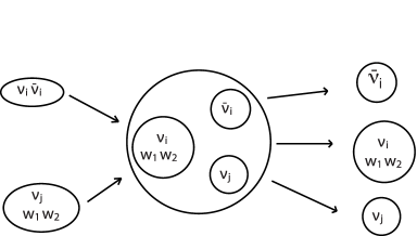
Figure 19.3. $\nu_{i}\neq\nu_{j},\nu_{i}=\nu_{e},\nu_{\mu},\nu_{\tau}.$

19.5. Strong and mixed decays

19.5.1. Strong decays.

Consider the following types of decays:

$$\Delta^{++}\longrightarrow p+\pi^{+}.$$

The complete decay process should be

(19.22) $$\Delta^{++}+\phi_{g}+2\phi_{\gamma}\longrightarrow p+\pi^{+}.$$

It is clear that the final particles are the proton and charged $\pi$ meson $\pi^{+}$. Hence (19.22) is a strong type of decays. Recalling the weakton constituents, (19.22) is rewritten as

(19.23) $$3w^{\ast}w_{1}\bar{w}_{1}(\Delta^{++})+w^{\ast}\bar{w}^{\ast}(\phi_{g})+w_{1}\bar{w}_{1}+w_{2}\bar{w}_{2}(\phi_{\gamma})$$

$$\qquad\qquad\longrightarrow(2w^{\ast}w_{1}\bar{w}_{1})(w^{\ast}w_{1}w_{2})(p)+(w^{\ast}w_{1}\bar{w}_{1})(\bar{w}^{\ast}\bar{w}_{1}\bar{w}_{2})(\pi^{+}).$$

The reaction process in (19.23) consists of two steps:

(19.24) weakton exchanges: $$\phi_{g}+2\phi_{\gamma}\quad\longrightarrow\quad d+\bar{d},$$

(19.25) quark exchanges: $$uuu+d\bar{d}\quad\longrightarrow\quad uud+u\bar{d}.$$

The exchange mechanism of (19.24) was discussed in (19.21), which is a weak interaction, and the quark exchange (19.25) is a strong interaction.

Let us discuss the $D^{0}$ decay, which is considered as the weak interacting type in the classical theory. But in our classification it belongs to strong type of interactions. The $D^{0}$ decay is written as

$$D^{0}\longrightarrow K^{-}+\pi^{+}.$$

The complete formula is

(19.26) $$D^{0}+g+2\gamma\longrightarrow K^{-}+\pi^{+}.$$

The weakton constituents of this decay is given by

(19.27) $$(w^{\ast}w_{2}\bar{w}_{2})(\bar{w}^{\ast}\bar{w}_{1}w_{1})(c\bar{u})+w^{\ast}\bar{w}^{\ast}(g)+2w_{1}\bar{w}_{1}(\gamma)$$

$$\qquad\qquad\longrightarrow(w^{\ast}w_{1}w_{2})(\bar{w}^{\ast}\bar{w}_{1}w_{1})(s\bar{u})+(w^{\ast}w_{1}\bar{w}_{1})(\bar{w}^{\ast}\bar{w}_{1}\bar{w}_{2})(u\bar{d}).$$

This reaction is due to the c-quark decay

$$c+g+2\gamma\to s+u+\bar{d},$$

which is given in the weakton constituent form as

(19.28) $$w^{\ast}w_{2}\bar{w}_{2}(c)+w^{\ast}\bar{w}^{\ast}(g)+2w_{1}\bar{w}_{1}(\gamma)$$

$$\qquad\qquad\longrightarrow w^{\ast}w_{1}w_{2}(s)+w^{\ast}w_{1}\bar{w}_{1}(u)+\bar{w}^{\ast}\bar{w}_{1}\bar{w}_{2}(\bar{d}).$$

The reaction (5.28) consists of two exchange processes:

(19.29) $$w^{\ast}w_{2}\bar{w}_{2}(c)+w_{1}\bar{w}_{1}(\gamma)\to w^{\ast}w_{1}w_{2}(s)+\bar{w}_{1}\bar{w}_{2}(W^{-}),$$

(19.30) $$\bar{w}_{1}\bar{w}_{2}(W^{-})+w_{1}\bar{w}_{1}(\gamma)+w^{\ast}\bar{w}^{\ast}(g)\to w^{\ast}w_{1}\bar{w}_{1}(u)+\bar{w}^{\ast}\bar{w}_{1}\bar{w}_{2}(\bar{d}).$$

It is clear that both exchanges here belong to weak interactions. However, the final particles of the $D^{0}$ decay are $K^{-}$ and $\pi^{+}$, which are separated by the strong hadron repelling force.

19.5.2. Mixed decays

We only consider the $\Lambda$ decay:

(19.31) $$\Lambda\to p+\pi^{-}.$$

The correct form of this decay should be

(19.32) $$\Lambda+g+2\gamma+\phi_{\gamma}\to p+\pi^{-}+\phi_{\gamma}.$$

There are three exchange procedures in (19.32):

(19.33) $$g+\gamma+\phi_{\gamma}\to u+\bar{u},$$

(19.34) $$s+\gamma\to d+\phi_{\gamma}, (uds+\gamma\to udd+\phi_{\gamma})$$

(19.35) $$udd(n)+u\bar{u}\to uud(p)+u\bar{d}(\pi^{-}).$$

The procedure (19.33) was described by (19.20), the quark exchange process (19.35) is clear, and (19.34) is the conversion from $s$ quark to $d$ quark, described by

(19.36) $$w^{\ast}w_{1}w_{2}\uparrow\downarrow\downarrow(s)+w_{1}\bar{w}_{1}\uparrow\uparrow(\gamma)\longrightarrow w^{\ast}w_{1}w_{2}\uparrow\uparrow\downarrow(d)+w_{1}\bar{w}_{1}\downarrow\uparrow(\phi_{\gamma}).$$

Namely, (19.36) is an exchange of two $w_{1}$ with reverse spins.

20. Electron Radiations

20.1. Electron structure

The weakton constituents of an electron are $\nu_{e}w_{1}w_{2}$, which rotate as shown in Figure 18.2. Noting that

electric charge: $$Q^{\nu}_{e}=0, Q_{e}^{w_{1}}=-\frac{1}{3}, Q_{e}^{w_{2}}=-\frac{2}{3},$$

weak charge: $$Q^{\nu}_{w}=1, Q_{w}^{w_{1}}=1, Q_{w}^{w_{2}}=1,$$

we see that the distribution of weaktons $\nu_{e}$, $w_{1}$ and $w_{2}$ in an electron is in an irregular triangle due to the asymptotic forces on the weaktons by the electramagnetic and weak interactions, as shown in Figure 20.1.

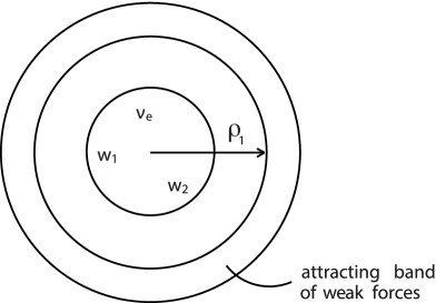
Figure 20.1. Electron structure.

In addition, by the weak force formula (17.24), there is an attracting shell region of weak force:

(20.1) $$\rho_{1}<r<\rho_{2},\qquad\rho_{1}=10^{-16}\text{ cm}$$

with small weak force. Outside this region, the weak force is repelling:

(20.2) $$F_{w}>0\qquad\text{ for }r<\rho_{1}\quad\text{ and }r>\rho_{2}.$$

Since the mediators $\gamma$, $\phi_{\gamma}$, $g$, $\phi_{g}$ and $\phi_{\nu}$ contain two weak charges $2g_{w}$, they are attached to the electron in the attracting shell region (20.1), forming a cloud of mediators. The irregular triangle distribution of the weaktons $\nu_{e}$, $w_{1}$ and $w_{2}$ generate a small moment of force on the mediators in the shell region, and there exist weak forces between them. Therefore the bosons will rotate at a speed lower than the speed of light, and generate a small mass attached to the naked electron $\nu_{e}w_{1}w_{2}$.

20.2. Mechanism of Bremsstrahlung

It is known that an electron emits photons as its velocity changes. This is called bremsstrahlung, and the reasons why bremsstrahlung can occur is unknown in classical theories. We present here a mechanism of this phenomena based on the above mentioned structure of electrons.

In fact, as an electron is in an electromagnetic field, which exerts a Coulomb force on its naked electron $\nu_{e}w_{1}w_{2}$, but not on the attached neutral mediators. Thus, the naked electron changes its velocity, which draws the mediator cloud to move as well, causing a perturbation to moment of force on the mediators. As the attracting weak force in the shell region (20.1) is small, under the perturbation, the centrifugal force makes some mediators in the cloud, such as photons, flying away from the attracting shell region, and further accelerated by the weak repelling force (20.2) to the speed of light, as shown in Figure 20.2.

Figure 20.2. (a) The naked electron is accelerated in an electromagnetic field; (b) the mediators (photons) fly away from the attracting shell region under a perturbation of moment of force.

21. Conclusions of Part 2

The main motivation of this part is that the sub-atomic decays amounts to saying that quarks and charged leptons must possess interior structure. With this motivation, a weakton model of elementary particles is proposed based on 1) sub-atomic particle decays, and 2) formulas for the weak and strong interaction potentials/forces. In this weakton model, the elementary particles consist of six spin-$\frac{1}{2}$ massless particles, which we call weaktons, and their antiparticles. The weakton model leads to 1) composite constituents for quarks, charged leptons and medaitors, 2) a new mass generation mechanism, and 3) a perfect explanation of all sub-atomic decays and reactions.

With this weakton model and the unified field theory [17] and in Part 1 of this article, we now present our explanations and viewpoints to the twelve fundamental questions stated in the Introduction.

Q₁: Our current view on four interactions is that each interaction has its own charge, the mass charge $m$, the electric charge $e$, the weak charge $g_{w}$ and the strong charge $g_{s}$, which are introduced in Section 17.3. Each weakton carries one unit of weak charge, hence the name weakton, and only $w^{\ast}$ carries a unit of strong charge $g_{s}$. A particular interaction can only occur between two particles if they both carry charges of the corresponding interaction.

The dynamic laws for four interactions are the unified field model, which can be easily decoupled to study individual interactions. Our theory shows that each interaction has both attractive and repulsive regions, leading the stability of matter in our universe.

Q₂: With the weakton model, it is clear that leptons do not participate strong interactions, as they do not carry any strong charge–the weakton constituents of charged leptons (18.5) do not include $w^{\ast}$.

Q₃: The weakton model postulates that all matter particles (leptons, quarks) and mediators are made up of massless weaktons. The basic mass generation mechanism is presented in Section 17.2. Namely, for a composite particle, the constituent massless weaktons can decelerate by the weak force, yielding a massive particle, based on the Einstein mass-energy relation. Also, the constituent weaktons are moving in an “asymptotically-free” shell region of weak interactions as indicated by the weak interaction potential/force formulas, so that the bounding and repelling contributions to the mass are mostly canceled out. Hence the mass of a composite particle is due mainly to the dynamic behavior of the constituent weaktons.

Q₄ & Q₅: In Sections 19.1-19.5, the weakton model offers a perfect explanation for all sub-atomic decays and all generation/annihilation precesses of matter-antimatter. In particular, all decays are achieved by 1) exchanging weaktons and consequently exchanging newly formed quarks, producing new composite particles, and 2) separating the new composite particles by weak and/or strong repelling forces. Also, we know now the precise constituents of particles involved in all decays both before and after the reaction.

Q₆: Again, the sub-atomic decays and reactions offer a clear evidence for the existence of interior structure for quarks and leptons, as well as for mediators. The consistency of the weakton model with all reactions and decays, together with conservations of quantum numbers, demonstrates that both quarks and charged leptons are not elementary particles.

Q₇ (Baryon Asymmetry): Conventional thinking was that the Big Bang should have produced equal amounts of matter and antimatter, which will annihilate each other, resulting a sea of photons in the universe, a contradiction to reality. The weakton model offers a complete different view on the formation of matter in our universe. The weakton model says that what the Big Bang produced was a sea of massless elementary weaktons and anti-weaktons, forming all the matter, including mediators such as photon, in the universe. Hence with the weakton model, the baryon asymmetry problem is no longer a right question to ask.

Q₈–Q₁₁: The decoupled unified field model leads to three levels of strong interaction potentials and two levels of weak interaction potentials as recalled in (17.11)–(17.13), (17.19) and (17.20). These formulas give a natural explanation of both the short-range nature and confinements for both strong and weak interactions. The different levels of each interaction demonstrate that in the same spatial region, the interaction can be attracting between weaktons, and be repelling for newly formed hadrons and leptons. This special feature of weak and strong interactions plays a crucial rule for decays.

Q₁₂ (Bremsstrahlung): The weak interaction force formulas show that the attracting shell region near a naked electron can contain a cloud of neutral mediators as photon. As the naked electron changes its velocity due to the presence of an electromagnetic field, which has no effect on the neutral mediator cloud. The change of velocity of electron generates a perturbation to moment of force on the mediators causing some of the mediators flying out from the attracting shell region. This is the mechanism of bremsstrahlung; see Sections 20.1 and 20.2.

References

- [1] H. A. Atwater, Introduction to general relativity, Pergamon Press, Oxford, 1974. International Series of Monographs in Natural Philosophy, Vol. 63.
- [2] E. J. Eichten, K. D. Lane, and M. E. Peskin, New tests for quark and lepton substructure, Phys. Rev. Lett., 50 (1983), pp. 811–814.
- [3] F. Englert and R. Brout, Broken symmetry and the mass of gauge vector mesons, Physical Review Letters, 13 (9) (1964), p. 321 23.
- [4] S. Glashow, Gauge theories of vector particles, doe technical report, (1961).
- [5] D. Griffiths, Introduction to elementary particles, Wiley-Vch, 2008.
- [6] G. Guralnik, C. R. Hagen, and T. W. B. Kibble, Global conservation laws and massless particles, Physical Review Letters, 13 (20) (1964), p. 585 587.
- [7] F. Halzen and A. D. Martin, Quarks and leptons: an introductory course in modern particle physics, John Wiley and Sons, New York, NY, 1984.
- [8] H. Harari, A schematic model of quarks and leptons, Physics Letters B, 86 (1979), pp. 83–86.
- [9] P. W. Higgs, Broken symmetries and the masses of gauge bosons, Physical Review Letters, 13 (1964), p. 508 509.
- [10] M. Kaku, Quantum Field Theory, A Modern Introduction, Oxford University Press, 1993.
- [11] G. Kane, Modern elementary particle physics, vol. 2, Addison-Wesley Reading, 1987.
- [12] E. H. Lieb and R. Seiringer, The Stability of Matter in Quantum Mechanics, Cambridge University Press, 2009.
- [13] T. Ma and S. Wang, Duality theory of strong interaction, Indiana University Institute for Scientific Computing and Applied Mathematics Preprint Series, #1301: http://www.indiana.edu/~iscam/preprint/1301.pdf, (2012).
- [14] , Duality theory of weak interaction, Indiana University Institute for Scientific Computing and Applied Mathematics Preprint Series, #1302: http://www.indiana.edu/~iscam/preprint/1302.pdf, (2012).
- [15] , Gravitational field equations and theory of dark matter and dark energy, Discrete and Continuous Dynamical Systems, Ser. A, in press; see also arXiv:1206.5078v2, (2012).
- [16] , Structure and stability of matter, Indiana University Institute for Scientific Computing and Applied Mathematics Preprint Series, #1303: http://www.indiana.edu/~iscam/preprint/1303.pdf, (2012).
- [17] , Unified field equations coupling four forces and principle of interaction dynamics, arXiv:1210.0448, (2012).
- [18] , Weakton model of elementary particles and decay mechanisms, Indiana University Institute for Scientific Computing and Applied Mathematics Preprint Series, #1304: http://www.indiana.edu/~iscam/preprint/1304.pdf, (May 30, 2013).
- [19] Y. Nambu, Spontaneous symmetry breaking in particle physics: a case of cross fertilization, http://www.nobelprize.org/nobel_prizes/physics/laureates/2008/nambu-slides.pdf, (2008).
- [20] J. C. Pati and A. Salam, Lepton number as the fourth ”color”, Phys. Rev. D, 10 (1974), pp. 275–289.
- [21] C. Quigg, Gauge theories of the strong, weak, and electromagnetic interactions, Benjamin/Cummings Reading, Mass., 1983.
- [22] A. Salam, Elementary particle theory, ed. svaratholm. stockholm, (1968).
- [23] M. A. Shupe, A composite model of leptons and quarks, Physics Letters B, 86 (1979), pp. 87–92.
- [24] S. Weinberg, A model of leptons, Phys. Rev. Lett., 19 (1967), pp. 1264–1266.
- [25] N.-S. Zhang, Particle Physics, vol. I & II, in Chinese, Chinese Academic Press, 1994.