Probing novel TeV physics through precision calculations of scalar and tensor charges of the nucleon

Abstract:

We present an update on the calculation of matrix elements of iso-vector scalar, axial and tensor charges between a neutron and a proton state. These matrix elements are needed to probe novel scalar and tensor interactions in neutron beta-decay that can arise in extensions of the Standard Model at the TeV scale. Our calculations are being done using valence clover fermions on dynamical $N_{f}=2+1+1$ HISQ configurations generated by the MILC Collaboration. We provide preliminary estimates of the dependence of these matrix elements on the light quark masses, lattice spacing, and the time separation between the source and sink of the nucleons. We also find that the renormalization constants calculated using the RI-sMOM scheme are close to unity for the HYP smeared HISQ lattices.

1 Introduction

The observed electroweak symmetry breaking in the Standard Model (SM) points to new physics at the TeV scale, which is currently being explored at the LHC. There are many candidate extensions of the SM, such as supersymmetry and extra dimensions, but, so far, there is no experimental guidance on what new interactions and particles exist at this scale. A theoretical approach (effective field theory) is to postulate new interactions at the TeV scale (without necessarily specifying a model) and analyze the corrections they would give rise to in low-energy (few-GeV) physics. Precision measurements of decays can then be used to bound the allowed parameter space of the posulated interactions. In Ref. [1], we have shown that precision measurements of decays of (ultra)cold neutrons at the $10^{-3}$ level can be used to improve the bounds on new scalar and tensor interactions at the TeV scale provided estimates accurate to 10–20% of the matrix elements of isovector scalar and tensor bilinear quark operators are realized.

In these proceedings, we will summarize the progress we have made in the needed calculations to extract the charges $g_{A}$, $g_{S}$ and $g_{T}$. These charges are defined as

$$g_{A}=Z_{A}\langle p|O_{A}|n\rangle\ ;\ \ \ g_{S}=Z_{S}\langle p|O_{S}|n\rangle\ ;\ \ \ g_{T}=Z_{T}\langle p|O_{T}|n\rangle\ ,$$

where $Z_{\Gamma}$ are the corresponding renormalization constants, which we calculate nonperturbatively in the RI-sMOM scheme [2, 3]. This report is a follow up to Ref. [1], and we will use the notation established there. The calculations are being done using the 2+1+1 flavor HISQ lattices being generated by the MILC Collaboration [4]. Clover fermions on HYP smeared HISQ lattices are being used for constructing the correlation functions. Three values of the lattice spacing are being analyzed, $a=0.12$, $0.09$ and $0.06$ fm, to perform the continuum extrapolation, and at each lattice spacing we analyze two values of the light quark masses corresponding to $M_{\pi}\approx 310$ and $220$ MeV. We will address the following sources of statistical and systematic errors in the extraction of matrix elements and, from them, the charges.

• The signal and the statistical errors in the two- and three-point correlation functions.

• The dependence of $g_{A,S,T}$ on the light-quark (pion) masses and lattice spacing to estimate uncertainty due to chiral and continuum extrapolations.

• The effect of contamination by excited states.

• Estimates of the renormalization constants calculated in the RI-sMOM scheme.

A similar analysis has been reported in Ref. [5] at this conference.

2 Statistics

The MILC Collaboration has produced ensembles of roughly 5500 trajectories of 2+1+1 flavor HISQ lattices at each of the six values of quark masses and lattice spacings we are analyzing as described in Table 1. Five hundred trajectories are discarded for thermalization. Configurations are then analyzed separated by five trajectories. On each configuration, four smeared sources, displaced both in time and space directions to reduce correlations, are used. Furthermore, two sets of these four source points, again maximally separated in space and time directions, are used on each alternate configuration to reduce correlations. The roughly 500 configurations with each of these two sets of sources are also analyzed separately. We verify that the two sets give compatible results and the errors are roughly $\sqrt{2}$ larger compared to the full set. Our main conclusion is that with 1000 or more configurations one gets a statistically significant signal needed for obtaining the design accuracy of 10–20% in both the 2-point and 3-point functions for all cases. Extraction of $g_{S}$ is the nosiest and drives the overall sensitivity as discussed below.

$a$ (fm)	$m_{l}/m_{s}$	$M_{\pi}$ (MeV)	$L^{3}\times T$	$M_{\pi}L$	Configs (Z)	Configs (ME)	$\Delta t$
0.12	0.2	305	$24^{3}\times 64$	4.54	50	1013/1013	8,9,10,11,12
0.12	0.1	217	$32^{3}\times 64$	4.29	50	958/958	8,10,12
0.09	0.2	313	$32^{3}\times 96$	4.5		391/1000	12,14
0.09	0.1	220	$48^{3}\times 96$	4.73		443/1000	12,14
0.06	0.2	320	$48^{3}\times 144$	4.53		330/1000	16,20
0.06	0.1	229	$64^{3}\times 144$	4.28		0/1000

Table 1: Lattice parameters of the six ensembles of 2+1+1 flavor HISQ lattices analyzed. We give a status report (as of November 2012) on the number of analyzed and total configurations used in calculations of ME and for the calculation of renormalization constants (Z). The last column gives in lattice units the time seperations $\Delta t$ between source and sink investigated to understand the excited-state contamination.

3 Excited-State Contamination

The desired matrix elements need to be calculated between ground state nucleons. The operators used to create and annihilate the states, however, couple to the nucleon and all its excited states. There are two possible ways to reduce contribution from excited states: by reducing the overlap of the interpolating operator with the excited states and by increasing the time separation $\Delta t$ between the source and sink to exponentially suppress excited-state contamination. Statistics limit the upper value of $\Delta t$ that can be explored. We use smeared sources and sinks to reduce overlap and investigate up to five time separations.

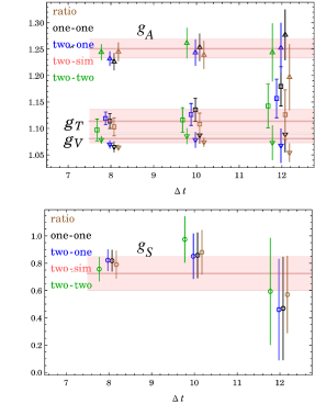
Figure 1: Estimates of the unrenormalized charges $g_{A}$, $g_{V}$, $g_{S}$ and $g_{T}$ from the five different fits for the $a=0.12$ fm lattices with $M_{\pi}$ = 310 MeV (left) and 220 MeV (right). The bands correspond to the 2-2 simultaneous fit described in the text and are used as our best estimates. The other four estimates are consistent with this estimate. $\Delta t$ is the separation in time between the source and the sink in lattice units.

Assuming that all excited-state contamination can be represented by a single excited state with amplitude $A_{1}$ and mass $M_{1}$, we can write the 3-point function with source at $t=0$, operator insertion at $t=t$ and sink at $t=\Delta t$ as

$${\cal C}_{\Gamma} = |A_{0}|^{2}\langle 0|O_{\Gamma}|0\rangle e^{-M_{0}{\Delta t}}+|A_{1}|^{2}\langle 1|O_{\Gamma}|1\rangle e^{-M_{1}{\Delta t}}+$$ (1)

$$A_{0}A_{1}^{*}\langle 0|O_{\Gamma}|1\rangle e^{-M_{0}t}e^{-M_{1}({\Delta t}-t)}+A_{0}^{*}A_{1}\langle 1|O_{\Gamma}|0\rangle e^{-M_{1}t}e^{-M_{0}({\Delta t}-t)}$$

where $\Gamma$ represents one of the sixteen Clifford elements defining the bilinears. To extract $\langle 0|O_{\Gamma}|0\rangle$ from the 2- and 3-point functions we examine five different fits. All errors are estimated with the full analysis done within a single-elimination jackknife method.

• 1-1 method assumes a single state dominates the 2-pt and 3-pt functions. $A_{0}$ and $M_{0}$ are extracted from a fit to the 2-pt function and $\langle 0|O_{\Gamma}|0\rangle$ are estimated from the 3-pt functions keeping only the first term in Eq. (1).

• Ratio method also assumes a single state dominates the 3-pt function. $\langle 0|O_{\Gamma}|0\rangle$ are estimated from the ratio of 3-pt to 2-pt functions. While some of the systematics cancel in the ratio, this fit relies on there being a good signal in the 2-pt function at separation $\Delta t$.

• 2-1 method: $A_{0}$, $A_{1}$, $M_{0}$ and $M_{1}$ are extracted from a fit to the 2-pt function. Of these, only $A_{0}$ and $M_{0}$ are used to estimate $\langle 0|O_{\Gamma}|0\rangle$ by fitting to the first term in Eq. (1).

• 2-2 method extracts $A_{0}$, $A_{1}$, $M_{0}$ and $M_{1}$ from a fit to the 2-pt function. These amplitudes and masses are used in a 2-parameter fit to the 3-pt function to estimate $\langle 0|O_{\Gamma}|0\rangle$ and $\langle 1|O_{\Gamma}|0\rangle$. We assume $\langle 0|O_{\Gamma}|1\rangle$ and $\langle 1|O_{\Gamma}|0\rangle$ are equal and we analyze only the real part of the 3-point function. We also neglect $\langle 1|O_{\Gamma}|1\rangle$.

• 2-2 simultaneous fit to all $\Delta t$ is the same as the 2-2 method for extracting $A_{0}$, $A_{1}$, $M_{0}$ and $M_{1}$. The fit to the 3-point function uses data for all investigated values of $\Delta t$ simultaneously.

Our current understanding of excited-state contamination is based on the analysis of the full set of 1013 configurations for the $a=0.12$ fm $M_{\pi}=310$ MeV ensemble using $\Delta t=8,\ 9,\ 10,\ 11,\ 12$ and 958 configurations for the $a=0.12$ fm $M_{\pi}=310$ MeV ensemble using $\Delta t=8,\ 10,\ 12$. These data are shown in Fig. 1. The vector charge $g_{V}$ is shown only as a check.

We find that the ratio method exhibits plateaus for $g_{A}$, $g_{V}$ and $g_{T}$, so it is not surprising that the first four methods give consistent estimates. The estimates from the 2-2 simultaneous fit method are shown by the horizontal bands which we take as our best estimates. Our observations, based on these two ensembles of roughly 1000 configurations and smeared sources used by us in calculating quark propagators, are:

• On the $0.12$ fm lattices, the statistical errors increase by about $40$% with each unit increase in $\Delta t$. We find a similar increase for the $a=0.09$ and $0.06$ fm lattices once the unit increase in $\Delta t$ is scaled by the factors $1.33$ and $2$ to keep distances constant in physical units.

• There is a small trend showing an increase (within $1\sigma$) in $g_{A}$ and $g_{T}$ with $\Delta t$.

• For $t>12$, even the signal in the 2-point nucleon correlator becomes noisy. Based on the trends seen in the $M_{\pi}=310$ MeV ensemble, we considered it sufficient to investigate the $M_{\pi}=220$ MeV ensemble using $\Delta t=8,\ 10,\ 12$.

• The 2-2 simultaneous fit estimates of the central values and errors are consistent with data from other fits for all values of $\Delta t$.

• The errors increase by about 20% on lowering the light ($u$ and $d$) quark masses by a factor of two $i.e.$ from $M_{\pi}=310$ to $220$ MeV ensembles.

• The signal in $g_{S}$ is the noisiest. On the $M_{\pi}=220$ MeV ensembles, the error estimate is $\approx 20\%$, reasonably close to the desired accuracy.

• The statistical signal improves significantly as $a$ is reduced. This is presumably due to the larger lattice volumes and smoother gauge configurations. Preliminary results show that on the $a=0.09$ and $0.06$ fm ensembles we will be able to extract even $g_{S}$ within $10\%$ accuracy.

Our conclusion, based on the $a=0.12$ fm lattices, is that the central values from the 2-2 simultaneous fit agree with those from the other fits for separation $\Delta t=10$ which corresponds to $\approx 1.2$ fm. We, therefore, consider the $\Delta t=10$ ($i.e.$ in physical units this $\Delta t=1.2$ fm) data the best compromise between reducing excited-state contamination and having a good statistical signal. The choice of $\Delta t$ values investigated on the $a=0.09$ and $0.06$ fm ensembles is based on these conclusions.

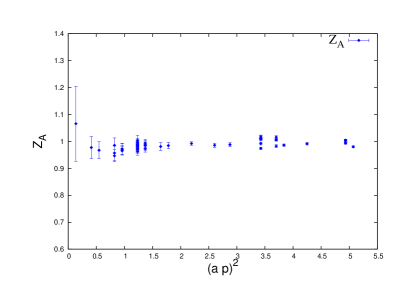
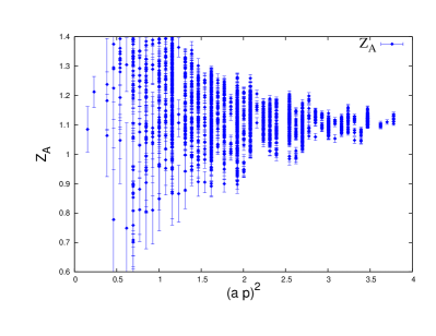
$Z_{A}$ ($M_{\pi}=310$ MeV ensemble)	$Z_{A}$ ($M_{\pi}=220$ MeV ensemble)
$Z_{S}$ ($M_{\pi}=310$ MeV ensemble)	$Z_{S}$ ($M_{\pi}=220$ MeV ensemble)
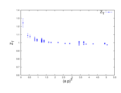
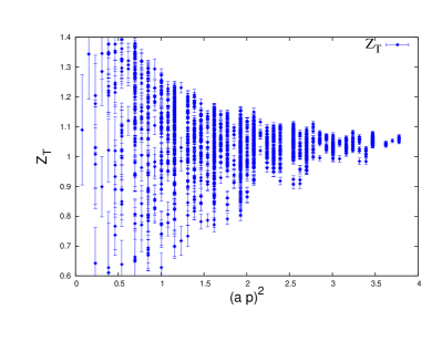
$Z_{T}$ ($M_{\pi}=310$ MeV ensemble)	$Z_{T}$ ($M_{\pi}=220$ MeV ensemble)

Figure 2: The data for the renormalization constants $Z_{A}$, $Z_{S}$ and $Z_{T}$ for the $a=0.12$ fm lattices as a function of the momenta $p_{i}^{2}=p_{f}^{2}=(p_{i}-p_{f})^{2}$. Note that $p=1.6$ GeV for $pa=1$. The analysis is done using point source Wilson-Clover action propagators calculated on HYP smeared HISQ lattices. For these ensambles, we find that estimates of all three $Z_{\Gamma}$ are within $10\%$ of unity. The dependence on the light quark mass, $i.e.$, the $\sim$ 10% increase on going from the $M_{\pi}=310$ to $220$ MeV ensembles, is being studied.

4 Dependence on Quark Mass and Lattice Spacing

The data show a small increase in the values of the bare charges $g_{A}$, $g_{S}$ and $g_{T}$ on going from $M_{\pi}=310$ to $220$ MeV ensemble for $a=0.12$fm. The change is, however, within $1\sigma$. The data for the $a=0.09$ and $0.06$ fm lattices are too preliminary to draw conclusions on the dependence on either the quark mass or on the lattice spacing. Since the statistical signal improves as $a\to 0$, we anticipate that our final results will shed light on possible dependence on the quark mass and the lattice spacing.

5 Renormalization Constants $Z_{\Gamma}$

The renormalization constants $Z_{\Gamma}$ are calculated in the RI-sMOM scheme using point source propagators evaluated on Landau gauge fixed lattices. The data for $a=0.12$ fm ensembles are shown in Fig. 2. In this scheme only momenta satisfying $p_{i}^{2}$ = $p_{f}^{2}$ = $(p_{i}-p_{f})^{2}$ are examined (the $M_{\pi}=310$ MeV lattices have much fewer momenta satisfying this condition due to the smaller lattice volume), and the data have been averaged over points equivalent under cubic symmetry. We find that for the HYP smearing used in the calculation, all the renormalization constants are already within $10\%$ of unity at $a=0.12$ fm. We are currently investigating $O(p^{4})$ contributions in these estimates to reduce these discretization effects.

6 Conclusions

We show that the excited-state contamination is smaller than statistical errors for source-sink separation greater than $1.2$ fm. The renomalization constants in the RI-sMOM scheme are within 10% of unity already on the coarsest lattices at $a=0.12$ fm. We therefore, conclude that $O(1000)$ lattices will be sufficient to get estimates with 10–15% precision for both $g_{S}$ and $g_{T}$ at all three values of the lattice spacing. We anticipate completing the analysis on the $a=0.09$ and $0.06$ fm lattices over the next year. These data are needed to confirm the small observed dependence on the quark mass and lattice spacing, and before conclusions on the chiral and continuum extrapolations can be drawn.

References

- [1] T. Bhattacharya, , Probing Novel Scalar and Tensor Interactions from (Ultra)Cold Neutrons to the LHC, Phys.Rev. D85 (2012) 054512.
- [2] G. Martinelli, , Nucl. Phys. B 445, (1995) 81. [arXiv:hep-lat/9411010].
- [3] C. Sturm, , Phys. Rev. D 80, (2009) 014501. [arXiv:0901.2599 [hep-ph]].
- [4] MILC Collaboration, http://physics.indiana.edu/~sg/milc.html.
- [5] J. Green, , [arXiv:1211.0253 [hep-ph]].
- [6] R. Edwards and B. Joo, The Chroma Software System for Lattice QCD, Nucl. Phys. Proc. Suppl. 140 (2005) 832