Fast Rise of “Neptune-Size” Planets () from to days
– Statistics of Kepler Planet Candidates Up to
Abstract
We infer the period () and size () distribution of Kepler transiting planet candidates with and hosted by solar-type stars. The planet detection efficiency is computed by using measured noise and the observed timespans of the light curves for Kepler target stars. We focus on deriving the shape of planet period and radius distribution functions. We find that for orbital period , the planet frequency d/dP for “Neptune-size” planets () increases with period as . In contrast, d/dP for “super-Earth-size” () as well as “Earth-size” () planets are consistent with a nearly flat distribution as a function of period ( and , respectively), and the normalizations are remarkably similar (within a factor of at ). Planet size distribution evolves with period, and generally the relative fractions for big planets () increase with period. The shape of the distribution function is not sensitive to changes in selection criteria of the sample. The implied nearly flat or rising planet frequency at long period appears to be in tension with the sharp decline at in planet frequency for low mass planets (planet mass ) recently suggested by HARPS survey. Within , the cumulative frequencies for Earth-size and super-Earth-size planets are remarkably similar ( and ), while Neptune-size and Jupiter-size planets are , and , respectively. A major potential uncertainty arises from the unphysical impact parameter distribution of the candidates.
1. Introduction
The Kepler mission provides an unprecedented opportunity to study the size and period distribution of extrasolar planets down to Earth radii within yr-long orbits by making high-precision (), high-cadence () and nearly-continuous monitoring of stars over years. Based on the transiting planet candidates discovered from the first 4 months of Kepler data (Borucki et al. 2011, hereafter B11), Howard et al. (2012) (hereafter H12) made a statistical inference of the frequency for planets with radii . H12 found that planet frequency increases for decreasing radii, and that it drops sharply for planets with very close-in orbits (). They claimed that the Kepler planet frequencies are consistent with those found by radial-velocity (RV) surveys (Mayor et al., 2009; Howard et al., 2010). Several other studies also use the B11 sample to study planet distribution. Gould & Eastman (2011) found that there is a break in the radius distribution of B11 candidates at . By extrapolating the detection efficiency deduced by H12 and applying a maximum-likelihood approach, Youdin (2011) fitted the distribution of B11 candidates down to and found a relative deficiency of planets at . Catanzarite & Shao (2011) and Traub (2012) attempted to extrapolate the planet frequency obtained from B11 candidates to estimate the fraction of Sun-like stars that host habitable Earth-like planets.
The latest release of Kepler based on 16 months (quarters Q1-Q6) of data (Batalha et al. 2012, hereafter B12) has increased the number of known planet candidates by a factor of (from to ). As expected, there is a large gain in planet candidates at long periods as well as small radii compared to B11. According to B12, there is also a considerable unexpected gain relative to B11 for short-period planets merely due to the effects of increasing the length of the observing windows, and the implied lower-than-expected efficiency of the planet search pipeline employed by B11 may affect the above-mentioned statistical results. One important improvement in B12 is that for the first time the Kepler team stitched different quarters together in the transit search, which particularly increased the robustness of the search for long-period planets. In fact, two independent automatic planet searches on Q1-Q6 data by Huang et al. (2012) and Ofir & Dreizler (2012) as well as crowd-sourced human identifications by Planet Hunters (Schwamb et al., 2012) only identified a total of more new planet candidates than those found by B12, suggesting that the B12 searches are likely highly efficient.
We derive planet frequency as a function of period and planet radius using Kepler planet candidates discovered by B12 as well as those found by other groups. Like the majority of the works on Kepler statistics to date, we do not distinguish planet candidates from planets, i.e., we assume a low false positive rate (see § 5 for further discussion). The transit planet detection efficiency is calculated for each Kepler star using the measured photometric noise of its light curve and the observed timespan (excluding gaps and missing quarters). In addition, the geometric bias for circular orbits is taken into account. We focus on determining the relative frequency for planets with various radii as a function of period for Sun-like hosts. We find that the distribution of reported impact parameters is unphysical, potentially posing a major uncertainty in the overall normalization of the planet distribution function. We do not distinguish planets in the single or multiple transit systems to derive the planet multiplicity function (Tremaine & Dong, 2012) and we also ignore any possible bias in the detection of single and multiple systems. The Kepler planet frequency derived below extends down to with period up to . This can be compared with the planet frequency inferred from RV searches by 8-yr HARPS survey, which is sensitive to long-period () super-Earth and Neptunes with masses (Mayor et al., 2011).
2. Issues with selecting the Kepler star and planet sample
2.1. The Kepler Input Catalog
Planet frequency is usually defined with respect to an ensemble of host stars that share similar physical properties. Stellar type, metallicity, age and population may have impacts on the frequency of planets. The Kepler target stars were selected based on multi-band photometry (documented in the Kepler Input Catalog, KIC), and the selection was focused on finding solar-type stars to search for Earth analogues.
The KIC photometry is most sensitive to the effective temperature , which is less reliable for constraining surface gravity (particularly unreliable for cool stars) and has little sensitivity to metallicity. We do not attempt to study the planet frequency as a function of metallicity, which would require comprehensive spectroscopic follow-up. The relatively large uncertainty in may have a serious impact on the study of frequency. Unreliable estimates may introduce ambiguity between dwarfs and sub-giants/giants with the same . Furthermore, errors in dominate the uncertainties in the stellar radius measurement, which translates into uncertainty in the planet radius since only planet-to-star radius ratios are measured from transit light curves.
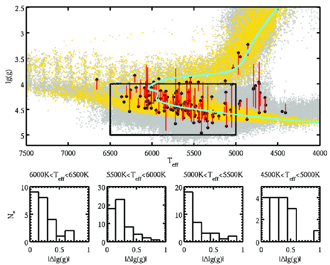
To study the uncertainty in , we use the high-precision stellar parameters derived from high-resolution spectroscopic follow-up of more than a hundred Kepler planet host stars by Buchhave et al. (2012). In the upper panel of Fig.1, the KIC and are plotted as black solid dots, and the values from 104 spectroscopic measurements are plotted at the end of the red lines connected to the KIC values. The majority of the stars in the KIC have between and , and we divide these stars into four equal bins in temperature. For each bin, the average difference between the two sets of measurements is , with no strong systematic preference in sign. The average dispersion is about dex, except for the bin with , which has a dispersion of dex. In the lower panel, the histogram of is shown; for the bin with , of the stars have dex, while stars have for the three other bins. It seems that the problem with uncertainty is most severe for stars with , and we choose not to include them in our stellar sample for this study. The averaged dispersion in for the chosen stellar sample is therefore dex, which translates into dex dispersion in the planet radius estimate.
B12 noted that a considerable fraction of KIC stellar parameters were not consistent with known stellar physics. They matched the KIC , and [Fe/H] with Yonsei-Yale isochrones (Demarque et al., 2004) by minimizing , where is the difference in the KIC and Yonsei-Yale parameters. They reported the stellar parameters (and the derived planet parameters) using the “corrected” values from Yonsei-Yale. We note that the “corrected” stellar parameters do not match the spectroscopic measurements from Buchhave et al. (2012) better than those from the KIC. Nevertheless, they are at least self-consistent for each star according to the known laws of stellar physics (e.g., the parameters match the theoretical mass-radius relation). We follow the procedure by B12 and adopt “corrected” parameters throughout this paper. In Fig.1, the “corrected” and are plotted as yellow dots and the KIC values are shown as gray dots (the Yonsei-Yale isochrone for with solar metallicity is shown in cyan). It is interesting to note that many stars at have KIC values inconsistent with any reasonable isochrones.
Our stellar sample consists of Kepler stars with (approximately corresponding to K2-F5 dwarfs) and . These limits are shown as a black box in Fig.1. We also exclude stars with Kepler magnitude , which consist of a negligible fraction of Kepler stars and have little sensitivity to planets. The sample includes a total number of stars of .
2.2. Impact Parameter Distribution
Only the planets whose orbits are oriented within a limited range of inclination angles are observed to transit their host stars. One basic assumption required to make statistical inference from an ensemble of transiting planets is that the orbital inclinations of planets should be distributed randomly with respect to the observer. Following this assumption, the impact parameters , which are the minimum planet-star projection separations normalized by the radii of the stars during the transits, are distributed uniformly for the observed transits. Then from the observed transits, one may correct for the selection effects due to such geometric conditions (“geometric bias”) to take the number of non-transiting planets into account. For circular orbits, the geometric bias is for transits with .
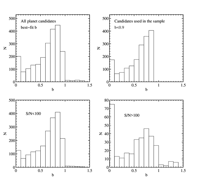
The histogram of best-fit values for Kepler planets reported by B12 is plotted in the upper left panel of Figure 2 as well as the posterior probability distribution considering Gaussian errors in the upper right panel (in the latter case, the unphysical values for due to the Gaussian distribution are shown). The distribution is far from being uniform, and it is highly skewed toward large values (). This unphysical distribution cannot be explained by selection effects due to observation thresholds (transits with low are easier to detect than those with as the former generally have higher S/N). Note that for candidates with high S/N , the distribution is less skewed toward but with a peak at 0 (see the bottom right panel of Fig.2). This is understandable as at low impact parameter, the transit profile is hard to distinguish from those at and the fitting algorithm may set as the best fit.
One possible source of the unphysical distribution of skewing toward may be artifacts or biases introduced by the fitting procedures employed by the Kepler team. One possibility is failure to account for the integration time of the exposure time in the modeling (Kipping 2010, J. Lloyd, B. Gaudi, private communications). The other possible source may be that some of the high- planets are false positives. Note that B12 also includes a small number of grazing transits with significantly larger than 1, and these candidates are unlikely to be of planetary origin. We exclude candidates with impact parameter larger than from our analysis.
Resolving this discrepancy is beyond the scope of this work. In the following analysis, we test whether the planet samples with and result in different distribution functions. Obviously, given the skewed distribution, the normalization of planet frequency has considerable difference between the two samples. We focus on understanding whether the shape of the distribution function is affected by the upper threshold of the impact parameter .
3. Planet Detection Efficiency of Kepler from Detection Thresholds
Besides the geometric selection effect discussed above, the other main selection effect is survey selection, which denotes an incompleteness due to the detection thresholds of the survey. A transit candidate is considered to be detected if (1) the number of transit occurrence exceeds a threshold and (2) the total S/N of the transit signals is greater than the threshold . We discuss both detection thresholds in detail in the following sub-sections.
To characterize the survey selection effects, we introduce the planet detection efficiency , which is the fraction of stars in the stellar sample for which a planet with period and radius can be detected (i.e., the above two thresholds are satisfied). For each star in a sample with a total of stars, the noise and time window during which it is observed, , are known. For a hypothetical planet with and orbiting this star , we calculate and for uniformly distributed phases for the planet transits within time window . Then among the simulations, we count how many of them have both the and criteria satisfied to obtain the fraction of phases where the transits satisfy the detection criteria. Finally, we obtain the detection efficiency for the planet in the sample by summing for all the stars, to be .
The intrinsic planet frequency is defined as,
| (1) |
where is the intrinsic number of planets around host stars. With both detection efficiency and geometric bias known, the intrinsic planet frequency can be derived using the relation,
| (2) |
where is the number of planets that pass the detection thresholds.
In the following two subsection, we will describe how we calculate the two survey selection criteria: (1) , and (2) the S/N threshold
3.1. Threshold
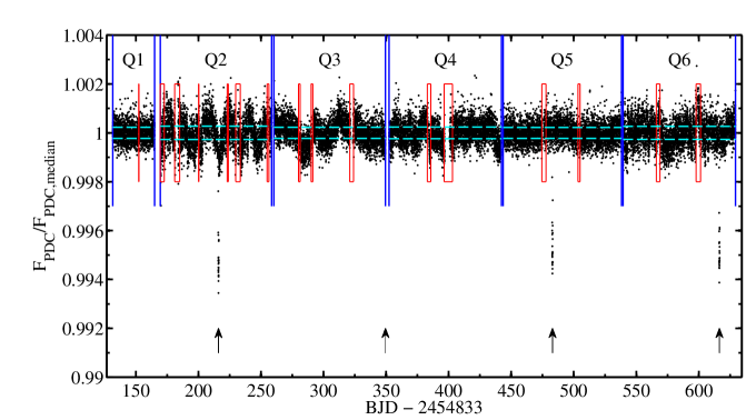
We include the effects of the transit window function, which is important for statistics of long-period planets (Gaudi, 2000). Out of 122328 stars we have selected, have data over all six quarters, and miss and quarters, respectively. Over all 6 quarters, the gaps between quarters and the artifacts amount to a total of , which is of the duration from the start of Q1 to the end of Q6 (see Figure 3. for an example that demonstrates the effect of gaps and Table 1 for a list of the gaps). B12 used the Transiting Planet Search (TPS) module (Tenenbaum et al., 2012) as the primary algorithm to search for periodic square pulses within Q1-Q6 and then sought confirmations in Q7-Q8. Strictly speaking, the TPS module finds transit with at least three occurrences (Tenenbaum et al., 2012), but B12 include planet candidates with fewer transits occurring in their sample. Moreover, the independent searches by Huang et al. (2012) and Ofir & Dreizler (2012) over Q1-Q6 that include transits with less than 3 occurrences only yield more candidates with no obvious preference for long-period ones. For a detection, we adopt a transit occurrence criterion that at least 2 transit occurrences in Q1-Q6 so that it is periodic in this window and 3 transit occurrences in Q1-Q8 so that the detection is secure. We also vary this criterion to demand 3 transit occurrences in Q1-Q6 to check whether we obtain consistent planet statistics in § 5.
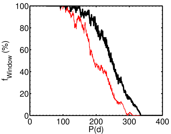
In order to evaluate the effect of window functions, for each trial period, we make 100 simulations with the center of the transits occurring at different times, which are evenly distributed within the period. Then we record the number of transit occurrences for each quarter in each simulation. In Fig.4, we show , the fraction of simulated transits that satisfy the transit occurence criterion as a function of period. The black line represents a star that has been observed over all 8 quarters. starts to decrease from at to at then to at above . We also show an example that has one quarter (Q5) is missing in red line, for which is typically smaller at long periods and no transit satifies the occurrence criterion at . This emphasizes the importance of considering various transit phases for deriving the frequency of planets with long period beyond 100 days.
3.2. S/N Threshold with Box-like Profile
The statistics of the Kepler planet frequency presented in this work are completed by 1) using a simple box-like transit profile for both real and hypothetical planets, and 2) modeling the planet detection threshold with a lower limit in transit signal-to-noise ratio . This is the same assumption made by H12 and B11. The simple box-like transit profile is characterized only by the depth of the transit and the transit duration with the photometric error for . For each star, we have calculated in each individual quarter separately by interpolating the published CDPP values (by the Kepler team) at 3, 6, 12 intervals to the desired transit duration time (for a description of CDPP see Christiansen et al. 2012; the CDPP tables can be downloaded from the official Kepler MAST site). The total S/N from observing box-like transits is,
| (3) |
The box-like transit profile applies in the limit where the planet-to-star radius ratio is small (), there is a zero impact parameter (), and a uniform host star surface brightness profile (no limb-darkening). In this limit, , and for circular orbit. The s for the candidates are calculated using the measured transit durations. Both real and hypothetical planets are considered to be detected when .
In this limit, the dependency of S/N on the impact parameter is ignored. In the experiments we carry out below where we vary the upper threshold for the selection of the planet sample, we simply modify the geometric bias to be . In Dong & Zhu, in prep , we introduce a full framework that takes the effects of limb-darkening and ingress/egress into account. In that case, also introduces changes in the detection efficiency since the S/N detection threshold depends on . Similar to Gould et al. (2006), we find that adding limb-darkening and ingress/egress makes little difference in the inferred distribution.
4. Results
4.1. Kepler Planet Frequency
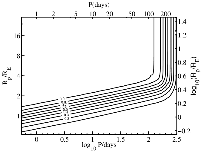
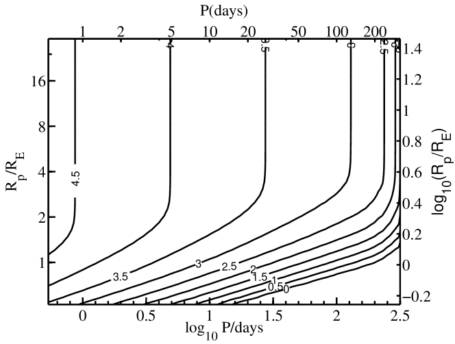
We first carry out the detection efficiency calculations described above for a dense grid of with from to and from to . The grids are divided uniformly in log space for both and . In the main calculation, we choose 111Note that the S/N values we calculate above using CDPP are very close to the Multiple Event Statistics (MES) values reported by B12, which are the quantities used by the main Kepler transit search algorithm TPS which resembles the transit S/N for a periodic square-pulse search. MES must be greater than in the search conducted by Kepler . We adopt a higher threshold , which corresponds to the turnover of the right-hand panel of Fig. 7 of Tenenbaum et al. (2012). The S/N of the transit fit reported by B12 does not have the cut of (with minimum of ) and is on average factor of higher than MES with large variance in ratio between the two quantities. Throughout the paper, we use the S/N values calculated using CDPP to closely mimic the transit detection processes employed by TPS. , and and . All the thresholds are varied in § 5 to make consistency checks. The resulting detection efficiency , and , which represents the planet sensitivity considering both detection efficiency and geometric bias, are shown in the left and right panels of Fig. 5, respectively. Beyond , ’s sensitivity to detect planets drops abruptly.
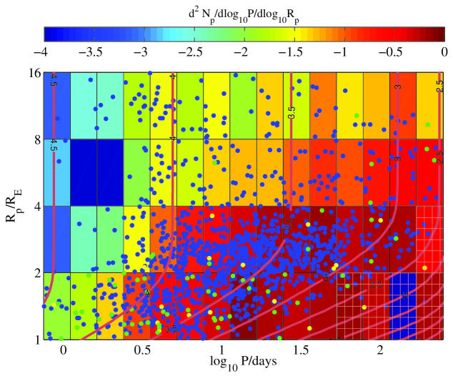
Then, we divide the and plane into bins which are uniformly distributed in , with from to and from to (see Figure 6). In each bin, we take the detection efficiency as well as geometric bias into account and calculate as defined in Equation (2) and its uncertainty assuming a Poisson distribution. In each bin, is assumed to be distributed uniformly in and . For a bin in which there is no planet detected, we compute an upper limit at confidence level. There are 2486 planet candidates in total including B12, Huang et al. (2012), and Ofir & Dreizler (2012), our stellar parameter cuts limit the number of planets to 1801, and 1347 of these survive our detection threshold cut. We examine the effects of adding candidates from Huang et al. (2012) and Ofir & Dreizler (2012) and find that excluding these candidates has negligible impact on the derived planet distributions. The bins in the lower right corners have the least secure statistics due to low sensitivity in detecting planets and relatively large gradients in the sensitivity. The sensitivity is plotted in red lines in Figure 6.
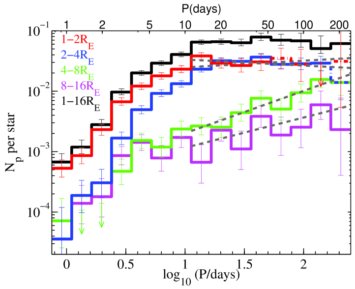
The intrinsic number of planets ( per star) within each period and planet radius bin is shown in Fig. 7. The planet radius bins are (“Jupiter-size”), (“Neptune-size”), (“Super-Earth-size”) and (“Earth-size”). The bin size in (0.3 dex) is chosen to be larger than the averaged dispersion in (dex) due to the uncertainty in KIC estimates. The above-mentioned bins with the least secure statistics are plotted with dash-dotted lines. These include the four longest period bins for Earth-size planets () and the longest period bin for Super-Earth-size planets ().
We confirm the the sharp drop below in planet frequency identified by Howard et al. (2012). Beyond , the most striking feature is that the frequency of Neptune-size planets rises sharply while the smaller planets with from 1-4 have frequency consistent with being flat in . Quantitatively, the frequency of Neptune-size planets increases by a factor of from to . In contrast, the frequencies of Earth-size and super-Earth-size planets are consistent with flat distributions in within 1-2 beyond . The frequency of Jupiter-size planets increases more slowly compared to the rise of the Neptune-size planets. These trends survive by varying several observational cuts (discussed in § 5.1) so they appear to be robust.
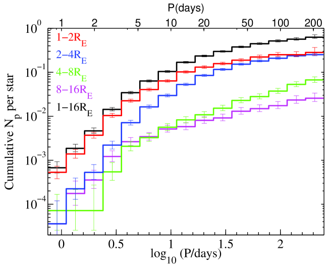
Next we show the cumulative planet frequency for planets with different sizes in Figure 8. Within , Earth-size and Super-Earth-size planets have almost the same cumulative frequency , which is 4 times larger than the Neptune-size planet frequency (), or 10 times larger than the Jupiter-size planet frequency (). The total frequency for all the planets from 1-16 within 250 is 60. However, the absolute normalization is likely not robust as it can vary by a factor as large as depending on various cuts (in particular the impact parameter cut) as discussed in § 5.1 below.
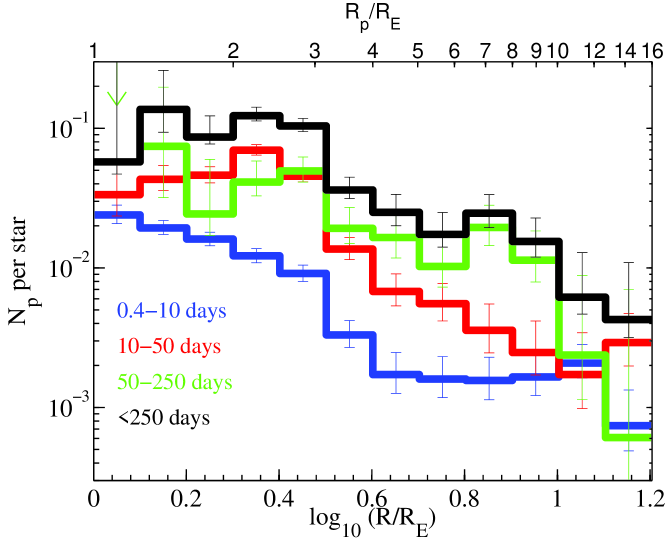
We then show the planet frequency as a function of planet size within three period bins (0.4-10, 10-50, 50-250 ) in Fig.9. There appear to be clear evolution of planet size distribution as a function of period. At all periods, the dominating population in number is the planets with small radii (). There are clear breaks in the distribution function at and . At the shortest period (), below , the planet frequency in increases slowly toward small radii. After a relatively steep drop in frequency at , larger planets are consistent with a flat distribution up to . At longer periods (), below , the distribution is consistent with being flat in (or even consistent with slightly decreasing toward small radii for the bin). We caution that planet statistics presented here are the least secure for at . Within , planet frequency in for planets larger than clearly decreases for increasing radius up to . In the bin with longest periods (), for planets with , the frequency distribution is nearly flat in up to then it drops sharply at . Overall, at longer period, the relative frequency for big planets () compared to small planets () becomes higher.
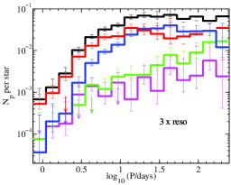
The method presented in this section has the advantage of making no assumption on the functional form of planet distribution, but the data are binned, which has the implicit assumption that planet are distributed uniformly within the bins. Thus, the results may depend on the bin size. We have tested the effects of bin sizes by using bins that are factor of 3 smaller, and the resulting trends in frequency are consistent with those presented above.
4.2. The maximum likelihood method
Motivated by the linear trends seen in the log-log plots in the period distribution for discussed in the previous section, we model these trends with power-law dependencies in period using the maximum likelihood method. This approach has the advantage of requiring no binning.
We follow Tabachnik & Tremaine (2002) and Youdin (2011) to calculate the log likelihood function as
| (4) |
where the sum is taken over all the planet candidates. and are the detection efficiency and the geometric bias as defined above. The intrinsic planet frequency is defined in Eq 1 and the assumed analytical form is
| (5) |
where is also the slope of the intrinsic frequency in the log-log plot. is the expected number of planets with the assumed
| (6) |
We numerically solve the maximum log likelihood for planets in each radius bin (1-2, 2-4, 4-8, 8-16 ). The resulting and are given in table 2. Multiplying with the bin size as in §4.1, we derive the planet frequency, which is over plotted in the left panel of Figure 7 as the gray dashed lines. Our maximum likelihood fits are consistent with the trends in distribution functions described in §4.1, confirming our claims that planets at 1-4 have a nearly flat distribution in beyond 10 days, while planets at 4-8 display a fast increasing distribution in for increasing period .
We assume power-law distributions with respect to planet period for planets in four different radii bins. Figure 9 suggests that the planet radius distribution function is more complicated than simple power-law or broken power-law distribution. We therefore do not attempt to fit analytical functions to the radii distribution with maximum likelihood method. Figure 9 itself is more instructive than such a multi-parameter representation.
5. Discussion
5.1. Varying Sample Selection Cuts
We vary several sample selection cuts to test the robustness of the derived planet frequency.
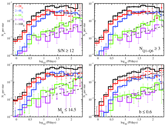
First we vary the detection thresholds: , and the S/N threshold. A S/N threshold=12 (8 is used for the main results) is applied, and the results are shown in the upper left panel of Fig. 10. Obviously smaller planets are more affected by making this new cut, and as a results, the statistical uncertainty for Earth-size planets becomes much larger. Nevertheless, the power-law index in period distribution is in good agreement with the main results with a lower S/N threshold. We also test the case if requires three transits from Q1-Q6, and the results are shown in the upper left panel of Fig. 10. This cut limits the number of planets at the longest period bin. Again, is consistent with the main results. Next we only choose the bright stars (Kepler magnitude 14.5) in our stellar sample. These stars on average have less noise than the main sample, thus the transits for small planets have higher S/N ratios. The results are consistent with the main ones for .
Given the concern over the skewed distribution of planet candidates as discussed in §2.2, we test the planet frequency with a planet sample having . This cut causes bigger changes than those in all previous tests. First, it leads to lower planet frequencies ( relative to our fiducial case) since this cut decreases the number of planets by a factor of three while it should only decrease the planet sample by a factor of 1/0.6=1.7 if the distribution were uniform. Second, it alters the shape of the distribution for small planets and at long period. For planets in both 1-2 and 2-4 bins, the power law index increases compared to the results using cut by . The power-law index for is , so it is slightly smaller than the main result but well within uncertainty. See Table 3 for the results of power-law fits using various cuts.
Our conclusion that, beyond 10 days, small sized planets (esp. super-earth-size planets) have a nearly flat distribution, and Neptune-size planets show a fast rising distribution beyond days appears to be robust from our various cuts.
5.2. False Positives & Blending
Astrophysical false positives for planet transit candidates usually involve various scenarios of blending with eclipsing binaries. Only a small fraction of Kepler planet candidates have been confirmed by RV (or transit timing variations). It is unlikely that a significant fraction of Kepler candidates will be confirmed by RV given that most of them are hosted by relatively dim stars and have masses too low to be followed up by RV for existing facilities. Thus so far the false positive rates for Kepler candidates are mostly estimated statistically rather than from direct measurements. Lissauer et al. (2012) estimated that of the planet candidates in multi-transiting systems are not due to false positives. Early statistical estimates on the overall Kepler sample according to Galactic models and stellar population synthesis by Morton & Johnson (2011) claimed that Kepler candidates have a low rate () of false positives. However, Santerne et al. (2012) found that of candidates are due to false positives by following up 46 Jupiter-size planet candidates with from B11 sample. The discrepancy with Morton & Johnson (2011) is probably because Morton & Johnson (2011) did not take M-dwarf eclipsing binaries into account and assumed a more stringent vetting procedure than that applied in B11 (e.g., removing the suspicious V-shape transits, which was not done in B11 but done in B12). Another possible source of discrepancy is that Morton & Johnson (2011) assumed a hierarchical triple fraction of , but this fraction is nearly order-of-magnitude higher for inner binaries with short periods Tokovinin et al. (2006), which is relevant to the close-in giant planet candidate sample of Santerne et al. (2012). Note that these sources of discrepancy are most applicable to short-period Jupiter-size planet candidates, which make up a small fraction of Kepler planet candidates. The skewed impact parameter distribution toward discussed in § 2.2 may also alert us to the possibility of false-positive contaminations. In this work, we consider a low false-positive rate and do not distinguish between planet candidates and planets. Known false positives are removed prior to the analysis. Our main conclusions on the shape of distribution functions can be compromised if there are significant false-positives and the false-positive rates depend considerably on planet radius and period. Systematic efforts in estimating false-positive rates such as BLENDER (Torres et al., 2011) and Morton (2012) may help to clarify this issue in the future. We also ignore the effects of significant blending in the light curve (Seager & Mallén-Ornelas, 2003). The primary effect of blending is to dilute the transit depth, and as a result, the planet radius can be underestimated. In addition, derived transit parameters such as impact parameter can also be altered due to blending.
5.3. Comparison with Previous Work
Our approach to computing detection efficiency is similar to H12 while our stellar sample is factor of larger than the main sample in H12 and the planet sample is factor of larger. Importantly, the B12 planet candidates we use are derived from a longer observing span (Q1-Q6) than the B11 sample used by H12, and the improved planet detection algorithm in B12 is likely much more efficient than B11 and probably has a high level of completeness up to . We have also considered the effect of the observing window function, which is essential for studying the statistics of long-period planets. With these improvements, we are able to probe a larger parameter space , compared with H12 (, ). For the overlapping parameter space, our results are consistent with those of H12.
We may also compare with the frequency of small planets from RV surveys (Mayor et al., 2011). Detailed comparison would require modeling the mass-radius relation, which has a large uncertainty for the majority of Kepler planets of interest. We only attempt to make a tentative comparison on the broad features and general trends. Mayor et al. (2011) found that more than of solar-type stars host “at least one planet of any mass” within . This is broadly consistent with our results that of Kepler solar-type stars host planets with with . Mayor et al. (2011) have also suggested that the frequency of planets with may drop sharply for days, although they caution that this could be an artifact of selection bias (see the red histogram of Fig. 14 and the discussions in Sec 4.4 in their paper). Therefore, it is of interest to determine whether there is evidence for a parallel drop in planets in the Kepler data. We focus on the planet radius bin , which probably contains a large fraction of planets in the mass bin considered by Mayor et al. (2011). After correcting for incompleteness, Mayor et al. (2011) found that planet frequency drops by factor of from the period bin to . To be specific, we ask how many planets would be expected in our 100¡P¡160 bin if the underlying frequency fell by a factor 3.5 at this boundary. We find that planets would be expected while 23 are actually detected, which is not consistent with Poisson statistics. Therefore, the available Kepler data appear to be in tension with the suggestion of frequency drop by Mayor et al. (2011). A future Kepler release would be able to definitively test this claim by probing small planets at longer period.
5.4. Implications
The planet distribution in period and radius presented in this paper may bear the imprints of planet formation, migration, dynamical evolution and possibly other physical processes (e.g, Ida & Lin 2004; Mordasini et al. 2012; Kenyon & Bromley 2006; Lopez et al. 2012). B11 and H12 found a sharp decline in planet frequency below days. Our analysis of planets with longer periods reveals that at days, planets at all sizes appear to follow smooth power-law distributions up to : either a nearly flat distribution in for small planets () or a rising distribution for larger planets (). In particular, Neptune-size planets () have significantly increasing frequency with periods from to days. We are not aware of any formation or migration theories that predict such distributions. Planet size distribution evolves with period, and generally the relative fractions for big planets increase with period, as shown in Fig. 9. The exception is planets with the largest sizes , whose relative fraction drops sharply at long period . This is consistent with the finding by Demory & Seager (2011), and may have implications for the radius inflation mechanisms of the Jovian planets. Another distinct break is at in planet radius distribution at all periods. The break was found by Gould & Eastman (2011) and Youdin (2011) for short-period Kepler planets in B11 and was regarded as evidence for core-accretion formation scenarios.
References
- Batalha et al. (2012) Batalha, N. M., Rowe, J. F., Bryson, S. T., et al. 2012, arXiv:1202.5852
- Borucki et al. (2011) Borucki, W. J., Koch, D. G., Basri, G., et al. 2011, ApJ, 736, 19
- Buchhave et al. (2012) Buchhave, L. A., Latham, D. W., Johansen, A., et al. 2012, Nature, 486, 375
- Catanzarite & Shao (2011) Catanzarite, J., & Shao, M. 2011, ApJ, 738, 151
- Christiansen et al. (2012) Christiansen, J. L., Jenkins, J. M., Barclay, T. S., et al. 2012, arXiv:1208.0595
- Demarque et al. (2004) Demarque, P., Woo, J.-H., Kim, Y.-C., & Yi, S. K. 2004, ApJS, 155, 667
- Demory & Seager (2011) Demory, B.-O., & Seager, S. 2011, ApJS, 197, 12
- (8) Dong & Zhu, in prep
- Fressin et al. (2013) Fressin, F., Torres, G., Charbonneau, D., et al. 2013, ApJ, 766, 81
- Gaudi (2000) Gaudi, B. S. 2000, ApJ, 539, L59
- Gould et al. (2006) Gould, A., Dorsher, S., Gaudi, B. S., & Udalski, A. 2006, Acta Astronomica, 56, 1
- Gould & Eastman (2011) Gould, A., & Eastman, J. 2011, arXiv:1102.1009
- Howard et al. (2010) Howard, A. W., Marcy, G. W., Johnson, J. A., et al. 2010, Science, 330, 653
- Howard et al. (2012) Howard, A. W., Marcy, G. W., Bryson, S. T., et al. 2012, ApJS, 201, 15
- Huang et al. (2012) Huang, X., Bakos, G. Á., & Hartman, J. D. 2012, arXiv:1205.6492
- Ida & Lin (2004) Ida, S., & Lin, D. N. C. 2004, ApJ, 604, 388
- Kenyon & Bromley (2006) Kenyon, S. J., & Bromley, B. C. 2006, AJ, 131, 1837
- Kipping (2010) Kipping, D. M. 2010, MNRAS, 408, 1758
- Lissauer et al. (2012) Lissauer, J. J., Marcy, G. W., Rowe, J. F., et al. 2012, ApJ, 750, 112
- Lopez et al. (2012) Lopez, E. D., Fortney, J. J., & Miller, N. 2012, ApJ, 761, 59
- Mayor et al. (2009) Mayor, M., Udry, S., Lovis, C., et al. 2009, A&A, 493, 639
- Mayor et al. (2011) Mayor, M., Marmier, M., Lovis, C., et al. 2011, arXiv:1109.2497
- Mordasini et al. (2012) Mordasini, C., Alibert, Y., Georgy, C., et al. 2012, A&A, 547, A112
- Morton & Johnson (2011) Morton, T. D., & Johnson, J. A. 2011, ApJ, 738, 170
- Morton (2012) Morton, T. D. 2012, ApJ, 761, 6
- Ofir & Dreizler (2012) Ofir, A., & Dreizler, S. 2012, arXiv:1206.5347
- Santerne et al. (2012) Santerne, A., Díaz, R. F., Moutou, C., et al. 2012, A&A, 545, A76
- Schwamb et al. (2012) Schwamb, M. E., Lintott, C. J., Fischer, D. A., et al. 2012, ApJ, 754, 129
- Seager & Mallén-Ornelas (2003) Seager, S., & Mallén-Ornelas, G. 2003, ApJ, 585, 1038
- Tabachnik & Tremaine (2002) Tabachnik, S., & Tremaine, S. 2002, MNRAS, 335, 151
- Tenenbaum et al. (2012) Tenenbaum, P., Jenkins, J., Seader, S., et al. 2012, arXiv:1212.2915
- Tokovinin et al. (2006) Tokovinin, A., Thomas, S., Sterzik, M., & Udry, S. 2006, A&A, 450, 681
- Torres et al. (2011) Torres, G., Fressin, F., Batalha, N. M., et al. 2011, ApJ, 727, 24
- Traub (2012) Traub, W. A. 2012, ApJ, 745, 20
- Tremaine & Dong (2012) Tremaine, S., & Dong, S. 2012, AJ, 143, 94
- Youdin (2011) Youdin, A. N. 2011, ApJ, 742,38
| Gap Start | Gap end | Comments |
|---|---|---|
| BJD-2454833 | BJD-2454833 | |
| 152.2720 | 152.4740 | |
| 164.9938 | 169.5098 | Gap Q1 & Q2 |
| 169.5195 | 172.7300 | |
| 181.0324 | 185.0000 | |
| 200.1597 | 200.3657 | |
| 222.9826 | 223.8494 | |
| 229.8074 | 233.4153 | |
| 254.8999 | 256.3283 | |
| 258.4773 | 260.2141 | Gap Q2 & Q3 |
| 280.0536 | 281.3308 | |
| 290.0661 | 291.4246 | |
| 320.9617 | 323.9400 | |
| 349.5046 | 352.3651 | Gap Q3 & Q4 |
| 382.9368 | 385.7300 | |
| 396.3515 | 403.0000 | |
| 442.2121aafootnotemark: | 443.4785 | Gap Q4 & Q5 |
| 474.5202 | 477.8000 | |
| 503.4133 | 505.0200 | |
| 538.1713 | 539.4398 | Gap Q5 & Q6 |
| 566.0423 | 568.9000 | |
| 597.7961 | 601.4000 |
| Planet radii | C | |
|---|---|---|
| period power | ||
| 1-2 | 0.660.08 | -0.100.12 |
| 2-4 | 0.490.03 | 0.110.05 |
| 4-8 | 0.0400.008 | 0.700.1 |
| 8-16 | 0.0230.007 | 0.500.17 |
| Planet radii | C | |
| period power | ||
| S/N12 | ||
| 1-2 | 0.690.10 | -0.140.2 |
| 2-4 | 0.480.03 | 0.160.06 |
| 4-8 | 0.0400.008 | 0.700.12 |
| 8-16 | 0.0230.007 | 0.500.17 |
| N3 | ||
| 1-2 | 0.660.08 | -0.110.13 |
| 2-4 | 0.480.03 | 0.150.07 |
| 4-8 | 0.0380.008 | 0.760.13 |
| 8-16 | 0.0240.007 | 0.450.2 |
| m14.5 | ||
| 1-2 | 0.510.07 | -0.060.15 |
| 2-4 | 0.520.06 | 0.100.08 |
| 4-8 | 0.0460.015 | 0.660.19 |
| 8-16 | 0.0280.015 | 0.350.31 |
| b0.6 | ||
| 1-2 | 0.330.06 | 0.250.17 |
| 2-4 | 0.230.03 | 0.250.1 |
| 4-8 | 0.0250.008 | 0.640.19 |
| 8-16 | 0.0250.01 | 0.370.23 |