Parsimonious module inference in large networks

Abstract

We investigate the detectability of modules in large networks when the number of modules is not known in advance. We employ the minimum description length (MDL) principle which seeks to minimize the total amount of information required to describe the network, and avoid overfitting. According to this criterion, we obtain general bounds on the detectability of any prescribed block structure, given the number of nodes and edges in the sampled network. We also obtain that the maximum number of detectable blocks scales as $\sqrt{N}$, where $N$ is the number of nodes in the network, for a fixed average degree ${\left<k\right>}$. We also show that the simplicity of the MDL approach yields an efficient multilevel Monte Carlo inference algorithm with a complexity of $O(\tau N\log N)$, if the number of blocks is unknown, and $O(\tau N)$ if it is known, where $\tau$ is the mixing time of the Markov chain. We illustrate the application of the method on a large network of actors and films with over $10^{6}$ edges, and a dissortative, bipartite block structure.

The detection of modules — or communities — is one of the most intensely studied problems in the recent literature of network systems Fortunato (2010); Newman (2011). The use of generative models for this purpose, such as the stochastic blockmodel family Holland et al. (1983); Fienberg et al. (1985); Faust and Wasserman (1992); Anderson et al. (1992); Hastings (2006); Garlaschelli and Loffredo (2008); Newman and Leicht (2007); Reichardt and White (2007); Hofman and Wiggins (2008); Bickel and Chen (2009); Guimerà and Sales-Pardo (2009); Karrer and Newman (2011); Ball et al. (2011); Reichardt et al. (2011); Decelle et al. (2011a, b); Zhu et al. (2012); Baskerville et al. (2011), has been gaining increasing attention. This approach contrasts drastically with the majority of other methods thus far employed in the field (such as modularity maximization Newman and Girvan (2004)), since not only it is derived from first-principles, but also it is not restricted to purely assortative and undirected community structures. However, most inference methods used to obtain the most likely blockmodel assume that the number of communities is known in advance Karrer and Newman (2011); Decelle et al. (2011b); Zhao et al. (2011); Moore et al. (2011); Chen et al. (2012); Zhang et al. (2012). Unfortunately, in most practical cases this quantity is completely unknown, and one would like to infer it from the data as well. Here we explore a very efficient way of obtaining this information from the data, known as the minimum description length principle (MDL) Grünwald (2007); Rissanen (2010), which predicates that the best choice of model which fits a given data is the one which most compresses it, i.e. minimizes the total amount of information required to describe it. This approach has been introduced in the task of blockmodel inference in Ref. Rosvall and Bergstrom (2007). Here we generalize it to accommodate an arbitrarily large number of communities, and to obtain general bounds on the detectability of arbitrary community structures. We also show that, according to this criterion, the maximum number of detectable blocks scales as $\sqrt{N}$, where $N$ is the number of nodes in the network. Since the MDL approach results in a simple penalty on the log-likelihood, we use it to implement an efficient multilevel Monte Carlo algorithm with an overall complexity of $O(\tau N\log N)$, where $\tau$ is the average mixing time of the Markov chain, which can be used to infer arbitrary block structures on very large networks.

The model — The stochastic blockmodel ensemble is composed of graphs with $N$ nodes, each belonging to one of $B$ blocks, and the number of edges between nodes of blocks $r$ and $s$ is given by the matrix $e_{rs}$ (or twice that number if $r=s$). The degree-corrected variant Karrer and Newman (2011) further imposes that each node $i$ has a degree given by $k_{i}$, where the set $\{k_{i}\}$ is an additional parameter set of the model. The directed version of both models is analogously defined, with $e_{rs}$ becoming asymmetric, and $\{k^{-}_{i}\}$ together with $\{k^{+}_{i}\}$ fixing the in- and out-degrees of the nodes, respectively. These ensembles are characterized by their microcanonical entropy $\mathcal{S}=\ln\Omega$, where $\Omega$ is the total number of network realizations Bianconi (2009). The entropy can be computed analytically in both cases Peixoto (2012),

$$\mathcal{S}_{t}\cong E-\frac{1}{2}\sum_{rs}e_{rs}\ln\left(\frac{e_{rs}}{n_{r}n_{s}}\right),$$ (1)

for the traditional blockmodel ensemble and,

$$\mathcal{S}_{c}\cong-E-\sum_{k}N_{k}\ln k!-\frac{1}{2}\sum_{rs}e_{rs}\ln\left(\frac{e_{rs}}{e_{r}e_{s}}\right),$$ (2)

for the degree corrected variant, where in both cases $E=\sum_{rs}e_{rs}/2$ is the total number of edges, $n_{r}$ is the number of nodes which belong to block $r$, and $N_{k}$ is the total number of nodes with degree $k$, and $e_{r}=\sum_{s}e_{rs}$ is the number of half-edges incident on block $r$. The directed case is analogous Peixoto (2012) (see Supplemental Material for an overview).

The detection problem consists in obtaining the block partition $\{b_{i}\}$ which is the most likely, when given an unlabeled network $G$, where $b_{i}$ is the block label of node $i$. This is done by maximizing the log-likelihood $\ln\mathcal{P}$ that the network $G$ is observed, given the model compatible with a chosen block partition. Since we have simply $\mathcal{P}=1/\Omega$, maximizing $\ln\mathcal{P}$ is equivalent to minimize the entropy $\mathcal{S}_{t/c}$, which is the language we will use henceforth. Entropy minimization is well-defined, but only as long as the total number of blocks $B$ is known beforehand. Otherwise, the optimal value of $\mathcal{S}_{t/c}$ becomes a strictly decreasing function of $B$. Thus, simply minimizing the entropy will lead to the trivial $B=N$ partition, and the block matrix $e_{rs}$ becomes simply the adjacency matrix. A principled way of avoiding such overfitting is to consider the total amount of information necessary to describe the data, which includes not only the entropy of the fitted model, but also the information necessary to describe the model itself. This quantity is called the description length, and for the stochastic blockmodel ensemble it is given by

$$\Sigma_{t/c}=\mathcal{S}_{t/c}+\mathcal{L}_{t/c},$$ (3)

where $\mathcal{L}_{t/c}$ is the information necessary to describe the model via the $e_{rs}$ matrix and the block assignments $\{b_{i}\}$. The minimum value of $\Sigma_{t/c}$ is an upper bound on the total amount of information necessary to describe a given network to an observer lacking any a priori information Rosvall and Bergstrom (2007). Therefore, the best model chosen is the one which best compresses the data, which amounts to an implementation of Occam’s Razor. For the specific problem at hand, it is easy to compute $\mathcal{L}_{t/c}$. The $e_{rs}$ matrix can be viewed as the adjacency matrix of a multigraph with $B$ nodes and $E$ edges, where the blocks are the nodes and self-loops are allowed. The total number of $e_{rs}$ matrices is then simply $\left(\kern-3.00003pt\left(\genfrac{}{}{0.0pt}{}{\left(\kern-2.10002pt\left(\genfrac{}{}{0.0pt}{}{B}{2}\right)\kern-2.10002pt\right)}{E}\right)\kern-3.00003pt\right)$ . The total number of block partitions is $B^{N}$. Assuming no prior information on the model, we obtain $\mathcal{L}_{t}$ by multiplying these numbers and taking the logarithm,

$$\mathcal{L}_{t}\cong Eh\left(\frac{B(B+1)}{2E}\right)+N\ln B$$ (4)

where $h(x)=(1+x)\ln(1+x)-x\ln x$, and $E\gg 1$ was assumed. Note that Eq. 4 is not the same as the expression derived in Ref. Rosvall and Bergstrom (2007), which is obtained by taking the limit $E\gg B^{2}$, in which case we have $\mathcal{L}_{t}\approx\frac{B(B+1)}{2}\ln E+N\ln B$ . We do not take this limit a priori, since, as we show below, block sizes up to $B_{\text{max}}\sim\sqrt{E}$ can in principle be detected from empirical data. For the degree-corrected variant, we still need to describe the degree sequence of the network, hence

$$\mathcal{L}_{c}=\mathcal{L}_{t}-N\sum_{k}p_{k}\ln p_{k},$$ (5)

where $p_{k}$ is the fraction of nodes with degree $k$. Note that for the directed case we need simply to replace $B(B+1)/2\to B^{2}$ and $k\to(k^{-},k^{+})$ in the equations above.

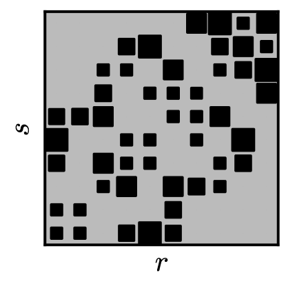
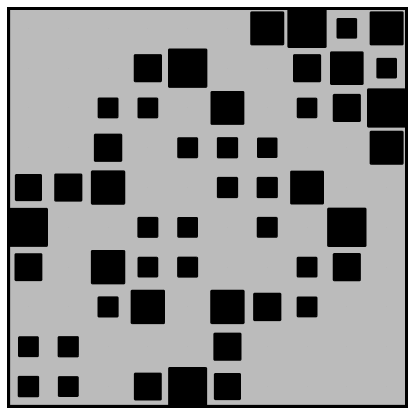
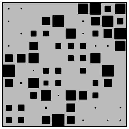
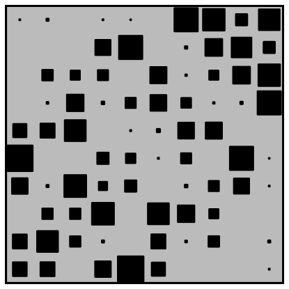
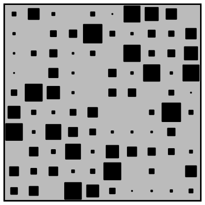
(a) Planted ${\left<k\right>}=15$ ${\left<k\right>}=6$ ${\left<k\right>}=5$ ${\left<k\right>}=4$ Inferred

\begin{overpic}[unit=1mm,width=216.81pt,trim=2.84544pt 0.0pt 0.0pt 0.0pt,clip]{DL-vs-Bmin-benchmark-B10-N10000-S-0_767528364331-deg_corrTrue.pdf} \put(3.0,8.0){(b)} \end{overpic}

\begin{overpic}[unit=1mm,width=216.81pt,trim=7.0563pt 0.0pt 8.5359pt 0.0pt,clip]{MI-vs-Bmin-benchmark-B10-N10000-S-0_767528364331-deg_corrTrue.pdf} \put(3.0,8.0){(c)} \end{overpic}

\begin{overpic}[unit=1mm,width=216.81pt,trim=6.82881pt 0.0pt 1.42271pt 0.0pt,clip]{MI-vs-ak-benchmark-B10-N10000-nsweep2000-deg_corrTrue-escape.pdf} \put(3.0,8.0){(d)} \end{overpic}

Figure 1: (a) Prescribed block structure with $B=10$ and $\mathcal{I}_{t}=\ln B/6$, together with inferred parameters for different ${\left<k\right>}$; (b) Description length $\Sigma_{b}/E$ for different $B$ and ${\left<k\right>}$, for networks sampled from (a). The vertical line marks the position of the global minimum; (c) NMI between the true and inferred partitions, for the same networks as in (b); (d) Same as (b) for different ${\left<k\right>}$ and prescribed block structures. The grey lines correspond to the threshold of Eq. 7. In all cases we have $N=10^{4}$.

MDL bound on detectability — The difference $\Sigma_{b}\equiv\Sigma_{t/c}-\Sigma_{t/c}|_{B=1}$ of the description length of a graph with some block structure and a random graph with $B=1$ can be written as

$$\Sigma_{b}=Eh\left(\frac{B(B+1)}{2E}\right)+N\ln B-E\mathcal{I}_{t/c},$$ (6)

with $\mathcal{I}_{t}=\sum_{rs}m_{rs}\ln(m_{rs}/w_{r}w_{s})$ and $\mathcal{I}_{c}=\sum_{rs}m_{rs}\ln(m_{rs}/m_{r}m_{s})$, where $m_{rs}=e_{rs}/2E$ and $w_{r}=n_{r}/N$ (and equivalently for directed graphs, with $B(B+1)/2\to B^{2}$). We note that $\mathcal{I}_{t/c}\in[0,\ln B]$. If for any given graph we have $\Sigma_{b}>0$, the inferred block structure will be discarded in favor of the simpler fully random $B=1$ model. Therefore the condition $\Sigma_{b}<0$ yields a limit on the detectability of prescribed block structures according to the MDL criterion. For the special case where $E\gg B^{2}$, this inequality translates to a more convenient form,

$${\left<k\right>}>\frac{2\ln B}{\mathcal{I}_{t/c}}.$$ (7)

The directed case is analogous, with $2\ln B\to\ln B$ replaced in the equation above.

Partial detectability and parsimony — The condition $\Sigma_{b}<0$ is not a statement on the absolute detectability of a given model, only to what extent the extracted information (if any) can be used to compress the data. Although these are intimately related, the MDL criterion is based on the idea of perfect (or lossless) compression, and thus corresponds simply to a condition necessary (but not sufficient) for the perfect recoverability of the model parameters from the data. Perfect inference, however, is only possible in the asymptotically dense case ${\left<k\right>}\to\infty$ Decelle et al. (2011b), and in practice one always has some amount of uncertainty. Therefore it remains to be determined how practical is the parsimony limit derived from MDL to establish a noise threshold on empirical data. In Fig. 1 is shown an example of a block structure with $B=10$ and $\mathcal{I}_{t}=\ln B/6$. In Fig. 1b is shown the minimum of $\Sigma_{b}/E$ as function of $B$, for sampled networks with different ${\left<k\right>}$, obtained with the Monte Carlo algorithm described below. If ${\left<k\right>}$ is large enough (${\left<k\right>}>6$, according to Eq. 7), the minimum of $\Sigma_{b}$ is clearly at the correct $B=10$ value, and as is show in Fig. 1b this is exactly where the normalized mutual information (NMI)  between the known and inferred partition is the largest. However, for ${\left<k\right>}<6$ the minimum of $\Sigma_{b}$ is no longer at $B=10$, and instead it is at $B=1$. Nevertheless, the overlap with the correct partition is overall positive and is still is the largest at $B=10$, so the correct partition is to some extent detectable, but the MDL criterion rejects it. By experimenting with different planted block structures (see Fig. 1d), one observes that the MDL threshold lies very close to the parameter region where inferred partition is no longer well correlated with the true partition. This comparison can be made in more detail by considering the special case known as the planted partition model (PP) Condon and Karp (2001), which imposes a diagonal block structure given by $m_{rr}=c/B$, $m_{rs}=(1-c)/B(B-1)$ for $r\neq s$, and $w_{r}=1/B$, and $c\in[0,1]$ is a free parameter. In this case it can be shown that even partial inference is only possible if ${\left<k\right>}>((B-1)/(cB-1))^{2}$ Decelle et al. (2011a, b); Mossel et al. (2012); Nadakuditi and Newman (2012), otherwise no information at all on the original model can be extracted . For smaller values of $B$, this bound is higher than Eq. 7 for this model (where we have $\mathcal{I}_{t/c}=c\ln(Bc)+(1-c)\ln(B(1-c)/(B-1)$), which means that there is a region of parameters where the MDL criterion discards potentially useful (albeit clearly noisy) information (see Fig. 2a). Interestingly, however, for larger values of $B$, the MDL criterion will most often result in lower bounds (see Fig. 2b), meaning that whatever partial information which can be recovered from the model will not be discarded. For $B\to\infty$ we have $c^{*}_{\text{MDL}}\simeq 2/{\left<k\right>}$ and $c^{*}\simeq 1/\sqrt{{\left<k\right>}}$, and thus $c^{*}_{\text{MDL}}<c^{*}$ for ${\left<k\right>}>4$ . Therefore, so far as the PP model serves as a good representation of more general block structures, one should not expect excessive parsimony from MDL, at least for sufficiently large values of $B$.

\begin{overpic}[unit=1mm,width=106.23808pt,trim=7.11317pt 0.0pt 2.56064pt 0.0pt,clip]{MI-vs-cbenchmark-simple-B10-N10000-nsweep5000-deg_corrTrue-mcFalse.pdf} \put(3.0,8.0){(a)} \end{overpic}

\begin{overpic}[unit=1mm,width=106.23808pt,trim=3.41418pt 0.0pt 1.42271pt 0.0pt,clip]{cdiff-vs-ak.pdf} \put(3.0,8.0){(b)} \end{overpic}

Figure 2: (a) NMI between the true and inferred partitions for PP samples with $B=10$ as a function of $c$ for different ${\left<k\right>}$. The grey (red) lines correspond to the threshold $c^{*}$ of Ref. Decelle et al. (2011a) ($c^{*}_{\text{MDL}}$ given by Eq. 7); (b) Difference between $c^{*}_{\text{MDL}}$ and $c^{*}$, for different ${\left<k\right>}$ and $B$.

The largest detectable value of B — The MDL approach imposes an intrinsic constraint on the maximum value of $B$ which can be detected, $B_{\text{max}}$, given a network size and density. This can be obtained by minimizing $\Sigma_{b}$ over all possible block structures with a given $B$, which is obtained simply by replacing $\mathcal{I}_{t/c}$ by its maximum value $\ln B$ in Eq. 6,

$$\Sigma^{\prime}_{b}=Eh\left(\frac{B(B+1)}{2E}\right)-(E-N)\ln B.$$ (8)

Eq. 8 is a strictly convex function on $B$. This means there is a global minimum $\Sigma^{\prime}_{b}|_{B=B_{\text{max}}}$ given uniquely by $N$ and $E$. It is easy to see that even if the prescribed block structure with some $B>B_{\text{max}}$ has minimal entropy (i.e. $\mathcal{I}_{t/c}=\ln B$), alternative partitions with $B^{\prime}<B$ blocks (obtained by merging blocks such that $\mathcal{I}^{\prime}_{t/c}=\ln B^{\prime}$) will necessarily possess a smaller $\Sigma^{\prime}_{b}$. Imposing $\partial\Sigma^{\prime}_{b}/\partial B=0$, one obtains $B_{\text{max}}\cong\mu({\left<k\right>})\sqrt{E}$, with $\mu({\left<k\right>})$ being the solution of $\mu\ln(2/\mu^{2}+1)-(1-1/{\left<k\right>})/\mu=0$ [for the directed case we make $2/\mu^{2}\to 1/\mu^{2}$ and $1/{\left<k\right>}\to 2/{\left<k\right>}$]. Therefore, according to the MDL criterion, the maximum number of blocks which is detectable scales as $B_{\text{max}}\sim\sqrt{N}$ for a fixed value of ${\left<k\right>}$. This is consistent with detectability analysis in Ref. Choi et al. (2012) for traditional blockmodel variant, which showed by other means that the model parameters can only be recovered if $B$ does not scale faster than $\sqrt{N}$. Note that this means that the limit $E\gg B^{2}$ cannot be taken a priori when inferring from empirical data, and hence the value of $\mathcal{L}_{t}$ computed in Ref. Rosvall and Bergstrom (2007) needs to be replaced with Eq. 4 in the general case.

The limit $B_{\text{max}}\propto\sqrt{E}$ is very similar to the so-called “resolution limit” of community detection via modularity optimization Fortunato and Barthélemy (2007), which is $B^{Q}_{\text{max}}=\sqrt{E}$. These two limits, however, have different interpretations: The value of $B^{Q}_{\text{max}}$ arises simply from the definition of modularity, which can be to some extent alleviated (but not entirely avoided) by properly modifying the modularity function with scale parameters Reichardt and Bornholdt (2006); Kumpula et al. (2007); Arenas et al. (2008); Lancichinetti and Fortunato (2011); Xiang and Hu (2011); Ronhovde and Nussinov (2012). On the other hand the value of $B_{\text{max}}$ has a more fundamental character, and corresponds to the situation where knowledge of the complete block structure is no longer the best option to compress the data. This value can be improved only if any a priori information is known which leads to a smaller class of models to be inferred, and hence smaller $\mathcal{L}_{t}$. In general, if we have $\mathcal{L}_{t}=Ef(B^{\alpha}/E)+N\ln B$, where $f(x)$ is any (differentiable) function, performing the same analysis as above leads to $B_{\text{max}}=(\mu(k)E)^{1/\alpha}$, with $\alpha f^{\prime}(\mu)\mu+2/{\left<k\right>}-1=0$. However, it should also be noted that if the existing block structure is locally dense (i.e. $e_{rs}\sim n_{r}n_{s}$), as the union of $B$ complete graphs considered in Fortunato and Barthélemy (2007), the expressions in Eqs. 1 and 2 are no longer valid, and will overestimate the entropy. Using the correct entropy (Eqs. 5 and 9 in Peixoto (2012)) will lead to an improved resolution. Unfortunately, for the dense case, the entropy for the degree-corrected variant cannot be computed in a closed form Peixoto (2012).

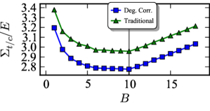
\begin{overpic}[unit=1mm,width=173.44865pt,trim=0.0pt 0.0pt 0.0pt 28.45274pt,clip]{football-profile-deg_corrTrue-graph-best.pdf} \put(-5.0,8.0){(a)} \end{overpic}

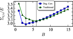
\begin{overpic}[unit=1mm,width=173.44865pt,trim=0.0pt 0.0pt 0.0pt 28.45274pt,clip]{polbooks-profile-deg_corrTrue-graph-best.pdf} \put(3.0,8.0){(b)} \end{overpic}

Figure 3: Top: Value of $\Sigma_{b}/E$ for both blockmodel variants as a function of $B$ for (a) the American football network of Girvan and Newman (2002) (with the corrections described in Evans (2010, 2012)) and (b) the political books network of Krebs . Bottom: Inferred partitions with the smallest $\Sigma_{b}$. Nodes circled in red do not match the known partitions.

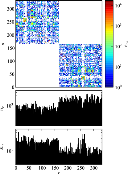
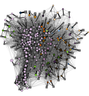
Figure 4: Left: Inferred block structure for the IMDB network, with $N=372,787$, $E=1,812,657$ and $B=332$, according to the MDL criterion, and the degree-corrected stochastic blockmodel. Right: Circles correspond to film blocks, and squares to actors. The node colors correspond to the countries of production. See Supplemental Material for more details.

Detection algorithm — For a fixed $B$, the best partition can be found by minimizing $\mathcal{S}_{t/c}$, via well-established methods such as Markov chain Monte Carlo (MCMC), using the the Metropolis-Hastings algorithm Metropolis et al. (1953); Hastings (1970). However, a naïve implementation based on fully random block membership moves can be very slow. We found that the performance can be drastically improved by using local information and current knowledge of the partially inferred block structure, simply by proposing moves $r\to s$ with a probability $p(r\to s|t)\propto e_{ts}+1$, where $t$ is the block label of a randomly chosen neighbor of the node being moved. Each sweep of this algorithm can be performed in $O(E)$ time, independent of $B$ (see Supplemental Material). Having obtained the minimum of $\mathcal{S}_{t/c}$, the best value of $B$ is obtained via an independent one-dimensional minimization of $\Sigma_{b}$, using a Fibonacci search Press et al. (2007), based on subsequent bisections of an initial interval which brackets the minimum. This method finds a local minimum in $O(\ln B_{\text{max}})$ time. The overall number of steps necessary for the entire algorithm is $O(\tau E\ln B_{\text{max}})$, where $\tau$ is the average mixing time of the Markov chain. If we have no prior information on $B_{\text{max}}$, we need to assume $B_{\text{max}}\sim\sqrt{E}$, in which case the complexity becomes $O(\tau E\ln E)$, or $O(\tau N\ln N)$ for sparse graphs. This compares favorably to minimization strategies which require the computation of the full marginal probability $\pi^{i}_{r}$ that node $i$ belongs to block $r$, such as Belief-Propagation (BP) Decelle et al. (2011a, b); Yan et al. (2012), which results in a larger complexity of $O(NB^{2})$ per sweep (or $O(NB^{2}l)$ for the degree-corrected variant, with $l$ being the number of distinct degrees Yan et al. (2012)), or $O(N^{2})$ for $B\sim B_{\text{max}}$.

Empirical networks — The MDL approach yields convincing results for many empirical networks, as can be seen in Fig. 3, which shows results for the College Football network of Girvan and Newman (2002) and the Political Books network of Krebs . In both cases the correct number blocks is inferred, and the best partition matches reasonably well the known true values, at least for the degree-corrected variant. Employing the Monte Carlo algorithm above, results may be obtained for much larger networks. We show in Fig. 4 the obtained block partition with the degree-corrected variant for the IMDB network of actors and films , where a film node is connected to all its cast members. The bipartiteness of the network is fully reflected in the inferred block partition, where films and actors always belong to different blocks, although this has not been imposed a priori (something which would be impossible to obtain with, e.g. modularity optimization). Besides this role separation, the film blocks are divided sharply along spatial, temporal and genre lines, and the actor blocks are closely correlated with such film classes (see Supplemental Material for a more detailed analysis).

In summary, we showed how minimizing the full description length of empirical network data enables simple, efficient, unbiased and fully non-parametric analysis of the large-scale properties of large networks, for which no a priori information is available, while at the same time providing general bounds on the decodability of arbitrary block structures from empirical data.

See pages - of sup_material.pdf