Role Mining with Probabilistic Models

Abstract

Role mining tackles the problem of finding a role-based access control (RBAC) configuration, given an access-control matrix assigning users to access permissions as input. Most role mining approaches work by constructing a large set of candidate roles and use a greedy selection strategy to iteratively pick a small subset such that the differences between the resulting RBAC configuration and the access control matrix are minimized. In this paper, we advocate an alternative approach that recasts role mining as an inference problem rather than a lossy compression problem. Instead of using combinatorial algorithms to minimize the number of roles needed to represent the access-control matrix, we derive probabilistic models to learn the RBAC configuration that most likely underlies the given matrix.

Our models are generative in that they reflect the way that permissions are assigned to users in a given RBAC configuration. We additionally model how user-permission assignments that conflict with an RBAC configuration emerge and we investigate the influence of constraints on role hierarchies and on the number of assignments. In experiments with access-control matrices from real-world enterprises, we compare our proposed models with other role mining methods. Our results show that our probabilistic models infer roles that generalize well to new system users for a wide variety of data, while other models’ generalization abilities depend on the dataset given.

1 Introduction

Role-Based Access Control (RBAC) [12] is a popular access control model. Rather than directly assigning users to permissions for using resources, for example via an access control matrix, in RBAC one introduces a set of roles. The roles are used to decompose a user-permission relation into two relations: a user-role relation that assigns users to roles and a role-permission relation that assigns roles to permissions. Since roles are (or should be) natural abstractions of functional roles within an enterprise, these two relations are conceptually easier to work with than a direct assignment of users to permissions. Experience with RBAC indicates that this decomposition works well in practice and facilitates the administration of large-scale authorization policies for enterprises with many thousands of users and permissions.

Although the benefits of using RBAC are widely recognized, its adoption and administration can be problematic in practice. Adoption requires that an enterprise migrates its authorizations to RBAC. Additionally, even after RBAC is in place, authorizations may need to be reassigned after major changes within the enterprise, for example, after a reorganization or a merger where processes and IT systems from different divisions must be consolidated. Migration and the need to reengineer roles after major changes are the most expensive aspects of RBAC.

To address these problems, different approaches have been developed to configuring RBAC systems. These approaches have been classified into two kinds [37]: top-down and bottom-up role engineering. Top-down engineering configures RBAC independently of any existing user-permission assignments by analyzing the enterprise’s business processes and its security policies. Bottom-up role-engineering uses existing user-permission assignments to find a suitable RBAC configuration.

When carried out manually, bottom-up role engineering is very difficult and therefore incurs high costs and poses security risks. To simplify this step, [24] proposed the first automatic method for bottom-up role engineering and coined the term role mining for such methods. Numerous role mining algorithms have been developed since then, notably [9, 35, 26, 31, 38].

Unfortunately, most role mining algorithms suffer from the drawback that the discovered roles are artificial and unintuitive for the administrators who must assign users to roles. This undesirable effect is linked to the design principle for role mining algorithms that aim at achieving one of the following two goals:

• minimizing the deviation between the RBAC configuration and the given access control matrix for a given number of roles, or

• minimizing the number of roles for a given deviation (possibly zero).

Both goals amount to data compression. As a result, the roles found are often synthetic sets of permissions. Although these roles minimize the RBAC configuration, they are difficult to interpret as functional roles, also called business roles, that reflect the business attributes of the users assigned to them. This shortcoming not only limits the acceptance of the new RBAC configuration among employees, it also makes the RBAC configuration difficult to maintain, for example, to update when users join the system or change their business role within the enterprise. Moreover, by optimizing the roles to fit existing authorizations as close as possible, existing erroneous user-permission assignments are likely to be migrated to the new RBAC system. Several attempts have been made to incorporate business attributes into the role mining process to improve the business-relevance of the roles [29, 18]. However, these algorithms compress the access control matrix as the underlying objective and they do not necessarily infer predictive roles.

The problems outlined above arise because the predominant definitions of the role mining problem [36, 20, 25, 27] do not reflect realistic problem settings. In particular, all prior definitions assume the existence of input that is usually not available in practice. For example, the input includes either the number of roles to be found or the maximally tolerable residual error when fitting the RBAC configuration to the given access-control matrix. Guided by these definitions, the respective algorithms focus on compressing user-permission assignments rather than on structured predictions of roles. However, compression addresses the wrong problems. We argue that there is a need for a definition of role mining as an inference problem that is based on realistic assumptions. Consequently, given such a definition, algorithms must be developed that aim at solving this problem. Moreover it is necessary to have quality measures to compare how well different algorithms solve the problem. Our contributions cover all these aspects:

• We provide the first complete approach to probabilistic role mining, including the problem definition, models and algorithms, and quality measures.

• We define role mining as an inference problem: learning the roles that most likely explain the given data. We carefully motivate and explicate the assumptions involved.

• We propose probabilistic models for finding the RBAC configuration that has most likely generated a given access-control matrix.

• We demonstrate that the RBAC configuration that best solves the role inference problem contains roles that generalize well to a set of hold-out users. We therefore provide a generalization test to evaluate role mining algorithms and apply this test to our methods and to competing approaches.

• We experimentally demonstrate that our probabilistic approach provides a sound confidence estimate for given user-permission assignments.

• We develop a hybrid role mining algorithm that incorporates business attributes into the role mining process and thereby improves the interpretability of roles.

We proceed as follows. First, in Section 2, we review the assumptions that are often implicitly made for role mining and we use them to define the inference role mining problem together with appropriate evaluation criteria. Then, in Section 3, we derive a class of probabilistic models from the deterministic user-permission assignment rule of RBAC. We explain two model instances in detail and we propose learning algorithms for them in Section 4. In Sections 5, we report on experimental findings on real world access control data. In Section 6, we show how to include business attributes of the users in the role mining process to obtain a hybrid role mining algorithm and we experimentally investigate how these attributes influence the RBAC configurations discovered. We discuss related work in Section 7 and draw conclusions in Section 8

2 Problem definition

In this section we define the role inference problem. First, we explain the assumptions underlying our definition. Afterwards we present a general definition of role mining that takes business-relevant information into account. The pure bottom-up problem without such information will be a special case of the general problem. Finally, we propose quality measures for assessing role mining algorithms.

Figure 1: Graphical illustration of the decomposition of an access control matrix $\mathbf{X}$, which assigns $N$ users to $D$ permissions, into an RBAC configuration with two assignments: $\mathbf{Z}$ assigns users to $K$ roles and $\mathbf{U}$ assigns roles to permissions. The reconstruction $\mathbf{Z}\ast\mathbf{U}$ fits $\mathbf{X}$ up to residuals. The Boolean matrices $\mathbf{X}$, $\mathbf{Z}$, and $\mathbf{U}$ encode the relations $U\!P\!A$, $U\!A$, and $P\!A$, respectively.

2.1 Assumptions and problem definition

The role mining problem is defined in terms of a set of users $U\mspace{-0.9mu}S\mspace{-0.9mu}E\mspace{-0.9mu}R\mspace{-0.7mu}S$, a set of permissions $P\mspace{-0.9mu}R\mspace{-0.9mu}M\mspace{-0.9mu}S$, a user-permission assignment relation $U\!P\!A$, a set of roles $RO\mspace{-0.9mu}L\mspace{-0.9mu}E\mspace{-0.9mu}S$, a user-role assignment relation $U\!A$, a role-permission assignment relation $P\!A$, and, if available, top-down information $T\!DI$. Our problem definition is based on three assumptions about the relationships between these entities and the generation process of $U\!P\!A$. All these entities and their relationships are sketched in Figure 2.

Assumption 1: An underlying RBAC configuration exists

We assume that the given user-permission assignment $U\!P\!A$ was induced by an unknown RBAC configuration $RC^{*}\!\!=\!(RO\mspace{-0.9mu}L\mspace{-0.9mu}E\mspace{-0.9mu}S^{*}\!\!,U\!A^{*}\!\!,P\!A^{*})$, where “induced” means that $U\!P\!A\approx U\!A^{*}\ast P\!A^{*}$. This assumption is at the heart of role mining. To search for roles implicitly assumes that they are there to be found. Said another way, searching for roles in direct assignments between users and permissions only makes sense if one assumes that parts of the data could, in principle, be organized in such a structured way. Without this assumption, the role structure that one can expect to find in a given access-control matrix would be random and therefore meaningless from the perspective of the enterprise’s business processes and security policies.

Assumption 2: Top-down information $T\!DI$ influences the RBAC configuration $RC^{*}$

We assume that $RC^{*}$ reflects the enterprise’s security policies and the business processes in the sense that $RC^{*}$ encodes these policies and enables users to carry out their business tasks. Full knowledge of the security policies and business processes, as well as all business attributes and user tasks, should, in principle, determine the system’s user-permission assignment. We denote all such information as top-down information (TDI); this name reflects that the task of configuring RBAC using TDI is usually referred to as top-down role mining. In practice, only parts of TDI may be available to the role mining algorithm. In Figure 2, we account for this structure by distinguishing “TDI” from “TDI input”. Whenever some parts of TDI are used in the role mining process we then speak of hybrid-role mining.

Assumption 3: Exceptions exist

The observed user-permission assignment $U\!P\!A$ might contain an unknown number of exceptions. An exception is a user-permission assignment that is not generated by the role-structure $RC^{*}$ but rather from a set of unknown perturbation processes. To capture this assumption in Figure 2, we distinguish the given access control matrix $U\!P\!A\approx U\!A^{*}\ast P\!A^{*}$ from an unknown exception-free matrix $U\!P\!A^{\prime}=U\!A^{*}\ast P\!A^{*}$ that is fully determined by the role structure. We emphasize that, even though there are many ways errors can arise in a system, exceptions are not necessarily errors. Moreover, a role mining algorithm cannot be expected to discriminate between an error (that is, an unintended exception) and an intentionally made exception, if additional information is not provided. A role mining algorithm can identify exceptions and report them to a domain expert (ideally ranked by their likelihood). Such a procedure already provides a substantial advantage over manually checking all user-permission pairs as it involves far fewer checks. Due to the lack of additional information, we abstain from making further assumptions about the exceptions, for instance the fraction of exceptions $\delta$. Instead, determining such parameters will constitute an important part of the role mining problem.

We now propose the following definition of the role mining problem.

Definition 1.

Role inference problem
Let a set of users $U\mspace{-0.9mu}S\mspace{-0.9mu}E\mspace{-0.9mu}R\mspace{-0.7mu}S$, a set of permissions $P\mspace{-0.9mu}R\mspace{-0.9mu}M\mspace{-0.9mu}S$, a user-permission relation $U\!P\!A$, and, optionally, parts of the top-down information $T\!DI$ be given. Under Assumptions 1–3, infer the unknown RBAC configuration $RC^{*}\!\!=\!(RO\mspace{-0.9mu}L\mspace{-0.9mu}E\mspace{-0.9mu}S^{*}\!\!,U\!A^{*}\!\!,P\!A^{*})$.

This definition, together with the assumptions on $U\!P\!A$’s generation process, provides a unified view of bottom-up and hybrid role mining. The two cases only differ in terms of the availability of top-down information $T\!DI$. In hybrid role mining, parts of the top-down information that influenced $RC^{*}$ is available. When $T\!DI$ is not provided, the problem reduces to bottom-up role mining. Note that in such cases the goal still remains the same: the solution to Problem 1 solves the bottom-up problem as well as the hybrid role mining problem. Thereby, the assumption that $RC^{*}$ is (partially) influenced by $T\!DI$ is also reasonable for the pure bottom-up role mining problem. Whether $T\!DI$ actually influences $RC^{*}$ does not depend on the availability of such data.

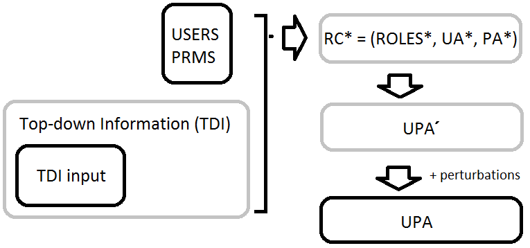
Figure 2: Dependencies of the entities involved in role mining. This scheme illustrates how the user-permission assignment $U\!P\!A$ is assumed to be generated. An arrow indicates the direction of the generation process. Grey entities are unknown and black ones are given as input. For pure bottom-up role mining, no top-down information is given.

Relationship to role mining by compression

The role mining problems that aim to achieve the closest fit for a given compression ratio or achieve the best compression for a given deviation differ from the role inference problem. Technically, our definition has less input than the alternatives. For the above-mentioned problems, either the number of roles $k$ or the deviation $\delta$ is provided as input. In contrast, our definition makes no assumptions on these quantities and both $k$ and $\delta$ must be learned from $U\!P\!A$ (as finding $RC^{*}$ involves finding $k$ and, at the same time, determines $\delta=U\!P\!A-U\!A^{*}\ast P\!A^{*}$).

Moreover, we see it is an advantage that the assumptions of the problem are explicitly given. By making the assumption of an underlying role structure a condition for role mining, our problem definition favors conservative algorithms in the following sense. If little or no structure exists in $U\!P\!A$, the optimal algorithm should refrain from artificially creating too many roles from $U\!P\!A$. In contrast, if the number of roles or the closeness of fit is predetermined, optimal algorithms will migrate exceptional (and possibly unwarranted) permissions to RBAC.

Finally, it is unrealistic in practice that $\delta$ or $k$ will be given as an input. Hence, treating them as unknowns reflects real-world scenarios better than previous definitions for role mining that require either $\delta$ or $k$ as inputs.

2.2 Quality measures

Comparison with true roles

The obvious quality measure that corresponds to the role inference problem is the distance to the hidden RBAC configuration $RC^{*}$ underlying the given data $U\!P\!A$. Several distance metrics for comparing two RBAC configurations exist, for instance the Hamming distance between the roles or the Jaccard similarity between the roles. Usually, however, $RC^{*}$ is not known in practice. A comparison is possible only for artificially created user-permission assignments where we know $RC^{*}$ or when an existing RBAC configuration is used to compute a user-permission assignment. We therefore focus in this paper on quality measures that are applicable to all access control matrices, independent of knowledge of $RC^{*}$.

Generalization error

We propose to use generalization error for evaluating RBAC configurations. The generalization error is often used to assess supervised learning methods for prediction [21]. The generalization error of an RBAC configuration $RC$ that has been learned from an input dataset $\mathbf{X}^{(1)}$ indicates how well $RC$ fits to a second dataset $\mathbf{X}^{(2)}$ that has been generated in the same way as $\mathbf{X}^{(1)}$.

Computing the generalization error for an unsupervised learning problem like role mining is conceptually challenging. In general, it is unclear how to transfer the inferred roles to a hold-out test dataset when no labels are given that indicate a relationship between roles and users. We employ a method that can be used for a wide variety of unsupervised learning problems: the transfer costs proposed in [15]. The transfer costs of a role mining algorithm are computed as follows. First the input dataset is randomly split along the users into a training set $\mathbf{X}^{(1)}$ and a validation set $\mathbf{X}^{(2)}$. Then the role mining algorithm learns the RBAC configuration $RC=(\hat{\mathbf{Z}}$, $\hat{\mathbf{U}})$ based only on the training set and without any knowledge of the second hold-out dataset. Having learned $RC$, the solution is transfered to the hold-out dataset by using a nearest neighbor mapping between the users of both datasets. Each user in $\mathbf{X}^{(2)}$ is assigned to the set of roles of its nearest neighbor user in $\mathbf{X}^{(1)}$. Technically, this means we keep $\hat{\mathbf{U}}$ fixed and create a new assignment matrix $\mathbf{Z}^{\prime}$, where row $i$ is copied from the row in $\hat{\mathbf{Z}}$ that corresponds to the nearest neighbor user of user $i$. Then generalization error is the Hamming distance between $\mathbf{Z}^{\prime}\ast\hat{\mathbf{U}}$ and $\mathbf{X}^{(2)}$ divided by the number of entries of $\mathbf{X}^{(2)}$. This ratio denotes the fraction of erroneously generalized assignments.

The rationale behind our measure is intuitive: Since the input dataset is assumed to be generated by an unknown RBAC configuration $RC^{*}$, the subsets $\mathbf{X}^{(1)}$ and $\mathbf{X}^{(2)}$ have also been generated by $RC^{*}$. The structure of the input matrix is the same in different subsets of the dataset, but the random exceptional assignments are unique to each user. A role mining algorithm that can infer $RC^{*}$ from one subset, will have a low generalization error because the generating RBAC configuration should generalize best to the data that it has generated. As a consequence, a role mining algorithm that overfits to noise patterns in one dataset will fail to predict the structure of the second dataset. Thereby, even a perfect role mining algorithm will have a positive generalization error if the data is noisy. It is the relationship to the generalization error of other algorithms that counts. All methods fail to predict exceptional assignments but the better methods will succeed in identifying the structure of the hold-out data while the inferior methods will compromise the underlying structure to adapt to exceptions.

An advantage of computing the generalization error as described above is that this computation is agnostic to the role mining algorithm used. In particular it works for both probabilistic and combinatorial methods. For probabilistic methods one could achieve improved results by using a posterior inference step to assign test users to the roles discovered. However, this method is tailored to the particular methods employed and would not work for methods without a probabilistic model.

3 From a deterministic rule to a class of probabilistic models

In this section we propose a class of probabilistic models for role mining. We derive our core model from the deterministic assignment rule of RBAC and extend this core model to more sophisticated models. We will present two such extensions: (1) the disjoint-decomposition model (DDM) with a two-level role hierarchy where each user has only one role and (2) multi-assignment clustering (MAC), a flat RBAC model featuring a role relationship where users can assume multiple roles. We will also show why these two instances of the model class are particularly relevant for role mining.

3.1 Core model

In the following, we derive the core part of our probabilistic model. We start with the deterministic rule that assigns users to permissions based on a given role configuration. We then convert this rule into a probabilistic version, where one reasons about the probability of observing a particular user-permission assignment matrix given the probabilities of users having particular roles and roles entailing permissions.

We denote the user-permission assignment matrix by $\mathbf{X}$, with $\mathbf{X}\in\{0,1\}^{N\times D}$. As short-hand, we write $\mathbf{x}_{i\ast}$ for the $i^{\textrm{th}}$ row of the matrix and $\mathbf{x}_{\ast d}$ for the $d^{\textrm{th}}$ column. We define the generative process of an assignment $x_{id}\in\left\{0,1\right\}$ by

$$u_{kd} \sim p(u_{kd}|\beta_{kd})$$ (1)

$$x_{id} \sim p(x_{id}|\mathbf{u}_{\ast d},\mathbf{z}_{i\ast})\,,$$ (2)

where $a\sim p(a)$ means that $a$ is a random variable drawn from the probability distribution $p(a)$. The latent variable $u_{kd}\in\left\{0,1\right\}$ determines permission ${d}\in\left\{1,...,D\right\}$ of source $k\in\left\{1,...,K\right\}$. The parameter $z_{ik}\in\left\{0,1\right\}$ encodes whether user $i$ is assigned to role $k$. As $u_{kd}$ is binary, $p(u_{kd}|\beta_{kd})$ is a Bernoulli distribution, with $p(u_{kd}=0):=\beta_{kd}$ and

$$p(u_{kd}|\beta_{kd}):=\beta_{kd}^{1-u_{kd}}(1-\beta_{kd})^{u_{kd}}\,.$$ (3)

Throughout this section, we will condition all probabilities on $\mathbf{Z}$. Therefore, we can ignore $p(z_{ik})$ for the moment and treat it as a model parameter here. In Section 3.3 we will treat $z_{ik}$ as a random variable and describe a particular prior distribution for it.

The generative model that we described so far is illustrated in Figure 3. All entities in this figure have a well-defined semantic meaning. The circles are random variables. A filled circle denotes that the variable is observable (like the user-permission assignment $x_{id}$) and an empty circle represents a hidden variable. Small solid dots are unknown model parameters. Arrows indicate statistical dependencies between entities. Whenever an entity is in a rectangle (say in the $N$-rectangle and in the $D$-rectangle) then multiple different realizations of this entity exist (here $N\cdot D$ realizations of $x_{id}$, each with a different index $i$ and $d$).

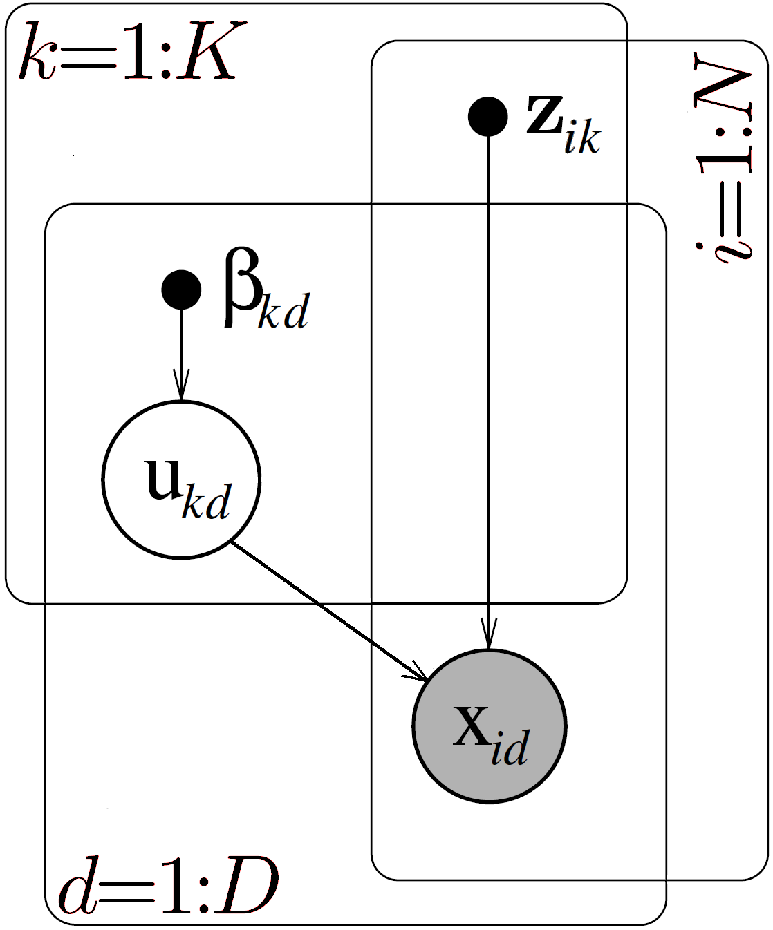
Figure 3: Graphical model corresponding to the generation rule of user-permission assignments given an RBAC configuration. See the explanation of the semantics in the text.

The probability $p(x_{id}|\mathbf{u}_{\ast d},\mathbf{z}_{i\ast})$ is deterministic in the following sense. Given all role-permission assignments $\mathbf{u}_{kd}$ and the role assignments $\mathbf{z}_{i\ast}$, the bit $x_{id}$ is determined by the disjunction rule defined by the Boolean matrix product

$$\mathbf{X}=\mathbf{Z}\ast\mathbf{U}\ \ \ \text{such that}\ \ \ \ \ \ x_{id}=f(\mathbf{u}_{\ast d},\mathbf{z}_{i\ast}):=\bigvee_{k=1}^{K}\left(z_{ik}\wedge u_{kd}\right)\ .$$ (4)

To derive the likelihood of $x_{id}$, we express this deterministic formula $x_{id}=f(\mathbf{u}_{\ast d},\mathbf{z}_{i\ast})$ in terms of a probability distribution. To this end, the entire probability mass must be concentrated at the deterministic outcome, i.e. the distribution must be of the form

$$p(x_{id}|\mathbf{u}_{\ast d},\mathbf{z}_{i\ast})=\left\{\begin{array}[]{cl}1,&\mbox{if }x_{id}=f(\mathbf{u}_{\ast d},\mathbf{z}_{i\ast})\\ 0,&\mbox{otherwise}\end{array}\right.\,.$$ (5)

A probability distribution that fulfills this requirement is

$$p(x_{id}|\mathbf{u}_{\ast d},\mathbf{z}_{i\ast})=\Bigl{(}\prod_{k}\left(1-u_{kd}\right)^{z_{ik}}\Bigr{)}^{(1-x_{id})}\Bigl{(}1-\prod_{k}\left(1-u_{kd}\right)^{z_{ik}}\Bigr{)}^{x_{id}}.$$ (6)

This can be seen by going through all eight combinations (for a single $k$) of the binary values of $z_{ik}$, $x_{id}$, and $u_{kd}$. The distribution reflects that there are only two possible outcomes of this random experiment. In the following, we exploit this property and work just with probabilities for $x_{id}=0$. The probability for $x_{id}=1$ is always the remaining probability mass.

The model in its current deterministic state is not directly useful for role mining given the hidden variables $u_{kd}$. We therefore eliminate the $u_{kd}$ to obtain a likelihood that only depends on the model parameters and the observations. This can be achieved by marginalizing out $u_{kd}$, i.e., summing over all possible $K\times D$ matrices $\mathbf{u}$. As derived in Appendix A.1, this yields the likelihood $p(x_{id}=0|\boldsymbol{\beta}_{\ast d},\mathbf{z}_{i\ast})=\prod_{k}\beta_{kd}^{z_{ik}}$. This term reflects that if a user is not assigned to a role, then the role does not have any influence on the user’s permissions. Therefore, the chance of a user not being assigned some permission $d^{\prime}$ decreases with the number of roles of the user, since the chances $\beta_{kd^{\prime}}$ of $d^{\prime}$ not being assigned to the roles are multiplied.

As $x_{id}$ can only take two possible values, we have $p(x_{id}=1|\boldsymbol{\beta}_{\ast d},\mathbf{z}_{i\ast})=1-\prod_{k}\beta_{kd}^{z_{ik}}$ such that the full likelihood of the bit $x_{id}$ is

$$p(x_{id}|\boldsymbol{\beta}_{\ast d},\mathbf{z}_{i\ast})=\left(\prod_{k}\beta_{kd}^{z_{ik}}\right)^{1-x_{id}}\left(1-\prod_{k}\beta_{kd}^{z_{ik}}\right)^{x_{id}}\ .$$ (7)

According to this likelihood, the different entries in $\mathbf{X}$ are conditionally independent given the parameters $\mathbf{Z}$ and $\boldsymbol{\beta}$. Therefore, the complete data likelihood factorizes over users and permissions: $\ p(\mathbf{X}|\boldsymbol{\beta},\mathbf{Z})=\prod_{i=1}^{N}\prod_{d=1}^{D}p(x_{id}|\boldsymbol{\beta}_{\ast d},\mathbf{z}_{i\ast})$.

3.2 Role hierarchies

In this section we extend the core model by introducing role hierarchies. The core model provides a hierarchy of depth 1 as there is only one level of roles. We introduce an additional level, resulting in a hierarchy of depth 2. The meaning of the hierarchical relationship is as follows. Roles in the second layer can be sub-roles of roles in the first layer. The set of permissions for a super-role includes all permissions of its sub-roles.

Our derivation is generic in that it can be used to add extra layers to a hierarchical model. By repeated application, one can derive probabilistic models with hierarchies of any depth. As we will see, the one-level hierarchy (flat RBAC) and the two-level hierarchy are particularly interesting. In Section 3.3 we propose a model variant for flat RBAC and a model variant with a two-level hierarchy.

Like the core model, the hierarchical model derived here is not restricted to role mining. However, we will motivate its usefulness of hierarchies by practical considerations in access-control. We assume that there exists a decomposition of the set of users into partially overlapping groups: Users are assigned to one or more groups by a Boolean assignment matrix $\mathbf{Z}$. Each row $i$ represents a user and the columns $k$ represent user-groups. In practice, such a decomposition may be performed by an enterprise’s Human Resources Department, for example, by assigning users to enterprise divisions according to defined similarities of the employees. If such data is lacking, then the decomposition may just be given by the differences in the assigned permissions for each user. For simplicity, the matrix $\mathbf{Z}$ has the same notation as in the last section.

We now introduce a second layer. We assume that there is a decomposition of the permissions such that every permission belongs to one or more permission-groups. These memberships are expressed by the Boolean assignment matrix $\mathbf{Y}$. Here the $l$th row of $\mathbf{Y}$ represents the permission-group $l$ and the $d$th column is the permission $d$. The assignment of permissions to permission-groups can be motivated by the technical similarities of the resources that the permissions grant access to. For example, in an object-oriented setting, permissions might be grouped that execute methods in the same class. Alternatively, permissions could be categorized based on the risk that is associated with granting someone a particular permission. Of course, permissions can also be grouped according to the users who own them.

We denote user-groups by business roles whereas we call permission-groups technical roles. Business roles are assigned to technical roles. We represent these assignments by a matrix $\mathbf{V}$. To keep track of all introduced variables, we list the types of the above-mentioned Boolean assignment matrices:

$\bullet$	Users $i$ to permissions $d$:	$\!x_{id}\!\in\!\left\{0,1\right\}$, where $i\!\in\!\left\{1,...,\!N\right\},d\!\in\!\left\{1,...,\!D\right\}$.
$\bullet$	Users $i$ to business roles $k$:	$z_{ik}\in\left\{0,1\right\}$, where $k\in\left\{1,...,K\right\}$.
$\bullet$	Business roles $k$ to technical roles $l$:	$v_{kl}\in\left\{0,1\right\}$, where $l\in\left\{1,...,L\right\}$.
$\bullet$	Technical roles $l$ to permissions $d$:	$y_{ld}\in\left\{0,1\right\}$.

Throughout this section, the indices $i$, $d$, $k$, and $l$ have the above scope and are used to index the above items.

Starting with this additional layer of roles, one can recover a flat hierarchy by collapsing the role-role assignment matrix and the role-permission assignments using the disjunction rule $u_{kd}=\bigvee_{l}v_{kl}\wedge y_{ld}$. Thereby, $\mathbf{U}$ can be understood as the role-permission assignment matrix from the last section. With this structure, the final $N\times D$ user-permission assignment matrix $\mathbf{X}$ is determined by two Boolean matrix products

$$\mathbf{X}=\mathbf{Z}\ast\mathbf{U}=\mathbf{Z}\ast\mathbf{V}\ast\mathbf{Y}\ \ \ \text{ with }~{}x_{id}=\bigvee_{k}\left[z_{ik}\wedge\left(\bigvee_{l}v_{kl}\wedge y_{ld}\right)\right]\,.$$ (8)

Equation 8 expresses when a user $i$ is assigned to permission $d$. There exists one Boolean matrix product per role layer. Note that for a given RBAC configuration, we can also partially collapse hierarchies. In particular, this makes sense when a business role is directly linked to permissions. We are again interested in the probability of such an assignment. Starting from this logical expression, we derive below how likely it is to observe an assignment of a user $i$ to a permission $d$.

The deterministic assignment rule for two layers of roles is graphically illustrated in Figure 4(a): a user is assigned to a permission if there is at least one path in the graph connecting them. As this figure indicates, a user can be assigned to a permission in multiple ways, that is, there may be multiple paths. It is therefore easier to express how a user may not be assigned to a permission (we denote this by $\neg x:=\overline{x}$) rather than computing the union over all possible assignment paths. Also, we will abbreviate parameters by $z^{+}\!:=\!p(z\!=\!1)$ and, for independent variables, $\mathbf{z}_{i\ast}^{+}\!:=\!\{z^{+}_{i1},...,z^{+}_{iK}\}$.

$$\hbox to0.0pt{\hss$p$}\left(\overline{x_{id}}\ {|\mathbf{z}_{i\ast}^{+},\mathbf{y}_{\ast d}^{+},V^{+}}\right) = p\left(\overline{\bigvee_{k=1}^{K}\left[z_{ik}\wedge\left(\bigvee_{l=1}^{L}v_{kl}\wedge y_{ld}\right)\right]}\ {|\mathbf{z}_{i\ast}^{+},\mathbf{y}_{\ast d}^{+},V^{+}}\right)$$ (9)

As shown in Appendix A.2, this probability is

$$\hbox to0.0pt{\hss$p$}\left(\overline{x_{id}}\ {|\mathbf{z}_{i\ast}^{+},\mathbf{y}_{\ast d}^{+},V^{+}}\right)={\prod_{k}\left(1-z_{ik}^{+}+z_{ik}^{+}\ \prod_{l}\left(1-y_{ld}^{+})+y_{ld}^{+}(1-v_{kl}^{+})\right)\right)}\,.$$ (10)

We condition this expression on the binary entries of $\mathbf{Y}$ and $\mathbf{Z}$.

$$p(\overline{x_{id}}\left.\right|\mathbf{z}_{i\ast},\mathbf{y}_{\ast d}{,v_{kl}^{+}}) \!=\! \prod_{k}1^{1-z_{ik}}\cdot\left(\prod_{l}{(1-v_{kl}^{+})}^{y_{ld}}\cdot 1^{1-y_{ld}}\right)^{z_{ik}}\!\!=\!\prod_{k,l}{(1-v_{kl}^{+})}^{z_{ik}y_{ld}}$$ (11)

As this expression is independent of other matrix entries in $\mathbf{X}$, we can express the complete likelihood of the user-permission assignment matrix given the business roles and technical roles as a product over users and permissions.

$$p\left(\mathbf{X}\left.\right|\mathbf{Z},\mathbf{Y}\right) =\prod_{i,d}\left[1-p(\overline{x_{id}}\left.\right|\mathbf{z}_{i\ast},\mathbf{y}_{\ast d}{,v_{kl}^{+}})\right]^{x_{id}}\left[p(\overline{x_{id}}\left.\right|\mathbf{z}_{i\ast},\mathbf{y}_{\ast d}{,v_{kl}^{+}})\right]^{1-x_{id}}$$

$$=\prod_{i,d}\left[1-\prod_{k,l}{(1-v_{kl}^{+})}^{z_{ik}y_{ld}}\right]^{x_{id}}\left[\prod_{k,l}{(1-v_{kl}^{+})}^{z_{ik}y_{ld}}\right]^{1-x_{id}}$$ (12)

If we treat $v_{kl}$ as a random variable with probability ${p(v_{kl}=0)=(1-v_{kl}^{+})}$, then this likelihood resembles the one with only one layer of roles. The only differences are the additional binary variables $y_{ld}$ in the exponent that, like $z_{ik}$, can switch off individual terms of the product. Thereby, we chose to condition on $\mathbf{Y}$ and $\mathbf{Z}$ and leave $v_{kl}$ random. We could as well have conditioned on $\mathbf{V}$ and $\mathbf{Z}$ and inferred $y_{ld}$. This alternative points to a generic inference strategy for role hierarchies of arbitrary size. One treats the assignment variables in one layer as a random variable and conditions on the current state of the others. We will demonstrate such an alternating inference scheme on a two level hierarchy in Section 3.3.

3.3 Overparametrization and instantiation by introducing constraints

The above model of user-permission assignments defines a very general framework. In principle, one can iteratively introduce additional layers in the role hierarchy without substantially changing the outer form of the likelihood. In the derivations, we have avoided any prior assumptions on the probabilities of the entries of $\mathbf{V}$, $\mathbf{Y}$, and $\mathbf{Z}$. We have only exploited the fact that these variables are Booleans and, therefore, only take the values 0 or 1. We have also avoided any assumptions about the processes that lead to a particular decomposition of the set of users and the set of permissions. Moreover, we have not specified any constraints on the user decomposition, the permission decomposition, or the assignments from user-groups to permission-groups.

It turns out that the model with a two-level hierarchy already has more degrees of freedom than is required to represent the access control information present in many domains that arise in practice. In particular, when only the data $\mathbf{X}$ is given, there is no information available on how to decompose the second role level. This lack of identifiability becomes obvious when we think about a one-level decomposition with role-permission assignments $\mathbf{U}$ (as in Eq. (4)) and try to convert it into a two-level decomposition. The $\mathbf{Z},\mathbf{U}$ decomposition has already sufficiently many degrees of freedom to fit any binary matrix. Further decomposing $\mathbf{U}$ into an extra layer of roles $\mathbf{V}$ and assignments from these roles to permissions $\mathbf{Y}$ is arbitrary when there does not exist additional information or constraints. Therefore, the flat RBAC configuration with only one role layer is the most relevant one. The two-level hierarchy without constraints is over-parameterized. Such a hierarchy can be seen as a template for an entire class of models. By introducing constraints, we can instantiate this template to specialized models that fit the requirements of particular RBAC environments and have a similar model complexity as flat RBAC without constraints. These instances of the model class are given by augmenting unconstraint two-level RBAC with assumptions on the probability distributions of the binary variables and giving constraints on the variables themselves. In the following, we will present two relevant model instances and explain their relationship. Later, we will extend the models with generation processes for exceptional assignments.

Flat RBAC

In this model, each permission is restricted to be a member of only one permission-group and each permission-group can contain only a single permission. Formally: $\textstyle\left(\forall l:\sum_{j}y_{ld}=1\right)\wedge\left(\forall j:\sum_{l}y_{ld}=1\right)$. The conditioned likelihood then becomes

$$p_{\text{flat}}\left(\mathbf{X}\left.\right|\mathbf{Z}\right)=\prod_{i,d}\left[1-\prod_{k}p(\overline{v_{kd}})^{z_{ik}}\right]^{x_{id}}\left[\prod_{k}p(\overline{v_{kd}})^{z_{ik}}\right]^{1-x_{id}}\hbox to0.0pt{.\hss}$$ (13)

This “collapsed” model is equivalent to flat RBAC without constraints. This can be seen by renaming $v$ by $u$ and $J$ by $D$. As each technical role serves as a proxy for exactly one permission, we have $D=J$ anyway. A graphical representation of the structure of this model instance is given in Figure 4(b). Equivalently, we could introduce one-to-one constraints on the user role assignment and collapse $\mathbf{Z}$ instead of $\mathbf{Y}$, leading to a model with the same structure.

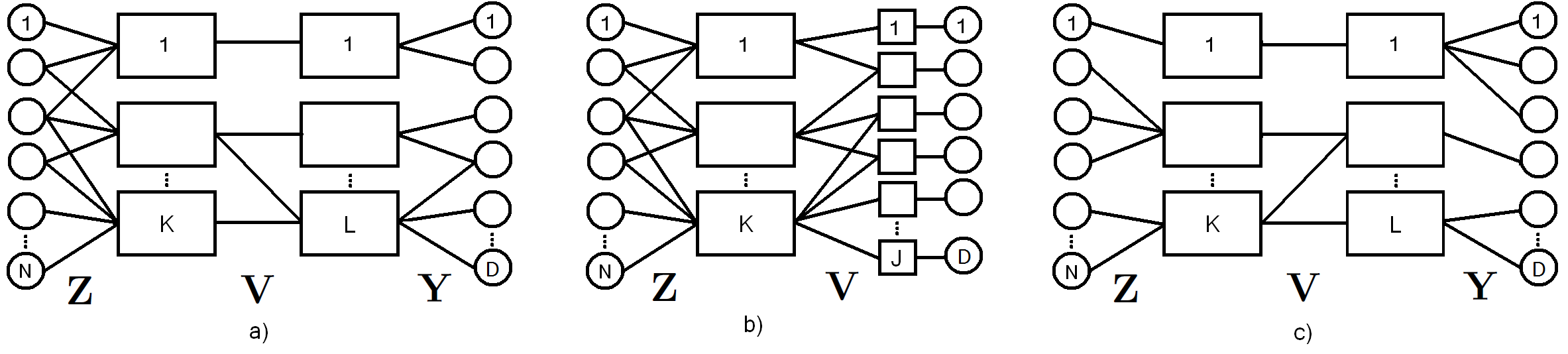
Figure 4: Illustration of the structure of three model instances. A user has a permission if there is at least one path connecting them. a) Full model. b) Model with trivial decomposition of the permissions (flat RBAC). c) Disjoint Decomposition Model with only one business role per user and one technical role per permission.

Disjoint decomposition model (DDM)

This model has even stronger constraints. Namely, $k_{max}=1$ and the number of assigned permission-groups per permission is limited to $l_{max}=1$. This formalizes that each user belongs to exactly one user-group and each permission belongs to exactly one permission-group. Hence, both users and permissions are respectively partitioned into disjoint business roles and technical roles. A disjoint decomposition substantially reduces the complexity of a two-level hierarchy while still retaining a high degree of flexibility since users of a given user-group may still be assigned to multiple permission-groups. We illustrate this model in Figure 4(c).

3.4 Prior assumptions on probabilities

A central question in role mining is how many roles are required to explain a given dataset. In this paper, we take two different approaches to determining the number of roles $k$. For the flat RBAC model, we treat $k$ as a fixed model parameter. One must therefore repeatedly run the algorithm optimizing this model for different $k$ and select the result according to an external measure. In our experiments, we will tune the number of roles $k$ by cross-validation using the generalization error as the external quality measure. For DDM with a two-level hierarchy, we explicitly include prior assumptions on the number of roles into the model using a non-parametric Bayesian approach. This way, the role mining algorithm can internally select the number of roles.

Instead of directly providing the number of roles for DDM, we only assume that, given an RBAC configuration with roles and user-role assignments, the a priori probability of a new user being assigned to one of the roles depends linearly on the number of users having this role (plus a nonzero probability of creating a new role). This assumption reflects that it is favorable to assign a new user to existing roles instead of creating new roles when users enter the enterprise. This rich-get-richer effect indirectly influences the number of roles as, under this assumption, an RBAC configuration with few large roles (large in the number of users) is more likely than a configuration with many small roles.

Our assumption is modeled by a Dirichlet process prior [1, 11]. Let $N$ be the total number of users and let $N_{k}$ be the number of users that have role $k$ (the cardinality of the role). The Dirichlet process is parametrized by the nonnegative concentration parameter $\alpha$.

$$p\left(z_{i^{\prime}k}=1|\mathbf{Z}_{i\neq i^{\prime}},\alpha\right)=\begin{cases}\frac{N_{k}}{N-1+\alpha}&N_{k}>0\\ \frac{\alpha}{N-1+\alpha}&N_{k}=0\end{cases}$$ (14)

Here, we used the short-hand notation $\mathbf{Z}_{i\neq i^{\prime}}$ for the role assignments of all users except (the hypothetically new) user $i^{\prime}$. The event where user $i^{\prime}$ is assigned a role with $N=0$ corresponds to creating a new role with exactly the permissions of $i^{\prime}$.

The business-role to permission-role assignments are distributed according to a Bernoulli distribution $p\left(v_{kl}\right.\left.|\;\mathbf{Z},\mathbf{Y},\boldsymbol{\beta}\right)=\beta_{kl}^{1-v_{kl}}(1-\beta_{kl})^{v_{kl}}\,.$ Again, the model parameter $\beta_{kl}$ accounts for the probability that the assignment is not active. We introduce a symmetric Beta prior for $\beta_{kl}$:

$$P_{b}\left(\beta_{kl};\gamma,\gamma\right) :=\frac{\Gamma(2\gamma)}{2\Gamma(\gamma)}\left(\beta_{kl}(1-\beta_{kl})\right)^{\gamma-1}=B(\gamma,\gamma)^{-1}\left(\beta_{kl}(1-\beta_{kl})\right)^{\gamma-1}\,,$$ (15)

where $B(.,.)$ and $\Gamma(.)$ are the beta function and the gamma function, respectively. We derive the update equations for a Gibbs sampler on this model in Appendix A.3.

With the Dirichlet process prior on the user-role and the role-permission assignments and the Beta-Bernoulli likelihood, DDM is equivalent to the “infinite relational model” (IRM) proposed in [23]. We will use a similar Gibbs-sampling algorithm to infer the model parameters of DDM as used in [23]. While [23] use hill climbing to infer the model parameters, we repeatedly sample the parameters from the respective probabilities and keep track of the most likely parameters. We graphically illustrate the model with all introduced prior assumptions in Figure 5. There, we use different hyperparameters $\alpha_{1}$ and $\alpha_{2}$ for the assignments $\mathbf{Z}$ and $\mathbf{Y}$. However, in all calculations we use the same hyperparameters $\alpha=\alpha_{1}=\alpha_{2}$.

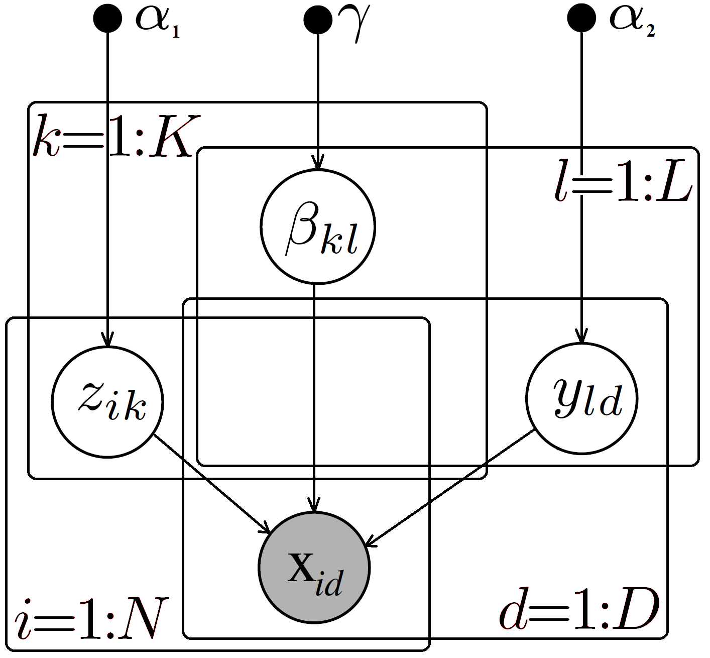
Figure 5: Graphical model for DMM with prior distributions. Filled circles are observed random variables and empty circles are hidden. Solid points denote fixed parameters of the model. Arrows indicate dependencies. Entities on a $N$-rectangle exist in $N$ different realizations.

Nonparametric Bayesian priors could, in principle, also be added to the flat RBAC model proposed above. However, as this model allows users to have multiple roles, the Dirichlet process prior is not applicable to $\mathbf{Z}$. Instead, the “Indian Buffet Process” [19] could be used as a prior. In our experiments, we compare with an algorithm that combines such a prior with a noisy-OR likelihood [39].

3.5 Noise

The goal of role mining is to infer the role structure underlying a given access control matrix. In this context, structure means permissions that are frequently assigned together and users that share the same set of permissions (not necessarily all their permissions). User-permission assignments that do not replicate over the users do not account for the structure. We call such exceptional assignments noise. A noisy bit can be an unusual permission or a missing assignment of a permission.

In this section we add an explicit noise process to the flat RBAC model. Let $x^{S}_{id}$ be a “structural” bit and let $x^{N}_{id}$ be a “noise” bit. While a structural bit is generated by the generation process of the user-permission assignments in the flat RBAC scenario given by Eq. (13), a noise bit is generated by a random coin flip with probability $r$:

$$p_{N}\left(x^{N}_{id}\left.\right|r\right)=r^{x^{N}_{id}}\left(1-r\right)^{1-x^{N}_{id}}\ .$$ (16)

Let $\xi^{S}_{id}$ be a binary variable indicating if the observed bit $x_{id}$ is a noise bit or a structure bit. Then the observed bit is

$$x_{id}=(1-\xi_{id})x^{S}_{id}+\xi_{id}x^{N}_{id}\ .$$ (17)

With the structure and noise distribution combined, the resulting probability of an observed $x_{id}$ is

$$p\!\left(x_{id}\!\left.\right|\mathcal{L}_{i},\boldsymbol{\beta},r,\mathbf{\xi}_{id}\right)\!=\!p_{N}\!\left(x_{id}\!\left.\right|r\!\right)^{\xi_{id}}p_{S}\!\left(x_{id}\!\left.\right|\mathcal{L}_{i},\boldsymbol{\beta}\right)^{1-\xi_{id}}\ .$$ (18)

In Appendix A.4 we marginalize out $\xi$ and obtain the final likelihood of this model.

$$p_{\text{MAC}}\left(\mathbf{X}\left.\right|\mathbf{Z},\boldsymbol{\beta},r,\epsilon\right) =\prod_{id}\left(\epsilon\cdot p_{N}\left(x_{id}\left.\right|r\right)+(1-\epsilon)\cdot p_{\text{flat}}\left(x_{id}\left.\right|\mathbf{Z},\boldsymbol{\beta}\right)\right)\ .$$ (19)

The generation process underlying this model is depicted in Figure 6. The advantage of an explicit noise process over threshold-based denoising methods [4] is the ability to automatically adapt to the data’s noise level. Another way to deal with noise is denoising in the continuous domain as a preprocessing step for a generic role mining method. Such an approach using SVD has shown good performance [31]. While this step is computationally inexpensive, it requires selecting a cutoff threshold.

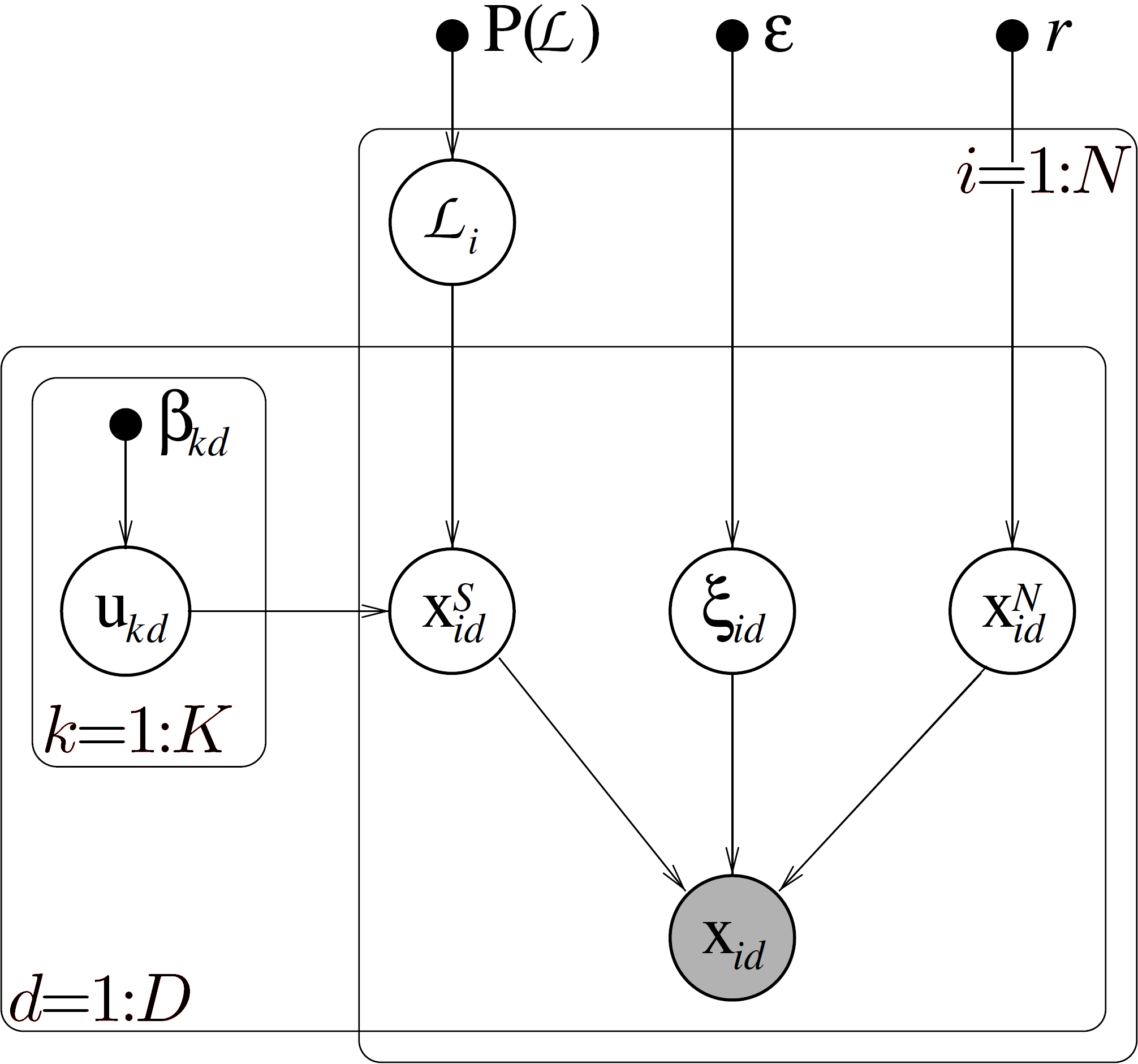
Figure 6: The generative model of Boolean MAC with mixture noise. $\mathcal{L}_{i}$ is the assignment set of user $i$, indicating which roles from $\mathbf{U}$ generated the user’s permissions. The bit $\xi_{id}$ selects whether the noise-free bit $x^{S}_{id}$ or the noise bit $x^{N}_{id}$ is observed. This model is an extension of the model in Fig. 3.

4 Learning the model parameters

In the last section we derived a class of probabilistic models. To apply these models to the role mining problem, we require algorithms that learn the model parameters from a given access control matrix. In this section we present two such learning algorithms. In particular, we use an annealed version of expectation-maximization (EM) for the models with a fixed number of parameters and Gibbs sampling for the non-parametric model variants.

4.1 Annealed EM

When applying the well-known EM algorithm to clustering problems, one alternates between updating the expected cluster assignments given the current centroids (E-step) and updating the centroids given the current assignments (M-step). In the case of the proposed model for multi-assignment clustering (MAC), the E-step computes the expected assignment $\gamma_{\mathcal{L},i}$ of a user $i$ to role set $\mathcal{L}$ for each role and each user:

$$\gamma_{\mathcal{L},i}=p(\mathcal{L}|\mathbf{X},\boldsymbol{\beta},\epsilon,r)^{1/T}\biggr{(}\sum_{\mathcal{L}=1}^{\left|\mathbb{L}\right|}p(\mathcal{L}|\mathbf{X},\boldsymbol{\beta},\epsilon,r)^{1/T}\biggr{)}^{-1}.$$ (20)

Here, we have introduced the computational temperature $T>0$. The case with $T=1$ reproduces the conventional E-step. The limit $T\rightarrow\infty$ yields the uniform distribution over all role sets and a low temperature $T\rightarrow 0$ makes the expectation of the assignments “crisp” (close to $0$ or $1$). The normalization ensures that the sum over all $\mathcal{L}\in\mathbb{L}$ equals $1$.

While iterating this modified E-step and the conventional M-step, we decrease the temperature starting from a value of the order of the negative log-likelihood costs. As a result, the local minima of the cost function are less apparent in the early stage of the optimization. In this way, lower minima can be identified than with conventional EM, although there is no guarantee of finding the global minimum. In addition to this robustness effect of the annealing scheme, we obtain the desired effect that, in the low-temperature regime of the optimization, the user-role assignments are pushed towards 0 and 1. As we are ultimately interested in binary user-role assignments, we benefit from forcing the model to make crisp decisions.

We provide the update equations of all model parameters used in the M-step in Appendix A.5. The rows of $\boldsymbol{\beta}$ are initialized with random rows of $1\!\!-\!\!\mathbf{X}$ and $(\epsilon,r)$ are initialized with $(0.1,0.5)$. The annealed optimization is stopped when the last user was assigned to a single role set with a probability exceeding $1-10^{-6}$.

4.2 Gibbs sampling

For nonparametric model variants as, for instance, the DDM with a Dirichlet process for the user-role assignments, we employ Gibbs sampling to learn the model parameters. Gibbs sampling iteratively samples the assignment of a user to one of the currently existing roles or to a new role while keeping the assignments of all other users fixed. This scheme explicitly exploits the exchangeability property of these models. This property states that the ordering in which new objects are randomly added to the clusters does not affect the overall distribution over all clusterings.

All terms involved in the sampling step are derived in Appendix A.3. The probability for assigning the current user to a particular role is given in Eq. (58). The Gibbs sampler alternates between iterating over all user-role assignments and over all permission-role assignments. It stops if the assignments do not change significantly over several consecutive iterations or if a predefined maximum number of alternations is reached. While running the sampler, the algorithm stores the state with the maximum a-posteriori probability and reports this state as the output. This book-keeping leads to worse scores than computing the estimated score by averaging over the entire chain of sampled RBAC configurations. However, this restriction to a single solution reflects the practical constraints of the role mining problem. Ultimately, the administrator must choose a single RBAC configuration.

5 Experiments

In this section we experimentally investigate the proposed models on both artificial and real-world datasets. We start by comparing MAC and DDM on datasets where we vary the noise level. Afterwards we compare MAC and DDM with other methods for Boolean matrix factorization on a collection of real-world datasets.

5.1 Comparison of MAC and DDM

MAC and DDM originate from the same core model. However, they differ in the following respects: First, DDM has one extra layer of roles. This additional layer, encoded in the assignment matrix $\mathbf{Y}$, creates a clustering of the permissions. Therefore, DDM has a two-level role hierarchy while MAC models flat RBAC. Second, DDM has additional constraints on its assignment matrices $\mathbf{Z}$ and $\mathbf{Y}$ dictating that the business roles must be disjoint in terms of their users and the technical roles must be disjoint in terms of their permissions. The assignments of business roles to technical roles $\mathbf{V}$ are unconstrained. MAC has no constraints at all. A user can have multiple roles and permissions can be assigned to multiple roles. The last difference between the two models are the prior assumptions on the model parameters. While MAC implicitly assumes uniform prior probabilities for its parameters, DDM makes explicit non-uniform assumptions encoded in the Beta priors and the Dirichlet priors.

To evaluate which of the two model variants is best suited to solve the role mining problem, we design the following experiment. We generate access control data in two different ways. One half of the datasets is generated according to the MAC model. We take a set of roles and randomly assign users to role combinations to create a user-permission assignment matrix. Then, we randomly select a defined fraction of matrix entries and replace them with the outcome of a fair coin flip. Some users in these datasets are generated by multiple roles. The second set of datasets is generated from the DDM probability distribution by repeatedly sampling business roles and technical roles from the Dirichlet process priors and randomly connecting them according to the Beta-Bernoulli probabilities.

On both kinds of data sets, we infer RBAC configurations with DDM and with MAC. In this way, the model assumptions always hold for one of the models while the other one operates in a model-mismatch situation. Moreover, data from DDM can have an arbitrary number of underlying roles. Therefore, MAC requires an additional model-order selection mechanism. Cross-validation with the generalization test described in Section 2.2 is employed as a quality measure.

We control the difficulty of the experiments by varying the noise level in the data. For each noise level, we sample 30 datasets from each model variant, each with 400 users and 50 permissions. On each dataset, we run each model 10 times and select the solution with the highest internal quality score, respectively. Finally, we evaluate the inferred roles based on their generalization error on a hold-out test set.

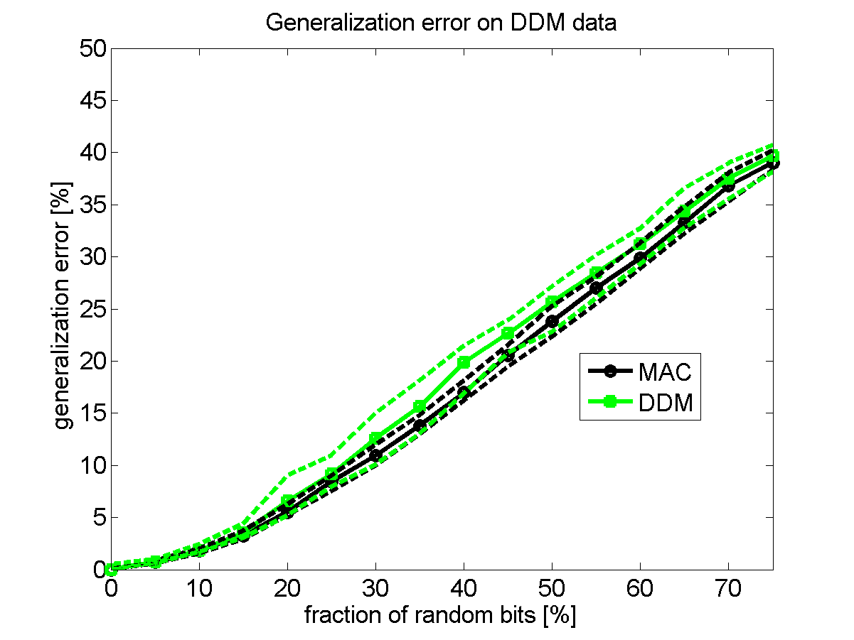
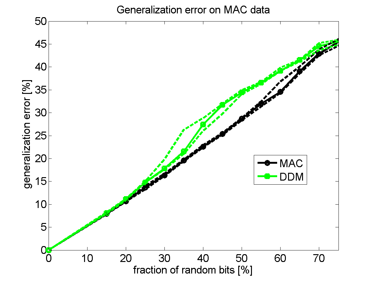
Figure 7: Comparison of the generalization error of MAC and DDM on data generated from a DDM role hierarchy and a flat RBAC configuration respectively.

Results

We report the median generalization error of the inferred matrix decompositions and the 25%/75%-percentiles in Figure 7. The left plot depicts the generalization error on DDM data and the right plot shows the error on MAC data.

We see that the overall trend of both models is similar for both types of data. The generalization error increases with increasing noise. There are two explanations for this behavior. First, the problem of estimating the structure of the data becomes increasingly difficult when increasing the noise level. Second, noisy bits are likely to be wrongly predicted, even when the data structure is learned well.

We also see that MAC and DDM generalize almost equally well on DMM data. MAC is even slightly better than DDM. In contrast, DMM achieves a worse generalization error than MAC on MAC data in the intermediate noise range. One would expect that each model generalizes best on data that is generated according to its assumptions. This behavior can be observed on MAC data. However, on DDM data MAC is as good as DDM. The reason is that for DMM data, the model assumptions of MAC are in fact not violated. Even though DMM has an extra layer of roles, this model instance is less complex than flat RBAC (which MAC models). One can see this by collapsing one DDM layer. For instance, define $\mathbf{u^{\prime}}:=\mathbf{v}\ast\mathbf{y}$. Then permissions can be assigned to multiple roles (because there are no constraints on the business-role to technical-role assignment $\mathbf{v}$). At the same time, $\mathbf{z}$ still provides a disjoint clustering of the users. In this flat RBAC configuration $(\mathbf{z},\mathbf{u^{\prime}})$ the roles overlap in terms of their permissions but not in terms of the users that are assigned to the roles. The same model structure arises in single-assignment clustering (SAC), a constrained variant of MAC, where users can have only one role. As a consequence, we can interpret DDM as a SAC model with prior probabilities on the model parameters. In contrast to MAC, SAC yields inferior parameter estimates as it must fit more model parameters for the same complexity of data. Hence, it has a larger generalization error.

In contrast to the structural difference between DDM and MAC, the differences in the optimization algorithm and in the Bayesian priors have only a minor influence on the results. It appears that MAC can compensate for a missing internal mechanism for finding the appropriate number of roles when an external validation step is provided. Also, the Gibbs sampling scheme and the deterministic annealing algorithm perform equally well on the DDM data. Given that the prior Beta distributions for the Bernoulli variables of the DDM provide no improvement over MAC, it seems unnecessary to extend MAC with such priors.

We experimentally confirmed that MAC is a more general model than DDM. We also found that the generalization error provides a good criterion for selecting the number of roles without making explicit prior assumptions on the distribution of this number. We therefore recommend using the MAC model for role mining with real-world datasets.

5.2 Noise

In this section we focus on erroneous user permission assignments. As explained in Section 2.1, the user-permission assignment matrix $U\!P\!A$ given as an input to the role mining problem contains exceptional or erroneous entries, which we refer to as noise. More precisely, we assume that a hidden noiseless assignment $U\!P\!A^{\prime}$ exists, but only $U\!P\!A$, a noisy version of it, is observable. By inferring a role structure $RC=(\mathbf{z},\mathbf{u})$ that supposedly underlies the input matrix $U\!P\!A$, our probabilistic models approximately reconstruct the noiseless matrix as $\mathbf{\hat{z}}\ast\mathbf{\hat{u}}$. In synthetic experiments, one can compare this reconstruction against the noise-free assignment $U\!P\!A^{\prime}$. We investigate two questions. First, how conservative are the RBAC configurations that our algorithms find, that is, how many new errors are introduced in the reconstruction? Second, does the probabilistic approach provide a measure of confidence for reconstructed user-permission assignments?

Figure 8 depicts error rates that provide answers to both questions. In Figure 8a we contrast the fraction of wrong reconstruction assignments that are new with the fraction of wrong input assignments that have not been discovered. To obtain these values, we ran experiments on input matrices created from the DDM with a fraction of randomized bits that varies from 5% to 75%. As can be seen, MAC’s ratio of newly introduced to repeated errors is constant for false negatives and false positives alike. DDM tends towards repeating old errors and introduces fewer new errors, while the sum of new and old errors is approximately the same as for MAC. The maximal sum of error rates is 8% false negatives and 7.5% false positives, which is small compared to the maximal fraction of random bits 75%.

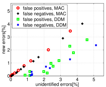
(a) New vs. old errors

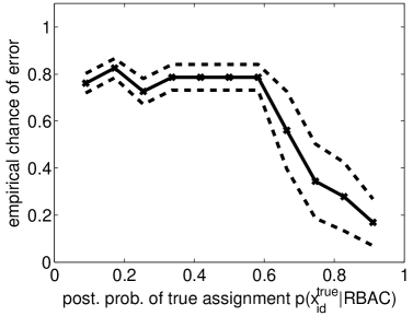
(b) Assignment Confidence

Figure 8: Error analysis. 8a: How many new errors are added to the assignment versus how many original errors were not identified? We distinguish false negatives from false positives. 8b: Trend of the empirical chance of creating a wrong assignment $x_{id}$ as a function of the posterior probability of the correct assignment given the learned RBAC configuration. It is apparent that the posterior provides a measure of confidence.

Figure 8b illustrates the empirical probability that a reconstructed user-permission assignment is wrong. The x-axis is the posterior probability of the true value $p(x_{id}^{\prime}|RC)$ of this assignment, i.e. the probability of reconstructing the assignment correctly as computed by the learned model. The plot convincingly illustrates that the posterior provides a measure of confidence. The stronger the model prefers a particular assignment (the closer the posterior is to 1), the less likely it is to introduce an error if one follows this preference. This model property means that, in addition to the RBAC configuration, our algorithms can output a confidence score for each resulting user-permission assignment. This uncertainty estimate could help practitioners when configuring RBAC using our methods.

5.3 Experiments on real-world data

In this section we compare MAC and DDM with other Boolean matrix factorization techniques on real-world datasets.

The first dataset LE-access comes from a Large Enterprise. It consists of the user-permission assignment matrix of $N=4900$ users and $D=1300$ permissions as well as business attributes for each user. In this section, we will ignore the business attributes but in Section 6 we will include them in a hybrid role mining process. The other datasets are six publicly available datasets from HP labs [9]. They come from different systems and scenarios. The dataset dominos is an access-control matrix from a Lotus Domino server, customer is the access-control matrix of an HP customer, americas small and emea are access-control configurations from Cisco firewalls, and firewall1 and firewall2 are created from policies of Checkpoint firewalls.

We compare several algorithms for Boolean matrix factorization on these datasets. In addition to DDM and MAC, there are two other probabilistic methods that have been developed in different contexts. Binary Independent Component Analysis (BICA) [22] learns binary vectors that can be combined to fit the data. These vectors, representing the roles in our setting, are orthogonal, that is, each permission can be assigned to only one role. In [39], an Indian buffet process has been combined with a noisy-OR likelihood to a nonparametric model that learns a Boolean matrix factorization. We call this model infinite noisy-OR (INO). The noisy-OR likelihood is closely related to the likelihood of MAC. The difference is that its noisy bits are always flipped to 1, whereas in MAC a noisy bit is a random variable that is 1 with probability $r$ and 0 otherwise. Similar to the Dirichlet process used in DDM, the Indian buffet process in INO is capable of learning the number of factors (here the number of roles). Another method that we compare with is a greedy combinatorial optimization of a matrix factorization cost function. This method, called Discrete Basis Problem solver (DBPS), was proposed in [28]. It finds a Boolean matrix decomposition that minimizes the distance between the input matrix and the Boolean matrix product of the two decomposition matrices. This distance weights false 1s differently compared to false 0s, with weighting factors that must be selected. The decomposition is successively created by computing a large set of candidate vectors (here candidate roles) and then greedily selecting one after the other such that in each step the distance function is minimized.

For each dataset, we randomly subsample a training set containing 80% of the users and a hold-out test set containing the remaining 20% users. All model parameters are trained on the training set and the generalization error is evaluated on the test set. We repeat this procedure five times with a different random partitioning of the training set and the test set.

We train the model parameters as follows. DDM and INO select the number of roles internally via the Dirichlet process and the Indian Buffet process, respectively. For MAC, BICA, and DBPS, we repeatedly split the training data into random subsets and compute the validation error. We then select the number of roles (and other parameters for BICA and DBPS, such as thresholds and weighting factors) with lowest validation error and train again on the entire training set using this number.

Table 1: Results on HP labs data

	customer			americas small
	10,021 users $\times$ 277 perms.			3,477 users $\times$ 1,587 perms.
	$k$	gen. error [%]	run-time [min]	$k$	gen. error [%]	run-time [min]
MAC	187	${{2.40\pm 0.03}}$	49	139	$1.03\pm 0.01$	80
DDM	4.6	$1.90\pm 0.01$	800	48.8	$1.00\pm 0.03$	2000
DBPS	178	$2.54\pm 0.05$	43	105	${1.00\pm 0.03}$	100
INO	20	$7.8\phantom{0}\pm 1.6\phantom{0}$	990	65.6	$1.05\pm 0.01$	300
BICA	82	$2.66\pm 0.02$	200	63	${1.00\pm 0.01}$	64
	firewall1			firewall2
	365 users $\times$ 709 perms.			325 users $\times$ 590 perms.
	$k$	gen. error [%]	run-time [min]	$k$	gen. error [%]	run-time [min]
MAC	49	${4.57\pm 0.01}$	10	10	${3.40\pm 0.00}$	1.8
DDM	24	$4.52\pm 0.01$	38	9.6	$11.28\pm 0.00$	5.4
DBPS	21	$13.6\phantom{0}\pm 3.1\phantom{0}$	5	4	$19.5\phantom{0}\pm 4.4\phantom{0}$	2
INO	38.2	$8.04\pm 0.00$	96	6.2	$11.15\pm 0.00$	14
BICA	18	$12.8\phantom{0}\pm 3.0\phantom{0}$	2.1	4	$19.9\phantom{0}\pm 4.5\phantom{0}$	0.9
	dominos			emea
	79 users $\times$ 231 perms.			35 users $\times$ 3,046 perms.
	$k$	gen. error [%]	run-time [min]	$k$	gen. error [%]	run-time [min]
MAC	7	$1.73\pm 0.00$	1.1	3	$8.7\phantom{0}\pm 1.2\phantom{0}$	0.7
DDM	6.4	$1.70\pm 0.01$	2.4	18.2	$8.4\phantom{0}\pm 0.1\phantom{0}$	143
DBPS	9	$2.3\phantom{0}\pm 0.5\phantom{0}$	0.2	8	${7.3\phantom{0}\pm 2.6\phantom{0}}$	1.1
INO	26	${1.7\phantom{0}\pm 0.1\phantom{0}}$	9.0	80.4	$10.1\phantom{0}\pm 2.4\phantom{0}$	204
BICA	3	$1.9\phantom{0}\pm 0.3\phantom{0}$	0.1	5	$8.6\phantom{0}\pm 2.8\phantom{0}$	1.0

Our experimental findings on the HP datasets are summarized in Table 9. We report the number of users and permissions and scores for each method: the number of roles discovered, the median generalization error and its average difference to the 25% and 75%-percentiles, and the the time required for one run. For americas small and emea the errors of all methods are within the percentiles. For customer, DDM generalizes best. For firewall1 and dominos, DDM and MAC perform equally well and lead the ranking, whereas for firewall2 DDM is inferior to MAC. While for all datasets MAC finds solutions with an error close to the solutions of the “winner”, DDM deviates largely from the best method in the case of firewall2.

All methods differ significantly in runtime with DBPS always being the fastest method. However, the run-times are difficult to compare for several reasons. First, all algorithms have been implemented by different authors in different programming languages. Second, they all use different stopping criteria. We manually selected these criteria such that each method achieves good results on training data, but it is impossible to tune them for a fair runtime comparison. Finally, all algorithms, except for INO and DDM, must be run several times to search for appropriate parameters. The runtimes reported in Table 1 account for one such run. To find the appropriate $k$ for MAC, DBPs, and BICA, we start with $k=2$ and increase $k$ until the generalization error significantly increases. The final value of $k$ given in Table 1 is thus indicative of the number of runs. For DBPs, we additionally tuned the parameters “threshold” and “bonuses” with a grid search over 25 candidate values.

The results on LE-access are graphically illustrated in Figure 9. The MAC model generalizes best. The two nonparametric Bayesian models DDM and INO have a similar performance. DBPS performs a bit worse and BICA has the highest generalization error. Apparently, on this dataset, the assumption of orthogonal roles does not hold.

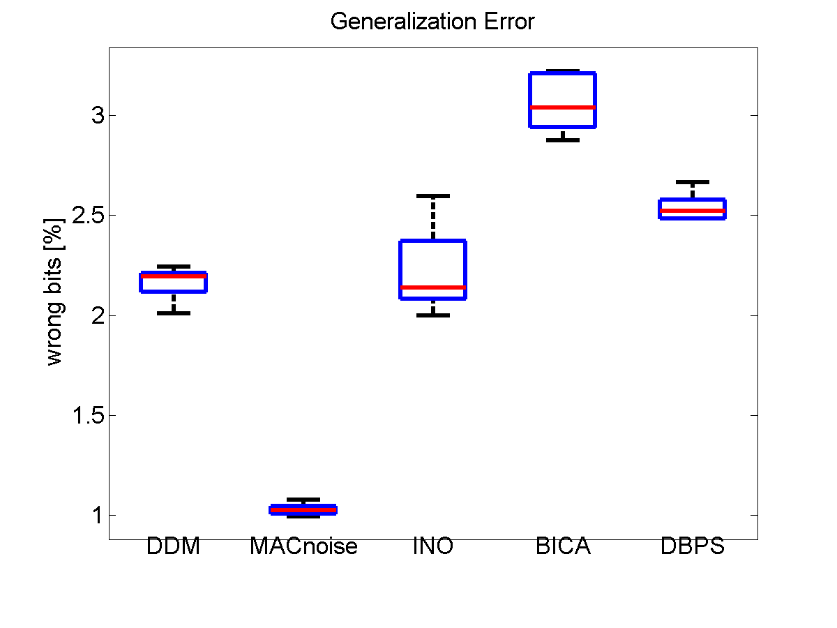
Figure 9: Generalization error on real-world data.

6 Hybrid role mining

Hybrid role mining accepts as input additional information on the attributes of the users or business processes. The goal, as defined by the inference role mining problem, remains unchanged: Find the RBAC configuration that most likely underlies the observed user-permission assignment. As this configuration is assumed to reflect the business properties and the security policies of the enterprise, we approach the hybrid role mining problem by jointly fitting an RBAC configuration to the user-permission assignment and to the business information given as additional input.

We account for this additional information by modifying the optimization problem for role mining. The original problem is to minimize the negative log-likelihood for the MAC model (19). The original cost function is

$$R^{(ll)} =\sum_{i,\mathcal{L}}z_{i\mathcal{L}}R_{i,\mathcal{L}}^{(ll)}\ ,\ \ z_{i\mathcal{L}}\in\{0,1\},\ \ \forall i:\sum_{\mathcal{L}}z_{i\mathcal{L}}=1\,.$$ (21)

Here we used the assignments $z_{i\mathcal{L}}$ from user $i$ to the set of roles $\mathcal{L}$. With these assignments and with the assignments $z_{\mathcal{L}k}$ from role sets to roles, a user is assigned the roles, which are contained in the role set that he is assigned to ($z_{ik}=\sum_{\mathcal{L}}z_{i\mathcal{L}}z_{\mathcal{L}k}$). The individual costs of assigning a user $i$ to the set of roles $\mathcal{L}$ is

$$R_{i,\mathcal{L}}^{(ll)} =-\log\left(\prod_{d}p_{M}\left(x_{id}\left.\right|\mathcal{L},\mathbf{\beta},r,\epsilon\right)\right)\,.$$ (22)

We now add an additional term to this negative log-likelihood cost function to define an objective function for hybrid role mining. We use a linear combination of the likelihood costs Eq. (21) and a term $R^{(S)}$ that accounts for business information costs:

$$R:=R^{(ll)}\!/D+\lambda R^{(S)}\,,$$ (23)

where $\lambda\geq 0$ weights the influence of the business information. The term $1/D$ makes the likelihood costs independent of the number of permissions $D$.

Role mining without business information is a special case of Eq (23), where $\lambda=0$, whereby role mining optimizes the model parameters with respect to Eq. (21). This problem has a huge solution space, spanned by the model parameters, with many local minima. By incorporating business information into this optimization problem ($\lambda>0$), we introduce a bias toward minima that correspond to the business attributes used as additional input.

We consider an RBAC configuration to be meaningful if employees satisfying identical business predicates (that is, having the same business attributes) are also assigned to similar (ideally identical) sets of roles. To account for this, we propose an objective function $R^{(S)}$ that computes the similarity of the role assignments of all pairs of users with the same business attributes. $R^{(S)}$ compares all pairs of users $(i,i^{\prime})$ having the business attribute $s$ with respect to their role assignments $(z_{i\cdot}$, $z_{i^{\prime}\cdot})$. Let $w_{is}\!\in\!\{0,1\}$ encode whether user $i$ has business attribute $s$ ($w_{is}=1$) or not ($w_{is}=0$). Then the cost of a user-role assignment matrix $\mathbf{Z}$ is

$$R^{(S)}\!\! = \!\!\frac{1}{N}\sum_{s}\sum_{i,i^{\prime}}w_{is}w_{i^{\prime}s}\sum_{k}z_{i^{\prime}k}\left(1-2z_{i^{\prime}k}z_{ik}\right).$$ (24)

$N$ is the total number of users and $k\in\{1,\ldots,K\}$ is the role index. Each user has a single business attribute $s$, that is $\sum_{s}w_{is}=1$, but can be assigned to multiple roles, $1\leq\sum_{k}z_{ik}\leq K$. The term $\sum_{k}z_{i^{\prime}k}\left(1-2z_{i^{\prime}k}z_{ik}\right)$ in Eq. (24) computes the agreement between the binary assignment vectors $(z_{i\cdot},z_{i^{\prime}\cdot})$ for all pairs of users $(i,i^{\prime})$ having the same attribute $s$ (which is the case iff $w_{is}w_{i^{\prime}s}\!=\!1$). The subterm $1-2z_{i^{\prime}k}z_{ik}$ switches the sign of a single term such that agreements ($z_{ik}z_{i^{\prime}k}=1$) are rewarded and differences ($z_{ik}z_{i^{\prime}k}=0$) are penalized. An alternative to Eq. (24) would be to compute the Hamming distance between the two assignment vectors. However, this has the drawback of penalizing pairs with differently sized role sets. We have chosen the dissimilarity function in Eq. (24) to avoid a bias towards equally sized role sets.

Note that our objective function conceptually differs from those proposed in [3, 29, 30, 40]. While we minimize the role dispersion of users with the same attributes, their objective is to minimize measures of attribute dispersion [40] of users with the same roles. We see two advantages of our cost function. First, it enables multiple groups of users with different attributes to share roles, such as users of all organizational units getting a “standard role”. Second, it is easier to add new users in our framework as usually the attributes of new users are given whereas the roles are not.

Optimization

We now demonstrate how to optimize the new cost function for hybrid role mining using the deterministic annealing framework presented in Section 4. Specifically, we convert the term $R^{(S)}$ into a form that enables us to conveniently compute the responsibilities $\gamma_{i\mathcal{L}}$ in the E-step.

The responsibility $\gamma_{i\mathcal{L}}$ of the assignment-set $\mathcal{L}$ for data item $i$ is given by

$$\gamma_{i\mathcal{L}}:=\frac{\exp\left(-R_{i\mathcal{L}}/T\right)}{\sum_{\mathcal{L}^{\prime}\in\mathbb{L}}\exp\left(-R_{i\mathcal{L}^{\prime}}/T\right)}\ .$$ (25)

In Eq. (20), the individual cost terms were $R_{i\mathcal{L}}=-\log\left(p(\mathbf{x_{\ast i}}|\mathcal{L}_{i},\boldsymbol{\beta},\epsilon,r)\right)$. Now the full costs are extended with $R^{(S)}$. To compute Eq. (25), we shall rewrite $R^{(S)}$ as a sum over the individual contributions of the users.

Let $N_{sk}:=\sum_{i}z_{ik}w_{is}$ be the number of users that have the business attribute $s$ and are assigned to role $k$, and let $s_{i}$ be the attribute of user $i$. We first simplify and reorganize Eq. (24) using these auxiliary variables

$$R^{(S)} =\frac{1}{N}\sum_{s}\sum_{i}w_{is}\sum_{k}\left(N_{sk}-2z_{ik}N_{sk}\right)$$

$$=\frac{1}{N}\sum_{i}\sum_{k}\left(N_{s_{i}k}-2z_{ik}N_{s_{i}k}\right)$$

$$=\sum_{i,k}\left(1-z_{ik}\right)\frac{N_{s_{i}k}}{N}-\sum_{i,k}z_{ik}\frac{N_{s_{i}k}}{N}\ .$$ (26)

In this formulation, it becomes apparent that user $i$ with attribute $s_{i}$ should be assigned to the role $k$ ($z_{ik}=1$) if many users have attribute $s_{i}$ and role $k$.

Finally, we decompose the costs into individual contributions of users and role sets. We use the notion of user-to-role set assignments $z_{i\mathcal{L}}$ to substitute the user-role assignments by $z_{ik}=\sum_{\mathcal{L}}z_{i\mathcal{L}}z_{\mathcal{L}k}$:

$$R^{(S)} =\sum_{i,k}\left(\left(1-\sum_{\mathcal{L}}z_{i\mathcal{L}}z_{\mathcal{L}k}\right)\frac{N_{s_{i}k}}{N}-\sum_{\mathcal{L}}z_{i\mathcal{L}}z_{\mathcal{L}k}\frac{N_{s_{i}k}}{N}\right)$$

$$=\sum_{i,\mathcal{L}}z_{i\mathcal{L}}\left(\sum_{k\notin\mathcal{L}}\frac{N_{s_{i}k}}{N}-\sum_{k\in\mathcal{L}}\frac{N_{s_{i}k}}{N}\right)\ \ =\sum_{i,\mathcal{L}}z_{i\mathcal{L}}R_{i,\mathcal{L}}^{(S)}\ \ .$$ (27)

In this form we can directly compare the business cost function with the likelihood costs given by Eq. (22). We can therefore easily compute the expectation in the E-step by substituting the costs in Eq. ( 25) with $R_{i\mathcal{L}}=R_{i,\mathcal{L}}^{(ll)}+R_{i,\mathcal{L}}^{(S)}$.

In the iterative update procedure of the deterministic annealing scheme, one faces a computational problem arising from a recursion. The optimal assignments $z_{i\mathcal{L}}$ depend on the $N_{s_{i}k}$, which are, in turn, computed from the $z_{i\mathcal{L}}$ themselves. To make this computation at step $t$ of our algorithm feasible, we use the expected assignments $\gamma_{i\mathcal{L}}^{(t-1)}:=\mathbb{E}\left[z_{i\mathcal{L}}^{(t-1)}\right]$ of the previous step instead of the Boolean $z_{i\mathcal{L}}^{(t)}$ to approximate $N_{s_{i}k}^{(t)}$ by its current expectation with respect to the Gibbs distribution:

$$N_{s_{i}k}^{(t)}\approx\mathbb{E}\left[N_{s_{i}k}^{(t-1)}\right]=\sum_{\mathcal{L}}z_{\mathcal{L}k}\sum_{i^{\prime}}w_{i^{\prime}s_{i}}\gamma_{i^{\prime}\mathcal{L}}^{(t-1)}\,.$$ (28)

We do not have a proof of convergence for this algorithm. However we observe that when running it multiple times with random initializations, it repeatedly finds the same solution with low costs in terms of business information and model likelihood.

6.1 Selecting relevant user attributes

An important step for hybrid role mining is selecting of the set of user attributes used as input for the optimizer. User attributes that do not provide information about the users’ permissions should not be used for hybrid role mining. In fact, requiring that the roles group together users with irrelevant attributes can result in inferred RBAC configurations that are worse than those inferred without using the attributes.

To select appropriate user attributes, we propose an information theoretic measure of relevance. Let the random variable $X_{d}\in\{0,1\}$ be the assignment of permission $d$ to a generic user. $S$ is the random variable that corresponds to the business attribute of a generic user (e.g. “job code”) and let $s$ be one of the actual values that $S$ can take (e.g. “accountant”). Let $p(x_{d}):=1/N\cdot\sum_{i}x_{id}$ be the empirical probability of $d$ being assigned to an unspecified user, and let $p(x_{d}|S=s):=1/N\cdot\sum_{i}x_{id}w_{is}$ be the empirical probability of $d$ being assigned to a user with business attribute $s$. With these quantities, we define the binary entropy, the conditional entropy, and the mutual information as:

$$h(X_{d}) := -\!\!\sum_{x_{d}\in\left\{0,1\right\}}\!\!p(x_{d})\log_{2}\left(p(x_{d})\right)\ ,$$ (29)

$$h(X_{d}|S) := \!-\!\!\sum_{s\in S}p(s)\!\!\!\!\!\sum_{x_{d}\in\left\{0,1\right\}}\!\!\!\!\!p(x_{d}|S=s)\log_{2}\left(p(x_{d}|S=s)\right)\ ,$$ (30)

$$I(X_{d};S) := h(X_{d})-h(X_{d}|S)\ .$$ (31)

The entropy $h(X_{d})$ quantifies the uncertainty about whether a user is assigned permission $d$. The conditional entropy $h(X_{d}|S)$ is the uncertainty for a user whose business attribute $S$ is known. The mutual information $I(X_{d};S)$ is the absolute increment of information about the user-permission assignment gained by knowledge of $S$. This number indicates how relevant the attribute $S$ is for the assignment of permissions. There is one pitfall, though. If one compares this score on different permissions $d$ with different entropies $h(X_{d})$, then low-entropic permissions will have a smaller score simply because there is little entropy to reduce. We therefore compute the relative mutual information ([6], p. 45) as a measure of relevance:

$$\rho_{d}(S):=I(X_{d};S)/h(X_{d})=1-h(X_{d}|S)/h(X_{d})\,.$$ (32)

We use the convention $0/0:=1$ for the case where $h(X_{d})=0$ (then $I(X_{d};S)$ will also be $0$). This number can be interpreted as the fraction of all bits in $X_{d}$ that are shared with $S$. Alternatively, $\rho_{d}(S)$ can be read as the fraction of missing information about permission $d$ that is removed by the knowledge of $S$.

Limit of few observations per business attribute

One should take care to use sufficiently many observations when estimating the relevance $\rho_{d}(S)$ of a business attribute $S$. With too few observations, this measure is biased towards high relevance. Imagine the problem of estimating the entropy of a fair coin based on only one observation (being heads without loss of generality). Naïvely computing the empirical probability of heads to be $1$ provides an entropy of $0$, which differs considerably from the true entropy of a fair coin which is $1$ bit. The same effect occurs when one computes the permission entropy conditioned on an irrelevant attribute where only one observation per attribute value is available. In [31], for instance, the last name of a user was found to be highly relevant! A practical solution is to compute $\rho_{d}(S)$ with only those values of $S$ where sufficiently many observations are available. For instance, if more than 10 users have the feature $s$=“Smith”, the empirical probability $p(x_{d}|S=s)$ will give a good estimate of $h(x_{d}|S=s)$. In our experiments, we neglected all attribute values with less than 10 observations.

Figure 10: Distribution of the measure of relevance Eq. (32), the mutual information weighted with inverse permission entropy.

We apply the proposed relevance measure to the two different user attributes of the LE-access dataset, the job code (JC) and the organizational unit (OU) of a user. The first attribute is each user’s so-called job code, which is a number that indexes the kind of contract that the user has. We initially believed that this attribute would be highly relevant for each user’s permission as it is indicative of the user’s business tasks. We compute the relevance of these two attributes for each permission. The results are depicted in Figure 10. In these histograms, we count the number of permissions for which the respective user attribute has the given relevance score. As can be seen, the average reduction in entropy is much higher for the OU (87.8%) than for JC (49.7%). This result means that knowledge of the OU almost determines most of the permissions of the users while the JC provides relatively little information about the permissions. We therefore only use OU in our role mining experiment.

6.2 Results for hybrid role mining

We run experiments on the LE-access dataset. This time, we use the adapted E-step as derived in Section 6 with the organizational unit (OU) of the user as the business attribute $S$. Again, we randomly split the data into a training set and a test set, learn the roles on the training set, and then compute the generalization error on the test set. This time, we fix the number of roles to $k=30$ and only study the influence of the business attributes on the result by varying the mixing parameter $\lambda$.

To evaluate how well the resulting role configuration corresponds to the business attributes of the user, we compute the average conditional role entropy:

$$h(\mathcal{L}|S):=\!-\frac{1}{N}\sum_{i=1}^{N}\sum_{\mathcal{L}}p(z_{i\mathcal{L}}|S=s_{i})\log_{2}\left(p(z_{i\mathcal{L}}|S=s_{i})\right)\,.$$ (33)

This number indicates how hard it is to guess the role assignments $z_{i\mathcal{L}}$ of a user $i$ given his organizational unit $s_{i}$. For a good RBAC configuration this entropy is small, meaning that the knowledge of the organizational unit suffices to determine the set of roles that the user has. If the RBAC configuration does not correspond to the organizational units at all, then knowledge of this attribute does not provide information about a user’s roles and, as a result, the role entropy is high. The advantage of the conditional role entropy over other measures of dispersion such as, for instance, nominal variance [8] or attribute-spread [3], is that it directly resembles the task of an administrator who must assign roles to new users. When deciding which roles should be assigned to a user given his business attributes, there should be as little uncertainty as possible. For the same reason, we select relevant business information by relative mutual information instead of heuristic scores such as “mineability” [5].

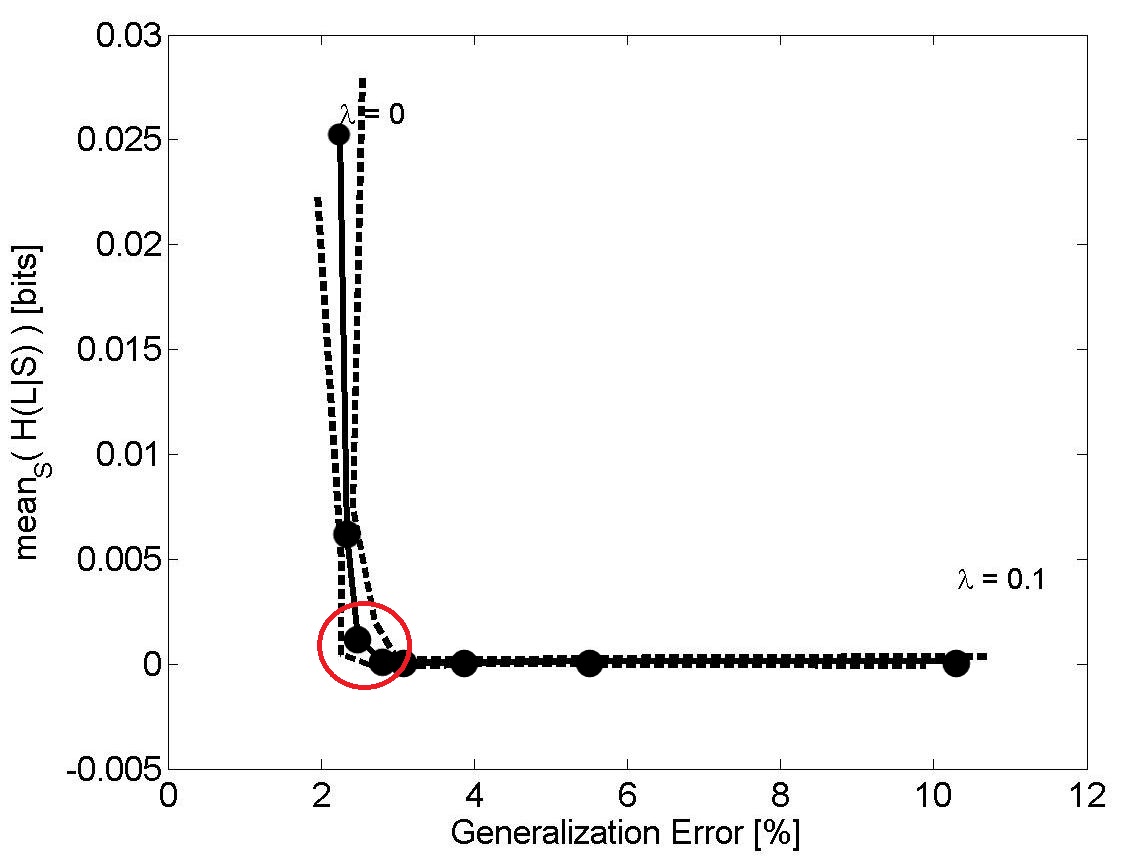
Figure 11: Generalization error versus conditional role entropy for the experiment using organization units. The dashed lines represent the standard deviation over ten repeated experiments.

We depict the results in Figure 11. We plot the role entropy against the generalization error. Each point on this line is the median result over ten experiments with different random splits in the training set and the test set. Each point is computed with a different mixing parameter $\lambda$. The plot demonstrates that by increasing the influence of the organizational unit, the role entropy decreases while the generalization error increases. This reduction means that hybrid role mining with this attribute requires a trade-off. Fortunately, most reduction in role entropy can be achieved without significantly increasing the generalization error. When further increasing $\lambda$, the generalization error increases without significantly improving role entropy. This insensitivity indicates a Pareto-optimum (marked with a circle in Figure 11), which defines the influence that one should give to user attributes in hybrid role mining. Note that, we are able to find this point (to produce Figure 11) without knowledge of the true roles.

7 Related work

Shortly after the development of RBAC [12], researchers and practitioners alike recognized the importance of methods for role engineering, see for instance [7]. As explained in the introduction, these methods can be classified as being either top-down or bottom-up. Top-down methods use process descriptions, the organizational structure of the domain, or features of the employees as given by the Human Resources Department of an enterprise, to create roles. [32], for instance, present a scenario-driven approach where a scenario’s requirements are analyzed according to its associated tasks. Permissions are then granted that enable the task to be completed. In [10], a work flow is proposed to manually engineer roles by analyzing business processes. Today, all pure top-down approaches are manually carried out. Bottom-up role methods have the advantage that they can be partially or fully automated by role mining algorithms, thereby relieving administrators from this time-consuming and error-prone task.

The first bottom-up role mining algorithm was proposed in [24] and coined role mining. Since then, a number of different bottom-up approaches have been presented. For instance, the algorithm of [33] merges sets of permissions to construct a tree of candidate roles. Afterwards, it selects the final roles from this tree such that, at every step, the permissions of a maximum number of users are covered. Subsequent role mining algorithms usually followed a similar structure: they first construct a set of candidate roles and afterwards greedily select roles from this set [37, 41, 2]. These algorithms differ from each other with respect to the proposal creation step or the cost function used to select roles. Vaidya et al. formally defined the role mining problem and variants in [35] and [36] and investigated the complexity of these problems. The problem definitions proposed in these two papers differ from our role inference problem in that either the number of roles or the number of residuals tolerated when fitting the RBAC configuration is given as input. Moreover, these definitions aim at a high compression rate, while role inference aims at discovering the latent roles that underlie the data.

The results presented in this paper build upon our prior work. In [14], we analyze the different definitions of role mining and define the role inference problem. In [13], we derive DDM from the deterministic permission assignment rule in RBAC. In [34], we propose the MAC model, which we explore further in [17], adding different noise processes. [15] focuses on determining the number of roles for role mining in particular, and selecting the number of patterns in unsupervised learning in general. Finally, in [16] we propose the hybrid role mining algorithm that we revisit in Section 6.

In this paper, we extend and generalize our prior work. In particular, we draw connections between all these concepts and approaches. We thereby generalize them within one consistent framework that covers i) the definition of role mining, ii) the approach to solve it, and iii) methods to evaluate solutions. While in [14] we motivate the role inference problem by analyzing the real-world requirements of RBAC, here we take a more direct approach. We identify the input that is usually available in realistic scenarios and directly derive the role inference problem from these assumptions. Moreover, we subsume the models of our prior work, DDM and MAC, within one core model. In this way, we analyze the relationships between them and highlight the influence of noise processes, role hierarchies, and constraints on role assignments. This theoretical comparison of the models is supplemented by an experimental comparison of DDM, MAC, and other models and algorithms. In addition, we provide a sound measure of confidence for user permission assignments and investigate how conservatively the proposed methods modify noisy assignments. We also show that DDM is structurally equivalent to a MAC model constrained to every user only having one role. Finally, our paper contains the first experimental comparison of DDM and MAC on both synthetic and real-world data.

8 Conclusion

We put forth that, in contrast to conventional approaches, role mining should be approached as a prediction problem, not as a compression problem. We proposed an alternative, the role inference problem, with the goal of finding the RBAC configuration that most likely underlies a given access control matrix. This problem definition includes the hybrid role mining scenario when additional information about the users or the system is available. To solve the role inference problem, we derived a class of probabilistic models and analyzed several variants. On real-world access control matrices, our models demonstrate robust generalization ability while other methods are rather fragile and their generalization ability depends on the particular data analyzed.

Acknowledgement

We thank Andreas Streich for discussions and the collaboration on hybrid role mining.

Appendix A Appendix

A.1 Marginalization

We convert the deterministic formula Eq. (6) into a probabilistic version by marginalizing out the latent variables $\mathbf{u}_{kd}$ from the joint distribution for $\mathbf{u}_{kd}$ and $x_{id}$. The joint distribution is

$$p(x_{id}=0,\mathbf{u}_{\ast d}|\boldsymbol{\beta}_{\ast d},\mathbf{z}_{i\ast})=p(x_{id}=0|\mathbf{u}_{\ast d},\mathbf{z}_{i\ast})\prod_{k}p(u_{kd}|\beta_{kd})\ .$$ (34)

As a single bit $x_{id}$ depends on the outcome of a full bitvector $\mathbf{u}_{\ast d}$ of length $K$, one must marginalize over all realizations of such bit-vectors.

Let $\Omega$ be the set of all possible binary vectors $\mathbf{u}_{\ast d}$. Then the likelihood for $x_{id}=0$ is

$$p(x_{id} =0|\boldsymbol{\beta}_{\ast d},\mathbf{z}_{i\ast})$$ (35)

$$=\sum_{\mathbf{u}_{\ast d}\in\Omega}p(x_{id}=0,\mathbf{u}_{\ast d}|\boldsymbol{\beta}_{\ast d},\mathbf{z}_{i\ast})$$ (36)

$$=\sum_{\mathbf{u}_{\ast d}\in\Omega}p(x_{id}=0|\mathbf{u}_{\ast d},\mathbf{z}_{i\ast})\prod_{k}p(u_{kd}|\beta_{kd})$$ (37)

$$=\sum_{\mathbf{u}_{\ast d}\in\Omega}\prod_{k}\left(1-u_{kd}\right)^{z_{ik}}\left(\beta_{kd}^{1-u_{kd}}(1-\beta_{kd})^{u_{kd}}\right)$$ (38)

$$=\sum_{\mathbf{u}_{\ast d}\in\Omega}\left(\prod_{k:z_{ik}=1}\left(1-u_{kd}\right)^{z_{ik}}\beta_{kd}^{1-u_{kd}}(1-\beta_{kd})^{u_{kd}}\right)\left(\prod_{k:z_{ik}=0}\beta_{kd}^{1-u_{kd}}(1-\beta_{kd})^{u_{kd}}\right)\,.$$ (39)

In the step from (38) to (39) we substituted the individual probabilities with their definitions Eq. (3) and Eq. (6). In the last step, we separated the bit-vectors $\mathbf{u}_{\ast d}$ into the two cases where $z_{ik}=1$ and $z_{ik}=0$. The first case cancels all contributions of the sum where $z_{ik}=u_{kd}=1$ and for $z_{ik}=1,u_{kd}=0$ only the factor $\beta_{kd}$ remains. Therefore, it is convenient to introduce a modified set of bit-vectors $\Omega^{\prime}\!=\!\left\{\mathbf{u}_{\ast d}\in\Omega\;|u_{kd}=0\ \text{, for all }k\text{ with }z_{ik}=1\right\}\subset\Omega$, i.e., the entries of $u_{kd}$ that are relevant for object $i$ are fixed to $0$. The likelihood then takes the following compact form

$$p(x_{id}\!=\!0|\boldsymbol{\beta}_{\ast d},\mathbf{z}_{i\ast})\!=\!\!\!\sum_{\mathbf{u}_{\ast d}^{\prime}\in\Omega^{\prime}}\!\left\{\!\!\left(\prod_{k:z_{ik}=1}\!\!\!\beta_{kd}\!\!\right)\!\left(\prod_{k:z_{ik}=0}\!\!\!\beta_{kd}^{1-u_{kd}^{\prime}}(1-\beta_{kd})^{u_{kd}^{\prime}}\!\right)\!\!\right\}\!\,.$$ (40)

The sum in Eq. (40) has $\left|\Omega^{\prime}\right|$ terms. Let us pick a particular $k^{\prime\prime}$ with $z_{ik^{\prime\prime}}=0$. Half of the vectors in $\Omega^{\prime}$ have $u_{k^{\prime\prime}j}=1$ and the other half have $u_{k^{\prime\prime}j}=0$, whereas the remaining bits $k\neq k^{\prime\prime}$ are equal in both halves. We can therefore factor out the terms where bitvectors differ only at position $k^{\prime\prime}$ in Eq. (40). This reduces the number of terms in the sum by a factor of two, whereby the sum now ranges over the modified set $\Omega^{\prime\prime}\subset\Omega^{\prime}$, where all bits are varied except for $k^{\prime\prime}$.

In the following steps, we recursively factor out such terms. This successively interchanges the sum and the product in Eq. (40) and makes it easy to see, in Eq. (47), that all contributions with $z_{ik}=0$ sum up to $1$.

$$p(x_{id}=0|\beta_{\ast d},\mathbf{z}_{i\ast})$$ (41)

$$=\beta_{k^{\prime\prime}j}^{z_{ik^{\prime\prime}}}\underbrace{\left((1-\beta_{k^{\prime\prime}j})+\beta_{k^{\prime\prime}j}\right)}_{=1\;\forall k^{\prime\prime}}\sum_{\mathbf{u^{\prime\prime}}_{\ast d}\in\Omega^{\prime\prime}}\;\Biggl{(}\prod_{{\begin{array}[]{cl}k:z_{ik}=1\\ k\neq k^{\prime\prime}\end{array}}}\beta_{kd}^{z_{ik}}\Biggr{)}\Biggl{(}\prod_{{\begin{array}[]{cl}k:z_{ik}=0\\ k\neq k^{\prime\prime}\end{array}}}\beta_{kd}^{1-u^{\prime\prime}_{kd}}(1-\beta_{kd})^{u^{\prime\prime}_{kd}}\Biggr{)}$$ (46)

$$=\left(\prod_{k}\beta_{kd}^{z_{ik}}\right)\Biggl{(}\prod_{k:z_{ik}=0}\;\underbrace{\sum_{u^{\prime}_{kd}\in\left\{0,1\right\}}\beta_{kd}^{1-u^{\prime}_{kd}}(1-\beta_{kd})^{u^{\prime}_{kd}}}_{=1\;\forall k}\Biggr{)}=\prod_{k}\beta_{kd}^{z_{ik}}$$ (47)

A.2 Hierarchies

We compute the probability that a user is not assigned to a permission in a two-level role hierarchy given the probabilities of independent role hierarchy parameters. We start from Eq. (9).

$$\hbox to0.0pt{\hss$p$}\left(\overline{x_{id}}\ {|\mathbf{z}_{i\ast}^{+},\mathbf{y}_{\ast d}^{+},V^{+}}\right) =p\left(\overline{\bigvee_{k=1}^{K}\left[z_{ik}\wedge\left(\bigvee_{l=1}^{L}v_{kl}\wedge y_{ld}\right)\right]}\ {|\mathbf{z}_{i\ast}^{+},\mathbf{y}_{\ast d}^{+},V^{+}}\right)\begin{array}[]{clrr}1\!\!\leq\!\!k\!\!\leq\!\!K\!\!\\ \!\!1\!\!\leq\!\!l\!\!\leq\!\!L\end{array}$$ (50)

$$=\prod_{k}p\biggl{(}\overline{z_{ik}\wedge\underbrace{\biggl{(}\bigvee_{l}v_{kl}\wedge y_{ld}\biggr{)}}_{=:u_{kd}}}{\ |\mathbf{z}_{i\ast}^{+},\mathbf{y}_{\ast d}^{+},\mathbf{v}_{k\ast}^{+}}\biggr{)}$$ (51)

$$=\prod_{k}\!\Bigl{(}\!\underbrace{p\!\left(\overline{z_{ik}}\!\wedge\!u_{kd}{|z_{ik}^{+},\mathbf{y}_{\ast d}^{+},\mathbf{v}_{k\ast}^{+}}\right)\!+\!p\!\left(\overline{z_{ik}}\!\wedge\!\overline{u_{kd}}{|z_{ik}^{+},\mathbf{y}_{\ast d}^{+},\mathbf{v}_{k\ast}^{+}}\right)}_{=p\left(\overline{z_{ik}}{|z_{ik}^{+}}\right){=1-z_{ik}^{+}}}\!+\!p\!\left(z_{ik}\!\wedge\!\overline{u_{kd}}{|z_{ik}^{+},\mathbf{y}_{\ast d}^{+},\mathbf{v}_{k\ast}^{+}}\right)\!\Bigr{)}$$ (52)

$$={\prod_{k}\left(1-z_{ik}^{+}+z_{ik}^{+}\ p(\overline{u_{kd}}{|\mathbf{y}_{\ast d}^{+},\mathbf{v}_{k\ast}^{+}})\right)}$$ (53)

Note that in the step from (51) to (52), the correct probability is only obtained when summing over the probabilities of exclusive events (in particular: $\overline{a\wedge b}=\overline{a}\vee\overline{b}$ but $p\left(\overline{a\wedge b}\right)\neq p\left(\overline{a}\right)+p\left(\overline{b}\right)$). Given the generation $u_{kd}=\bigvee_{l}v_{kl}\wedge y_{ld}.$, we have that

$$p(\overline{u_{kd}}{|\mathbf{y}_{\ast d}^{+},\mathbf{v}_{k\ast}^{+}}) = \prod_{l}p\left(\overline{v_{kl}\wedge y_{ld}}{|y_{ld}^{+},v_{kl}^{+}}\right)=\prod_{l}\left[p(\overline{y_{ld}}{|y_{ld}^{+}})+p(y_{ld}{|y_{ld}^{+}})p(\overline{v_{kl}}{|v_{kl}^{+}})\right]\,.$$ (54)

Substituting this into Eq. (53) yields

$$\hbox to0.0pt{\hss$p$}\left(\overline{x_{id}}\ {|\mathbf{z}_{i\ast}^{+},\mathbf{y}_{\ast d}^{+},V^{+}}\right)={\prod_{k}\left(1-z_{ik}^{+}+z_{ik}^{+}\ \prod_{l}\left(1-y_{ld}^{+})+y_{ld}^{+}(1-v_{kl}^{+})\right)\right)}\,.$$ (55)

A.3 Gibbs Sampling Algorithm for DDM

Here, we derive all necessary distributions for the Gibbs sampling algorithm for DDM in Section 4.2. We start by collecting all distributions that define the model. The data likelihood of the model is

$$p\left(\mathbf{X}|\mathbf{Z},\mathbf{Y},\boldsymbol{\beta}\right) =\prod_{k,l}\left(1-\beta_{kl}\right)^{n^{(1)}_{kl}}\beta_{kl}^{n^{(0)}_{kl}}\,,$$ (56)

with the counters $n^{(1)}_{kl}=\sum_{\genfrac{}{}{0.0pt}{}{i:z_{ik}=1,}{j:y_{lj}=1}}\mathbf{I}_{\left\{x_{ij}=1\right\}}$ and $n^{(0)}_{kl}=\sum_{\genfrac{}{}{0.0pt}{}{i:z_{ik}=1,}{j:y_{lj}=1}}\mathbf{I}_{\left\{x_{ij}=0\right\}}\ .$ The parameters $\beta_{kl}$ are random variables themselves. They follow the Beta distribution

$$P_{b}\left(\beta_{kl};\gamma,\gamma\right) =\frac{\Gamma(2\gamma)}{2\Gamma(\gamma)}\left(\beta_{kl}(1-\beta_{kl})\right)^{\gamma-1}=B(\gamma,\gamma)^{-1}\left(\beta_{kl}(1-\beta_{kl})\right)^{\gamma-1}\ .$$ (57)

Here $B(.,.)$ is the beta function, also known as “Euler integral of the first kind”.

In each step, one must sample new assignments of user $i^{\prime}$ to roles from the distribution

$$p\left(z_{i^{\prime}k}\!=\!1|\mathbf{X},\mathbf{z}_{i\neq i^{\prime}\ast},\mathbf{Y}\right) = \text{const}\cdot p\left(\mathbf{X}|\mathbf{Z},\mathbf{Y}\right)p\left(z_{i^{\prime}k}\!=\!1|\mathbf{z}_{i\neq i^{\prime}\ast}\right)\ .$$ (58)

Assigning permissions to roles (updating $\mathbf{Y}$) has the same form, just with $\mathbf{Y}$ and $\mathbf{Z}$ interchanged. In order to compute this term for a particular user $i^{\prime}$, one must compute the evidence term $p\left(\mathbf{X}|\mathbf{Z},\mathbf{Y}\right)$ and the Dirichlet process prior $p\left(z_{i^{\prime}k}\!=\!1|\mathbf{z}_{i\neq i^{\prime}\ast}\right)$ for all available roles $k\in\left\{1,...,K\right\}$ and for a potential new role with index $K+1$. We introduced the Dirichlet process prior $p\left(z_{i^{\prime}k}\!=\!1|\mathbf{z}_{i\neq i^{\prime}\ast}\right)$ in Section 3.4. The evidence term is

$$p\left(\mathbf{X}|\mathbf{Z},\mathbf{Y}\right) =\int p\left(\mathbf{X},\boldsymbol{\beta}|\mathbf{Z},\mathbf{Y}\right)d\boldsymbol{\beta}=\frac{p\left(\mathbf{X}|\mathbf{Z},\mathbf{Y},\boldsymbol{\beta}\right)p\left(\boldsymbol{\beta}|\mathbf{Z},\mathbf{Y}\right)}{p\left(\boldsymbol{\beta}|\mathbf{Z},\mathbf{Y},\mathbf{X}\right)}\,.$$ (59)

So far, we just applied Bayes’ rule. The numerator is a product of terms that we already have: the data likelihood in Eq. (56) and the Beta distributions $p\left(\boldsymbol{\beta}|\mathbf{Z},\mathbf{Y}\right)=\prod_{k,l}P_{b}\left(\beta_{kl};\gamma,\gamma\right)$. The term in the denominator is the posterior probability $p\left(\boldsymbol{\beta}|\mathbf{Z},\mathbf{Y},\mathbf{X}\right)$ (the probability of $\boldsymbol{\beta}$ after having observed the data $\mathbf{X}$). We can rewrite this (again using Bayes) to

$$p\left(\boldsymbol{\beta}|\mathbf{Z},\mathbf{Y},\mathbf{X}\right) =\frac{p\left(\mathbf{X}|\mathbf{Z},\mathbf{Y},\boldsymbol{\beta}\right)\prod_{k,l}P_{b}\left(\beta_{kl};\gamma,\gamma\right)}{p\left(\mathbf{X}|\mathbf{Z},\mathbf{Y}\right)}$$ (60)

$$=\text{const}\cdot p\left(\mathbf{X}|\mathbf{Z},\mathbf{Y},\boldsymbol{\beta}\right)\prod_{k,l}P_{b}\left(\beta_{kl};\gamma,\gamma\right)$$ (61)

$$=\text{const}\cdot\prod_{k,l}\left(1-\beta_{kl}\right)^{n^{(1)}_{kl}+\gamma-1}\beta_{kl}^{n^{(0)}_{kl}+\gamma-1}\,.$$ (62)

Comparison with the Beta distribution makes it easy to identify how this probability must be normalized. Therefore, we can analytically compute the posterior:

$$p\left(\boldsymbol{\beta}|\mathbf{Z},\mathbf{Y},\mathbf{X}\right) =\prod_{k,l}\frac{\Gamma(n^{(1)}_{kl}+n^{(0)}_{kl}+2\gamma)}{\Gamma(n^{(1)}_{kl}+\gamma)\Gamma(n^{(0)}_{kl}+\gamma)}\left(1-\beta_{kl}\right)^{n^{(1)}_{kl}+\gamma-1}\beta_{kl}^{n^{(0)}_{kl}+\gamma-1}$$ (63)

$$=\prod_{k,l}B(n^{(1)}_{kl}+\gamma,n^{(0)}_{kl}+\gamma)^{-1}\left(1-\beta_{kl}\right)^{n^{(1)}_{kl}+\gamma-1}\beta_{kl}^{n^{(0)}_{kl}+\gamma-1}\ .$$ (64)

The Beta distribution is a conjugate prior of the Bernoulli distribution. As a consequence, the posterior of a Bernoulli likelihood and a Beta prior again has the form of a Bernoulli distribution as we just observed in the last derivation. Substituting the posterior back to Eq. (59) results in the analytic expression of the evidence term.

$$p\left(\mathbf{X}|\mathbf{Z},\mathbf{Y}\right) =\prod_{k,l}\frac{B(n^{(1)}_{kl}+\gamma,n^{(0)}_{kl}+\gamma)}{B(\gamma,\gamma)}$$ (65)

Computation of this term only involves updating the two counters.

A.4 Marginalization of the noise indicator $\xi$

Let us assume the random noise indicator $\xi_{id}$ follows a Bernoulli distribution

$$p\left(\xi_{id}\left.\right|\epsilon\right)=\epsilon^{\xi_{id}}\left(1-\epsilon\right)^{1-\xi_{id}}\ .$$ (66)

The structural bit is generated by the structure model $p_{\text{flat}}\left(x_{id}\left.\right|\mathbf{Z},\boldsymbol{\beta}\right)$ (Eq. 13), the noise bit is generated by the Bernoulli distribution $p_{N}\left(x^{N}_{id}\left.\right|r\right)$, and the observable bit is generated by

$$x_{id}=(1-\xi_{id})x^{S}_{id}+\xi_{id}x^{N}_{id}\ .$$ (67)

Using these distributions, the joint probability of $x_{id}$ and $\xi_{id}$ is

$$p\left(x_{id},\mathbf{\xi}\left.\right|\mathbf{Z},\boldsymbol{\beta},r,\epsilon\right)=\prod_{id}\left(\epsilon\cdot p_{N}\left(x_{id}\left.\right|r\right)\right)^{\xi_{id}}\cdot\left((1-\epsilon)\cdot p_{\text{flat}}\left(x_{id}\left.\right|\mathbf{Z},\boldsymbol{\beta}\right)\right)^{1-\xi_{id}}\,.$$ (68)

We sum over all possible outcomes of all noise indicators and obtain the final likelihood of this mixture noise model.

$$p_{M}\left(\mathbf{X}\left.\right|\mathbf{Z},\boldsymbol{\beta},r,\epsilon\right) =\sum_{\left\{\mathbf{\xi}\right\}}\prod_{id}\left(\epsilon\cdot p_{N}\left(x_{id}\left.\right|r\right)\right)^{\xi_{id}}\cdot\left((1-\epsilon)\cdot p_{\text{flat}}\left(x_{id}\left.\right|\mathbf{Z},\boldsymbol{\beta}\right)\right)^{1-\xi_{id}}$$ (69)

$$=\prod_{id}\sum_{\xi_{id}\!\in\!\{0,1\}}\left(\epsilon\cdot p_{N}\left(x_{id}\left.\right|r\right)\right)^{\xi_{id}}\cdot\left((1-\epsilon)\cdot p_{\text{flat}}\left(x_{id}\left.\right|\mathbf{Z},\boldsymbol{\beta}\right)\right)^{1-\xi_{id}}$$ (70)

$$=\prod_{id}\left(\epsilon\cdot p_{N}\left(x_{id}\left.\right|r\right)+(1-\epsilon)\cdot p_{\text{flat}}\left(x_{id}\left.\right|\mathbf{Z},\boldsymbol{\beta}\right)\right)\ .$$ (71)

A.5 Update equations for deterministic annealing

We define the empirical risk of assigning a user $i$ to the set of roles $\mathcal{L}$ as the negative log-likelihood of the permissions $x_{i\ast}$ being generated by role set $\mathcal{L}$, given parameters $\Theta=(\beta,\epsilon,r)$:

$$R_{i\mathcal{L}} := -\log p(x_{i\cdot}|\mathcal{L},\Theta)=-\sum_{d}\log\left(x_{id}\left(1-q_{\mathcal{L}d}\right)+(1-x_{id})q_{\mathcal{L}d}\right)\ ,$$

where for the auxiliary variable we have that $q_{\mathcal{L}d}:=\epsilon r+(1-\epsilon)\left(1-\beta_{\mathcal{L}d}\right)$.

The responsibility $\gamma_{i\mathcal{L}}$ of the assignment-set $\mathcal{L}$ for data item $i$ is given by

$$\gamma_{i\mathcal{L}}:=\frac{\exp\left(-R_{i\mathcal{L}}/T\right)}{\sum_{\mathcal{L}^{\prime}\in\mathbb{L}}\exp\left(-R_{i\mathcal{L}^{\prime}}/T\right)}\ .$$ (72)

In this way, the matrix $\boldsymbol{\gamma}$ defines a probability distribution over the space of all clustering solutions. The expected empirical risk $\mathbb{E}_{G}\left[R\right]$ of the solutions under this distribution $G$ is $\mathbb{E}_{G}\left[R_{i\mathcal{L}}\right]=\sum_{i}\sum_{\mathcal{L}}\gamma_{i\mathcal{L}}R_{i\mathcal{L}}$. Finally, the partition function $Z$ and the free energy $F$ are defined as follows.

$$Z:=\prod_{i}\sum_{\mathcal{L}}\exp\left(-R_{i\mathcal{L}}/T\right)\quad\quad F:=-T\log Z=-T\sum_{i}\log\left(\sum_{\mathcal{L}}\exp\left(-R_{i\mathcal{L}}/T\right)\right)\,.$$ (73)

Given the above, we derive the updates of the model parameters based on the first-order condition of the free energy $F$. We therefore introduce the generic model parameter $\theta$, which stands for any of the model parameters, i.e. $\theta\in\left\{\beta_{\mu\nu},\epsilon,r\right\}$. Here, $\mu$ is some particular value of role index $k$ and $\nu$ is some particular value of permission index $d$. Using this notation, the derivative of the free energy with respect to $\theta$ is given by

$$\frac{\partial F}{\partial\theta}=\sum_{i}\sum_{\mathcal{L}}\gamma_{i\mathcal{L}}\frac{\partial R_{i\mathcal{L}}}{\partial\theta}=\sum_{i}\sum_{\mathcal{L}}\gamma_{i\mathcal{L}}\sum_{d}\frac{(1-2x_{id})\frac{\partial q_{\mathcal{L}d}}{\partial\theta}}{x_{id}\left(1-q_{\mathcal{L}d}\right)+(1-x_{id})q_{\mathcal{L}d}}\ .$$ (74)

The partial derivatives with respect to $\theta\in\left\{\beta_{\mu\nu},\epsilon,r\right\}$ are:

$$\frac{\partial}{\partial\beta_{\mu\nu}}q_{\mathcal{L}d}=\left(1-\epsilon\right)\beta_{\mathcal{L}\setminus\{\mu\},d}\;\mathbf{I}_{\{\nu=d\}}\mathbf{I}_{\{\mu\in\mathcal{L}\}}\ ,\ \ \ \ \frac{\partial}{\partial\epsilon}q_{\mathcal{L}d}=1-r-\beta_{\mathcal{L}d}\ ,\ \ \ \ \frac{\partial}{\partial r}q_{\mathcal{L}d}=-\epsilon\ .$$ (75)

This results in the following first-order conditions for the individual role parameter updates and the noise parameter updates:

$$\beta_{\mu\nu} :\ \sum_{\mathcal{L}:\mu\in\mathcal{L}}\beta_{\mathcal{L}\setminus\{\mu\},\nu}\left\{\frac{\sum_{i:x_{i\nu}=1}\gamma_{i\mathcal{L}}}{\epsilon r+(1-\epsilon)\left(1-\beta_{\mathcal{L}\nu}\right)}-\frac{\sum_{i:x_{i\nu}=0}\gamma_{i\mathcal{L}}}{1-\epsilon r-(1-\epsilon)\left(1-\beta_{\mathcal{L}\nu}\right)}\right\}=0$$ (76)

$$\epsilon :\ \sum_{d}\left\{\!\sum_{\mathcal{L}}\frac{(1\!-\!r\!-\!\beta_{\mathcal{L}d})\sum_{i:x_{id}\!=\!1}\gamma_{i\mathcal{L}}}{\epsilon r+(1-\epsilon)\left(1-\beta_{\mathcal{L}d}\right)}-\sum_{\mathcal{L}}\frac{(1\!-\!r\!-\!\beta_{\mathcal{L}d})\sum_{i:x_{id}\!=\!0}\gamma_{i\mathcal{L}}}{1-\epsilon r-(1-\epsilon)\left(1-\beta_{\mathcal{L}d}\right)}\!\right\}=0$$ (77)

$$r :\ \sum_{d}\left\{\sum_{\mathcal{L}}\frac{\sum_{i:x_{id}=0}\gamma_{i\mathcal{L}}}{1-\epsilon r-(1-\epsilon)\left(1-\beta_{\mathcal{L}d}\right)}-\sum_{\mathcal{L}}\frac{\sum_{i:x_{id}=1}\gamma_{i\mathcal{L}}}{\epsilon r+(1-\epsilon)\left(1-\beta_{\mathcal{L}d}\right)}\right\}=0$$ (78)

Here, $\beta_{\mathcal{L}\setminus\{\mu\},\nu}=\prod_{k\in\mathcal{L},k\neq\mu}\beta_{k\nu}$ and $\sum_{\mathcal{L}:\mu\in\mathcal{L}}$ is the sum over all role sets containing role $\mu$. As there is no analytic expression for the solutions of the above equations, we use Newton’s method we find the root.

References

- [1] Charles E. Antoniak. Mixtures of Dirichlet processes with applications to Bayesian nonparametric problems. The Annals of Statistics, 2(6):1152–1174, November 1974.
- [2] Alessandro Colantonio, Roberto Di Pietro, and Alberto Ocello. A cost-driven approach to role engineering. In ACM symposium on applied computing, SAC ’08, pages 2129–2136, New York, NY, USA, 2008. ACM.
- [3] Alessandro Colantonio, Roberto Di Pietro, Alberto Ocello, and Nino Vincenzo Verde. A formal framework to elicit roles with business meaning in rbac systems. In SACMAT’09, pages 85–94. ACM.
- [4] Alessandro Colantonio, Roberto Di Pietro, Alberto Ocello, and Nino Vincenzo Verde. Mining stable roles in RBAC. In 24th International Information Security Conference, SEC ’09, volume 297, pages 259–269. Springer, 2009.
- [5] Alessandro Colantonio, Roberto Di Pietro, Alberto Ocello, and Nino Vincenzo Verde. A new role mining framework to elicit business roles and to mitigate enterprise risk. Decis. Support Syst., 50(4):715–731, March 2011.
- [6] Thomas M. Cover and Joy A. Thomas. Elements of Information Theory. Wiley-Interscience, 2006.
- [7] Edward J. Coyne. Role engineering. In ACM Workshop on Role-based access control (RBAC). ACM, 1996.
- [8] Josep Domingo-Ferrer and Agusti Solanas. A measure of variance for hierarchical nominal attributes. Information Sciences, 178(24):4644–4655, 2008.
- [9] Alina Ene, William Horne, Nikola Milosavljevic, Prasad Rao, Robert Schreiber, and Robert E. Tarjan. Fast exact and heuristic methods for role minimization problems. In SACMAT ’08, pages 1–10. ACM, 2008.
- [10] P. Epstein and R. Sandhu. Engineering of role/permission assignments. In ACSAC ’01, page 127, Washington, DC, USA, 2001. IEEE Computer Society.
- [11] Thomas S. Ferguson. A Bayesian analysis of some nonparametric problems. Annals of Statistics, 1(2):209–230, 1973.
- [12] David F. Ferraiolo and D. Richard Kuhn. Role based access control. In 15th National Computer Security Conference, pages 554–563, 1992.
- [13] Mario Frank, David Basin, and Joachim M. Buhmann. A class of probabilistic models for role engineering. In CCS ’08, pages 299–310, New York, NY, USA, 2008. ACM.
- [14] Mario Frank, Joachim M. Buhmann, and David Basin. On the definition of role mining. In SACMAT ’10, pages 35–44, New York, NY, USA, 2010. ACM.
- [15] Mario Frank, Morteza Chehreghani, and Joachim M. Buhmann. The minimum transfer cost principle for model-order selection. In ECML PKDD ’11: Machine Learning and Knowledge Discovery in Databases, volume 6911 of Lecture Notes in Computer Science, pages 423–438. Springer Berlin / Heidelberg, 2011.
- [16] Mario Frank, Andreas P. Streich, David Basin, and Joachim M. Buhmann. A probabilistic approach to hybrid role mining. In CCS ’09, pages 101–111, New York, NY, USA, 2009. ACM.
- [17] Mario Frank, Andreas P. Streich, David Basin, and Joachim M. Buhmann. Multi-assignment clustering for Boolean data. Journal of Machine Learning Research, 13:459–489, Feb 2012.
- [18] Ludwig Fuchs and Günther Pernul. Hydro — hybrid development of roles. In ICISS ’08, pages 287–302, Berlin, Heidelberg, 2008. Springer-Verlag.
- [19] Thomas L. Griffiths and Zoubin Ghahramani. Infinite latent feature models and the indian buffet process. In Conf on Neural Information Processing Systems, pages 475–482, 2005.
- [20] Qi Guo, Jaideep Vaidya, and Vijayalakshmi Atluri. The role hierarchy mining problem: Discovery of optimal role hierarchies. In ACSAC ’08, pages 237–246, Washington, DC, USA, 2008. IEEE Computer Society.
- [21] T. Hastie, R. Tibshirani, and J. Friedman. The Elements of Statistical Learning. Springer Series in Statistics. Springer, 2001.
- [22] Ata Kaban and Ella Bingham. Factorisation and denoising of 0-1 data: A variational approach. Neurocomputing, 71(10-12):2291 – 2308, 2008.
- [23] Charles Kemp, Joshua B. Tenenbaum, Thomas L. Griffths, Takeshi Yamada, and Naonori Ueda. Learning systems of concepts with an infinite relational model. In Nat Conf on Artificial Intelligence, pages 763–770, 2006.
- [24] Martin Kuhlmann, Dalia Shohat, and Gerhard Schimpf. Role mining – revealing business roles for security administration using data mining technology. In SACMAT ’03, pages 179–186, New York, NY, USA, 2003. ACM.
- [25] Ninghui Li, Tiancheng Li, Ian Molloy, Qihua Wang, Elisa Bertino, Seraphic Calo, and Jorge Lobo. Role mining for engineering and optimizing role based access control systems. Technical report, Purdue University, IBM T.J.Watson Research Center, November 2007.
- [26] Haibing Lu, Jaideep Vaidya, and Vijayalakshmi Atluri. Optimal Boolean matrix decomposition: Application to role engineering. In ICDE ’08, pages 297–306, Washington, DC, USA, 2008. IEEE Computer Society.
- [27] Haibing Lu, Jaideep Vaidya, Vijayalakshmi Atluri, and Yuan Hong. Constraint-aware role mining via extended boolean matrix decomposition. IEEE Trans. Dependable Secur. Comput., 9(5):655–669, 2012.
- [28] Pauli Miettinen, Taneli Mielikäinen, Aris Gionis, Gautam Das, and Heikki Mannila. The Discrete Basis Problem. In Proc. of Principles and Practice of Knowledge Discovery in Databases, pages 335–346, 2006.
- [29] Ian Molloy, Hong Chen, Tiancheng Li, Qihua Wang, Ninghui Li, Elisa Bertino, Seraphin Calo, and Jorge Lobo. Mining roles with semantic meanings. In SACMAT ’08, pages 21–30, New York, NY, USA, 2008. ACM.
- [30] Ian Molloy, Hong Chen, Tiancheng Li, Qihua Wang, Ninghui Li, Elisa Bertino, Seraphin Calo, and Jorge Lobo. Mining roles with multiple objectives. ACM Trans. Inf. Syst. Secur., 13(4):36:1–36:35, December 2010.
- [31] Ian Molloy, Ninghui Li, Yuan (Alan) Qi, Jorge Lobo, and Luke Dickens. Mining roles with noisy data. In SACMAT’10, pages 45–54, 10.
- [32] Gustaf Neumann and Mark Strembeck. A scenario-driven role engineering process for functional RBAC roles. In SACMAT ’02, pages 33–42, New York, NY, USA, 2002. ACM.
- [33] Jürgen Schlegelmilch and Ulrike Steffens. Role mining with ORCA. In SACMAT ’05, pages 168–176, New York, NY, USA, 2005. ACM.
- [34] Andreas P. Streich, Mario Frank, David Basin, and Joachim M. Buhmann. Multi-assignment clustering for Boolean data. In ICML ’09, pages 969–976, New York, NY, USA, 2009. ACM.
- [35] Jaideep Vaidya, Vijayalakshmi Atluri, and Qi Guo. The role mining problem: finding a minimal descriptive set of roles. In SACMAT ’07, pages 175–184, New York, NY, USA, 2007. ACM.
- [36] Jaideep Vaidya, Vijayalakshmi Atluri, and Qi Guo. The role mining problem: A formal perspective. ACM Trans. Inf. Syst. Secur., 13(3):27:1–27:31, July 2010.
- [37] Jaideep Vaidya, Vijayalakshmi Atluri, and Janice Warner. Roleminer: mining roles using subset enumeration. In CCS ’06, pages 144–153, New York, NY, USA, 2006. ACM.
- [38] Jaideep Vaidya, Vijayalakshmi Atluri, Janice Warner, and Qi Guo. Role engineering via prioritized subset enumeration. IEEE Transactions on Dependable and Secure Computing, 7:300–314, 2010.
- [39] Frank Wood, Thomas Griffiths, and Zoubin Ghahramani. A non-parametric Bayesian method for inferring hidden causes. In Conf on Uncertainty in Artificial Intelligence, pages 536–543, 2006.
- [40] Zhongyuan Xu and Scott D. Stoller. Algorithms for mining meaningful roles. In SACMAT’12, 2012.
- [41] Dana Zhang, Kotagiri Ramamohanarao, and Tim Ebringer. Role engineering using graph optimisation. In SACMAT ’07, pages 139–144, New York, NY, USA, 2007. ACM.