Astronomy Letters, 2012, Vol. 38, No. 10, pp. 638-648

Estimation of the Galactic Spiral Pattern Speed from Cepheids

V. V. Bobylev and A. T. Bajkova

Pulkovo Astronomical Observatory, Russian Academy of Sciences,

Pulkovskoe sh. 65, St. Petersburg, 196140 Russia

To study the peculiarities of the Galactic spiral density wave, we have analyzed the space velocities of Galactic Cepheids with proper motions from the Hipparcos catalog and line-of-sight velocities from various sources. First, based on the entire sample of 185 stars and taking $R_{0}=8$ kpc, we have found the components of the peculiar solar velocity $(u_{\odot},v_{\odot},w_{\odot})=(7.6,11.6,6.1)\pm(0.8,1.1,0.6)$ km s^-1, the angular velocity of Galactic rotation $\Omega_{0}=-27.4\pm 0.6$ km s^-1 kpc^-1 and its derivatives $\Omega^{{}^{\prime}}_{0}=+4.07\pm 0.21,$ km s^-1 kpc^-2 and $\Omega^{{}^{\prime\prime}}_{0}=-0.83\pm 0.17,$ km s^-1 kpc^-3, the amplitudes of the velocity perturbations in the spiral density wave $f_{R}=-6.7\pm 0.7$ and $f_{\theta}=3.5\pm 0.5$ km s^-1, the pitch angle of a two-armed spiral pattern (m = 2) $i=-4.5\pm 0.1^{\circ}$ (which corresponds to a wavelength $\lambda=2.0\pm 0.1$ kpc), and the phase of the Sun in the spiral density wave $\chi_{\odot}=-191\pm 5^{\circ}$. The phase $\chi_{\odot}$ has been found to change noticeably with the mean age of the sample. Having analyzed these phase shifts, we have determined the mean value of the angular velocity difference $\Omega_{p}-\Omega$, which depends significantly on the calibrations used to estimate the individual ages of Cepheids. When estimating the ages of Cepheids based on Efremov’s calibration, we have found $|\Omega_{p}-\Omega_{0}|=9\pm 2$ km s^-1 kpc^-1. The ratio of the radial component of the gravitational force produced by the spiral arms to the total gravitational force of the Galaxy has been estimated to be $f_{r0}=0.04$.

Keywords: Cepheids, spiral structure, Galactic kinematics.

INTRODUCTION

Data on various objects are used to determine the Galactic rotation and spiral structure parameters. Classical Cepheids, whose distances are determined from the period.luminosity relation, are the most important objects for solving this problem (Feast and Whitelock 1997; Mishurov and Zenina 1999; Mel’nik et al. 1999; Rastorguev et al. 1999).

Cepheids are distributed in a fairly wide solar neighborhood (r$\approx$5 kpc). At present, highly accurate data are available for quite a few of them (about 200) to determine their space velocities.

An important parameter of the Galactic spiral structure is the spiral pattern speed $\Omega_{p}$. Mishurov et al. (1979) proposed a method for estimating this quantity using the correction factors $F^{(1)}_{\nu}(x)$ and $F^{(2)}_{\nu}(x)$ and found $\Omega_{p}=19.1\pm 3.6$ km s^-1 kpc^-1 from Cepheids. Popova (2006) obtained an estimate of $\Omega_{p}=21.7\pm 2.8$ km s^-1 kpc^-1 also from Cepheids but by a different method based on analysis of the “$\ln R-\theta$” plane. At present, however, we have no firm confidence in the accuracy of $\Omega_{p}$. For example, according to the review by Gerhard (2011), the values of $\Omega_{p}$ obtained by different authors lie within the range from 15 to 30 km s^-1 kpc^-1.

The fact that our analysis of the radial velocities ($V_{R}$) for Galactic masers (Bobylev and Bajkova 2010; Stepanishchev and Bobylev 2011) and OB3 stars (Bobylev and Bajkova 2011) showed a significant difference between these two samples of young objects at the Sun’s phase $\chi_{\odot}$ of about $50^{\circ}$ served as one of the incentives to perform this work. This suggests that this difference is due to the observed difference $(\Omega_{p}-\Omega)\cdot t.$ If accurate estimates of the individual or group ages for stars were available, then information about $\Omega_{p}$ could be directly extracted from the observed difference of the $\chi_{\odot}$ values. Cepheids are such stars with well-known age estimates.

The goal of this paper is to determine the Galactic rotation parameters and Galactic spiral density wave parameters from the space velocities of Cepheids. To estimate the spiral pattern speed, we suggest using a direct method based on analysis of the change in the Sun’s phase with time. For this purpose, we produce and investigate three samples of Cepheids with different mean ages.

1 DATA

We used data on $\approx$240 classical Cepheids with proper motions mainly from the Hipparcos catalog (van Leeuwen 2007) and line-of-sight velocities from various sources. The data from Mishurov et al. (1997) and Gontcharov (2006) as well as from the SIMBAD and DDO databases served as the main sources of line-of-sight velocities for the Cepheids. For several long-period Cepheids, we used their proper motions from the TRC (Hog et al. 2000) and UCAC3 (Zacharias et al. 2009) catalogs.

To calculate the Cepheid distances, we use the calibration from Fouqu et al. (2007). The calibration of the period.luminosity relation for Cepheids from Berdnikov et al. (2000) is also well known. Only nine Galactic Cepheids were used for the calibration of Berdnikov et al. (2000). However, all of them are members of open clusters and pulsate in the same mode. The distance calibration for these open star clusters was first thoroughly studied. Fouqu et al. (2007) refined the period.luminosity relation for Cepheids using 59 calibration stars with their parallaxes measured by various methods. According to Fouqu et al. (2007), $M_{V}=-1.275-2.678\cdot\lg P,$, where the period is in days.1 Given $M_{V},$, taking the period-averaged apparent magnitudes ¡$V$¿ and extinction $A_{V}=3.23\cdot E(B-V)$ mainly from Acharova et al. (2012) and, for several stars, from Feast and Whitelock (1997), we determine the distance $r$ from the relation

$$r=10^{\displaystyle-0.2(M_{V}-V-5+A_{V})},$$ (1)

and then assume the relative error in the Cepheid distances determined by this method to be 10%. The list of Cepheids (their numbers according to the Hipparcos catalog) from Feast and Whitelock (1997) included in our sample is given in Table 1. The distances from Fouqu et al. (2007) and Berdnikov et al. (2000) are compared in Fig. 1. We see from this figure that the differences between them are insignificant, although the scale from Berdnikov et al. (2000) is slightly shorter. For checking, we determined all of the sought-for parameters using the distances $r$ from Berdnikov et al. (2000) but found no significant differences in the parameters being determined.

Table 1: Cepheids from the list by Feast and Whitelock (1997) included in our sample

HIP	HIP
5138	78797
5846	78978
34527	87072
39144	89013
42492	91366
42926	91613
50615	91738
51653	93399
52380	98376
53867	104002
56991	106754
57649	116556

We divided the entire sample into three parts, depending on the pulsation period, which reflects well the mean Cepheid age. Several calibrations proposed to estimate the mean Cepheid age are known. We use two of them: first, the theoretical calibration from Bono et al. (2005),

$$\log t_{1}=8.31-0.67\log P,$$ (2)

for the fundamental period of Cepheids with a mean metallicity of $0.02$ typical of Galactic stars; and, second, the calibration from Efremov (2003),

$$\log t_{2}=8.50-0.65\log P,$$ (3)

obtained by analyzing Cepheids in the Large Magellanic Cloud.

We rejected the double Cepheids and short-period Cepheids classified as DCEPs, which pulsate in the first overtone and, therefore, their distances have a low accuracy. The main errors in the space velocities of Cepheids are associated with the errors in their proper motions. This is especially clearly seen in the velocity components W. Therefore, we used a constraint on the absolute value of the residual (after the subtraction of the Galactic rotation parameters) velocity, $|V_{UVW}|<50$ km s^-1. All of the remaining Cepheids are no father than 5 kpc from the Sun.

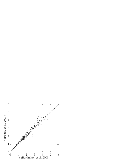
Figure 1: Cepheid distances found from the calibrations of Berdnikov et al. (2000) and Fouqu et al. (2007).

2 THE METHODS

2.1 Simultaneous Solution

This method for determining the kinematic parameters consists in minimizing a quadratic functional $F$:

$$\begin{array}[]{rll}\min~{}F&=&\sum_{j=1}^{N}w_{r}^{j}(V_{r}^{j}-\hat{V}_{r}^{j})^{2}\\ &+&\sum_{j=1}^{N}w_{l}^{j}(V_{l}^{j}-\hat{V}_{l}^{j})^{2}\end{array}$$ (4)

provided the fulfilment of the following constraints derived from Bottlinger’s formulas with an expansion of the angular velocity of Galactic rotation $\Omega$ into a series to terms of the second order of smallness with respect to $r/R_{0},$ and with allowance made for the influence of the spiral density wave:

$$\begin{array}[]{rll}V_{r}&=&-u_{\odot}\cos b\cos l\\ &-&v_{\odot}\cos b\sin l-w_{\odot}\sin b\\ &+&R_{0}(R-R_{0})\sin l\cos b\Omega^{\prime}_{0}\\ &+&0.5R_{0}(R-R_{0})^{2}\sin l\cos b\Omega^{\prime\prime}_{0}\\ &+&\tilde{v}_{\theta}\sin(l+\theta)\cos b,\\ &-&\tilde{v}_{R}\cos(l+\theta)\cos b,\end{array}$$ (5)

$$\begin{array}[]{rll}V_{l}&=&u_{\odot}\sin l-v_{\odot}\cos l\\ &+&(R-R_{0})(R_{0}\cos l-r\cos b)\Omega^{\prime}_{0}\\ &+&(R-R_{0})^{2}(R_{0}\cos l-r\cos b)\times\\ &\times&0.5\Omega^{\prime\prime}_{0}-r\Omega_{0}\cos b\\ &+&\tilde{v}_{\theta}\cos(l+\theta)+\tilde{v}_{R}\sin(l+\theta),\end{array}$$ (6)

where $N$ is the number of stars used; $j$ is the current star number; $V_{r}$ is the line-of-sight velocity, $V_{l}=4.74r\mu_{l}\cos b$ and $V_{b}=4.74r\mu_{b}$ are the proper motion velocity components in the $l$ and $b$ directions, respectively, with the coefficient 4.74 being the quotient of the number of kilometers in an astronomical unit and the number of seconds in a tropical year; $\hat{V}_{r}^{j},\hat{V}_{l}^{j}$ are the measured components of the velocity field (data); $w_{r}^{j}$ and $w_{l}^{j}$ are the weight factors; $r$ is the star’s heliocentric distance; the star’s proper motion components $\mu_{l}\cos b$ and $\mu_{l}\cos b$ and $\mu_{b}$ are in mas yr^-1 and the line-of-sight velocity $V_{r}$ is in km s^-1; $u_{\odot},v_{\odot},w_{\odot}$ are the stellar group velocity components relative to the Sun taken with the opposite sign (the velocity $u$ is directed toward the Galactic center, $v$ is in the direction of Galactic rotation, $w$ is directed to the north Galactic pole), we assume $w_{\odot}$ to be 7 km s^-1, because it is poorly determined without invoking the velocity components $V_{b}$; $R_{0}$ is the Galactocentric distance of the Sun; $R$ is the distance from the star to the Galactic rotation axis,

$$R^{2}=r^{2}\cos^{2}b-2R_{0}r\cos b\cos l+R^{2}_{0}.$$ (7)

$\Omega_{0}$ is the angular velocity of rotation at the distance $R_{0}$; the parameters $\Omega^{\prime}_{0}$ and $\Omega^{\prime\prime}_{0}$ are, respectively, the first and second derivatives of the angular velocity. To take into account the influence of the spiral density wave, we used the simplest kinematic model based on the linear density wave theory by Lin and Shu (1964), in which the potential perturbation is in the form of a travelling wave. Then

$$\begin{array}[]{rll}\tilde{v}_{R}&=&f_{R}\cos\chi,\\ \tilde{v}_{\theta}&=&f_{\theta}\sin\chi,\end{array}$$ (8)

where $f_{R}$ and $f_{\theta}$ are the amplitudes of the radial (directed toward the Galactic center in the arm) and azimuthal (directed along the Galactic rotation) velocity perturbations; the wave phase $\chi$ in general form is (Rohlfs 1977)

$$\chi=m[\Omega_{p}-\Omega(R)]t+\Phi(R),$$ (9)

where for a logarithmic spiral $\Phi(R)=\cot(i)\ln(R/R_{0})$, Eq. (9) for a fixed instant of time $t$ can be written as

$$\chi=m[\cot(i)\ln(R/R_{0})-\theta]+\chi_{\odot},$$ (10)

$f_{R}$ and $f_{\theta}$ enter into Eqs. (5) and (6) precisely for this approximation; $i$ is the spiral pitch angle ($i<0$ for winding spirals); $m$ is the number of arms, we take $m=2$ in this paper; $\theta$ is the star’s position angle (measured in the direction of Galactic rotation); $\chi_{\odot}$ is the Sun’s phase angle, measured here from the center of the Carina-Sagittarius spiral arm (R . 7 kpc), as was done by Rohlfs (1977). The parameter $\lambda$ is the distance (along the Galactocentric radial direction) between adjacent segments of the spiral arms in the solar neighborhood (the wavelength of the spiral density wave).it is calculated from the relation

$$\tan i={{\lambda m}\over{2\pi R_{0}}}.$$ (11)

The weight factors in functional (4) are assigned according to the following expressions (for simplification, we omit the index j):

$$\begin{array}[]{rll}w_{r}&=&S_{0}/\sqrt{S_{0}^{2}+\sigma^{2}_{V_{r}}},\\ w_{l}&=&\beta^{2}S_{0}/\sqrt{S_{0}^{2}+\sigma^{2}_{V_{l}}},\end{array}$$ (12)

where $S_{0}$ denotes the dispersion averaged over all observations, which has the meaning of a “cosmic” dispersion taken to be 12 km s^-1; $\beta=\sigma_{V_{r}}/\sigma_{V_{l}}=1$ is the scale factor that we determined using data on open star clusters (Bobylev et al. 2007). The errors of the velocities $V_{l}$ are calculated from the formula

$$\sigma_{V_{l}}=4.74r\sqrt{\mu^{2}_{l}\Biggl{(}{\sigma_{r}\over r}\Biggr{)}^{2}+\sigma^{2}_{\mu_{l}}}.$$ (13)

The optimization problem (4).(12) is solved for nine unknown parameters $u_{\odot},$ $v_{\odot},$ $\Omega_{0}$, $\Omega^{\prime}_{0},$ $\Omega^{\prime\prime}_{0},$ $f_{R},$ $f_{\theta},$ $i$ and $\chi_{\odot}$ by the coordinate-wise descent method.

We estimated the errors of the sought-for parameters through Monte Carlo simulations. The errors were estimated by performing 1000 cycles of computations. For this number of cycles, the mean values of the solutions essentially coincide with the solutions obtained from the input data without any addition of measurement errors. Measurements errors were added to such input data as the line-of-sight velocities, proper motions, and distances.

Here, we take a fixed value of R0 based on the review by Foster and Cooper (2010), where the weighted mean was $R_{0}=8.0\pm 0.4$ kpc.

Once the parameters of the rotation curve $\Omega(R),$ the perturbation amplitudes $f_{R}$ and $f_{\theta}$, and the pitch angle $i$ have been found from the solution of the system of equations (5), (6), we are able to determine $\Omega_{p}$. For this purpose, we use the approach applied by Mishurov et al. (1979). It is based on the assumption about an ellipsoidal distribution of residual stellar velocities. According to Lin et al. (1969),

$$f_{R}={kA\over\kappa}{\nu\over 1-\nu^{2}}F^{(1)}_{\nu}(x),$$ (14)

$$f_{\theta}=-{kA\over 2\Omega}{1\over 1-\nu^{2}}F^{(2)}_{\nu}(x),$$ (15)

where $A$ is the amplitude of the spiral density wave potential, $\kappa^{2}=4\Omega^{2}\left(1+{\displaystyle R\over\displaystyle 2\Omega}{\displaystyle d\Omega\over\displaystyle dR}\right)$ is the epicyclic frequency, $\nu=m(\Omega_{p}-\Omega)/\kappa$ is the frequency with which a test particle encounters the passing spiral perturbation, $k=m\cdot\cot(i)/R_{0}$ is the radial wave number, $F^{(1)}_{\nu}(x)$ and $F^{(2)}_{\nu}(x)$ are the reduction factors, which are functions of the coordinate $x=k^{2}\sigma^{2}_{R}/\kappa^{2},$, where $\sigma_{R}$ is the semimajor axis of the velocity ellipsoid. An expanded form of Eqs. (14) and (15) can be found in Mishurov et al. (1979).

Once Eqs. (14), (15) have been solved, we are able to estimate the ratio of the radial component of the gravitational force produced by the spiral arms to the total gravitational force of the Galaxy, $f_{r0},$, based on the well-known relation (Fernandez et al. 2008; Bobylev et al. 2011)

$$A=\frac{(R_{0}\Omega_{0})^{2}f_{r0}\tan i}{m}.$$ (16)

Our proposed approach to estimating the spiral pattern speed consists in finding the shifts in phase $\chi_{\odot}$ from several samples of stars with an age difference $\Delta t$ and to determine $\Omega_{p}$ from relation (9) for the known $\Omega(R_{0})$

$$\Delta\Omega=\Omega_{p}-\Omega(R_{0})={\Delta\chi_{\odot}\cdot 1000\over m\Delta t},$$ (17)

where the phase difference $\Delta\chi_{\odot}$ is in radians, and the age difference $\Delta t$ is in Myr. Note that the change in the Sun’s phase does not depend on the Galactic orbit of the Sun; we just find all of the parameters being determined for $R=R_{0}$ and, therefore, it would be more appropriate to call $\chi_{\odot}$ the phase of the solar circle.

2.2 Separate Approach

In the separate approach, a periodogram analysis based on the Fourier transform to determine the periodicities in the velocity components $V_{R}$ and $\Delta V_{rot}$ is used (Bobylev et al. 2008; Bobylev and Bajkova 2010). In this paper, we apply the method of Fourier analysis that takes into account the logarithmic pattern of the spiral density wave and the distribution of position angles $\theta$ (Bajkova and Bobylev 2012). .

Initially, we define the heliocentric components of the Cepheid space velocities $U$ and $V$ via the observed velocities $V_{r},V_{l},$ and $V_{b}$ based on the well-known relations

$$\begin{array}[]{rll}U&=&V_{r}\cos l\cos b-V_{l}\sin l-V_{b}\cos l\sin b,\\ V&=&V_{r}\sin l\cos b+V_{l}\cos l-V_{b}\sin l\sin b,\end{array}$$ (18)

Subsequently, we find two velocity components: the radial velocity $V_{R}$ directed from the Galactic center to the object and the tangential velocity $V_{\theta}$ in the direction of Galactic rotation:

$$\begin{array}[]{rll}V_{\theta}&=&U\sin\theta+(V_{0}+V)\cos\theta,\\ V_{R}&=&-U\cos\theta+(V_{0}+V)\sin\theta,\end{array}$$ (19)

where $V_{0}=|R_{0}\Omega_{0}|$ and the position angle $\theta$ is calculated as $\tan\theta=y/(R_{0}-x)$, where $x$ and $y$ are the heliocentric rectangular coordinates of the stars. Finally, based on the velocities $V_{\theta}$, we form the residual tangential velocities of the Cepheids $\Delta V_{rot}$ from which the rotation curve found above was subtracted.

In contrast to the previous method, here we do not assume that the wavelength $\lambda$ is the same for the velocity perturbations in the radial and tangential directions and that their phases $\chi_{\odot}$ differ exactly by $\pi/2$.

Below, we describe the method of spectral analysis of the radial velocity perturbations for objects both in the linear approximation of the dependence of the argument in (10) on Galactocentric distance and in its exact expression, i.e., by taking into account the logarithmic dependence on Galactocentric distance and position angle $\theta$.

Let there be a series of measured velocities $V_{R_{n}}$ (these can be both radial, $V_{R},$, and tangential, $\Delta V_{rot}$, velocities), $n=1,\dots,N$, where $N$ is the number of objects. The goal of the spectral analysis is to separate the periodicity from the data series in accordance with model (8)-(11), which describes a spiral density wave with parameters $f_{R},\lambda(i)$, and $\chi_{\odot}$.

Given relation (11) between the spiral pitch angle $i$ and wavelength $\lambda$ for $|R-R_{\circ}|\ll R_{\circ}$ and small $\theta$, the linear approximation for the logarithm of the argument in (10) can be represented as

$$\frac{2\pi R_{\circ}}{\lambda}\ln(R/R_{\circ})\approx\frac{2\pi(R-R_{\circ})}{\lambda}.$$

In this case, for our harmonic analysis of the velocities, we can apply the standard Fourier transform

$$\bar{V}_{\lambda_{k}}=\frac{1}{N}\sum_{n=1}^{N}V_{R_{n}}\exp\Bigl{(}-j\frac{2\pi}{\lambda_{k}}(R_{n}-R_{\circ})\Bigr{)},$$ (20)

where $\bar{V}_{\lambda_{k}}$ is the $k$th harmonic of the Fourier transform, $V_{R_{n}}$ are the velocity measurements for objects with Galactocentric distances $R_{n},n=1,2,...,N$, and $\lambda_{k}$ is the wavelength of the $k$th harmonic, which is equal to $D/k$, where $D$ is the period of the series being analyzed.

Since we are interested only in the perturbation power spectrum (periodogram) $|\bar{V}_{\lambda_{k}}|^{2}$ —, Eq. (20) can be simplified as follows:

$$\bar{V}_{\lambda_{k}}=\frac{1}{N}\sum_{n=1}^{N}V_{R_{n}}\exp\Bigl{(}-j\frac{2\pi}{\lambda_{k}}R_{n}\Bigr{)}.$$

Note that the derived linear approximation is acceptable only for analyzing the perturbations in a small solar neighborhood, while an exact realization of relation (10) is required for a wide scatter of distances and position angles for the objects.

Let us analyze the perturbations as a periodic function of the logarithm of the Galactocentric distances, for the time being, without allowance for the position angles of the objects:

$$\bar{V}_{\lambda_{k}}=\frac{1}{N}\sum_{n=1}^{N}V_{R_{n}}\exp\Bigl{(}-j\frac{2\pi R_{\circ}}{\lambda_{k}}\ln(R_{n}/R_{\circ})\Bigr{)}.$$ (21)

Obviously, if we make the change of variables

$$R^{{}^{\prime}}_{n}=\ln(R_{n}/R_{\circ})R_{\circ},$$ (22)

is reduced to the standard Fourier transform

$$\bar{V}_{\lambda_{k}}=\frac{1}{N}\sum_{n=1}^{N}V_{R^{{}^{\prime}}_{n}}\exp\Bigl{(}-j\frac{2\pi R^{{}^{\prime}}_{n}}{\lambda_{k}}\Bigr{)}.$$ (23)

To take the position angles of the objects into account, we will represent Eq. (10) for the phase as

$$\chi=\chi_{1}-m\theta,$$ (24)

where (given (11))

$$\chi_{1}=\frac{2\pi R_{\circ}}{\lambda}\ln(R/R_{\circ})+\chi_{\odot}.$$ (25)

Substituting (24) into Eq. (10) for the perturbations at the $n$th point and making standard trigonometric transformations, we will obtain:

$$\begin{array}[]{rll}&V_{R_{n}}=f_{R}\cos(\chi_{1_{n}}-m\theta_{n})\\ &=f_{R}\cos\chi_{1_{n}}\cos m\theta_{n}+f_{R}\sin\chi_{1_{n}}\sin m\theta_{n}\\ &=f_{R}\cos\chi_{1_{n}}(\cos m\theta_{n}+\tan\chi_{1_{n}}\sin m\theta_{n}).\end{array}$$ (26)

Let us designate

$$V_{R^{{}^{\prime}}}=f_{R}\cos\chi_{1},$$ (27)

It then follows from (26) that

$$V_{R_{n}}=V_{R^{{}^{\prime}}_{n}}(\cos m\theta_{n}+\tan\chi_{1_{n}}\sin m\theta_{n}).$$ (28)

Using Eq. (28), let us form a new data series

$$V_{R^{{}^{\prime}}_{n}}=V_{R_{n}}/(\cos m\theta_{n}+\tan\chi_{1_{n}}\sin m\theta_{n}),$$ (29)

to which a Fourier analysis can be applied in accordance with (23). A similar relation can also be derived for the tangential velocities $\Delta V_{rot}$.

Thus, taking into account both the logarithmic pattern of the spiral density wave and the position angles of the objects, we obtain the following expression for our spectral analysis of the perturbations:

$$\bar{V}_{\lambda_{k}}=\frac{1}{N}\sum_{n=1}^{N}V^{{}^{\prime}}_{R^{{}^{\prime}}_{n}}\exp\Bigl{(}-j\frac{2\pi R^{{}^{\prime}}_{n}}{\lambda_{k}}\Bigr{)}.$$ (30)

The numerical algorithm for realizing (30) consists of the following steps:

1. The initial series of velocities $V_{R_{n}}$ is transformed into the series $V_{R_{n}^{{}^{\prime}}}$ in accordance with (22).

2. The power spectrum of the derived sequence $V_{R_{n}^{{}^{\prime}}}$ is calculated based on the Fourier transform (23) to obtain an estimate of $\lambda_{max}$ that corresponds to the peak of the derived power spectrum.

3. A comb of several $\lambda_{i}(i=1,\dots,K)$ with a central $\lambda_{max}$ is then specified.

The following iterations are made for each $\lambda_{i}$ from the specified comb:

Step 1. The value of $\lambda_{i}$ and the initial approximation $\chi_{\odot}$ (for example, equal to zero) are substituted into Eq. (25) to calculate $\chi_{1}$ for each data reading ($n=1,\dots,N$).

Step 2. Using Eq. (29), the series of velocities $V_{R_{n}^{{}^{\prime}}}$ is transformed into the series $V^{{}^{\prime}}_{R^{{}^{\prime}}_{n}}$. This transformation needs to be regularized to avoid the division by numbers close to zero.This is done by assigning a threshold number, say, $\varepsilon$, and permission for the division is given only when the denominator in Eq. (29) exceeds this number. The best $\varepsilon$ at which the significance of the extracted peak in the spectrum reaches its maximum as a result of the iterations at the minimum residual between the solution and the data can be found by an exhaustive search for $\varepsilon$ from some interval. The typical values of $\varepsilon$ found on model problems lie within the range [0.01, 0.3].

Step 3. The power spectrum of the derived sequence $V^{{}^{\prime}}_{R^{{}^{\prime}}_{n}}$ is calculated based on the Fourier transform (30) to obtain a new estimate of $\chi_{\odot}$ corresponding to a fixed $\lambda_{i}$ of the derived power spectrum.

Step 4. The return to the first step is made until the process will converge or diverge.

Step 5. If the process converged, then we fix the specified $\lambda_{i}$ and the derived $\chi_{\odot}$; if it diverged, then we take the next value $\lambda_{i+1}$ from the specified comb and make iterations 1–4 until the value of $\lambda$ at which the process converges will be found.

4. The power spectrum is calculated for the values of $\lambda$ and $\chi_{\odot}$ found based on Eq. (30) with the goal of a further analysis.

A more detailed description of the algorithm, the results of its testing on model data, and the questions of estimating the significance of the extraction of peaks in the periodogram and estimating the errors in the spiral density wave parameters are given in Bajkova and Bobylev (2012).

Table 2: Kinematic parameters found from Cepheids

Parameters	$P\geq 9^{d}$	$5^{d}\leq P<9^{d}$	$P<5^{d}$	All
$u_{\odot},$ km s-1	$6.9\pm 1.2$	$7.5\pm 0.9$	$8.6\pm 1.3$	$7.6\pm 0.5$
$v_{\odot},$ km s-1	$11.6\pm 0.8$	$10.9\pm 0.6$	$15.6\pm 1.3$	$11.7\pm 0.3$
$\Omega_{0},$ km s-1 kpc-1	$26.1\pm 0.9$	$30.4\pm 1.0$	$24.1\pm 1.2$	$27.5\pm 0.5$
$\Omega^{{}^{\prime}}_{0},$ km s-1 kpc-2	$-3.95\pm 0.13$	$-4.34\pm 0.13$	$-4.72\pm 0.25$	$-4.12\pm 0.10$
$\Omega^{{}^{\prime\prime}}_{0},$ km s-1 kpc-3	$0.79\pm 0.10$	$0.69\pm 0.14$	$2.44\pm 0.28$	$0.85\pm 0.07$
$f_{R},$ km s-1	$-9.8\pm 1.3$	$-8.5\pm 1.1$	$-12.6\pm 1.7$	$-6.8\pm 0.7$
$f_{\theta},$ km s-1	$1.3\pm 1.9$	$2.7\pm 1.1$	$8.2\pm 1.4$	$3.3\pm 0.5$
$i,$ deg	$-5.2\pm 0.3$	$-4.0\pm 0.1$	$-6.6\pm 0.5$	$-4.6\pm 0.1$
$\chi_{\odot},$ deg	$-148\pm 14$	$-193\pm 9$	$-234\pm 10$	$-193\pm 5$
$\sigma_{0},$ km s-1	12.2	12.5	12.5	13.4
$\lambda,$ kpc	$2.3\pm 0.5$	$1.8\pm 0.1$	$2.9\pm 0.4$	$2.0\pm 0.1$
$N_{\star}$	61	72	52	185
$\overline{t}_{1}$, Myr	33.9	59.2	84.9
$\overline{t}_{2}$, Myr	55.4	95.2	135.0
$\sigma_{R},$ km s-1				14
$\Omega_{p}$, km s-1 kpc-1				23.5
$f_{r0}$				$0.04\pm 0.01$

Note: $N_{\star}$ is the number of Cepheids in the sample, $\sigma_{0}$ is the error per unit weight obtained when solving the system of equations (5),(6), $\sigma_{R}$ is the semimajor axis of the velocity ellipsoid, $\Omega_{p}$ was estimated by the method of Mishurov et al. (1979).

3 RESULTS AND DISCUSSION

3.1 Results of the Simultaneous Solution

The results of the solutions of the system of equations (5) and (6) obtained from four samples of Cepheids are presented in Table 2: for Cepheids with periods longer than 9 days, i.e., the youngest ones in our sample, in the first column; for Cepheids with periods from 5 to 9 days, i.e., middle-aged ones, in the second column; for Cepheids with periods shorter than 5 days, i.e., the oldest ones, in the third column; the solution obtained from all Cepheids is given in the fourth column.

The parameters of the Galactic rotation curve $\Omega_{0},$ $\Omega^{{}^{\prime}}_{0}$, and $\Omega^{{}^{\prime\prime}}_{0},$ calculated from the sample of middle-aged Cepheids are in good agreement with the results of analyzing blue supergiants (Zabolotskikh et al. 2002), OB associations (Mel’nik and Dambis 2009), and Galactic masers (Bobylev and Bajkova 2010; Stepanishchev and Bobylev 2011). In these papers, the angular velocity of Galactic rotation $\Omega_{0}$ is $\approx$30 km s^-1 kpc^-1. For unknown reasons, the youngest Cepheids revolve around the Galactic center with a lower velocity. Note that $\Omega_{0}$ and $\Omega^{{}^{\prime}}_{0},$ that we found based on the entire sample of Cepheids (the last column in Table 2) are in good agreement with the results of the analysis of only the proper motions of Cepheids from the Hipparcos catalog performed by Feast and Whitelock (1997), where $\Omega_{0}=27.2\pm 0.9$km s^-1 kpc^-1 was found.

It can be seen from Table 2 that the amplitudes of the velocity perturbations in the radial direction, $f_{R},$, differ significantly from zero in all cases, while in the tangential direction, $f_{\theta},$, they are significant for the sample of old Cepheids (and for the entire sample). The relationship between the amplitudes found is in agreement with the results of the analysis of blue supergiants performed by Zabolotskikh et al. (2002), $f_{R}=-6.6\pm 2.5$ km s^-1 and $f_{\theta}=0.4\pm 2.3$ km s^-1 for $m=2$, and a sample of young Cepheids with similar values of these parameters. Previously (Bobylev and Bajkova 2011), we found $f_{R}=-12.5\pm 1.1$ km s^-1, $f_{\theta}=2.0\pm 1.6$ km s^-1, and $i=-5.3\pm 0.3^{\circ}$ for $m=2$ with $\chi_{\odot}=-91\pm 4^{\circ}$ from data on OB3 stars with an independent distance scale determined from interstellar Ca II absorption lines.

In principle, the Sun’s phases found (Table 2) are consistent with the results of analyzing various samples of Cepheids, for example (with the phase measured from the Carina-Sagittarius arm): $\chi_{\odot}=-165\pm 1^{\circ}$ (Byl and Ovenden 1978), $\chi_{\odot}=-150^{\circ}$ from red supergiants and Cepheids (Mishurov et al. 1979), $\chi_{\odot}=-290\pm 16^{\circ}$ (Mishurov et al. 1997), and $\chi_{\odot}=-320\pm 9^{\circ}$ (Mishurov and Zenina 1999) from relatively old Cepheids with periods $P<9^{d}$.

In Figs. 2 and 3, the radial, $V_{R}$, and tangential, $V_{rot}=V_{\theta}$, velocities (calculated from Eqs. (19)) are plotted against the Galactocentric distance R for two samples of Cepheids.young and middle-aged ones. In each case, the rotation curve was constructed in accordance with the results of Table 2. A wave structure in the radial velocities $V_{R}$ is clearly seen in Figs.2 and 3.

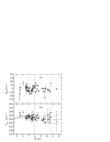
Figure 2: Radial velocities for the sample of young Cepheids (a) and their tangential velocities (b) versus Galactocentric distance R; the vertical dotted lines mark the Sun’s position, the solid curve in panel (b) indicates the rotation curve, the lines with long dashes mark the $1\sigma$ confidence intervals.

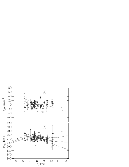
Figure 3: Radial velocities for the sample of middle-aged Cepheids (a) and their tangential velocities (b) versus Galactocentric distance R. The designations are the same as those in Fig. 2.

As can be seen from Table 2, the phase $\chi_{\odot}$ changes noticeably with the mean age of the sample. We also see that the mean Cepheid ages calculated using calibrations (2) and (3) differ by a factor of 1.5. Applying Eq. (17) gives $|\Delta\Omega|_{(1-2)}=9.9$ km s^-1 kpc^-1 (columns 1, 2, 3 in Table 2), $|\Delta\Omega|_{(2-3)}=9.4$ km s^-1 kpc^-1 and $|\Delta\Omega|_{(1-3)}=9.0$ km s^-1 kpc^-1 for the calibration of Efremov (2003) (Eq. (3)). In this case, the mean value of the difference $|\Delta\Omega|=9.4$ km s^-1 kpc^-1, then $\Omega_{p}=18.1$ km s^-1 kpc^-1 (for $\Omega_{0}=27.5\pm 0.5$ km s^-1 kpc^-1 found from the entire sample of Cepheids), which is in satisfactory agreement with the result obtained from Eqs. (14) and (15) by the method of Mishurov et al. (1979), $\Omega_{p}=23.5$ km s^-1 kpc^-1.

The analogous values found from the age calibration of Bono et al. (2005) (Eq. (2)) are considerably larger: $|\Delta\Omega|_{(1-2)}=15.4$ km s^-1 kpc^-1, $|\Delta\Omega|_{(2-3)}=14.7$ km s^-1 kpc^-1 and $|\Delta\Omega|_{(1-3)}=14.0$ km s^-1 kpc^-1. In this case, the mean value of the difference $|\Delta\Omega|=14.7$ km s^-1 kpc^-1, then $\Omega_{p}=12.8$ km s^-1 kpc^-1, which is in much poorer agreement with other known data.

Comparison of the results obtained allows us to opt for the age calibration of Efremov (2003).

The estimate of $f_{r0}=0.04\pm 0.01$ that we obtained from Eq. (16) is much smaller than $f_{r0}=0.15,$ found from a sample of 192 long-period Cepheids by Mishurov et al. (1979). At the same time, our estimate is in good agreement with $f_{r0}=0.05,$ suggested by Yuan (1969).

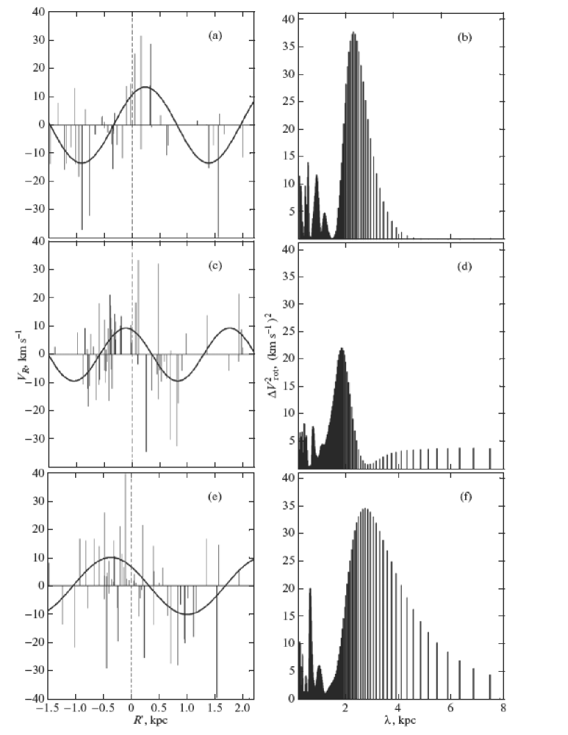
Figure 4: Radial velocities for the sample of young Cepheids (a) and their power spectrum (b), middle-aged Cepheids (c) and their power spectrum (d), and old Cepheids (e) and their power spectrum (f); the vertical dotted lines mark the Sun’s position.

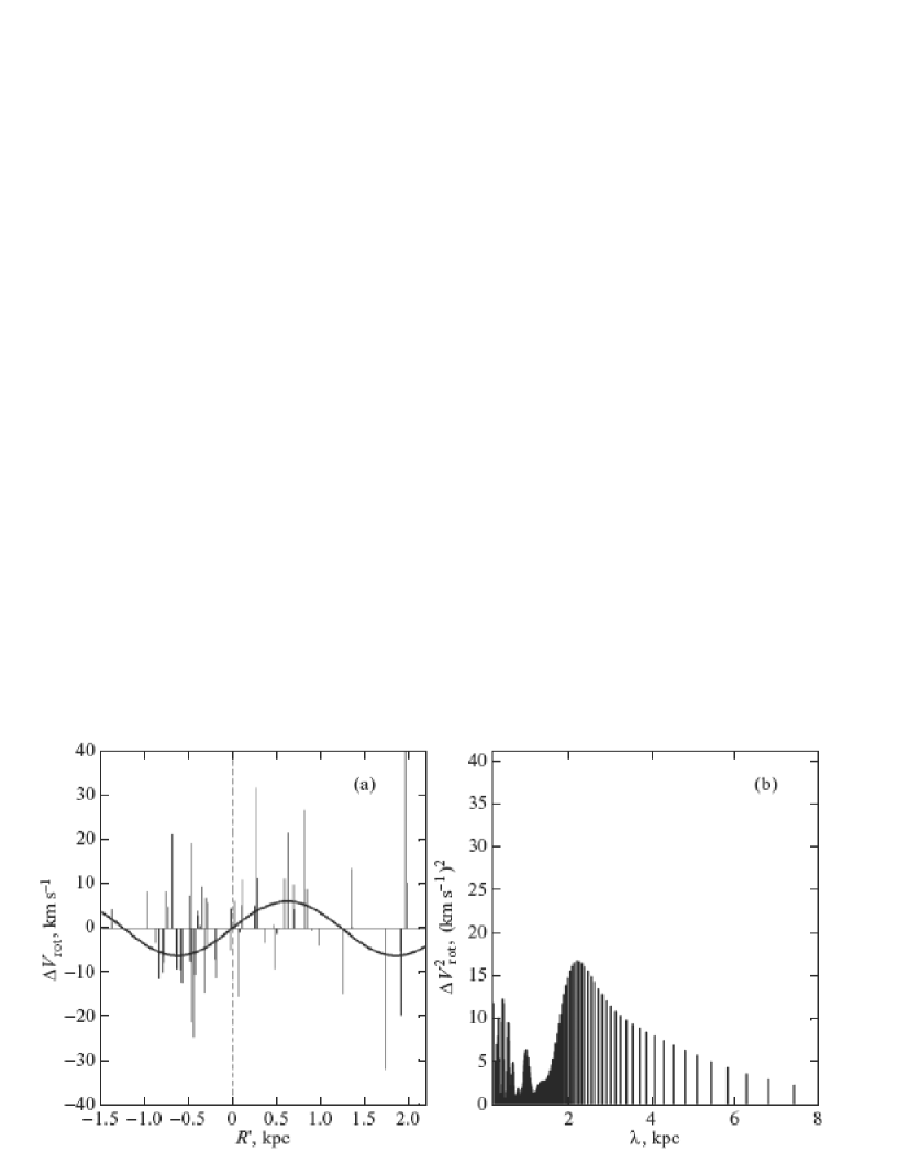
Figure 5: Residual tangential velocities for the sample of middle-aged Cepheids (a) and their power spectrum (b); the corresponding radial velocities are shown in panels (c and d) of Fig. 4.

3.2 Results of the Separate Approach

Figure 4 presents the Galactocentric radial velocities $V_{R}$ of the Cepheids and the corresponding power spectra. The distance $R^{{}^{\prime}}$ indicated in the plots was calculated from the relation $R^{{}^{\prime}}=\ln(R/R_{\circ})R_{\circ},$ which takes into account the logarithmic pattern of the spiral density wave (22). In contrast to Figs. 2 and. 3, the data here are presented in the form of “pulses” without indicating their random errors.

As in the previous case (Table 2), this approach failed to reveal a significant wave in the tangential velocities for the sample of the youngest Cepheids. The proposition of the density wave theory that the perturbations in the radial direction propagate faster than those in the tangential one can serve as an explanation of this fact. Therefore, the youngest stars have not yet had time to respond to the perturbations in the tangential direction, while the situation for the older stars gradually levels off.

Figure 5 shows the residual tangential velocities $\Delta V_{rot}$ for the sample of middle-aged Cepheids and their power spectrum.

We clearly see from Figs. 4 and 5 and the data of Table 2 that the wavelength $\lambda$ changes, depending on the sample and the velocity character. For example, the difference in $\lambda$ calculated from the radial and tangential velocities of middle-aged Cepheids is about 0.4 kpc. Comparison of the data in Fig. 5 with panels (c) and (d) in Fig. 4 leads us to conclude that there is a phase shift close to $\pi/2$ (the exact value is $110^{\circ}$), which is in agreement with the prediction of the linear density wave model. It can be seen from the sample of middle-ages Cepheids that the Sun is equidistant from the centers of the two nearest segments of the spiral arms.

For a more reliable determination of the mean $\Delta\Omega$, we invoked our previously obtained data on the kinematics of young OB3 stars (Bobylev and Bajkova 2011), where the Sun’s phase $\chi_{\odot}=-91\pm 4^{\circ}$ was obtained. For these stars, we took a mean age of 8 Myr. We calculated the mean $|\Delta\Omega|=9.8\pm 0.6$ km s^-1 kpc^-1 using six independent differences formed from four values of $\chi_{\odot}$: $-91^{\circ},$ $-148^{\circ},$ $-193^{\circ}$ and $-234^{\circ}.$ We used the mean Cepheid ages calculated from Efremov’s calibration. Here, the error $(\varepsilon_{\Delta\Omega})_{stat}=0.6$ km s^-1 kpc^-1 was calculated from the convergence of the results. We can also estimate the systematic error of the method, $(\varepsilon_{\Delta\Omega})_{syst},$ from the relation

$$(\varepsilon^{2}_{\Delta\Omega})_{syst}=1000^{2}\left(\left({\varepsilon_{\chi}\over m\Delta t}\right)^{2}+\left(-{\Delta\chi\cdot\varepsilon_{t}\over m(\Delta t)^{2}}\right)^{2}\right),$$ (31)

for the adopted typical values: $\varepsilon_{\chi}=10^{\circ}\cdot(\pi/180^{\circ}),$ $\Delta_{\chi}=50^{\circ}\cdot(\pi/180^{\circ}),$ $\Delta t=50$ Myr and $\varepsilon_{t}=10$ Myr, then $(\varepsilon_{\Delta\Omega})_{syst}=2.8$ km s^-1 kpc^-1. As a result, we have $|\Delta\Omega|=9.8\pm 0.6_{stat}\pm 2.8_{syst}$ km s^-1 kpc^-1.

Note that we found $\chi_{\odot}=-130\pm 10^{\circ}$ from a sample of masers in regions of active star formation (Bobylev and Bajkova 2010). Thus, they are intermediate between the OB3 stars and young Cepheids. Although there are no estimates of their individual ages, there are very massive O stars as well as high- and low-mass proto stars among them. The paradoxical value of $\chi_{\odot}=-130^{\circ}$ (the expected $\chi_{\odot}\approx-90^{\circ}$) can be explained by the fact that the kinematics of these recently formed stars probably reflects considerably earlier stages in the Galactic motion of the regions of active star formation.

The Galactic spiral pattern speed calculated by our proposed method from the entire sample of Cepheids ($\Omega_{0}=27.5$ km s^-1 kpc^-1) is $\Omega_{p}=17.7$ km s^-1 kpc^-1. If, however, we take $\Omega_{0}=30$ km s^-1 kpc^-1 known from our analysis of masers and OB3 stars, then we obtain $\Omega_{p}=20.2$ km s^-1 kpc^-1. According to these data, the co-rotation circle in the Galaxy is located at a distance from $R=$10 to 12 kpc. These estimates are valid for a two-armed Galactic spiral pattern ($m=2$). In the opinion of several authors, the Galactic spiral pattern is a four-armed one ($m=4$). In this case (see Eq. (17)), the difference we found will be $|\Omega_{p}-\Omega_{0}|\approx 5$ km s^-1 kpc^-1. Then, the spiral pattern speed will be $\Omega_{p}=22.5$ km s^-1 kpc^-1 from the entire sample of Cepheids ($\Omega_{0}=27.5$ km s^-1 kpc^-1) and $\Omega_{p}=25$ km s^-1 kpc^-1 for $\Omega_{0}=30$ km s^-1 kpc^-1; accordingly, the co-rotation circle will be still closer to the Sun.

4 CONCLUSIONS

We analyzed the space velocities of Galactic Cepheids to study the peculiarities of the Galactic spiral density wave. For this purpose, we used 185 Cepheids with proper motions mainly from the Hipparcos catalog and line-of-sight velocities from various sources. We divided the entire sample into three parts, depending on the pulsation period, which reflects well the mean Cepheid age.

First, based on the entire sample of Cepheids and taking $R_{0}=8$ kpc, we found the components of the peculiar solar velocity $(u_{\odot},v_{\odot})=(7.6,11.7)\pm(0.5,0.3)$ km s^-1, the angular velocity of Galactic rotation $\Omega_{0}=27.5\pm 0.5$ km s^-1 kpc^-1 and its derivatives $\Omega^{{}^{\prime}}_{0}=-4.12\pm 0.10,$ km s^-1 kpc^-2 and $\Omega^{{}^{\prime\prime}}_{0}=0.85\pm 0.07,$ km s^-1 kpc^-3, the amplitudes of the spiral density wave $f_{R}=-6.8\pm 0.7$ km s^-1 and $f_{\theta}=3.3\pm 0.5$ km s^-1, the pitch angle of a two-armed spiral pattern $i=-4.6\pm 0.1^{\circ}$ (then $\lambda=2.0\pm 0.1$ kpc), and the phase of the Sun in the spiral density wave $\chi_{\odot}=-193\pm 5^{\circ}$.

The Cepheids with pulsation periods $P$ from 5 to 9 days (middle-aged) ($\Omega_{0}=30.4\pm 1.0$ km s^-1 kpc^-1 for them) show the fastest Galactic rotation. The amplitude of the radial velocity perturbations $f_{R}$ caused by the spiral density wave in each of the three samples is about 9 km s^-1; the amplitude of the tangential velocity perturbations $f_{\theta}$ increases from zero for the youngest Cepheids to $\approx$4 km s^-1 for older ones.

We found that the Sun’s phase $\chi_{\odot}$ changes noticeably with the mean age of the sample. For a more accurate estimation of the phase, we applied a Fourier analysis of the Cepheid radial velocities, while for middle-aged Cepheids we also managed to reliably determine the parameters of the tangential velocity perturbations by this method.

From our analysis of the phase shifts, we determined the mean value of the angular velocity difference $\Delta\Omega=\Omega_{p}-\Omega$, which depends significantly on the calibrations used to estimate the individual ages of Cepheids. For a more reliable determination of the mean $\Delta\Omega$, we invoked our previously obtained data on the kinematics of young OB3 stars. As a result, we calculated the mean $\Delta\Omega$ using six independent differences.

We showed that when the individual ages of Cepheids derived from the period-age calibration of Bono et al. (2005) is used, the differences $\Omega_{p}-\Omega_{0}$ exceed those derived from the calibration of Efremov (2003) by a factor of 1.5-2. Simultaneously, we obtained an estimate of $\Omega_{p}=23.5$ km s^-1 kpc^-1 from our analysis of the reduction factors by the method of Mishurov et al. (1979). As a result, this allowed us to opt for Efremov’s calibration , using which we found $|\Omega_{p}-\Omega_{0}|=9.8\pm 0.6_{stat}\pm 2.8_{syst}$ km s^-1 kpc^-1.

The Galactic spiral pattern speed that we calculated by our proposed method based on the entire sample of Cepheids ($\Omega_{0}=27.5$ km s^-1 kpc^-1) is $\Omega_{p}=17.7$ km s^-1 kpc^-1. If, however, we take $\Omega_{0}=30$ km s^-1 kpc^-1 known from our analysis of masers and OB3 stars, then we will obtain $\Omega_{p}=20.2$ km s^-1 kpc^-1. According to these data, the co-rotation circle in the Galaxy is located at a distance from R = 10 to 12 kpc.

Based on the entire sample of Cepheids, we estimated the ratio of the radial component of the gravitational force produced by the spiral arms to the total gravitational force of the Galaxy to be $f_{r0}=0.04\pm 0.01$.

5 ACKNOWLEDGMENTS

We are grateful to the referees for valuable remarks that contributed to a significant improvement of the paper. This work was supported in part by the “Nonstationary Phenomena in Objects of the Universe” Program of the Presidium of the Russian Academy of Sciences and grant no. NSh-1625.2012.2 from the President of the Russian Federation. In our work, we used the SIMBAD search database and the DDO Cepheid database.

6 REFERENCES

1. I. A. Acharova, Yu. N. Mishurov, and V. V. Kovtyukh, Mon. Not. R. Astron. Soc. 420, 1590 (2012).

2. A. T. Bajkova and V. V. Bobylev, Astron. Lett. 38, 549 (2012).

3. L. N. Berdnikov, A. K. Dambis, and O. V. Vozyakova, Astron. Astrophys. Suppl. Ser. 143, 211 (2000).

4. V. V. Bobylev, A. T. Bajkova, S. V. Lebedeva, Astron. Lett. 33, 720 (2007).

5. V. V. Bobylev, A. T. Bajkova, and A. S. Stepanishchev, Astron. Lett. 34, 515 (2008).

6. V.V.Bobylev, andA.T. Bajkova,Mon. Not.R. Astron. Soc. 408, 1788 (2010).

7. V. V. Bobylev and A. T. Bajkova, Astron. Lett. 37, 526 (2011).

8. V. V. Bobylev, A. T. Bajkova, A. Myllari, and M. Valtonen, Astron. Lett. 37, 550 (2011).

9. G. Bono, M. Marconi, S. Cassisi, et al., Astrophys. J. 621, 966 (2005).

10. J. Byl and M. W. Ovenden, Astrophys. J. 225, 496 (1978).

11. Yu. N. Efremov, Astron.Rep. 47, 1000 (2003).

12. M. Feast and P.Whitelock, Mon. Not. R. Astron. Soc. 291, 683 (1997).

13. D. Fernandez, F. Figueras, and J. Torra, Astron. Astrophys. 480, 735 (2008).

14. T. Foster and B. Cooper, ASP Conf. Ser. 438, 16 (2010).

15. P. Fouqu, P. Arriagada, J. Storm, et al., Astron. Astrophys. 476, 73 (2007).

16. O. Gerhard, Mem. Soc. Astron. Ital. Suppl. 18, 185 (2011).

17. G. A. Gontcharov, Astron. Lett. 32, 759 (2006).

18. E. Hog, C. Fabricius, V. V. Makarov, et al., Astron. Astrophys. 355, L27 (2000).

19. F. van Leeuwen, Astron. Astrophys. 474, 653 (2007).

20. C. C. Lin and F. H. Shu, Astrophys. J. 140, 646 (1964).

21. C. C. Lin, C. Yuan, and F. H. Shu, Astrophys. J. 155, 721 (1969).

22. A. M. Mel’nik, A. K. Dambis, and A. S. Rastorguev, Astron. Lett. 25, 518 (1999).

23. A. M. Mel’nik and A. K. Dambis, Mon. Not. R. Astron. Soc. 400, 518 (2009).

24. Yu. N. Mishurov, I. A. Zenina, A. K. Dambis, et al., Astron. Astrophys. 323, 775 (1997).

25. Yu. N. Mishurov, E. D. Pavlovskaya, and A. A. Suchkov, Sov. Astron. 23, 147 (1979).

26. Yu. N.Mishurov and I. A. Zenina, Astron. Astrophys. 341, 81 (1999).

27. M. E. Popova, Astron. Lett. 32, 244 (2006).

28. A.S.Rastorguev,E. V. Glushkova, A. K. Dambis, and M. V. Zabolotskikh, Astron. Lett. 25, 595 (1999).

29. K. Rohlfs, Lectures on Density Wave Theory (Springer, Berlin, 1977).

30. A. S. Stepanishchev and V. V. Bobylev, Astron. Lett. 37, 254 (2011).

31. C. Yuan, Astrophys. J. 158, 889 (1969).

32. M. V. Zabolotskikh, A. S. Rastorguev, and A. K. Dambis, Astron. Lett. 28, 454 (2002).

33. N. Zacharias, C. Finch, T. Girard, et al., CDS Strasbourg, I/315 (2009)

34. The Hipparcos and Tycho Catalogues, ESA SP-1200 (1997).