Mosaiced wide-field VLBI observations of the Lockman Hole/XMM

Active Galactic Nuclei (AGN) play a decisive role in galaxy evolution, particularly so when operating in a radiatively inefficient mode, where they launch powerful jets that reshape their surroundings. However, identifying them is difficult, since radio observations commonly have resolutions of between 1 arcsec and 10 arcsec, which is equally sensitive to radio emission from star-forming activity and from AGN. Very Long Baseline Interferometry (VLBI) observations allow one to filter out all but the most compact non-thermal emission from radio survey data. The observational and computational demands to do this in large surveys have been, until recently, too high to make such undertakings feasible. Only the recent advent of wide-field observing techniques have facilitated such observations, and we here present the results from a survey of 217 radio sources in the Lockman Hole/XMM field. We describe in detail some new aspects of the calibration, including primary beam correction, multi-source self-calibration, and mosaicing. As a result, we detected 65 out of the 217 radio sources and were able to construct, for the first time, the source counts of VLBI-detected AGN. The source counts indicate that at least 15 %–25 % of the sub-mJy radio sources are AGN-driven, consistent with recent findings using other AGN selection techniques. We have used optical, infrared and X-ray data to enhance our data set and to investigate the AGN hosts. We find that among the sources nearby enough to be resolved in the optical images, 88 % (23/26) could be classified as early-type or bulge-dominated galaxies. While 50 % of these sources are correctly represented by the SED of an early-type galaxy, for the rest the best fit was obtained with a heavily extinct starburst template. However, this is due to a degeneracy in the fit, as such extinction in the templates is mimicking early-type objects. Overall, the typical hosts of VLBI-detected sources are in good agreement with being early-type or bulge-dominated galaxies.

1 Introduction

It has recently become clear that the formation and evolution of galaxies is significantly influenced by the presence of active galactic nuclei (AGN). The large amounts of radiation produced by AGN can heat the interstellar gas in galaxies so that star formation is slowed down (e.g., Di Matteo et al. 2005), but the ejecta from AGN can also compress interstellar gas and trigger star formation (e.g., Gaibler et al. 2012). It is therefore important to determine if an AGN is present or not, but this is a difficult undertaking. Unambiguous identifications of AGN are difficult to make, since the AGN can be shielded from our view at most wavelengths, and so a non-detection does not imply that an AGN is not present.

An exception is the radio regime – even the most dust-rich galaxies are transparent at GHz frequencies, and so sensitive radio surveys of large portions of the sky have become an indispensable ingredient in the melting pot of contemporary extragalactic surveys. They provide information about thermal and non-thermal emission and on kpc-scale morphology, and so yield clues about the stellar and accretion activity in galaxies. The angular resolution of surveys carried out with compact interferometers, however, is insufficient to reliably infer the emission processes at work if the objects are unresolved (which most of them are with arcsec resolution), and so we are non the wiser.

Fortunately, observations using the Very Long Baseline Interferometry (VLBI) technique provide characteristics which help with the identification of radio-emitting AGN. The long baselines provide milli-arcsecond-scale resolution, which implies that the emission required to make a detection comes from very small volumes, which in turn implies that the brightness temperatures of these regions must be high (of order $10^{6}$ K). Such brightness temperatures generally can only be reached by AGN or extremely bright supernovae (Kewley et al. 2000), but if one observes objects at redshifts larger than $z=0.1$ one finds that the luminosity required for a detection exceeds that of stellar non-thermal sources, and one can be confident that an AGN has been detected. In nearby objects, non-thermal sources such as supernova remnants can be bright enough for VLBI studies.

But VLBI observations traditionally target single, carefully selected objects, because of the computational challenges inherent in imaging larger fields (Garrett et al. 2005; Lenc et al. 2008) and because objects which provide the high brightness temperatures required to make detections are sparsely distributed on the sky. Recent technical progress, however, have made it feasible to carry out the required calculations to image larger fields (Deller et al. 2007, 2011), and have facilitated bandwidth upgrades resulting in substantial sensitivity improvements. Therefore imaging wide fields with VLBI techniques has become feasible, and first exploratory projects have proven to be successful (Middelberg et al. 2011a; Morgan et al. 2011). VLBI observers finally have the chance to carry out surveys of large portions of the sky.

However, the aforementioned experiments did fall short of matching typical wide, deep radio surveys because they only used single pointings and required sources with substantial flux density in their fields to enable self-calibration of the data, required to reach the full sensitivity of the observations. We therefore embarked on a project to test the feasibility of surveying fields which are larger than a single pointing and which do not contain suitable in-beam calibrators. The Very Long Baseline Array (VLBA) was the instrument of choice, since it has equal antennas, simplifying the calibration, and the antennas are small (25 m) resulting in comparatively large primary fields of view.

This paper is structured as follows. Section 1.1 describes the selection of the target field; Sect. 2 describes the observations and Sect. 3 the calibration of the data, including several new aspects required in wide-field VLBI observations. Section 4 presents the imaging and image analysis and Sect. 5 contains an analysis of the results, detailing the fraction of detected sources, radio source counts, and properties of the host galaxies. Section 6 summarises these results, and Appendix A contains catalogues, contour plots and RGB images of the detected sources.

1.1 Field selection

Table 1: Candidate field parameters. Given are the number of sources found in arcsec resolution observations at 1.4 GHz, $N_{\rm src}$, the field declination, quality of the multi-wavelength coverage, the separation to the nearest listed calibrator and the availability of a potential in-beam calibrator.

Field name	$N_{\rm src}$	Declination	coverage	ext. cal.	in-beam cal.
Lockman Hole/XMM (Ibar et al. 2009)	1450	$+57^{\circ}$	good	1.27∘	possible
COSMOS (Schinnerer et al. 2007)	3643	$+2^{\circ}$	superb	3.01∘	no
ATLAS/CDFS (Norris et al. 2006)	726	$-28^{\circ}$	superb	1.87∘	yes
Subaru/XMM (Simpson et al. 2006)	512	$-5^{\circ}$	good	1.46∘	possible
Lockman Hole/North (Owen & Morrison 2008)	2056	$+59^{\circ}$	poor	2.23∘	no
ELAIS N2 (Ciliegi et al. 1999)	305	$+41^{\circ}$	medium	1.49∘	possible
ELAIS N1 (Ciliegi et al. 1999)	361	$+54^{\circ}$	medium	2.24∘	possible

Even though this project aimed at further developing VLBI survey techniques, care was taken to ensure an adequate interpretation of the results. Hence, to maximise the output of this project a field was selected based on (i) visibility, (ii) coverage at other wavelengths, and (iii) availability of calibrators, inside and outside the field (here a calibrator source is any source with an arcsec-scale flux density of tens of mJy, but no information was available if that source would be sufficiently compact for VLBI observations). The candidates along with a few of their characteristics are shown in Table 1, ranked in descending order of suitability. The COSMOS area is quite far away from a listed source suitable for external calibration and there is no sufficiently strong source in the field; ATLAS/CDFS is very far south; Subaru/XMM is far south and has relatively shallow arcsec-resolution coverage; Lockman Hole/North does not have good coverage at other wavelengths and was deliberately chosen to avoid strong sources (i.e., potential calibrators); and the ELAIS fields have too shallow arcsec-resolution coverage.

Therefore the Lockman Hole/XMM field was targeted, at declination $+57^{\circ}$. An overview of the radio observations is shown in Fig. 1. Complementary data include GMRT 610 MHz data, providing spectral indices (or limits) for all sources; deep Spitzer/SWIRE data (Lonsdale et al. 2003); deep XMM data (Brunner et al. 2008); and optical coverage with the Large Binocular Telescope and the Subaru telescope (Barris et al. 2004; Rovilos et al. 2009; Fotopoulou et al. 2012). Furthermore, very deep 3.6 $\mu$m and 4.5 $\mu$m data from the Spitzer/SERVS mission (Mauduit et al. 2012), and very deep 250 $\mu$m-500 $\mu$m data from the HERMES will be available soon. These data are crucial for selecting galaxies with matching properties and to disentangle the contributions of AGN to the bolometric luminosity.

Only sources with integrated flux densities of more than 100 $\mu$Jy were targeted in our observations, because it was expected that the noise in the combined VLBA images would reach around 20 $\mu$Jy beam^-1. Of the input sample, 496 sources met this criterion and were located within 20 arcmin of any of the pointing centres. However, after calibration only 217 were found to be in principle detectable, because their VLA flux densities exceeded 6 times the local noise level (see Sect. 5 for details). An overview of the 3 VLBA pointings, along with the location of target sources, is shown in Fig. 1, and a histogram of the source flux densities is shown in Fig. 2.

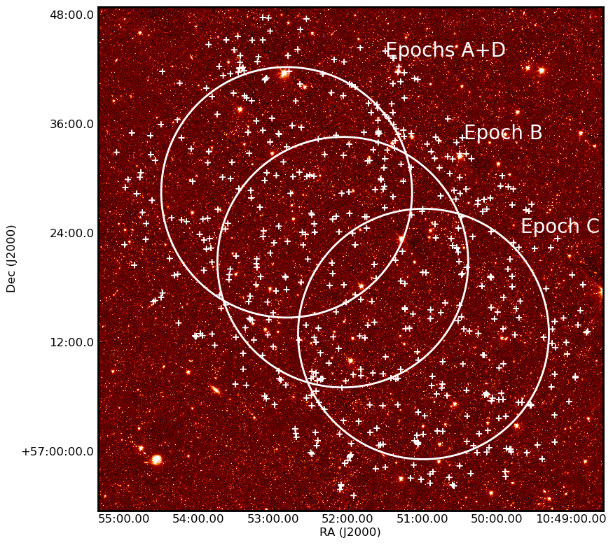
Figure 1: Overview of the Lockman Hole/XMM observations. Shown is the Spitzer 3.6 $\mu$m image as colour scale in the background. The three circles denote the FWHM of the VLBA antennas’ primary beams. The pointing coordinates have been taken from the VLA observations of this field reported in Ibar et al. (2009). Also indicated are which pointings have been observed in epochs A to D. Crosses indicate radio sources from Ibar et al. (2009) with a flux density of 100 $\mu$Jy or more, and located within 20 arcmin of a pointing centre.

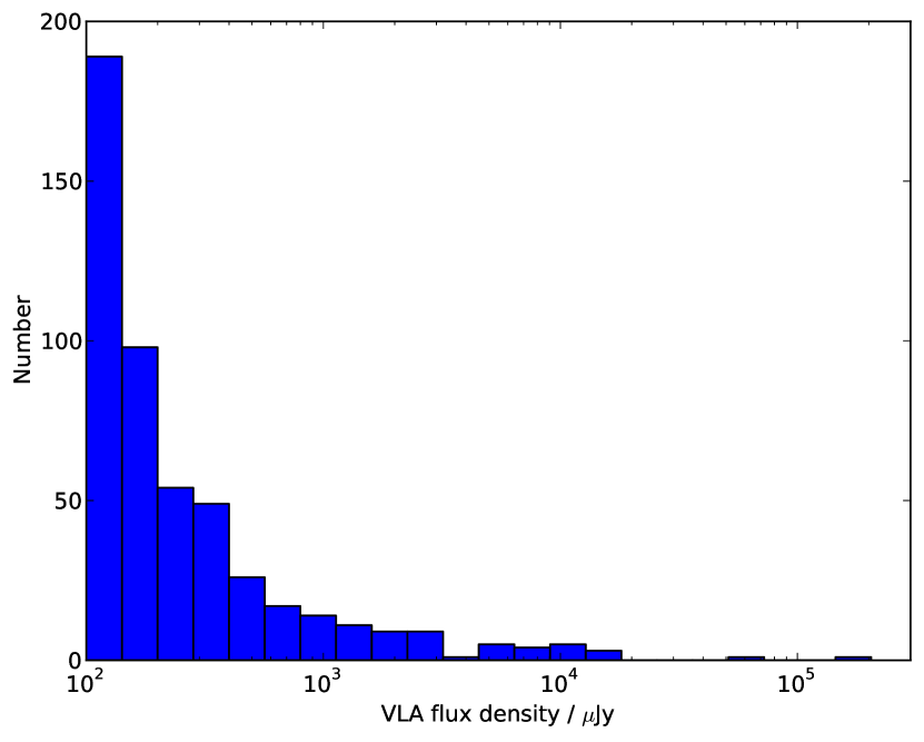
Figure 2: Distribution of VLA source flux densities in bins with edges at 100 $\mu$Jy$\times\sqrt{2}^{N}$, $N=0,1,2,...$

2 Observations

The observations for this project were carried out with the VLBA at 1.382 GHz on 3 June (epoch A), 4 July (epoch B), 16 July (epoch C) and 3 September (epoch D) of 2010. A recording bitrate of 512 Mbps was used, resulting in a bandwidth of 64 MHz in two parallel-hand polarisations, yielding a nominal sensitivity of around 24 $\mu$Jy beam^-1 towards the pointing centre. The fringe-finder 4C 39.25 was observed every 2.5 h for data consistency checks, and the fields were observed for 4.5 min, followed by a 1 min observation of the phase-referencing source NVSS J105837+562811. The elapsed time of the observations was 12 h per epoch, resulting in a total on-source time of around 326 baseline-hours per epoch. The VLBA observational status summary predicts a baseline sensitivity of 3.3 mJy in a 2 min observations with a recording rate of 256 Mbit, scaling to an image sensitivity of

$$\sigma=\frac{3.3\,{\rm mJy}}{\sqrt{\frac{512\,{\rm Mbps}}{256\,{\rm Mbps}}}\sqrt{\frac{60\,{\rm min}}{2\,{\rm min}}}\sqrt{326}}=23.6\,\mu{\rm Jy}$$ (1)

A pre-production version of VLBA-DiFX was used to correlate the data, using the new multi-field-centre mode. A memory leak in an associated program (difx2fits, which converts the data from the internal DiFX format to FITS-IDI) caused the loss of the first half of the data of the epoch A observations, which was overwritten with the second half. This was only discovered after the raw data had already been deleted, and a recorrelation was not possible. A reobservation of epoch A was requested and granted (epoch D), so that one of the three pointings in the Lockman Hole/XMM region now has deeper coverage than the other two. Correlation of the data resulted in approximately 320 data sets per epoch, each with a spectral resolution of 500 kHz and 4 s integrations. Since the field of view of each data set is centred on the known position of a VLA-detected source the field of view to be imaged is relatively small, and bandwidth and time smearing are not an issue (see Morgan et al. 2011 for a detailed description of these effects). The data volume was around 1 GB per source, per epoch.

3 Calibration

3.1 Standard steps

The calibration followed standard procedures used in phase-referenced VLBI observations, using the Astronomical Image Processing System, AIPS, with its Python interface, ParselTongue (Kettenis et al. 2006). Amplitude calibration was carried out using $T_{\rm sys}$ measurements and known gain curves. Fringe-fitting was carried out on the phase calibrator directly, to compensate for residual delays, without fringe-fitting the fringe finder (4C39.25) first, as would normally be done (a bug in the VLBA electronics causes unpredictable delay jumps in observations using a recording rate of 512 Mbps and 8 MHz IFs, and fringe finder observations are too infrequent to keep track of these jumps). However, the phase calibrator was bright enough to be detected separately in each IF channel during the 1 min scans, and so there was no need to use the fringe finders.

3.2 Multi-field self-calibration

After fringe fitting the delay and phase corrections were copied to the individual data files. In phase-referenced observations such as this the SNR typically is limited by ionospheric and atmospheric turbulence between calibrator scans, and therefore purely phase-referenced images have reduced coherence. When the target is sufficiently strong, self-calibration can be used to improve coherence, but here the targets were too faint. However, the combined flux density of the strongest few targets would be sufficient to carry out phase self-calibration. This has already been pointed out by Garrett et al. (2004), but had never been demonstrated in practice. We describe here a simple procedure which implements multi-field self-calibration.

• Phase-referenced images were made of all targets, and the images were searched for emission. Typically around 30 sources were found with a SNR of more than 7, with the brightest reaching an SNR of almost 100. The data are later combined using weights which are proportional to the square of the SNR, hence a source with SNR=10 contributes only 1/100 of the combined signal compared to a source with SNR=100. Therefore only the brightest 10 sources or so were used in the following steps.

• The individual data sets were divided by the CLEAN model obtained during imaging. This results in data sets each showing a 1 Jy point source in the field centre. It is worth noting that in this process the data weights are modified by the inverse square of the amplitude adjustment, and so this procedure conveniently takes care of proper weighting when the data are combined.

• The source coordinates in the data set headers were set to the same value. Subsequently, the data were concatenated into a single data set. For each baseline, time, and frequency the combined data now contains multiple measurements of a point source.

• Self-calibration was used with a 1 Jy point source model to improve the coherence of the combined data set. The phase corrections derived in this process were then copied to all original data sets, and improved images could be made.

The improvement attainable with this technique is illustrated in Fig. 3.

Figure 3: Contour plot of the radio source L0412 before (left) and after (right) multi-source self-calibration has been applied. Contours are drawn at 0.1 mJy$\times$(1, 2, 4, …). The signal-to-noise ratio was improved from 72 to 115. The peak flux density has increased significantly, the noise has dropped, and image artifacts are much reduced. These effects will be more pronounced when the initial calibration is not as good as in this case, for example, when a field at low elevation is observed.

3.3 Mosaicing

After multi-field self-calibration the calibration of each individual epoch was considered to be complete, and the data from the various epochs needed to be combined to reach maximum sensitivity. Two effects needed to be calibrated before combining the data: a potential systematic astrometric offset, and the primary beam attenuation.

Astrometric offsets between the epochs arise from a number of effects. First, unmodelled propagation delays (e.g., due to tropospheric water vapour, or the ionosphere) will vary between epochs and lead to a different residual phase error at the target field. Secondly, any component of these unmodelled propagation effects which is constant over long timescales will introduce further errors which differ between epochs, since the separation between phase calibrator and target field changes between epochs. And third, the in-beam calibrators will all have modelled positions and structure which differ from their true properties due to the limited S/N during the initial image reconstruction and differential phase calibration effects across the target field. The necessary usage of different sets of in-beam calibrators for multi-source selfcal in the different pointings will introduce different, small errors between the epochs.

To measure and calibrate a potential systematic offset a set of 18 sources was selected from epoch B which were also found in epochs A/D and C (but not all sources were present in all data epochs). These sources were imaged after multi-field self-calibration and the images were searched for the brightest pixels. The position differences relative to epoch B were calculated and the median used as the best approximation of a systematic offset between epochs A/C/D and B. The median offsets were found to be less than 1 mas in all cases, while the resolution of the images was around $10\,{\rm mas}\times 8\,{\rm mas}$. Correction of the offsets before the data were combined resulted in an increase of the peak flux densities of the calibrator sources of around 1 %, compared to a trial run in which the data were combined without offset correction. The mean offsets of epochs A/C/D relative to B before and after correction are listed in Tab. 2.

Table 2: Average position offsets relative to epoch B before and after position correction.

	before correction		after correction
	$\Delta$RA	$\Delta$Dec	$\Delta$RA	$\Delta$Dec
	mas	mas	mas	mas
B–A	$-0.17$	$1.40$	$0.19$	$-0.20$
B–C	$-0.46$	$-0.67$	$0.00$	$-0.08$
B–D	$-0.17$	$-1.00$	$0.00$	$0.00$

3.4 Primary beam corrections

The primary beam correction scheme used here has been described in detail in Middelberg et al. (2011a), who noted that the accuracy of the scheme was unknown, and they estimated its errors to be of the order of 10 %. We present here the results of an experiment to improve the quality of the corrections and to assess their accuracy.

On 21 September 2011, a pattern of pointing positions around 3C 84 was observed with the VLBA at 1.382 GHz to measure the primary beam response of the antennas. The frequency setup was identical to the VLBA observations of the CDFS by Middelberg et al. (2011a) and the Lockman Hole/XMM.

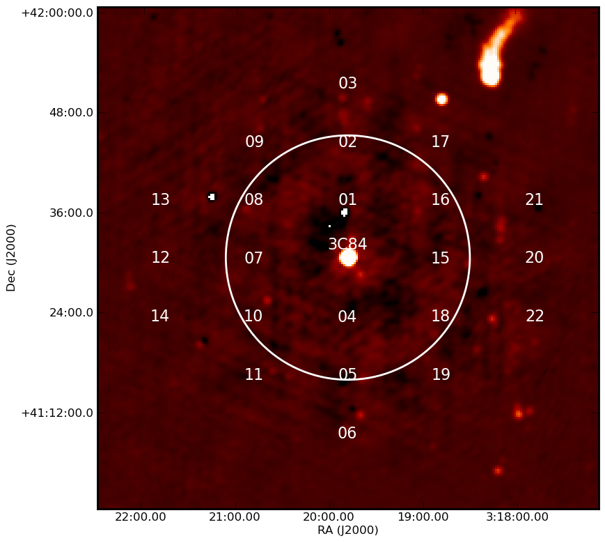
Figure 4: Locations of the antenna pointing positions used to test the primary beam attenuation of the VLBA antennas, shown on top of an NVSS postage stamp. 3C 84, in the image centre, has always been used as the field centre in the correlation, so that it was seen by the antennas through the various parts of the primary beam power pattern, the FWHM of which is indicated by the circle.

The pattern of pointings used for this experiment is shown in Fig. 4. The antennas were pointed towards each position for 1 min, except for the central pointing which was observed five times for 1.5 min for amplitude reference. Correlation has been performed using the true position of 3C 84 for all pointings, hence the amplitudes were only affected by primary beam effects. Initial amplitude calibration was carried out using $T_{\rm sys}$ measurements and known antenna gain curves. Fringe-fitting using the data from all pointings was used to correct phase and delay errors. The data from the central 1.5 min scan of 3C 84 was then imaged to obtain an approximate Stokes I model for further calibration. Amplitude self-calibration was subsequently carried out using this model to correct for residual amplitude variations and in particular to remove amplitude differences between RCP and LCP (assuming 3C 84 is circularly unpolarised, which, according to Homan & Wardle 2004, is the case at frequencies below 15 GHz). These corrections were then applied to the data from all pointing positions, so that amplitude variations should exclusively be caused by primary beam attenuation. Images were then made of all pointings and the flux densities of the brightest image pixels were extracted. Note that for an image of the pointing centred on the true position of 3C 84 only the centre scan was used to eliminate effects arising from a better $(u,v)$ coverage for this pointing.

The uncorrected peak flux densities are shown in Fig. 5 as a function of distance to the 3C 84 position. Two models have been used to reproduce these measurements, a Gaussian and an Airy disk. A Gaussian can be used effectively to model the inner portion of an antenna’s power pattern, since it is a good approximation and has a convenient and familiar parameter to represent its properties, which is the full width at half maximum (FWHM). However, it does a poor job near and beyond the first null of the antenna power pattern, and increasingly deviates from this simple model. A relatively obvious starting point for an improved model is the Airy disk, which essentially is a Bessel function. To first order an antenna can be treated as a uniformly illuminated disk, the Fraunhofer diffraction pattern of which is given by

$$I(\theta)=I_{0}\times\left(\frac{2J_{1}(\frac{\pi}{\lambda}D\sin\theta)}{\frac{\pi}{\lambda}D\sin\theta}\right)^{2}$$ (2)

where $J_{1}(x)$ is the Bessel function of order one, $\lambda$ is the observing wavelength, $D$ is the diameter of the aperture, and $\theta$ is the direction in which the intensity is to be calculated. Since only deviations from the on-axis sensitivity are to be calculated, $I_{0}$ can be set to one and ignored. Both the Gaussian and the Airy disk model have been fitted to the data; in the case of the Gaussian the FWHM has been allowed to vary and in the case of the Airy disk model the antenna diameter was allowed to vary (and the wavelength was kept constant). Since the antenna feed horns potentially only illuminate a part of the dish or, conversely, can illuminate a solid angle which extends beyond it, the effective dish diameter can differ slightly from the geometric aperture. It therefore is more appropriate to solve for the effective dish diameter rather than for the observing wavelength. For the observations presented here the centre observing wavelength was $\lambda=0.21685$ m.

The best-fitting FWHM of the Gaussian model was found to be 29.13 arcmin, and the best-fitting antenna diameter for the Airy disk model was found to be $D=25.47$ m. The slightly larger antenna diameter is likely to be caused by the shadowing of the main dish by the 4 m secondary reflector. This situation leads to the outer radii to contribute more than would be the case for uniform illumination. A diameter of 25.47 m was subsequently used to correct for the primary beam attenuation, using the Airy disk model.

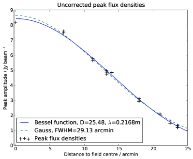
Figure 5: Peak flux densities of 3C 84 before and after primary beam correction. Left panel: Peak amplitudes measured using the pointings in Fig. 4 as a function of distance to the true source position. Also shown are two fits to the data, one using a Gaussian (dashed line) and one using an Airy disk (solid line). The Airy disk performs slightly better. Right panel: Peak amplitudes after applying the primary beam corrections using an Airy disk model fitted to the data in the left panel. The standard deviation of the measurements, normalised to their mean (shown as the solid line), is 0.039.

Since the receivers of the VLBA antennas are not aligned with the optical axis of the system, but are mounted off-axis, the beam patterns for the two orthogonal polarisations are offset on the sky by approximately 5 % of the primary beam FWHM (see Uson & Cotton 2008 and references therein for a detailed assessment of the effect at the VLA, which has similar antennas). This effect is called beam squint, and it needs to be taken care of in particular when measuring circular polarisation. In total intensity, however, the impact of beam squint is rather small, since RCP and LCP tend to average out. Nevertheless it was incorporated into the correction scheme here, using measurements of the squint carried out by R. Craig Walker (priv. comm., Tab. 3). These measurements were carried out at 1438 MHz, a few percent above the observing frequency used here. But beam squint is expected to be a fixed fraction of the primary beam width, and therefore the squint measurements were scaled linearly to the centre frequencies of the IFs used in our observations.

Table 3: Beam squint parameters at 1.438 GHz for the VLBA antennas (C. Walker, priv. comm.) The squint is angular separation of the RCP and LCP beams on the sky. The antennas are pointed towards the mid-point of the line connecting the two beams.

Antenna	Squint(R-L) Az	Squint(R-L) El
	arcmin	arcmin
St. Croix	$-1.53$	$-0.56$
Hancock	$-1.35$	$-0.67$
North Liberty	$-1.56$	$-0.62$
Fort Davis	$-1.56$	$-0.58$
Los Alamos	$-1.62$	$-0.67$
Pie Town	$-1.59$	$-0.63$
Kitt Peak	$-1.61$	$-0.59$
Owens Valley	$-1.76$	$-0.95$
Brewster	$-1.44$	$-0.50$
Mauna Kea	$-1.56$	$-0.60$

The results of the improved primary beam correction scheme can be summarised as follows. After applying the corrections to the data, the quality of the corrections was measured as the standard deviation of the corrected peak flux densities, normalised to the average peak flux density of the images from all pointings. This value was found to be 0.039, which is better than estimated by Middelberg et al. (2011a), and comparable to the typical amplitude calibration error assigned to VLBI observations (Figs. 5 and 6). The squint correction can be illustrated by plotting the ratio of the RCP and LCP amplitudes (Fig. 7). Overall the measurements indicate that the primary beam correction scheme performs well and does not introduce significant systematic errors.

Figure 6: Visibility amplitudes before and after primary beam correction. Left panel: Visibility amplitudes from all pointings on a few selected baselines before primary beam correction. The pointing centres are indicated at the bottom of the diagram. Shown is total intensity after averaging all frequencies and the two polarisations. Right panel: The same visibilities after primary beam correction. Whilst there are only small steps and discontinuities in the corrected visibilities (indicating that the correction scheme is working well), there are longer-term trends in the amplitudes, which may be attributed to the substantial structure of 3C 84, which was not modelled due to the poor $(u,v)$ coverage of the data. The larger scatter during some pointings is a consequence of the reduced sensitivity towards directions well away from the pointing centre.

Figure 7: Illustration of the effects of beam squint and its correction. Left panel: The ratio of the RCP and LCP amplitudes on a few selected baselines before primary beam correction. The pointing centres are indicated at the bottom of the diagram. Deviations from unity are caused by the RCP and LCP beams pointed at different positions. Right panel: The same visibilities after primary beam correction. The differences have essentially be eliminated.

3.5 Amplitude consistency between epochs

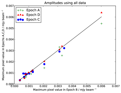
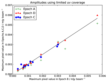
Figure 8: Illustration of the amplitude consistency between epochs. Left panel: amplitudes of a sample of bright sources in epochs A/C/D as a function of the amplitude in epoch B. Right panel: the same diagram but amplitudes have been extracted from images with the same limited $(u,v)$ coverage.

The amplitude errors can be estimated by imaging the data of a few bright sources from each epoch separately, and comparing the amplitudes between epochs. While this approach is susceptible to variability, however, selecting a sufficient number of sources (we use 18) is likely to be a robust estimator for the average amplitude error. Of this sample, 7 sources have been observed in two epochs only (e.g., in the overlap region between A/B, or B/C), 5 have been observed in three epochs (e.g., in A/D/B) and 6 in all four epochs. All sources were observed in epoch B (the one between A/D and C, see Fig. 1) to maximise the overlap. The brightest image pixel was extracted as a measure for the amplitude. All amplitudes from epochs A/C/D were then plotted against the amplitudes measured in epoch B (Fig. 8). The consistency of the amplitude calibration can be determined by calculating the median of the ratios of the amplitudes between epochs, and the standard deviation is a measure of the uncertainty when measuring individual flux densities (including the effects of variability). The median ratios of flux densities in the pairs A/B, C/B, and D/B were found to be 0.799, 0.955, and 0.990, respectively, and the standard deviations (i.e., errors for single measurements) were 0.100, 0.129, and 0.084. Epochs B/C/D therefore appear to be consistent within 1 $\sigma$, whereas epoch A deviates by around 20 %. One potential cause of this is the limited $(u,v)$ coverage during epoch A (where half the data were lost post-correlation due to a software bug). The exercise was therefore repeated by limiting the $(u,v)$ coverage in all epochs to the same extent, but the amplitude ratios and standard deviations were found not to have changed by much: the medians were determined for A/B, C/B, and D/B as 0.838, 0.989, 1.051, and the standard deviations 0.137, 0.143, and 0.078, respectively. Hence epoch A appears to yield consistently lower amplitudes by around 15 % to 20 %. However, epoch A contributed only 6 h of observing time out of a total of 42 h, therefore its contribution to the final sensitivity is only around 8 %, and the final images will only marginally be affected by this systematic error.

From this exercise one can conclude that the scatter of amplitudes between epochs arising from amplitude calibration errors, combined with potential source variability, is of order 10 %. This margin was used later in source extraction to determine the errors of the integrated flux densities.

4 Imaging and image analysis

Three types of images were made: naturally-weighted, untapered images, naturally-weighted images using a 10 M$\lambda$ taper, and uniformly-weighted, untapered images. Natural weighting was used for source detection, whereas uniform weighting was used to measure integrated flux densities.

An illustration of the sensitivity across the observed area is shown in Fig. 9. The measured rms fluctuations in the naturally-weighted images were placed on a regular grid and then linearly interpolated to the empty regions. The most sensitive region is slightly displaced from the centre of the field because the pointing at the north-east corner was observed twice, in epoch A and epoch D.

Natural weighting with no tapering was used to maximise the sensitivity to search for emission. It was expected that in some cases the VLA position was significantly offset from the VLBA core (because the VLA emission is extended and therefore potentially offset from the AGN), hence large images were made, covering 67.1 arcsec². The pixel size for these images was 1 mas, and the median resolution was 11.7$\times$9.4 mas². Deconvolution using the CLEAN algorithm was stopped after the first negative model component.

Additionally, tapered images were made using a Gaussian taper falling to 30 % at 10 M$\lambda$. This allowed to increase the pixel size to 2.5 mas to cover a larger area, at the expense of a 25 % increase of the image noise. Imaging a larger area was desirable for a small number of targets where the catalogued VLA position was significantly offset from the likely location of the nucleus. The median resolution was 21.7$\times$19.9 mas².

Finally, the data of detected sources were imaged using uniform weighting. In natural weighting, the distribution of the VLBA antennas causes the point spread function (the “dirty beam”) to exhibit a significant plateau around the main peak, as illustrated in Fig. 10. This plateau was found to increase the integrated flux density measurements, in particular at low SNR. Whilst deconvolution using the CLEAN algorithm in principle should separate the true emission from the dirty beam, we explored a variety of CLEANed images, and remains of the plateau were found in all. It was therefore decided that measurements of integrated flux densities were to use uniformly-weighted images, which do not exhibit similar artifacts. The pixel size for these images was 0.5 mas, and the median resolution was 7.4$\times$5.5 mas².

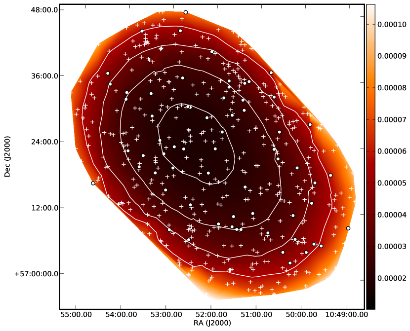
Figure 9: Sensitivity map of the VLBA observations. The rms noise of the individual images has been placed on a grid and then linearly interpolated to fill the map. The colour bar indicates Jy, and contours were drawn at $20\times\sqrt{2}^{n}\,{\rm\mu Jy/beam}$, $n=0...3$.

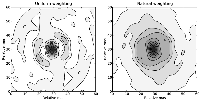
Figure 10: Point spread functions using uniform (left panel) and natural (right panel) weighting. Contours are drawn at 10 %$\times N$ ($N$=0, 1, 2, …, 9) of the peak. The plateau in the naturally-weighted image at the 30 % level is obvious.

4.1 Identifying detections

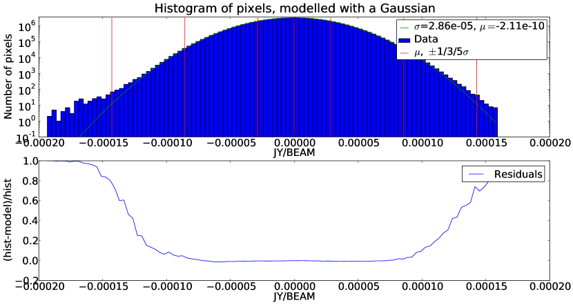
Figure 11: Histogram of the pixels in the image made from source L0211, which was not detected. The upper panel shows the histogram along with a model distribution calculated from the pixel’s $\sigma$, and vertical lines indicating the mean and $\pm 1\,\sigma$, $\pm 3\,\sigma$, and $\pm 5\,\sigma.$ The lower panel shows the residuals, normalised to the histogram. At the very low and very high end an excess of pixels can be clearly seen.

A common practice in radio surveys is to treat pixels exceeding 5 times the local noise as a detection. Since the images are relatively large, however, there is a substantial chance of having random noise peaks exceeding this threshold. We estimate this chance as follows.

The number of independent resolution elements, $N$, can be estimated following Eq. 3 in Hales et al. (2012):

$$N=\frac{A\times\bar{d}}{\Omega_{\rm b}},$$ (3)

where A is the covered area, $\bar{d}=\pi\sqrt{12}$ is a correction factor for the packing of the beams, and $\Omega_{\rm b}$ is the beam volume according to

$$\Omega_{\rm b}=\frac{\pi}{4{\rm ln}2}\Theta_{\rm maj}\Theta_{\rm min},$$ (4)

with $\Theta_{\rm maj}$ and $\Theta_{\rm min}$ the beam’s major and minor axes. Therefore, in this case here, with $A=8.192^{2}\,{\rm arcsec}^{2}=67.1\,{\rm arcsec}^{2}$:

$$N=\frac{67.1\,{\rm arcsec}^{2}\times\bar{d}}{\frac{\pi}{4{\rm ln}2}10\,{\rm mas}\times 8\,{\rm mas}}=671405.$$ (5)

If the image noise is Gaussian, the number of beams exceeding $5\,\sigma$, with $\sigma$ the standard deviation of the image pixels, is

$$N_{+5}=N\times[1-{\rm erf}(5/\sqrt{2})]/2=0.193.$$ (6)

However, it was found that $N_{+5}$ was of the order of 1 to 3 and sometimes was as high as 6. A typical pixel histogram clearly shows that the distribution of pixel values is non-Gaussian at the edges (Fig. 11). Exploring a number of different weighting schemes of the visibilities did not result in a reduction of the effect. Furthermore, averaging all images, to investigate whether the effect is a subtle structure present in all images, also did not result in conclusive evidence. The cause of this effect therefore remains unknown.

An unwelcome consequence of this is that the presence of a $5\,\sigma$ peak in an image is inadequate for deciding if a source has been detected or not, and a $6\,\sigma$ threshold had to be used for identifying true emission.

In five cases, $>6\,\sigma$ peaks were detected but deemed to be noise spikes since there was no coincidence with the VLA emission. Conversely, one has to conclude that a small number of the $>6\,\sigma$ detections which coincide with VLA emission potentially are chance coincidences. This fraction can be estimated as follows.

The median of the separation between the VLBA-detected emission and the maximum of the VLA emission is 133 mas, and in 88 % of the cases the separation was smaller than 500 mas (and in those cases where the separation was larger it was quite obvious that the VLA position was not a good indicator of the AGN position anyway). The area covered by a circle of 500 mas radius is only 1.2 % of that in an image which is 8.2 arcsec on a side. If one assumes that the number of $>6\,\sigma$ peaks is of order 10, and if these noise spikes are scattered randomly across the images, then the number of 6 $\sigma$ noise spike within 500 mas of the VLA position is, following a binomial distribution:

$$B(k=1|p=0.012;n=10)={n\choose k}p^{k}(1-p)^{n-k}=0.11,$$ (7)

i.e., less than 1. Since the number of random $>6\,\sigma$ noise peaks is likely to be smaller and visual inspection of images helps to weed out chance coincidences, one can be reasonably certain that no $>6\,\sigma$ peak coincident with a VLA and SWIRE source is due to noise.

4.2 Synthesis with VLA and SWIRE data

For a visual inspection of each of the 496 targeted sources, plots were generated to show a contour plot of the VLA emission superimposed on the 3.6 $\mu$m image from the SWIRE survey (Fig. 12). The SWIRE data from data release 3 were retrieved from the NASA/IPAC Infrared Science Archive and mosaiced using the Montage package, and then a 30”$\times$30” cutout centred on each VLA position was extracted. Postage stamps from the VLA observations were provided by Ibar et al. (2009). Contours were drawn from the $2\,\sigma$ level, to accentuate faint emission, increasing by factors of 2. The two VLBA images for each source – untapered and tapered – were analysed and searched for emission. Along with these data a contour plot was produced of the untapered VLBA image, centred on the brightest image pixel, starting at $2\,\sigma$ and increasing by factors of two. These plots were used to group catalogued radio components to radio sources, to identify the correct SWIRE counterparts to these sources and to check the plausibility of a VLBA detection. The three sources shown in Fig. 12 illustrate this process.

As was noted in Sect. 1.1 and is further discussed in Sect. 5, only sources with an integrated VLA flux density exceeding 6 times the noise in the VLBA images were deemed to be detectable, and after calibration only 217 sources were found to satisfy this criterion. Nevertheless, we inspected all 496 targeted sources, to ensure proper cross-identifications and to inspect the data for errors (such as the false $>6\,\sigma$ peaks described in Sect. 4.1) and unexpected results. However, none of the remaining $(496-217)=279$ sources with insufficient sensitivity in the VLBA data were found to yield a credible VLBA detection.

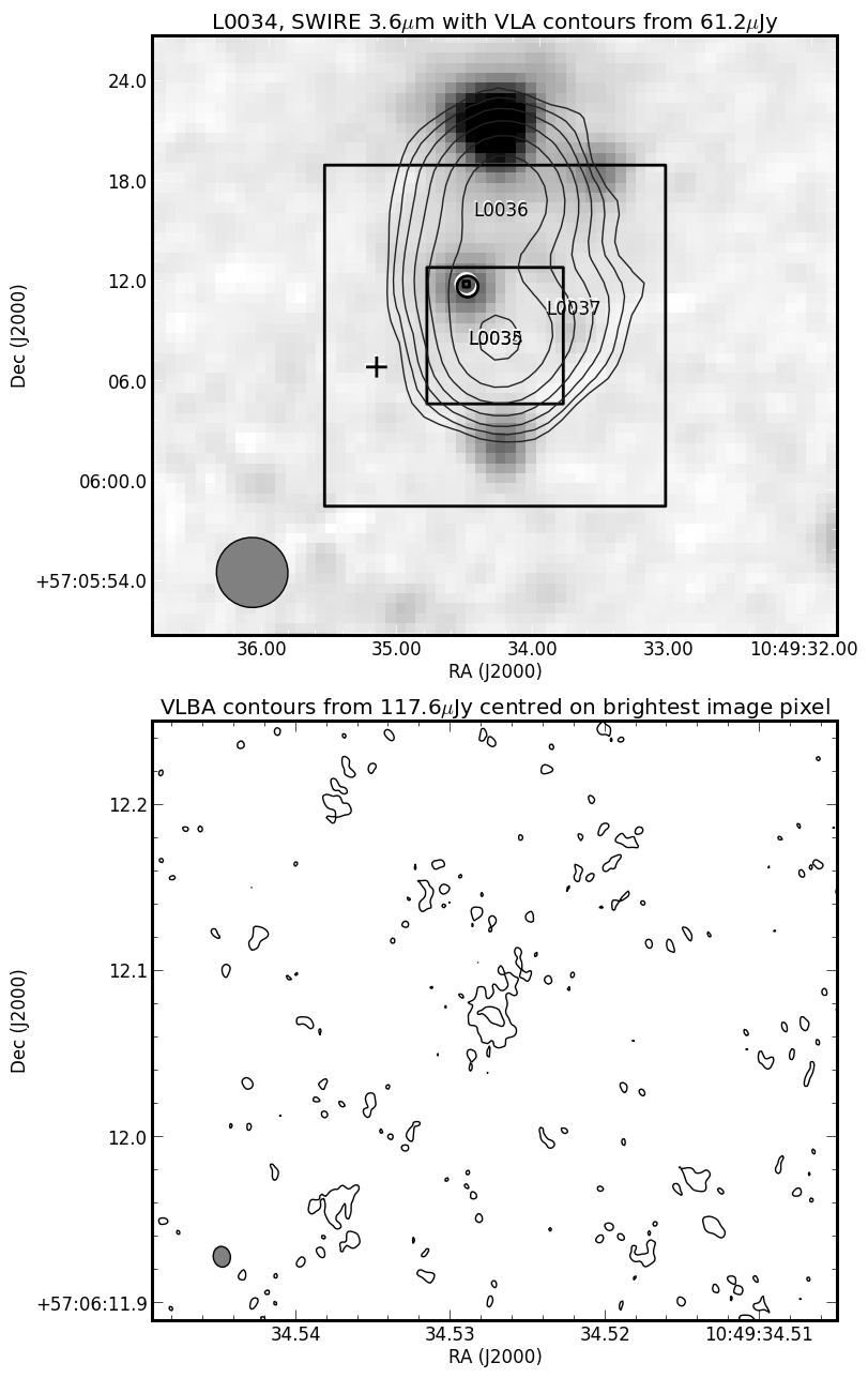
(a)

Figure 12: Example contour plots of the VLBA, VLA, and SWIRE data. The upper panel shows the logarithm of the SWIRE 3.6 $\mu$m emission as a pixel map, superimposed with contours of the VLA data of source L0034. Contours start at 2 times the local rms (as indicated in the plots) and increase by factors of 2. This object has four entries in the VLA catalogue: one, L0034, representing it as a source and three for its constituents, L0035, L0036, and L0037. Their locations are marked as labels in the image. Three black squares indicate (from large to small) (i) the regions imaged with the VLBA using a 10 M$\lambda$ taper, (ii) the region imaged using untapered data, and (iii) the region shown in the contour plot in the bottom panel. The maximum of the tapered VLBA data is marked with a cross, and the maximum of the untapered VLBA data is marked with an open circle. In this case, the maxima of the tapered and untapered VLBA images are not coincident, because the tapered image has reduced sensitivity. However, the maximum of the full-resolution (6.2 $\sigma$) coincides with a faint SWIRE source located between L0035 and L0036, indicating that this is the location of the AGN. Furthermore, the value of the tapered image exceeds $5\,\sigma$ at the location of the maximum of the untapered image, adding credibility to the detection. The bottom panel shows a contour map of a region 0.36 arcsec across, centred on the maximum of the untapered VLBA image. Contours start at 2 times the local rms (as indicated in the plots) and increase by factors of 2.

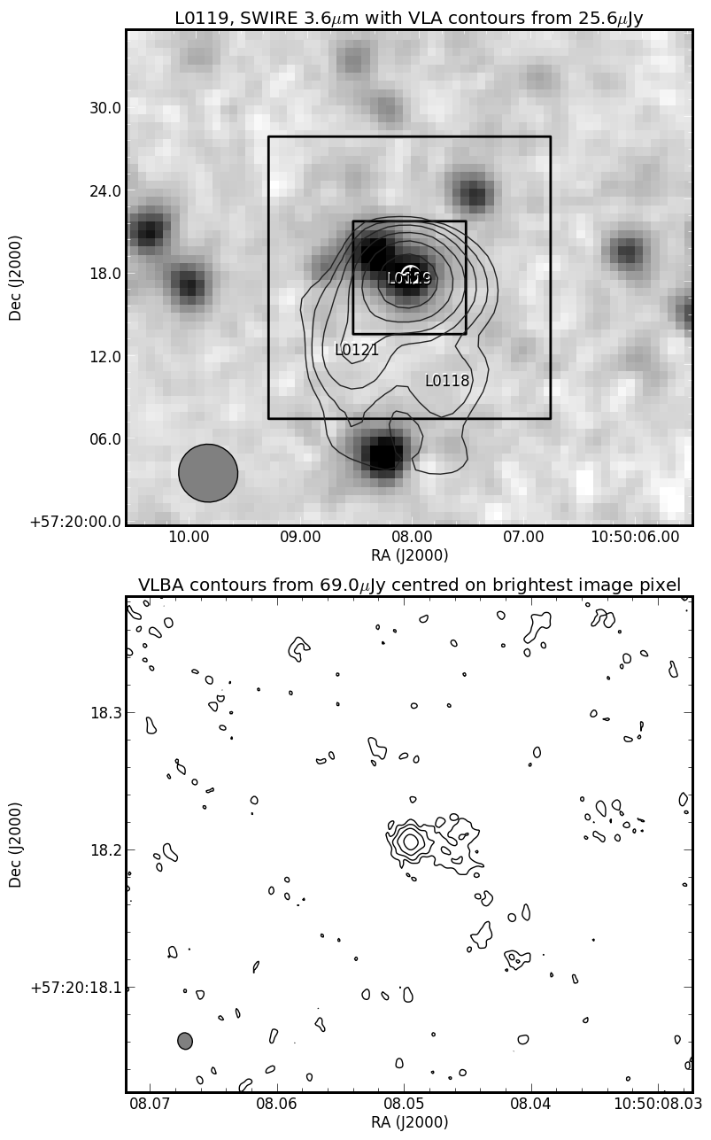
(b)

Figure 12: (continued) This plot shows data for source L0119. Three catalogued VLA components belong to this source. The detection at 24 $\sigma$ and cross-identification with a SWIRE source is unambiguous.

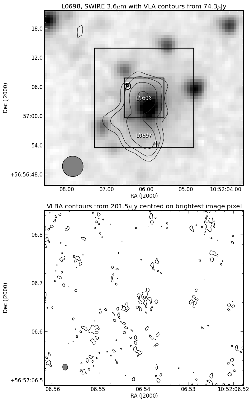
(c)

Figure 12: (continued) This plot shows data for source L0698, which has been grouped with source L0697. The maxima of the two VLBA images do neither coincide with one another, nor with an infrared source, and therefore this source with a maximum of 5.2 $\sigma$ was deemed to be undetected.

4.3 Flux density extraction

In radio astronomy, source flux densities are commonly measured using models of 2D Gaussians to the image pixels. Whilst this method is suitable under well-constrained circumstances, it is known to yield inaccurate results when left unconstrained. For example, if the SNR of a source is below 10, then a 2D Gaussian is likely to overestimate the flux density. Also if a source has a non-Gaussian shape then the model is inappropriate and will yield incorrect results. In a recent publication, Hales et al. (2012) presented a source extraction program, BLOBCAT, which uses the flood fill algorithm to measure the integrated flux density of sources. It takes proper account of the various biases involved and performs better than Gaussian fits when the source has low SNR or is irregularly shaped. It was therefore used to measure the flux densities of the VLBA-detected sources from uniformly-weighted images.

Two modifications to the default settings of BLOBCAT were made. First, a pixellation error of only 1 % was assumed because of the significant oversampling of the point spread function (--ppe=0.01). Second, the error of the surface brightness in the images was assumed to be 10 % (--pasbe=0.1), reflecting the amplitude calibration errors.

5 Discussion

The most basic result from the VLBA observations of the Lockman Hole/XMM is whether or not a source is detected, and what its flux density and morphology are on mas scales. Even though the initial sample consisted of 496 radio sources with $S>100\,\mu$Jy it was always clear that many would not be detectable with our observations, because the VLA had a $1\,\sigma$ sensitivity of $6\,\mu{\rm Jy\,beam^{-1}}$, compared to a $1\,\sigma$ sensitivity of just under $20\,\mu{\rm Jy\,beam^{-1}}$ of our VLBA data. For the subsequent analysis a sub-sample was selected based on whether sources would have been, in principle, detectable. The criterion we used was that the noise in the full-resolution, naturally-weighted image was smaller than 1/6 of the VLA peak flux density, because we used a 6 $\sigma$ threshold for source detection. Out of the original sample, 217 sources satisfied this criterion and were used for analysis. Out of these 217 detectable sources, 65 were deemed to be actually detected. Note that whilst naturally-weighted images were used to determine detections because of the higher sensitivity, flux densities were measured from uniformly-weighted images to reduce the effect of the plateau in the point spread function (see Sect. 4 and Fig. 10).

5.1 Fraction of detected sources

The fraction of VLBA-detected sources is an interesting quantity because it essentially gives us a lower limit on the number of radio-emitting AGN in the sample. Since our sample is large we can subdivide it and determine the detection fraction as a function of flux density. The results are shown in Fig. 13 and Table 4.

The fraction of VLBA-detected sources is obviously a function of sensitivity. Towards faint flux density levels only sources which are increasingly compact can be detected, yet at some flux density level the detection fraction approaches completeness. One can estimate that level as follows. Around 90 % of the targets have been observed with a sensitivity of 60 $\mu$Jy/beam^-1, allowing the detection of sources brighter than 360 $\mu$Jy, when a $6\,\sigma$ cutoff is used. If one requires a minimum of 10 % of that flux density to come from the core, providing emission for a VLBA detection, then sources brighter than 3.6 mJy can be detected across 90 % of the area. In Fig. 13 (right panel), the nearest point is at 3.2 mJy, and the detection fraction is 60 % (12 out of 20 sources).

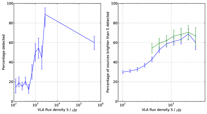
Figure 13: Fraction of VLBA-detected sources. Left panel: The fraction of VLBA-detected sources as a function of flux density. Detectable sources have been grouped into bins with limits 100 $\mu$Jy$\times\sqrt{2}^{N}$, $N=0,1,2,...$. Error bars denote the 68 % confidence interval for a small-sample binomial distribution, according to Clopper & Pearson (1934). Whilst at the faintest flux density levels only around 15 % have been detected, this fraction rises sharply at a level of around 0.5 mJy, and increases to more than 80 % at the 2 mJy level. Right panel: Using the same bins as for the left panel, the fraction of detected sources brighter than the bin limits has been calculated. Whilst of all sources brighter than 100 $\mu$Jy 30 % have been detected, the fraction reaches 60 % when all sources brighter than 1 mJy are considered. The green line indicates the data of the CDFS from Middelberg et al. (2011a), which had a maximum sensitivity of $55\,\mu{\rm Jy/beam}$, compared to just under $20\,\mu{\rm Jy/beam}$ in our data. All curves are subject to small number statistics, which causes the Lockman Hole data to drop at the bright end and the discrepancy between the CDFS and Lockman Hole data.

Table 4: Fraction of detected sources as a function of VLA flux density.

Bin edges	$N_{\rm VLA}$	$N_{\rm detected}$	%
$\mu$Jy
100.0- 141.4	14	2	14
141.4- 200.0	26	5	19
200.0- 282.8	33	5	15
282.8- 400.0	39	8	21
400.0- 565.6	25	3	12
565.6- 800.0	17	5	29
800.0- 1131.3	14	7	50
1131.3- 1600.0	11	6	54
1600.0- 2262.7	9	4	44
2262.7- 3200.0	9	8	89
$>$3200.0	20	12	60.0

5.2 Variability

For an unresolved radio source, the interferometric visibility amplitude is constant with baseline length; for resolved sources, it must generally decrease with baseline length (although constructive interference between separated, compact components can lead to local increases). When comparing VLBA baselines with lengths of hundreds to thousands of kilometres to VLA baselines with lengths of much less than 100 km, it can be safely assumed that the visibility amplitudes on longer baselines must be less than, or at most equal to, the visibility amplitudes on short baselines.

It is therefore a useful consistency check to compare the VLBA flux densities to the VLA flux densities. In Fig. 14 the ratios of the integrated VLBA peak and integrated flux densities to the integrated VLA flux densities are plotted for all detectable sources and the 65 detected ones. Out of the 65 detected targets, 6 have ratios which exceed 1.0 by more than the width of their error bars ($1\,\sigma$), in particular at low flux densities: L0231, L0578, L0593, L0648, L0997, and L1200. While it is clear that some sources might have flux density ratios in excess of $1+\sigma$, one source (L0593) exceeds $1+3\,\sigma$, which is significant given our sample size. We interpret this result as source variability, for several reasons:

• Although the variability of bright radio sources has long been studied, the variability of the mJy and sub-mJy radio source population is poorly constrained. Carilli et al. (2003) found that the density of variable sources in this flux density regime is less than $5\times 10^{-3}\,{\rm arcmin}^{-2}$.

• The elapsed time between the VLA and VLBA observations is significant. Whilst the VLBA observations where carried out in July-September 2010, the VLA data were obtained between 2002 and 2005.

• Faint sources are preferably detected if they are variable and in a state with high flux density, compared to their average flux density. Faint sources in a state with low flux density will be missed, and this is the reason why the fraction of sources with ratios greater than 1 increases towards fainter flux densities.

• The VLA observations are sensitive to the combined emission from star formation and AGN, whereas the VLBA observations isolate the AGN emission. Hence the variability of the AGN is likely to be higher than determined by our observations, because only one of our two available flux density measurements (VLA and VLBA) is purely sensitive to the AGN emission.

The effect of interstellar scintillation on the source flux densities is difficult to estimate with our data, but is likely to be small. The galactic latitude of the Lockman Hole/XMM field is $53^{\circ}$, where, according to Walker (1998), sources (or parts thereof) are required to be smaller than around $6\,\mu$as (0.05 pc at $z=1$) to show significant scintillation. Most of the VLBA-measured flux densities are lower than the VLA flux densities, implying that the sources are partly resolved between the length scales probed by the VLBA and VLA. We deem it safe to assume that most, if not all, of the sources had been resolved further, had the resolution of our observations been higher. Thus, whilst it is possible that small fractions of the flux density recovered by our VLBA observations originate in regions sufficiently small for scintillation, we do not expect it to have a significant effect.

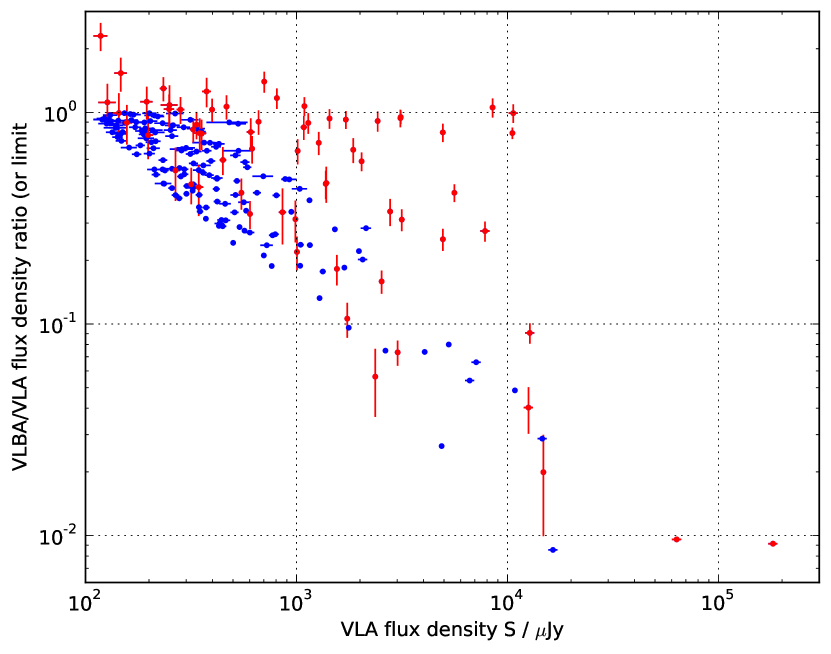
Figure 14: Ratio of the VLBA and VLA flux densities. Blue dots show the detectable sources, placed at $6\times{\rm rms}/S_{\rm VLA}$ (where rms is the local noise level of the VLBA observations), and red dots with error bars detected sources. Out of the 65 detected sources, 6 exceed a ratio of 1.0 by more than 1 $\sigma$, but only one source exceeds $1+3\,\sigma$.

5.3 Spectral index

A common method to classify radio sources into AGN and non-AGN is to use the spectral index, $\alpha$, with $S\propto\nu^{\alpha}$. Sources with spectral indices of more than $-0.3$ (“flat” or “inverted”) or less than around $-1.0$ (“steep”) are typically classified as AGN, because flat and inverted spectral indices arise in compact, optically thick synchrotron emitters typical of AGN, whereas steep indices are attributed to optically thin emission from radio lobes, with a potentially aged particle population. Sources with $\alpha$ around $-0.7$ can not be classified based on spectral index alone, because both starburst galaxies and AGN can exhibit such values, which arises from synchrotron emission with a continuous injection of fresh particles (e.g., Pacholczyk 1970).

Whilst the histogram of the spectral indices of detectable sources is typical of the population found in sensitive, extragalactic radio surveys, the histogram of detected sources exhibits a prominent deficiency at low spectral indices. The lowest spectral index of any detected source is $-0.88$, whereas the distribution of detectable sources extends to well below $-1.0$. Almost all sources with $\alpha>0.0$ are detected, but no source with $\alpha<-0.9$ is.

One might argue that this is a selection effect, which de-selects steep spectral indices, because they tend to have lower 1.4 GHz flux densities than flat- or inverted-spectrum sources (the spectral indices at our disposal were measured between 610 MHz and 1.4 GHz). However, we find only a mild correlation between the spectral index and the flux density, with a product-moment correlation coefficient of $-0.02$ (where $+1$ and $-1$ denote perfect linear correlation and anti-correlation). We therefore conclude that, whilst inverted spectra arise from compact synchrotron emission and therefore are likely to be detected, steep spectral indices arise from larger and therefore potentially older regions, which tend to be resolved out. What follows from this exercise is that at “normal” spectral indices of between $-1.0$ and $-0.3$ VLBI observations can cleanly separate the AGN from star-forming activity, whereas in the regime of $\alpha>-0.3$ spectral index alone is already a good indicator for AGN.

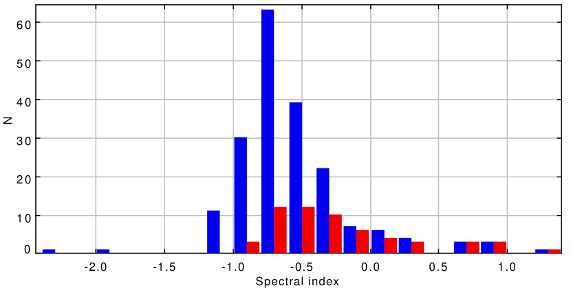
Figure 15: A histogram of the spectral indices of detectable (blue bars) and detected (red bars).

5.4 Source counts

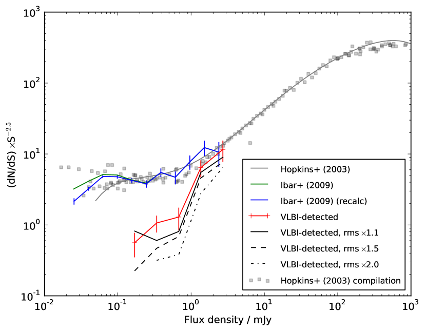
Figure 16: Source counts in the Lockman Hole/XMM field. Shown are the euclidean-normalised source counts of the VLBA-detected sources, using their VLA flux densities (red line). Shown with black lines are source counts which would have been measured had the sensitivity of our observations been lower by factors of 1.1, 1.5, and 2.0. For comparison, we have plotted the source counts constructed from the Ibar et al. (2009) data using the same methods (blue line), the source counts as published by Ibar et al. (2009) (green line), and the data compilation from Hopkins et al. (2003) (light grey squares) along with their 6th order polynomial fit.

While radio source counts of VLBI-detected sources at flux density levels of above 100 mJy are in principle available from VLBI calibrator searches, counts of the mJy and sub-mJy population are yet unknown, because they would have required prohibitive amounts of observing time using conventional methods. The work presented here yielded only the detection of 65 sources in total (a number frequently found in a single bin in other source count studies), yet this is, to our knowledge, the first attempt to produce radio source counts of VLBI-detected sources in the mJy and sub-mJy regime.

It is worth noting that in this paper we do not construct radio source counts using VLBI flux densities, since such measurements would be plagued by tremendous resolution effects which would render the source counts useless. Instead, we use the VLBI observations to select a sub-sample of radio sources with very compact cores from the parent sample of known radio sources detected with the VLA, and then use the VLA flux densities of this sample to construct the source counts.

When constructing source counts, two effects need to be taken into account. The first is a weighting factor arising from the varying sensitivity of the observations, i.e., each source flux density one needs to determine over which area this source would have been detected. Since observations typically have significantly smaller areas with very high sensitivity than with lower sensitivity, this correction can have a large effect on the source counts if not carried out correctly. The second effect is resolution bias. Extended sources can remain undetected when they are close to the detection limit of the survey, and so the counts at low flux density levels will underestimate the true source counts. This effect depends on the resolution of the observations, and in our case is much smaller than the correction for effective area, of order below 10 % (Ibar et al. 2009). Hence the number of sources in each bin needs to be corrected by $1+c$, where $c$ is of order 0 to 0.1.

As a consistency check, we initially constructed the source counts from the VLA data published by Ibar et al. (2009). From their catalogue we have eliminated all entries marked as components (non-zero “m_Name” column). Corrections for effective area and resolution were extracted from their Figs. 6 and 7, from which we constructed look-up tables using Dexter. Using the same bins as Ibar et al. (2009) we determined

$$s=\sum_{N}S/A_{\rm eff}$$ (8)

for the $N$ sources in each bin, where $A_{\rm eff}$ was determined from a look-up table. This procedure ensures proper weighting of all sources in a bin. Each bin was then corrected for resolution bias by multiplying its value by $1+c$, where $c$ is a value extracted from the other look-up table. The bin values were then divided by the bin widths, and subsequently by the geometric mean of the bin edges raised to the power of $-2.5$. Count errors of the area-weighted counts in Eq. 8 were estimated as $\sqrt{N}/N\times s$ and then propagated through the same steps as the counts themselves. This procedure resulted in identical counts as published by Ibar et al. (2009), with the exception of the two lowest bins, where we found agreement with previously published counts (Fig. 16). The reason for this discrepancy can in principle arise from the way the effective area is dealt with. If one uses, e.g., the lower edge of a bin to calculate the effective area for the entire bin, then one underestimates the area over which a source would be detected, resulting in an over-estimate of the source counts.

We proceeded to calculate the source counts for the VLBA-detected sources only, using the same methods as for the VLA source counts. However, the determination of the effective area was different. Two corrections are needed to properly account for the effective area – one to determine over which area each source would in principle be detectable with the VLBA, another to determine the area over which this source would in principle be detectable with the VLA. The first correction was carried out as follows. For each source the area over which it could have been detected with the VLBA was determined using the sensitivity map shown in Fig. 9. The number of pixels with values smaller than 6 times the VLA source flux density was counted and multiplied with the pixel area. The second correction would have required knowledge about the rms distribution of the VLA observations, which were not available (the catalogue of Ibar et al. 2009 only lists peak-to-noise ratio, but neither peak nor noise are given). However, Fig. 6 in Ibar et al. (2009) indicates that for our weakest source greater than the lowest bin edge at 120 $\mu$Jy, at $S=127\,\mu{\rm Jy}$, the area over which it was detectable is 94 % of the entire observed area, and for stronger sources this percentage comes even closer to 100 %. We therefore neglected this correction.

The source count bins were defined to begin at a total integrated flux density of 120 $\mu$Jy and to increase by a factor of two to 3.84 mJy. This resulted in a reasonably even distribution of the number of sources per bin. The source counts of all sources, the VLBA-detected sources, and the source counts by Hopkins et al. (2003) are shown in Fig. 16.

At the bright end of the distribution the source counts of VLBA-detected sources appear to be an extrapolation of the general radio source counts, indicating that this population is dominated by AGN. Between 1 mJy and 2 mJy there is a sharp drop, which is also visible in the percentage of detected sources in Fig. 13 (left panel). However, the counts of VLBA-detected sources exhibit a shoulder between 0.1 mJy and 1 mJy, and this shoulder is a lower limit on the number of radio-emitting AGN at sub-mJy flux density levels.

It is important to note here that this lower limit is subject to the resolution of the VLBA observations. At high flux densities a detection can be made even if only a small fraction of the radio flux density originates from the AGN, whereas at flux density levels near the detection limit only the most compact sources will be detected (see Fig. 14). Our counts near the VLBA detection limit therefore underestimate the “true” detection rate by a larger margin than at higher flux density levels. At higher sensitivity, the counts of VLBA-detected sources would rise towards the general radio source counts.

To illustrate this effect we have constructed source counts which would have been measured with lower sensitivity. We multiplied the sensitivity map in Fig. 9 by factors of 1.1, 1.5, and 2.0 and selected only those sources which would have been detected with this increased noise level. This was done by selecting sources with a peak flux density in the VLBA observations of 6 times the modified noise. The source counts from this exercise are shown in Fig. 16 as black lines (solid, dashed, and dash-dotted). One can see that the source counts drop with decreasing sensitivity, as expected, because less sensitivity requires that only the most compact sources can be detected. Conversely, if one extrapolates this trend to higher sensitivity, one can conclude that the source counts of VLBA-detected sources are likely to be higher, above the red line, but below the general radio source counts.

We therefore conclude that at flux density levels of between 0.1 mJy and 1 mJy, at least 15 % to 25 % of the radio sources contain radio-emitting AGN. This finding adds new and independent support for the recently established picture that a substantial fraction of the sub-mJy radio populations is AGN-driven, rather than powered by star-forming activity. For example, Smolčić et al. (2008) classified radio sources from the COSMOS survey using optical colours and found that 50 % to 60 % of the sub-mJy radio sources contain AGN. In another study, Padovani et al. (2011) classified radio sources in the Chandra Deep Field South using Spitzer data, and found that 50 % contained AGN. A recent compilation of studies investigating the AGN fraction of the sub-mJy radio source population can be found in Fig. 4 of Norris et al. (2011b).

Table 5: Source counts of VLBA-detected sources.

Bin edges	$\langle S\rangle$	$N$	$dN/dS$	$(dN/dS)S^{-2.5}$
$\mu$Jy	$\mu$Jy		Jy-1 sterad-1	Jy1.5 sterad-1
120.0-240.0	169.7	7	1.50e+09	0.561$\pm$0.212
240.0-480.0	339.4	14	5.02e+08	1.066$\pm$0.285
480.0-960.0	678.8	8	1.08e+08	1.292$\pm$0.457
960.0-1920.0	1357.6	14	9.45e+07	6.419$\pm$1.716
1920.0-3840.0	2715.3	9	3.02e+07	11.589$\pm$3.863

5.5 The extended emission

As one can see in Fig. 14, the flux density recovered with the VLBA is in general a fraction of the VLA flux density. Variability can only explain a small fraction of this trend, but not the large differences found in many sources, nor the majority of the VLBA non-detections. Moreover, Fig. 15 shows that the spectral indices of the VLA sources (extended) tend to be lower than those of the VLBA sources (compact), indicating that the nature of the compact emission is different than that of the extended emission. Here, we assume that the compact emission comes from the AGN, whereas the extended emission comes from star-formation, either circumnuclear, or from the host galaxy. In a recent study of radio-quiet ($L\lesssim 10^{24.5}\,{\rm W\,Hz^{-1}}$) VLA sources in the Chandra Deep Field South (CDFS), Padovani et al. (2011) found that the bulk of the their emission comes from star-formation processes, by comparing the luminosity functions of radio-quiet AGN, radio-loud AGN and star-forming galaxies. Also Fig. 16 showed that the source counts of VLBA-detected and VLBA-undetected sources follow a dichotomy, so it is safe to assume that the extended part of the emission traces star-formation, whereas the compact emission traces the AGN.

A sample of AGN where we can measure the host galaxy properties (star-formation rate) independently from the AGN emission provides us with the opportunity to test the co-evolution of the AGN and their hosts. There is observational evidence that some co-evolution between the AGN and the host galaxy exists (e.g., the M-$\sigma$ relation, Ferrarese & Merritt 2000), and recent observations link host SFRs to their AGN for different luminosities and redshifts (see Shao et al. 2010; Mullaney et al. 2012; Rovilos et al. 2012; Rosario et al. 2012, but also Page et al. 2012). In Fig.17 we plot the difference between the VLA and the VLBA luminosities (see Sect. 5.6 and Tab. 7) as a function of VLBA luminosity for our sample. There are a number of sources for which the VLBA luminosity is higher than the VLA luminosity, and we assume that this is because of variability (see Sect. 5.2). These cases have been treated as follows: in cases where $L_{\rm VLA}+\Delta L_{\rm VLA}<L_{\rm VLBA}-\Delta L_{\rm VLBA}$, we assumed that the extended component of the radio emission seen by the VLA but resolved out by the VLBA was small. Since some extended emission is likely to be present, we adopted an upper limit of the extended component of 5 % of the VLA luminosity. In cases where $L_{\rm VLA}<L_{\rm VLBA}$ but $L_{\rm VLA}+\Delta L_{\rm VLA}>L_{\rm VLBA}-\Delta L_{\rm VLBA}$, we used $L_{\rm VLA}+\Delta L_{\rm VLA}-(L_{\rm VLBA}-\Delta L_{\rm VLBA})$ as an upper limit of the extended component.

One can see from Fig. 17 that there is a positive correlation between the two luminosities, and applying the generalised Kendall’s $\tau$ method using the ASURV package (Rev. 1.3, Lavalley et al. 1992), we find that the significance of the correlation is at the 96.2% level. The solid and dotted lines correspond to the equation:

$$\log\left(L_{\rm VLA}-L_{\rm VLBA}\right) =$$

$$(0.66 \pm 0.24)\log\left(L_{\rm VLBA}\right)+(7.2\pm 1.0)$$ (9)

(only the standard deviation of the normalisation is shown in the dotted lines). If we ignore the upper limits, the significance rises to 97%. However, one can also see that in a small number of sources the extended luminosity is larger than $\rm 10^{24.5}\,W\,Hz^{-1}$, so there might be a contribution from the AGN to the extended flux, from structures which are resolved out by the VLBA observations. Ignoring those cases, the correlation becomes even more statistically significant, at the 99.81 % and 99.98 % levels, including and excluding upper limits, respectively.

Figure 17: The difference between the 1.4 GHz radio luminosity measured with the VLA, $L_{\rm VLA}$ and measured with the VLBA, $L_{\rm VLBA}$, as a function of $L_{\rm VLBA}$. The solid line indicates the correlation as indicated in the text, and the dotted lines the error of the normalisation.

An issue that needs to be addressed is whether the correlation is driven by a redshift effect. It is known that the mean star-formation rate increases with redshift up to z$\approx$2 (see, e.g., Daddi et al. 2007; Elbaz et al. 2011), and also the VLBA luminosity can increase with redshift, because the survey is flux density-limited. Such an effect can mimic an AGN-host correlation (see Mullaney et al. 2012). As a test we determined the correlation in the flux density domain and found that after excluding the upper limits the correlation is at the 94.7 % level, but its significance drops to 91.8 % if we include the upper limits. We therefore claim that a tentative correlation exists. This tentative correlation shows that the most luminous VLBA AGN tend to have higher levels of star-forming activity and argues against quenching of the star-formation by AGN feedback when the AGN luminosity reaches a certain level (e.g., Page et al. 2012), at least for the case of compact radio AGN. This shows that the mechanical power from the AGN, which is detected at radio wavelengths, is not sufficient to disrupt the host galaxy and stop the star-formation, a process which may be attributed to radiation pressure (King 2005). On the contrary, radio AGN activity might even enhance the star-formation rate, by creating disruptions of the hosts’ density profiles (Gaibler et al. (2012)).

5.6 Multi-wavelength properties of the detected sources.

In addition to the basic results from the VLBA survey, significantly more information can be gathered from the literature, to obtain flux densities at other wavebands. Therefore the VLA and VLBA observations were cross-matched to the publicly available multi-band photometry and photometric redshift catalogues of the Lockman Hole/XMM by Fotopoulou et al. (2012). In this catalogue the Large Binocular Telescope (LBT) images presented in Rovilos et al. (2009) were combined to create a new catalogue of optically and near-infrared detected sources in the field. In addition to the $UBV$ bands this multi-wavelength photometry catalogue includes the PSF-homogenised fixed-aperture photometry from LBT $Y$ and $z$-band observations, the Subaru $R$, $I_{c}$, $z^{\prime}$ bands from Barris et al. (2004), the UKIDSS $J$ and $K$ bands, the 3.6 $\mu$m to 8.0 $\mu$m photometry from the Spitzer Wide-area Infrared Extragalactic survey (SWIRE, Lonsdale et al. 2003) and GALEX photometry. Except for the near-infrared data, all the other bands provide very sensitive data (see Table 2 of Fotopoulou et al. 2012 for the depth of the optical bands). The photometric redshift catalogue uses all the above-mentioned bands to produce accurate photometric redshifts for normal galaxies and for X-ray detected sources by using templates of normal galaxies and AGN hybrids, and luminosity and morphological priors to reduce the parameter space of possible redshift solutions (more details can be found in Fotopoulou et al. 2012).

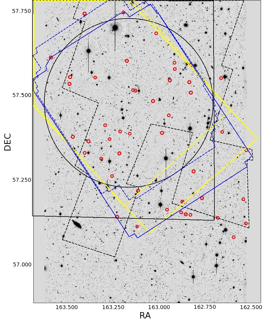
Figure 18: VLBA-detected sources with optical counterpart (red circles). The multi-wavelength coverage of the field is also shown: Subaru $R_{c}$, $I_{c}$, $z^{\prime}$ filters (image), LBT $U$ and $B$ filters (blue solid line), LBT $VYz^{\prime}$ filters (blue dashed line), IRAC 3.6 $\mu$m and 5.8 $\mu$m (yellow solid line), IRAC 4.5 $\mu$m and 8 $\mu$m (yellow dashed line), SDSS (black dashed line), $J$ and $K$ UKIDSS filters (black solid lines). The black circle denotes the area observed by XMM-Netwon.

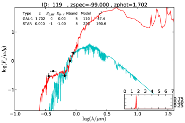
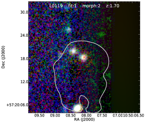
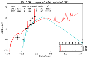
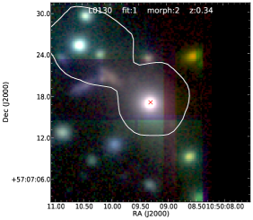
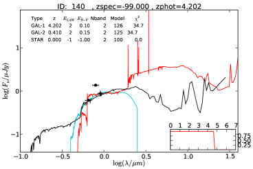
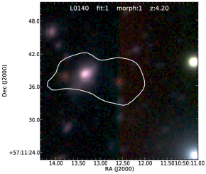
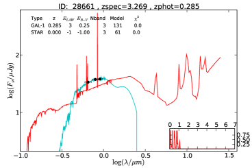
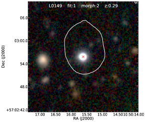
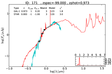
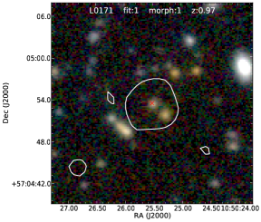
Figure 22: Left column: UV to mid-infrared SED fits. Black points: photometric observations, red line: best-fitting model, cyan line: stellar template, black line (where applicable): galaxy template of second photometric redshift solution. The inset shows the probability distribution function of the best-fit model. right column: RGB cutouts made from Subaru $R_{c}I_{c}z^{\prime}$ images, with a single VLA contour overlaid and the VLBA position indicated with red crosses. These images show regions 28.8 arcsec$\times$28.8 arcsec in size.

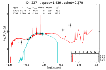
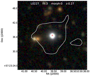
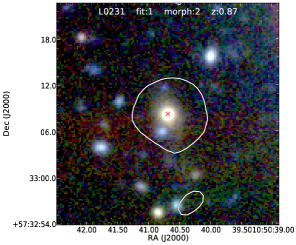
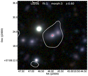
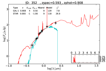
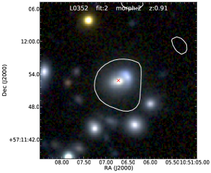
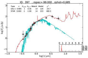
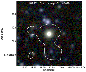
Figure 22: (Continued)

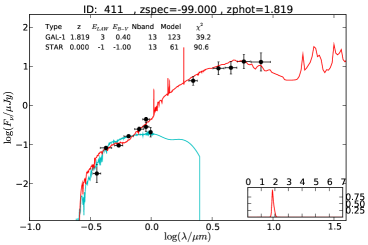
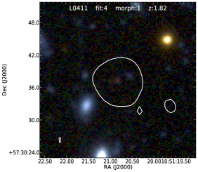
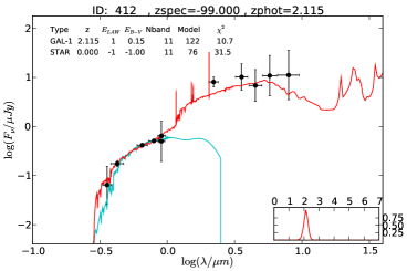
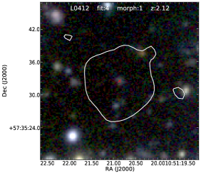
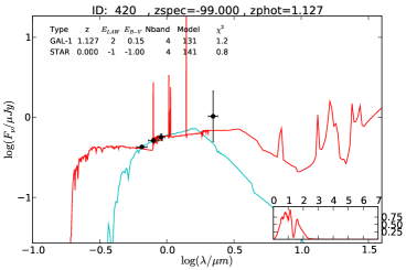
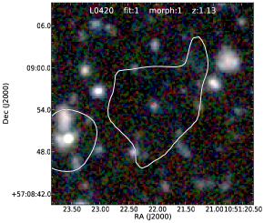
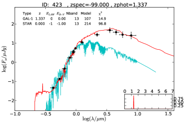
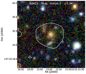
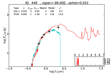
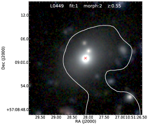
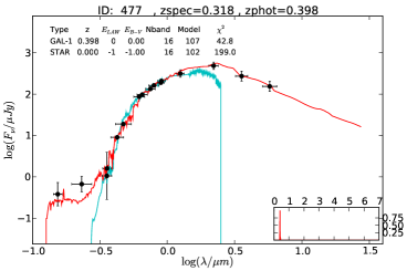
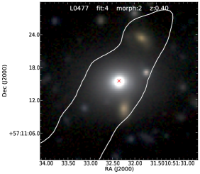
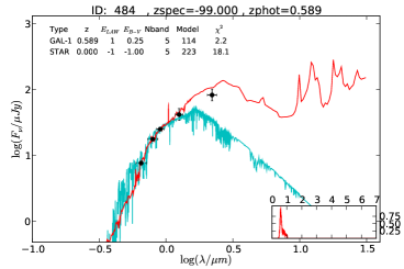
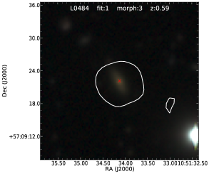
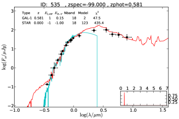
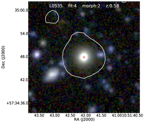
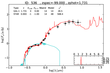
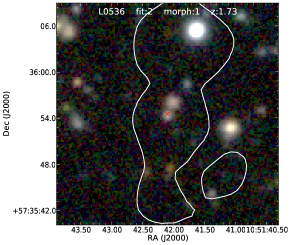
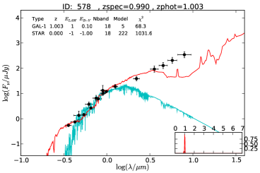
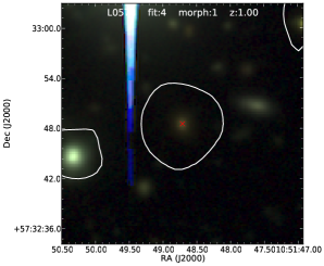
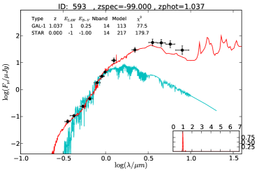
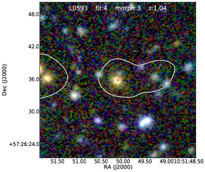
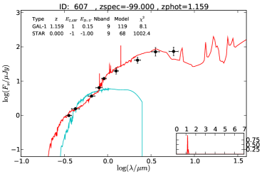
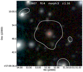
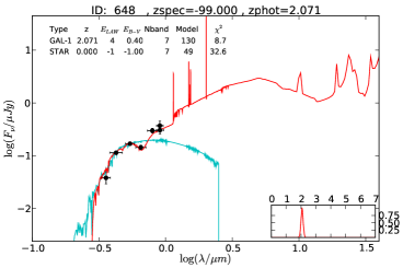
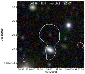
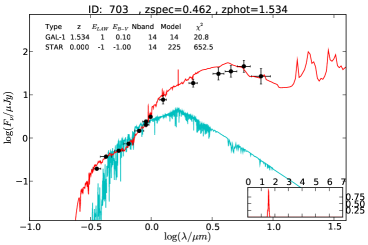
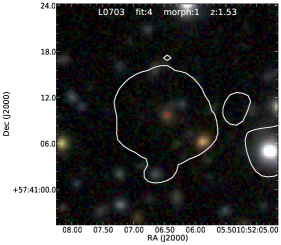
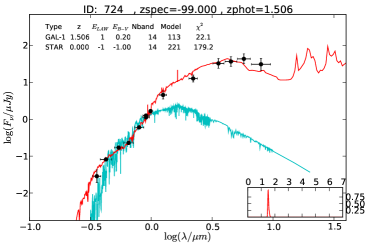
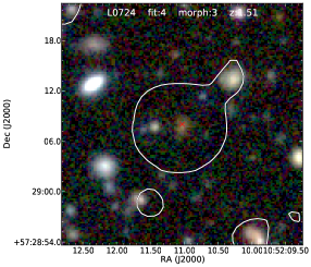
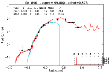
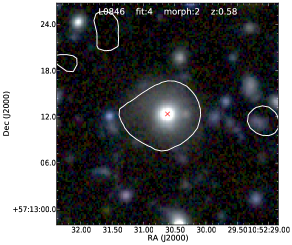
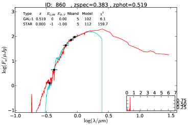
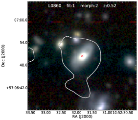
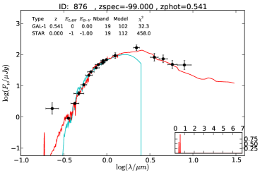
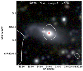
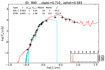
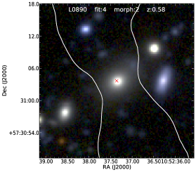
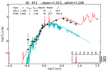
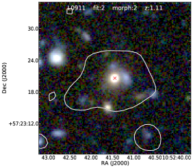
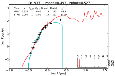
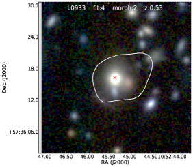
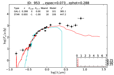
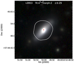
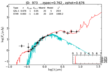
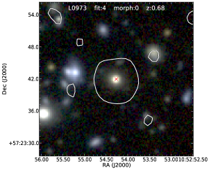
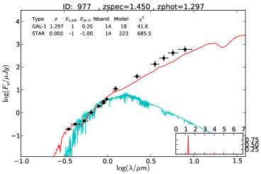
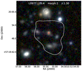
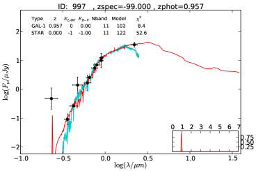
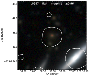
Figure 22: (Continued)

Figure 22: (Continued)

Figure 22: (Continued)

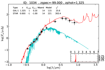
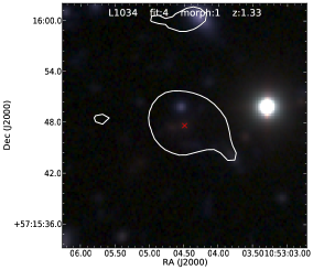
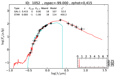
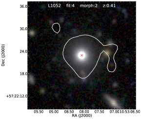
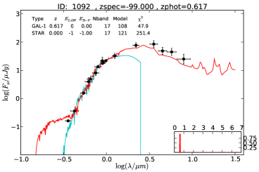
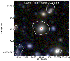
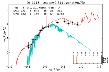
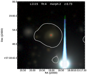
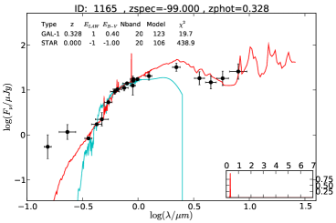
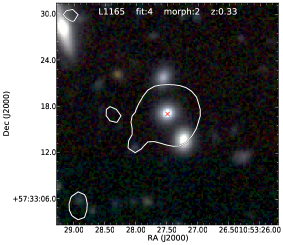
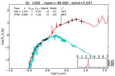
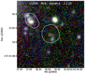
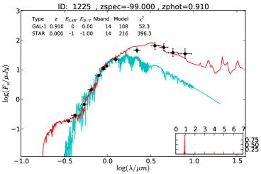
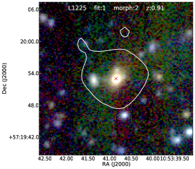
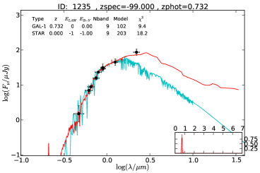
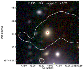
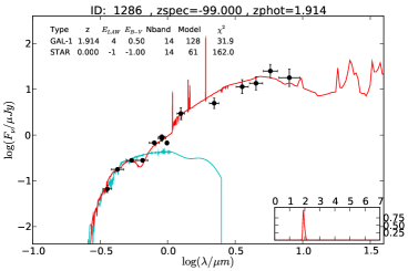
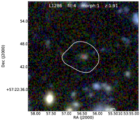
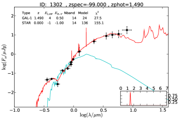
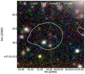
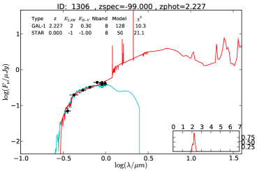
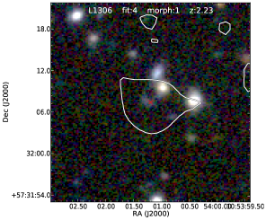
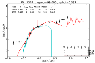
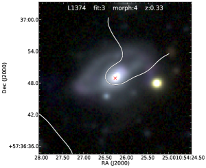
Figure 22: (Continued)

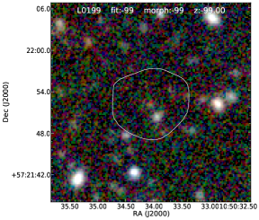
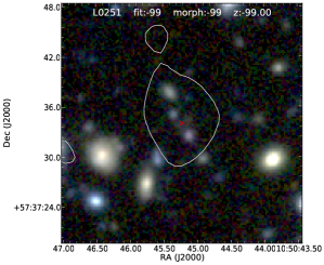
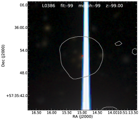
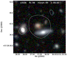
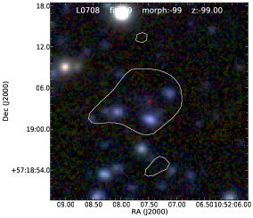
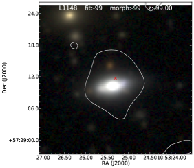
Figure 23: RGB images of sources with uncatalogued, blended, or otherwise unavailable counterparts, made using the same settings as used for Fig. 22. In L0199, L0251, L0386 and L0708 very faint, but uncatalogued counterparts can be seen in the images; in L0506 and L1148 the VLBA detection is offset from the foreground object by so much that an association was deemed unlikely.

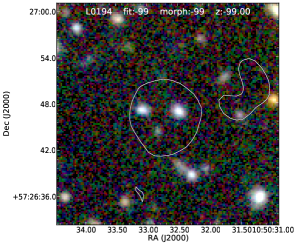
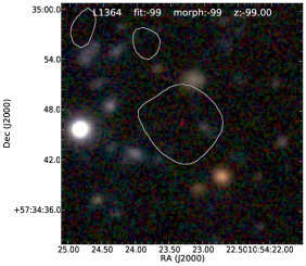
Figure 24: RGB images of sources with no visible counterparts, made using the same settings as used for Fig. 22.

We cross-matched the catalogues to our data by visual inspection, and by overplotting the locations of the radio, Spitzer/IRAC, and optical positions to ensure that the emission originated from the same object in each case. Because of the depth of the available data and the highly accurate astrometry of the VLBA observations we are confident that a simple match in coordinates provides the correct counterpart. It was found that the VLBA position and the optical position were in very good agreement. The mean separation between the two positions was 0.28 arcsec, with a maximum of 0.88 arcsec. In a first attempt, optical counterparts were searched using a 3 arcsec radius. All sources with separations of $>1$ arcsec between the radio and optical positions were found to be chance coincidences upon closer inspection of the images, and so a 1 arcsec search radius, followed by visual inspection, was adopted for cross-identification. Of our 65 VLBA-detected sources, 10 were located outside the region covered by the optical data, 47 had reliable optical counterparts (shown in Fig. 22), and 6 had either faint or uncatalogued counterparts, sometimes because of blending, or were overlapping with image artifacts such as diffraction spikes (L0199, L0251, L0386, L0506, L0708, L1148, see Fig. 23). The remaining 2 had no identifiable counterparts at all (L0194, L1364, see Fig. 24).

In two objects, L0506 and L1148 (Fig. 23), the position of the VLBA source is at the very edge of a clearly visible optical source, but a cross-identification with these objects was deemed unlikely. In L0506, a small extension to the optical source can be seen, indicating that two objects are blending and a reliable cross-identification can not be made. In L1148 both the VLA and the VLBA positions are offset from the foreground object by more than 1 arcsec. The nature of the three sources without any optical counterpart (Fig. 24) is puzzling. Radio sources with extremely faint or invisble optical or infrared counterparts have recently gained some attention (see, e.g., Higdon et al. 2005; Middelberg et al. 2011b; Norris et al. 2011a), and the speculation is that they are similar to high-redshift radio galaxies. But our data do not allow any further conclusions to be drawn.

Figure 19 presents the $R_{c}$ band distribution of the optical counterparts as a function of the radio flux density. We also plot the line of $\log(S_{1.4}/R_{c})=1.4$ which, according to Padovani (2011), defines the separation between star-forming galaxies and radio-quiet AGN in the top-left corner, and radio-loud AGN in the bottom-right corner. We find that the majority of the sources are classified as radio-loud (33/47), while 11 out of the 47 are located on the line. Only 3 objects are classified as star-forming galaxies or radio-quiet AGN.

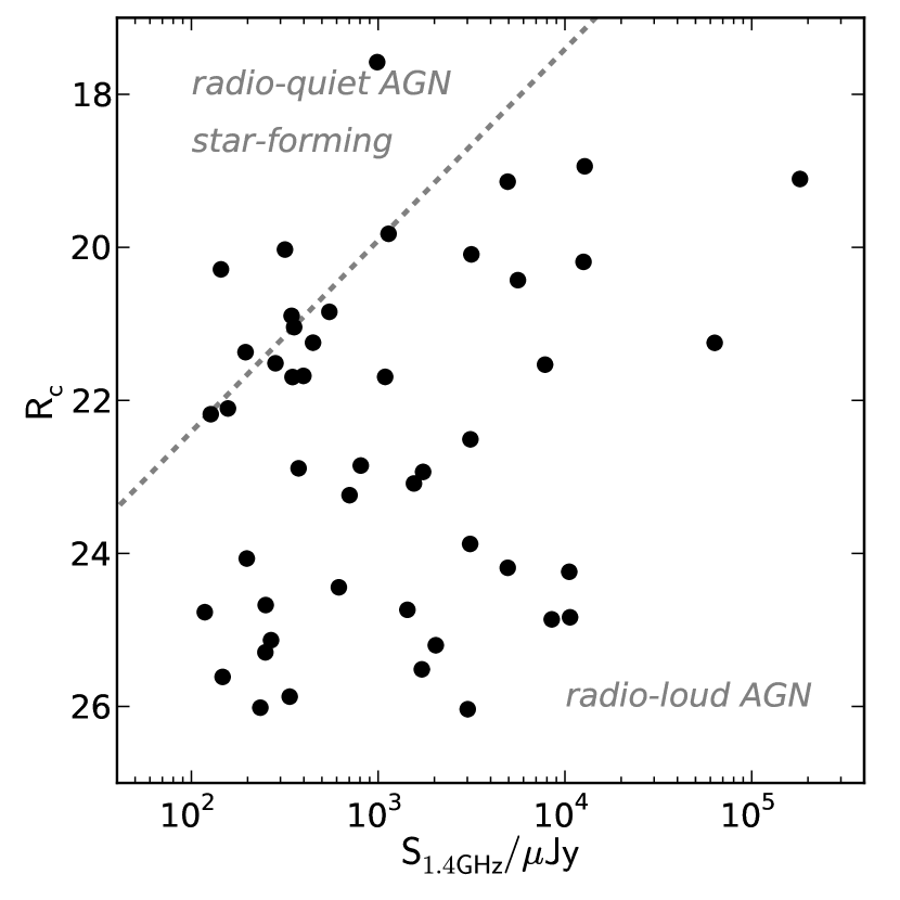
Figure 19: $R_{c}$ magnitude vs. VLA flux density for the 47 sources with optical counterparts (for source L0953 the SDSS $r$ magnitude was used). The majority of the population is classified as radio-loud. The limit for the radio loud population is given by the grey dashed line indicating $\rm{\log(S_{\rm VLA}/R_{c})=1.4}$.

In Fig. 20, we plot the X-ray flux versus VLA flux density for the sources located in the area observed by XMM-Newton. The lines in the plot show the loci occupied by X-ray AGN (dash-dotted line), radio-quiet AGN (dotted line), star-forming objects (dashed line) and radio galaxies (solid line), as presented in Padovani (2011). Out of the 47 sources with optical counterparts 26 are inside the area observed by XMM-Newton, and only 10 are detected in the X-rays ($F_{\rm lim,0.5-2\,keV}=1.9\times 10^{-16}\,{\rm erg/s/cm^{2}}$). The low number of X-ray dected sources does not allow one to draw statistically meaningful conclusions about the population. Roughly we can see that the X-ray sources are preferentially occupying the locus between star-forming and radio galaxies. We also include upper limits for the 16 sources inside the XMM-Netwon area which fall below the X-ray flux limit. These sources show similar behaviour to the dected sample, with the majority occupying the area between star-forming and radio galaxies.

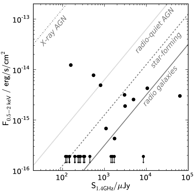
Figure 20: X-ray flux versus VLA flux density for the 26 sources inside the area covered by XMM-Newton. The lines denote the area occupied by X-ray AGN (dash-dotted line), radio-quiet AGN (dotted line), star-forming objects (dashed line) and radio galaxies (solid line), as presented in Padovani (2011). Upper limits are drawn for the 16 sources below the X-ray flux limit.

In order to classify properly the sources and rank the reliability of each SED fit, colour images for all 55 sources with optical coverage were produced. In Fig. 22 we show all of them togheter with the best SED fitting and photometric redshift computation. The following two subsections present the main result from this exercise.

5.6.1 Variety of radio source host galaxy morphologies

The host galaxies of the detected sources display a great variety in morphology. We have attempted to coarsely group them by visual appearance into 0 – point-like (as L0227), 1 – unresolved (as L0119), 2 – early type or bulge dominated (as L0449 and L0876, respectively), 3 – unclassified (as L0256) and 4 – spiral (as L1374, our only clear, though lopsided, spiral).

Sources in the “unresolved” or “unclassified” groups (coded 1 or 3, respectively) are just that – unresolved, or barely larger than the point spread function. However, they are mostly very faint, so one cannot tell if the faint speck that is seen in an image is only the brightest part of a much larger object. In an expanding universe, the surface brightness of an object decreases with $(1+z)^{4}$, a situation known as the “Tolman effect” (Tolman 1930). Therefore extended but faint parts of objects quickly become very difficult to detect as their redshift increases. Some objects in this category could also reasonably be assigned to the “ellipticals” subset (L0423, L0997), but judging by the visual appearance this is a matter of taste.

The “bulge dominated’ group (coded 2) mostly are circular, extended objects with a more or less pronounced surface brightness gradient towards the edges. Some have clearly extended halos as one typically finds in cD galaxies (L0449, L0846), while others have less pronounced halos (L0535).

In total 21 sources (45 %) were classified as unresolved/unclassified, 23 sources (49 %) as bulge-dominated, 2 (4 %) as point-like and 1 (2 %) as a spiral. To determine if this is correlated with the selection of VLBA-detected sources we have selected a control sample of 66 VLBA-undetected radio sources which were selected to have a similar distribution of VLA flux density as the VLBA-detected sources. Since most bright sources were detected, the control sample had a slight deficiency in bright sources and a slight overabundance of fainter sources. Out of the 66 sources in the control sample, only 36 had reliable counterparts, but these counterparts displayed a similar variety in host galaxy types. Since 22 out of the 25 morphologically classified objects are early-type objects, we can conclude that the VLBA radio sources are found in the expected hosts. This also agrees well with distribution of sources in the $R_{c}$ vs. VLA flux density diagram in Fig. 19, where the majority of the sources are in the radio-loud regime.

5.6.2 The SED models of radio source host galaxies

Using the photometric redshift estimation code LePhare, normal galaxy and AGN templates were fitted to the photometric points (see Ilbert et al. 2009; Salvato et al. 2009, 2011 for a detailed description of the fitting procedure). The normal galaxy templates include extinction values of E(B-V) = 0.00, 0.05, 0.10 - 0.50 (in steps of 0.1, see Fotopoulou et al. 2012 for details). Spiral and starburst templates (Sb-SB3) include extinction according to the Small Magellanic Cloud (SMC) law given in Prevot et al. (1984). This law is also used for the library of AGN and hybrids. Bluer templates (SB4-SB11) include extinction laws from Calzetti et al. (2000) and a modified Calzetti law (Ilbert et al. 2009), while templates redder than Sb (ellipticals and S0) include no further exctinction. In addition to the best photometric redshift solution LePhare also provides the full probability distribution function (PDFz), $F(z)=\exp{(\chi^{2}_{\rm min}(z)/2)}$. This distribution is calculated for a predefined redshift range ($0<z<7$ for this work) and is plotted as an inset in Fig. 22. In general, a source with a broad PDFz does not have a well-constrained redshift solution.

Clearly, the accuracy of the fit is depending on the number, wavelength and depth of bands available (depending on the redshift of the source a band is more or less crucial to identify specific spectral features). The fit also depends on whether the source varied in flux (typical AGN behaviour) within the time scale of the observations,and on contamination of photometry from objects within the aperture used to compute the flux (in this case 3 arcsec diameter). We could not identify quantifiable criteria, such as number of available bands, or reduced $\chi^{2}$ of the fit, to judge the quality of the models. Instead, we rated the fits according to the following guidelines:

• 1: a bad fit due to a limited number of bands (less than 6) or because the source is at the border of the imaged field (see for example L0140).

• 2: a doubtful fit because the photometry is effected by blending with nearby objects (see for example L0352).

• 3: a potential AGN (doubtful fit): the lack of Xray information did not allow the use of proper template (see example L0227).

• 4: the optical photometry is not contaminated and the number of bands is sufficient.

We do not discuss here sources with a SED fit rated 1 and 2 for obvious reasons. Only two sources are rated 3 (L0227 and L1374), classified as potential AGN due to their morphological appearance and due to the typical power-law seen in the mid-infrared bands. These objects lie outside the XMM area and thus were treated as normal galaxies during the photometric redshift estimation. Following the definition of SEDs as in Fotopoulou et al. (2012) and Salvato et al. (2011) we classified the 30 sources with a good fit as following: 11 present a typical SED of a early type galaxy, 6 are best modelled as spirals, and 12 are classified as starburst (either pure starburst or X-ray detected but still starburst dominated). Three of the 12 objects classified as starburst are clearly early-type objects by visual appearance. The erroneous SED fit is a clear and well-known case of degeneracy where a starburst template with heavy extinction (0.3, 0.35 and 0.4 of E(B-V), as visible in the plot of L0397 and L0911 and L1165) can mimic an early-type template (see also the discussion in Onodera et al. 2012). In the case of L0973 the image clearly indicates an early-type the best fit is obtained with the template of M82. Unlike the other starburst templates that are theoretical, this one is empirical and already includes dust. For this reason we group this source with the 3 described above. For the remaining 8 sources fit by a starburst template the applied extinction is very high but we can not prove that this are early type because they are morphologically unresolved.

6 Conclusions

The main results from this work are summarised as follows:

• VLBI observations of 217 sources have been carried out with the VLBA. Primary beam corrections have been developed and tested using dedicated observations, and a novel multi-source self-calibration scheme has improved the coherence of the data significantly. Data from overlapping pointings were added to improve the sensitivity in the overlap regions (mosaicing). Images were made of all targets, and 65 sources were detected, a fraction of 30 %. Data from the literature were added for interpretation. VLBI observations with hundreds of pointings are now feasible and can be added to large surveys carried out at other wavelengths.

• The VLBA-detected sources have larger spectral indices than the non-detected sources, which is consistent with their emission coming from more compact regions near the AGN. Above a spectral index of $\alpha=0.0$, almost all sources (14/17) are detected, confirming that spectral index is a strong selection criterion for radio AGN. Using the difference between the flux densities measured with the VLA and the VLBA as a measure for star forming activity, a positive correlation has been found between the star formation and AGN activity. This correlation indicates that interactions between the radio ejecta and the host galaxy tend to increase, and not disrupt, star formation.

• Source counts of VLBA-detected, faint radio sources are presented for the first time. They form a lower limit on the fraction of radio AGN among the radio source population. At the bright end of the distribution the counts line up with literature values, indicating that the majority of mJy sources is AGN-powered. At the sub-mJy level, the counts drop below the sub-mJy plateau seen at arcsec-scale resolution but seem to exhibit a similar flattening. A significant fraction of the sub-mJy, 15 % to 25 %, are AGN-driven. However, the high resolution of the VLBA observations implies that some AGN-driven radio sources are not detected, and so it is expected that the correct fraction of AGN-driven sources is higher.

• Using literature data we discuss the multiwave-length properties of the counterparts to 47 of the 65 VLBA-detected radio sources. For about 50 % of the sources the morphology suggests the host to be an early-type galaxy. For the rest of the sources the image quality and the redshift do not allow to make any assessment of the morphology. In many cases the best fit is obtained with the template of a heavily extinct startburst. This is a well-known case of degeneracy in SED fitting where these kinds of templates plus extinction mimic an early-type object. Globally, the typical hosts of VLBI sources are passive galaxies, in agreement with previous results.

With software correlators, accurate primary beam corrections and multi-source self-calibration, wide-field VLBA observations have become practical and versatile. The calibration strategies will certainly improve, and larger bandwidths of future instruments will make such observations easier because the instantaneous sensitivity increases.

The significance of wide-field VLBI observations has been acknowledged by NRAO during the last call for proposals, in accepting a 276 h proposal for a sensitive survey of the 2 deg² field of the COSMOS survey with the VLBA, to observe almost 3000 sub-mJy radio sources. This survey will greatly simplify the data analysis since it will result in a uniform sensitivity over a large region. Furthermore, a 200 h project has been accepted, aiming at carrying out snapshot observations of more than 10 000 FIRST sources over 100 deg². The data from these two projects taken together, and adding statistics from all-sky surveys of VLBI calibrator sources, will allow a construction of the source counts of VLBI-detected sources from the Jy to the $\mu$Jy regime.

7 Appendix A

Table 6: Data of the 217 sources which were in principle detectable ($S_{\rm VLA}>6\times{\rm rms}$). Col 1: source ID used in this paper; Col 2: source designation used by Ibar et al. (2009); Cols 3,4: 610 MHz and 1.4 GHz flux densities; Cols 5: spectral index calculated from cols. 3,4; Col 6: rms of the VLBA observations (uniform weighting); Col 7-10: peak and integrated flux densities of the VLBI observations and their associated errors (uniform weighting); Col 11,12: flux-weighted position of the VLBI source (uniform weighting)

ID	Name	$S_{610}$	$S_{\rm VLA}$	$\alpha$	rms	$S_{\rm p}$	$\Delta S_{\rm p}$	$S_{\rm VLBA}$	$\Delta S_{\rm VLBA}$	RA	Dec
		$\mu$Jy	$\mu$Jy		$\mu$Jy/beam	$\mu$Jy/beam	$\mu$Jy/beam	$\mu$Jy	$\mu$Jy	deg	deg
(1)	(2)	(3)	(4)	(5)	(6)	(7)	(8)	(9)	(10)	(11)	(12)
L0003	LH1.4GHzJ104849.8+571415	19386	10840	-0.70
L0009	LH1.4GHzJ104858.3+570925	1709	1384	-0.25	102	462	112	642	121	162.242958361	57.157160902
L0012	LH1.4GHzJ104905.1+571151	26691	14612	-0.73
L0016	LH1.4GHzJ104914.8+570508	1029	529	-0.80
L0025	LH1.4GHzJ104922.9+571901	4994	2425	-0.87	76	939	121	2209	234	162.345288947	57.317164956
L0034	LH1.4GHzJ104934.3+570608		14787		74	323	81	295	80	162.393862805	57.103353297
L0049	LH1.4GHzJ104943.8+571737	1008	1013	0.01	52	541	75	666	84	162.432542797	57.29366112
L0051	LH1.4GHzJ104944.1+570628	1823	1275	-0.43	66	528	85	916	113	162.433765316	57.108035949
L0055	LH1.4GHzJ104947.8+571354	689	607	-0.15	54	423	69	490	73	162.4489331	57.231806689
L0061	LH1.4GHzJ104950.4+570120c		5266
L0066	LH1.4GHzJ104951.3+572812	967	1083	0.14	75	713	104	922	119	162.463891893	57.470082634
L0077	LH1.4GHzJ104954.2+570456	1363	1376	0.01	66	541	86	633	91	162.475858493	57.082238326
L0081	LH1.4GHzJ104956.7+570647	596	335	-0.69
L0082	LH1.4GHzJ104956.8+571042	2053	1046	-0.81
L0087	LH1.4GHzJ104958.0+570727	1082	650	-0.61
L0100	LH1.4GHzJ105002.0+571622	213	232	0.10
L0117	LH1.4GHzJ105007.3+571652	452	257	-0.68
L0119	LH1.4GHzJ105008.1+572018	3486	2035	-0.65	43	647	78	1195	127	162.533539506	57.338390632
L0130	LH1.4GHzJ105010.4+570724b	1876	5598	1.32	54	1291	141	2335	240	162.538743032	57.121401186
L0140	LH1.4GHzJ105012.6+571137	1280	616	-0.88	42	235	48	415	59	162.552329219	57.193600719
L0144	LH1.4GHzJ105014.4+572844	689	416	-0.61
L0149	LH1.4GHzJ105015.6+570258	5060	3155	-0.57	64	687	94	983	117	162.564968684	57.048810568
L0160	LH1.4GHzJ105019.7+572812	662	266	-1.10
L0165	LH1.4GHzJ105023.4+572439	485	253	-0.78
L0171	LH1.4GHzJ105025.5+570453	266	250	-0.07	55	275	62	271	61	162.606338811	57.081508924
L0173	LH1.4GHzJ105026.3+570744	1270	793	-0.57
L0181	LH1.4GHzJ105029.2+571427	2450	1286	-0.78
L0183	LH1.4GHzJ105029.6+571036	417	203	-0.87
L0189	LH1.4GHzJ105032.0+572027	5184	723	-2.37
L0194	LH1.4GHzJ105032.7+572646	371	466	0.27	41	364	55	497	64	162.636123187	57.446286836
L0197	LH1.4GHzJ105033.1+571703	388	169	-1.00
L0199	LH1.4GHzJ105034.0+572152	1830	1005	-0.72	36	214	42	220	42	162.641811126	57.364553024
L0201	LH1.4GHzJ105034.2+572922	712	336	-0.90
L0211	LH1.4GHzJ105035.9+572318	4128	1768	-1.02
L0217	LH1.4GHzJ105037.6+572844	701	420	-0.62
L0225	LH1.4GHzJ105039.1+565806	2554	1520	-0.62
L0227	LH1.4GHzJ105039.6+572336	4326	4936	0.16	36	2687	272	3972	399	162.664768172	57.393502619
L0231	LH1.4GHzJ105040.7+573308	959	703	-0.37	54	740	92	984	112	162.669491607	57.552292637
L0234	LH1.4GHzJ105042.0+570706	1516	770	-0.82
L0251	LH1.4GHzJ105045.2+573734	1286	858	-0.49	76	348	84	290	81	162.688439094	57.626114051
L0256	LH1.4GHzJ105045.9+570822	430	344	-0.27	39	164	42	153	42	162.691253621	57.139547122
L0263	LH1.4GHzJ105048.2+571614	336	165	-0.86
L0273	LH1.4GHzJ105050.5+570715	856	386	-0.96
L0284	LH1.4GHzJ105053.4+572426	568	279	-0.86
L0290	LH1.4GHzJ105054.6+570810	841	344	-1.08
L0301	LH1.4GHzJ105056.6+571532	1542	700	-0.95
L0302	LH1.4GHzJ105056.6+571631	557	324	-0.65
L0320	LH1.4GHzJ105100.9+572036	751	322	-1.02
L0328	LH1.4GHzJ105101.9+573445	3371	1332	-1.12
L0339	LH1.4GHzJ105104.9+572719	348	153	-0.99
L0342	LH1.4GHzJ105104.7+570150b		4050
L0346	LH1.4GHzJ105105.8+571057	699	421	-0.61
L0352	LH1.4GHzJ105106.7+571152	255	355	0.40	32	163	36	282	43	162.777939135	57.197994694
L0354	LH1.4GHzJ105107.7+570205		314
L0380	LH1.4GHzJ105113.2+574156	2490	1152	-0.93
L0381	LH1.4GHzJ105113.4+571426	1455	763	-0.78
L0382	LH1.4GHzJ105113.5+572654	440	283	-0.53
L0386	LH1.4GHzJ105115.0+573552	4841	2362	-0.86	47	168	50	133	49	162.812383572	57.597906246
L0397	LH1.4GHzJ105117.6+571639	552	398	-0.39	27	265	38	411	49	162.823463843	57.277592149
L0399	LH1.4GHzJ105118.0+571920	218	131	-0.61
L0408	LH1.4GHzJ105120.0+570954	1209	601	-0.84
L0409	LH1.4GHzJ105120.4+572253	399	238	-0.62
L0411	LH1.4GHzJ105120.8+573037	439	336	-0.32	32	205	38	294	44	162.83673954	57.510376172
L0412	LH1.4GHzJ105120.9+573532	9061	8496	-0.08	45	4679	472	8966	898	162.836886524	57.592367389
L0416	LH1.4GHzJ105121.5+573613		563
L0420	LH1.4GHzJ105122.1+570854	18706	10644	-0.68	36	2080	212	10562	921	162.841971832	57.148560655
L0423	LH1.4GHzJ105122.9+573228	1928	1434	-0.36	34	642	73	1343	138	162.845349839	57.541242785
L0427	LH1.4GHzJ105123.6+570849	697	459	-0.50
L0437	LH1.4GHzJ105125.7+573544	945	577	-0.59
L0447	LH1.4GHzJ105127.5+573620		362
L0449	LH1.4GHzJ105127.8+570854		12570		36	337	49	506	62	162.86695653	57.150285403
L0452	LH1.4GHzJ105128.1+573502	585	361	-0.58
L0465	LH1.4GHzJ105130.5+573808	444	259	-0.65
L0468	LH1.4GHzJ105130.5+574407		924
L0477	LH1.4GHzJ105132.4+571114	22200	12756	-0.67	32	823	89	1157	120	162.884787347	57.18764161
L0484	LH1.4GHzJ105134.1+570922	177	348	0.81	34	261	43	278	44	162.892178451	57.156140392
L0492	LH1.4GHzJ105135.5+572739	324	182	-0.69
L0498	LH1.4GHzJ105136.1+572959	605	302	-0.84
L0500	LH1.4GHzJ105136.2+573302	955	537	-0.69

Table 6: (Continued)

ID	Name	$S_{610}$	$S_{\rm VLA}$	$\alpha$	rms	$S_{\rm p}$	$\Delta S_{\rm p}$	$S_{\rm VLBA}$	$\Delta S_{\rm VLBA}$	RA	Dec
		$\mu$Jy	$\mu$Jy		$\mu$Jy/beam	$\mu$Jy/beam	$\mu$Jy/beam	$\mu$Jy	$\mu$Jy	deg	deg
(1)	(2)	(3)	(4)	(5)	(6)	(7)	(8)	(9)	(10)	(11)	(12)
L0502	LH1.4GHzJ105136.4+570129	1623	803	-0.85
L0505	LH1.4GHzJ105136.9+573751	1129	514	-0.95
L0506	LH1.4GHzJ105137.0+572940	4179	2532	-0.60	28	295	41	402	49	162.904118977	57.494500938
L0507	LH1.4GHzJ105137.7+574454	2746	1036	-1.17
L0513	LH1.4GHzJ105139.1+573043		441
L0529	LH1.4GHzJ105141.4+571951	626	372	-0.63
L0534	LH1.4GHzJ105142.0+571501	392	201	-0.80
L0535	LH1.4GHzJ105142.0+573447	483	1090	0.98	35	885	96	1168	122	162.925189291	57.579945389
L0536	LH1.4GHzJ105142.1+573554		4940		38	982	106	1243	130	162.925392256	57.59848336
L0548	LH1.4GHzJ105143.7+572937	891	432	-0.87
L0553	LH1.4GHzJ105144.5+570555		300
L0555	LH1.4GHzJ105144.5+571719	294	150	-0.81
L0578	LH1.4GHzJ105148.7+573248	835	807	-0.04	30	747	81	944	99	162.952962275	57.546820439
L0593	LH1.4GHzJ105150.1+572635	177	118	-0.49	24	246	34	272	36	162.958786403	57.443275605
L0595	LH1.4GHzJ105150.3+573244	35615	16418	-0.93
L0603	LH1.4GHzJ105151.7+572636	238	127	-0.76
L0604	LH1.4GHzJ105152.0+570907	305	208	-0.46
L0607	LH1.4GHzJ105152.4+570950	4951	3118	-0.56	34	1005	107	2965	216	162.968238773	57.163967637
L0644	LH1.4GHzJ105158.3+570913	372	214	-0.67
L0648	LH1.4GHzJ105158.9+572330	121	234	0.79	23	177	29	304	38	162.9954889	57.391705693
L0653	LH1.4GHzJ105159.4+570013b		2059
L0665	LH1.4GHzJ105201.1+565947	2181	480	-1.82
L0667	LH1.4GHzJ105201.3+572445	104	120	0.17
L0669	LH1.4GHzJ105201.9+574051	611	260	-1.03
L0679	LH1.4GHzJ105204.2+572655	195	121	-0.57
L0687	LH1.4GHzJ105205.0+572917	250	130	-0.79
L0691	LH1.4GHzJ105205.5+571710	115	141	0.25
L0698	LH1.4GHzJ105206.1+565704		2136
L0703	LH1.4GHzJ105206.5+574109	13423	10542	-0.29	50	2828	289	8420	555	163.026882769	57.686063698
L0705	LH1.4GHzJ105207.2+570745	560	287	-0.80
L0708	LH1.4GHzJ105207.5+571903		324		24	275	37	269	36	163.031206078	57.31778852
L0722	LH1.4GHzJ105210.6+571203	289	172	-0.62
L0724	LH1.4GHzJ105211.0+572908	2917	1713	-0.64	24	1064	110	1585	160	163.045937557	57.485563316
L0736	LH1.4GHzJ105212.5+572453	466	278	-0.62
L0739	LH1.4GHzJ105213.4+571605	574	301	-0.78
L0750	LH1.4GHzJ105215.0+572635	299	161	-0.75
L0760	LH1.4GHzJ105216.6+573530	296	194	-0.51
L0763	LH1.4GHzJ105216.9+572017	215	126	-0.64
L0767	LH1.4GHzJ105217.6+572127	445	216	-0.87
L0776	LH1.4GHzJ105219.1+571857	219	123	-0.69
L0800	LH1.4GHzJ105224.5+570838	3944	2639	-0.48
L0805	LH1.4GHzJ105225.3+571131	275	174	-0.55
L0809	LH1.4GHzJ105225.6+573322	8663	4873	-0.69
L0810	LH1.4GHzJ105225.8+570152	975	696	-0.41
L0824	LH1.4GHzJ105227.4+571415	268	154	-0.67
L0838	LH1.4GHzJ105229.1+571242	236	189	-0.27
L0845	LH1.4GHzJ105230.5+570853	551	314	-0.68
L0846	LH1.4GHzJ105230.6+571312	373	282	-0.34	30	198	36	291	42	163.12756064	57.220099911
L0851	LH1.4GHzJ105231.1+573501	278	233	-0.21
L0860	LH1.4GHzJ105231.8+570650	539	1137	0.90	49	582	76	1015	113	163.132553769	57.114020856
L0862	LH1.4GHzJ105232.3+572447	293	234	-0.27
L0867	LH1.4GHzJ105232.4+570842	565	212	-1.18
L0870	LH1.4GHzJ105232.9+572542	320	148	-0.93
L0876	LH1.4GHzJ105234.0+573057		144		25	113	28	143	29	163.141622298	57.515886497
L0879	LH1.4GHzJ105234.9+572641	255	134	-0.77
L0882	LH1.4GHzJ105235.4+572652	484	236	-0.86
L0890	LH1.4GHzJ105237.3+573103		63323		25	551	61	607	66	163.15566438	57.517692521
L0891	LH1.4GHzJ105237.4+572148	280	175	-0.57
L0902	LH1.4GHzJ105239.6+572431	257	142	-0.71
L0903	LH1.4GHzJ105239.7+573054	227	139	-0.59
L0911	LH1.4GHzJ105241.4+572320	2435	1740	-0.40	23	160	28	184	30	163.172665445	57.389069831
L0917	LH1.4GHzJ105242.4+572444	342	267	-0.30
L0918	LH1.4GHzJ105242.4+571914	602	349	-0.66
L0927	LH1.4GHzJ105243.3+574813	1013	1857	0.73	100	1313	166	1237	159	163.180471707	57.803888368
L0933	LH1.4GHzJ105245.3+573616	619	448	-0.39	31	261	41	267	41	163.188933432	57.604521945
L0953	LH1.4GHzJ105250.0+574450	1682	988	-0.64	65	334	73	309	72	163.208413838	57.747505888
L0966	LH1.4GHzJ105252.8+570753	553	292	-0.77
L0968	LH1.4GHzJ105252.8+572859	538	212	-1.12
L0973	LH1.4GHzJ105254.2+572341	170	157	-0.10	24	143	28	140	28	163.226115327	57.39499839
L0975	LH1.4GHzJ105255.1+571944		140
L0977	LH1.4GHzJ105255.3+571950	4514	3107	-0.45	26	1480	151	2921	293	163.23051676	57.330690586
L0987	LH1.4GHzJ105256.8+570825	910	522	-0.67
L0997	LH1.4GHzJ105258.0+570834	529	375	-0.41	52	284	59	471	70	163.241765558	57.14302443
L1007	LH1.4GHzJ105259.3+573226	298	232	-0.30
L1020	LH1.4GHzJ105301.3+570543	1697	945	-0.70
L1022	LH1.4GHzJ105301.7+572520	361	257	-0.41
L1025	LH1.4GHzJ105302.6+571813	209	143	-0.46
L1028	LH1.4GHzJ105303.4+573527		210
L1029	LH1.4GHzJ105303.7+571205	627	417	-0.49
L1031	LH1.4GHzJ105303.9+573532		323

Table 6: (Continued)

ID	Name	$S_{610}$	$S_{\rm VLA}$	$\alpha$	rms	$S_{\rm p}$	$\Delta S_{\rm p}$	$S_{\rm VLBA}$	$\Delta S_{\rm VLBA}$	RA	Dec
		$\mu$Jy	$\mu$Jy		$\mu$Jy/beam	$\mu$Jy/beam	$\mu$Jy/beam	$\mu$Jy	$\mu$Jy	deg	deg
(1)	(2)	(3)	(4)	(5)	(6)	(7)	(8)	(9)	(10)	(11)	(12)
L1034	LH1.4GHzJ105304.5+571547	143	198	0.39	30	183	35	155	34	163.268708013	57.263232348
L1036	LH1.4GHzJ105304.8+573055	755	501	-0.49
L1040	LH1.4GHzJ105305.3+572330	192	147	-0.32
L1052	LH1.4GHzJ105308.1+572222	355	317	-0.14	25	127	28	145	29	163.283666617	57.37303887
L1059	LH1.4GHzJ105309.3+571659		462
L1061	LH1.4GHzJ105309.5+573712	416	294	-0.42
L1062	LH1.4GHzJ105309.5+570636	887	585	-0.50
L1067	LH1.4GHzJ105310.6+573435	316	190	-0.61
L1077	LH1.4GHzJ105312.2+571105	947	420	-0.98
L1080	LH1.4GHzJ105312.7+573111	822	429	-0.78
L1092	LH1.4GHzJ105314.0+572448		127		25	174	30	142	29	163.308246293	57.413486699
L1094	LH1.4GHzJ105314.2+573020	725	345	-0.89
L1106	LH1.4GHzJ105316.8+573550	492	294	-0.62
L1108	LH1.4GHzJ105317.4+572722	185	132	-0.41
L1112	LH1.4GHzJ105318.8+574546		531
L1113	LH1.4GHzJ105318.9+572140	767	447	-0.65
L1115	LH1.4GHzJ105319.0+571851	908	548	-0.61	29	144	32	229	37	163.329236431	57.314387781
L1132	LH1.4GHzJ105322.4+573652	322	192	-0.62
L1136	LH1.4GHzJ105322.8+571500	597	509	-0.19
L1139	LH1.4GHzJ105323.5+571733	305	185	-0.60
L1144	LH1.4GHzJ105324.6+571658	975	567	-0.65
L1148	LH1.4GHzJ105325.3+572911	1031	602	-0.65	26	122	29	199	33	163.355459276	57.486609371
L1155	LH1.4GHzJ105326.7+571405	527	325	-0.58
L1165	LH1.4GHzJ105327.5+573316		195		29	260	39	219	36	163.364535455	57.554736564
L1166	LH1.4GHzJ105327.6+574543	12354	6618	-0.75
L1168	LH1.4GHzJ105328.0+571115	685	393	-0.67
L1197	LH1.4GHzJ105335.2+572921	578	373	-0.53
L1200	LH1.4GHzJ105335.8+572157	88	147	0.62	30	194	36	226	38	163.399383286	57.365923937
L1204	LH1.4GHzJ105337.1+574315		354
L1206	LH1.4GHzJ105337.3+574240	1432	1157	-0.26
L1210	LH1.4GHzJ105338.2+574211	702	365	-0.79
L1225	LH1.4GHzJ105340.9+571952	2332	1554	-0.49	34	262	43	283	44	163.420225248	57.331410611
L1227	LH1.4GHzJ105341.2+571920	262	163	-0.57
L1234	LH1.4GHzJ105342.1+573026	765	346	-0.96
L1235	LH1.4GHzJ105342.1+574436	12655	7825	-0.58	72	755	105	2152	194	163.425629443	57.743542688
L1239	LH1.4GHzJ105343.2+571633	366	285	-0.30
L1240	LH1.4GHzJ105343.3+572530		257
L1254	LH1.4GHzJ105346.9+571609	260	201	-0.31
L1266	LH1.4GHzJ105348.8+573034	303	205	-0.47
L1280	LH1.4GHzJ105354.1+574244	718	429	-0.62
L1286	LH1.4GHzJ105356.5+572244	462	249	-0.74	35	145	38	258	44	163.485255414	57.379118349
L1299	LH1.4GHzJ105359.9+572600	397	215	-0.74
L1302	LH1.4GHzJ105400.5+573321	4646	3016	-0.52	37	255	45	222	43	163.501801452	57.556002324
L1306	LH1.4GHzJ105401.2+573207	410	267	-0.52	36	143	39	142	39	163.505027094	57.535413357
L1325	LH1.4GHzJ105406.1+572413	311	190	-0.59
L1328	LH1.4GHzJ105406.8+571256	3558	1686	-0.90
L1344	LH1.4GHzJ105415.2+573336	359	220	-0.59
L1361	LH1.4GHzJ105421.2+572544	1725	1041	-0.61
L1364	LH1.4GHzJ105423.3+573446	1109	661	-0.62	50	415	65	598	78	163.597162837	57.579559074
L1371	LH1.4GHzJ105425.7+571937	695	376	-0.74
L1374	LH1.4GHzJ105427.0+573644	322140	181160	-0.69	58	1096	124	1658	176	163.609453312	57.613618513
L1402	LH1.4GHzJ105440.6+571647	2859	1976	-0.44
L1404	LH1.4GHzJ105442.1+571639	3366	2778	-0.23	98	769	125	945	136	163.675525388	57.277615166
L1409	LH1.4GHzJ105445.9+572747	999	389	-1.14
L1423	LH1.4GHzJ105456.3+573017	662	514	-0.30
L1424	LH1.4GHzJ105458.5+572035	1104	884	-0.27
L1425	LH1.4GHzJ105458.6+572828	689	570	-0.23
L1436	LH1.4GHzJ105516.0+573257		7104

Table 7: Multi-wavelength data for the VLBI-detected sources. Column 1: source ID used in this paper; Column 2: ID from Fotopoulou et al. (2012), $-99$: outside imaged area, -1: uncatalogued/blended counterpart, 0: no visible counterpart; Column 3: $R_{c}$ AB magnitude; Column 4: $3.6\,\mu$m AB magnitude from the SWIRE survey; Column 5: spectroscopic redshift, where available; Column 6: best photometric redshift; Column 7: morphology flag, 0: point-like, 1 – unresolved, 2 – early type or bulge-dominated, 3 – unclassified, 4 – spiral; Column 8: quality of the fit, 1: too few bands, 2: blended photometry, 3: doubful because of a lack of X-ray information, 4: a good fit; Column 9: model type used in the best fit for photometric redshift; Column 10: X-ray flux in the 0.5–2 keV band; Column 11: X-ray luminosity in the 0.5–2 keV band, $-99$: outside imaged area, 0: imaged, but undetected; Column 12: a “$<$” indicates that the X-ray luminosity is an upper limit; Column 13: hardness ratio calculated between the 0.5–2 keV and 2.0–4.5 keV bands.

ID	opt. ID	$R_{c}$	3.6 $\mu$m	${\rm z_{spec}}$	${\rm z_{phot}}$	morph.	fit	model	$F_{X}$(0.5–2 keV)	flag	$\log{L_{\rm X}}$(0.5–2 keV)	HR1
		mag	mag						$10^{-16}\,{\rm erg/s/cm^{2}}$		erg/s
(1)	(2)	(3)	(4)	(5)	(6)	(7)	(8)	(9)	(10)	(11)	(12)	(13)
L0009	-99
L0025	-99
L0034	-99
L0049	-99
L0051	-99
L0055	-99
L0066	-99
L0077	-99
L0119	166492	25.20			1.70	2	1	110	-99
L0130	42435	20.43		0.4239	0.34	2	1	131	-99
L0140	55191	24.44			4.20	1	1	126	-99
L0149	28661	20.09		3.2687	0.29	2	1	131	-99
L0171	34378	24.67			0.97	1	1	123	-99
L0194	0
L0199	-1
L0227	89171	19.14	18.69	1.439	0.27	0	3	129	-99
L0231	117241	23.24			0.87	2	1	108	-99
L0251	-1
L0256	45485	20.90		0.5396	0.60	3	1	101	-99
L0352	55842	21.04		0.593	0.91	2	2	129	-99
L0386	-1
L0397	69623	21.68	18.95		0.69	2	4	120	-99
L0411	187543	25.87	21.54		1.82	1	4	123	0	$<$	42.95
L0412	124257	24.86	21.39		2.12	1	4	122	0	$<$	43.14
L0420	46934	24.83			1.13	1	1	131	-99
L0423	114988	24.74	19.72		1.34	2	4	107	0	$<$	42.57
L0449	47368	20.19			0.55	2	1	109	-99
L0477	53986	18.94	17.83	0.3177	0.40	2	4	107	-99
L0484	48731	21.69			0.59	3	1	114	-99
L0506	-1
L0535	206628	21.69	18.89		0.58	2	4	2	6.8		42.11	-0.69
L0536	206644	24.19	20.47		1.73	1	2	114	25.5		44.02	-0.5
L0578	206598	22.85	18.99	0.99	1.00	1	4	5	48.9		43.61	0.03
L0593	97588	24.77	19.55		1.04	3	4	113	0	$<$	42.25
L0607	49780	22.51	19.27		1.16	3	4	119	-99
L0648	88715	26.02			2.07	1	4	130	0	$<$	43.12
L0703	206690	24.24	20.18	0.462	1.53	1	4	114	42.6		42.65	-0.62
L0708	-1
L0724	167757	25.51	20.13		1.51	3	4	113	0	$<$	42.72
L0846	59617	21.51	19.14		0.58	2	4	108	-99
L0860	40969	19.82		0.3826	0.52	2	1	102	-99
L0876	110535	20.29	19.12		0.54	2	4	102	0	$<$	41.47
L0890	206578	21.25	18.33	0.71	0.58	2	4	2	30.0		42.99	-0.53
L0911	206453	22.93	19.29	1.013	1.11	2	2	1	4.3		42.58	-0.63
L0927	-99
L0933	126512	21.25		0.493	0.53	2	4	113	0	$<$	41.37
L0953	170521		16.40	0.0731	0.29	2	4	101	-99
L0973	206457	22.11	19.74	0.762	0.68	0	4	5	122.7		43.69	-0.59
L0977	206416	23.88	18.59	1.45	1.30	1	4	18	18.9		43.67	-0.35
L0997	45980	22.89			0.96	1	4	102	-99
L1034	66996	24.07	19.72		1.33	1	4	115	0	$<$	42.56
L1052	85797	20.03	18.85		0.41	2	4	107	0	$<$	41.17
L1092	92439	22.18	19.09		0.62	2	4	108	0	$<$	41.63
L1115	206406	20.84	18.41	0.711	0.73	2	4	124	77.1		43.40	-0.65
L1148	-1
L1165	117627	21.37	20.75		0.33	2	4	123	0	$<$	40.91
L1200	84577	25.61	21.32		2.55	1	4	121	0	$<$	43.38
L1225	78963	23.09	19.37		0.91	2	1	108	0	$<$	42.09
L1235	151191	21.53			0.73	2	4	102	-99
L1286	175609	25.29	21.27		1.91	1	4	128	0	$<$	43.02
L1302	206717	26.04	21.54		1.49	1	4	124	31.5		43.92	-0.28
L1306	114090	25.13			2.23	1	4	128	0	$<$	43.21
L1364	0
L1374	128598	19.11	17.55		0.33	4	3	123	-99
L1404	-99

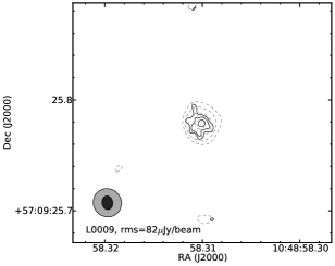
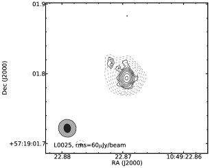
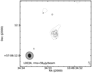
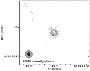
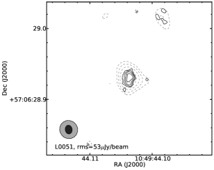
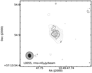
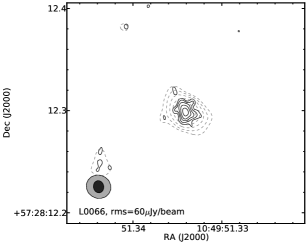
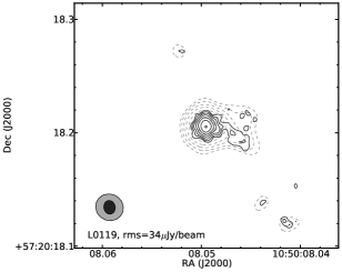
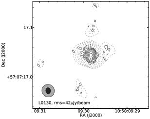
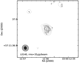
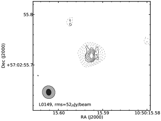
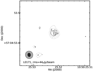
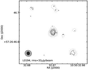
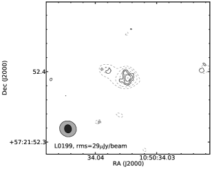
Figure 21: Contour plots of the VLBA images of the 65 detected sources. The plots show regions of 216 mas$\times$216 mas, centred on the sources, except for the plot of L0703, which shows a region of 360 mas$\times$360 mas. Black contours indicate the full-resolution, naturally-weighted images, whereas grey, dashed contours indicate images made with a 10 M$\lambda$ taper. The black and grey ellipses in the lower left corners indicate the size and orientation of the restoring beams used with full resolution and a 10 M$\lambda$ taper, respectively. In both cases contours start at the 3 times the naturally-weighted image noise and increase by factors of $\sqrt{2}$. The noise levels of the naturally weighted images have been added to the plots. Note that the flux densities listed in Tab. 6 have been extracted from uniformly-weighted images (not shown), to reduce the effect of the point spread function (see Sect. 4 and Fig. 10).

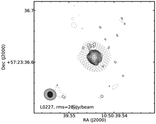
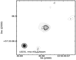
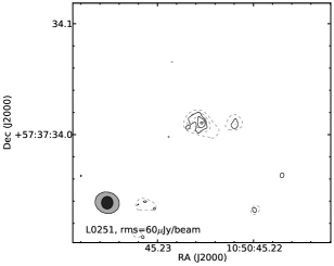
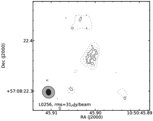
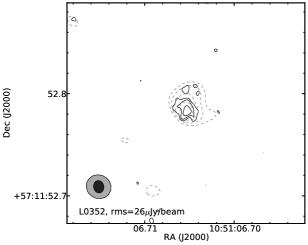
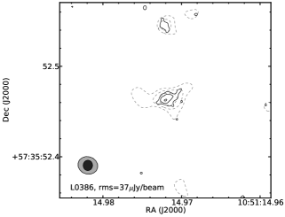
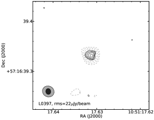
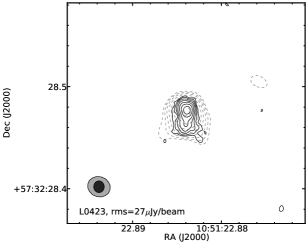
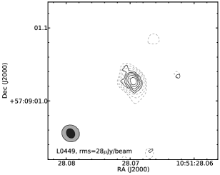
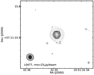
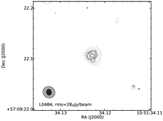
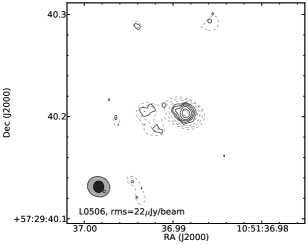
Figure 21: (Continued)

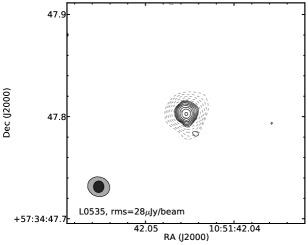
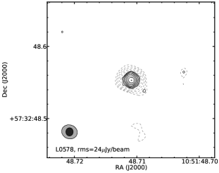
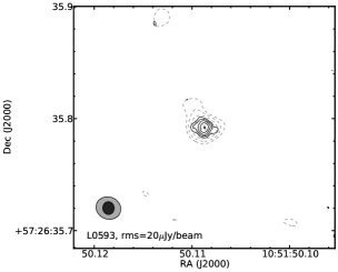
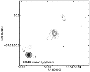
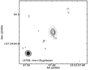
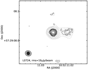
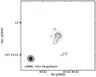
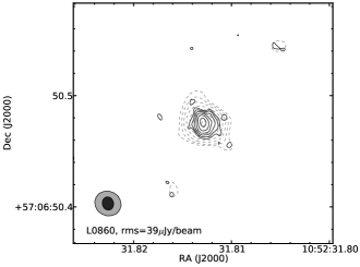
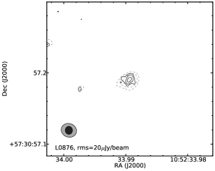
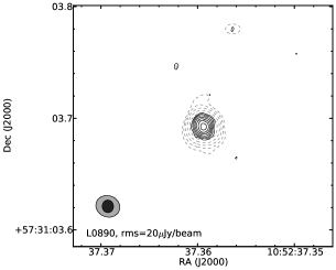
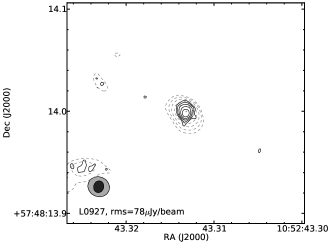
Figure 21: (Continued)

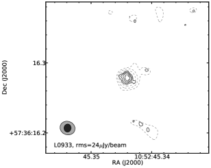
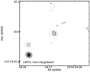
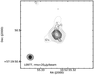
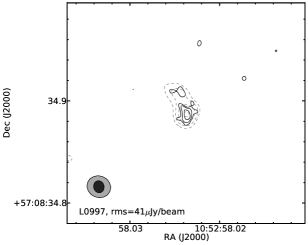
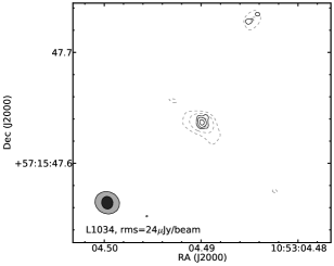
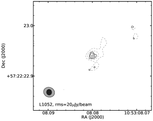
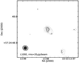
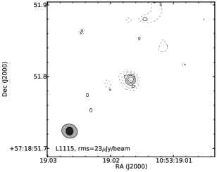
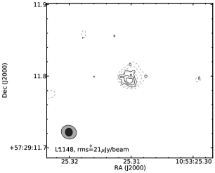
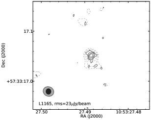
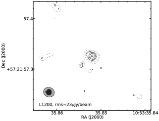
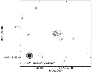
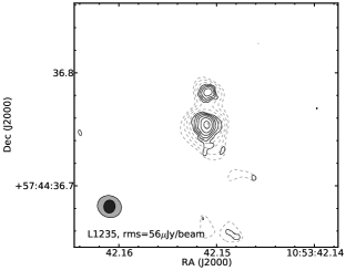
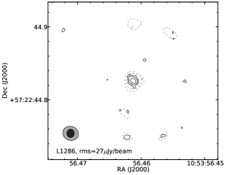
Figure 21: (Continued)

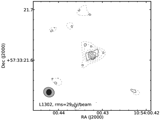
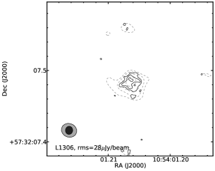
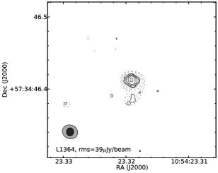
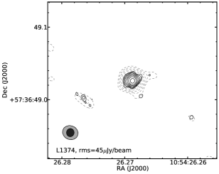
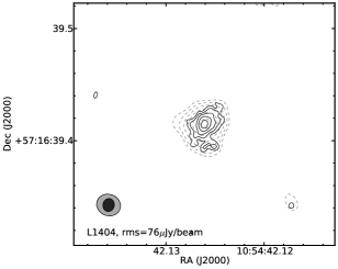
Figure 21: (Continued)

Figure 22: (Continued)

Figure 22: (Continued)

Figure 22: (Continued)

Figure 22: (Continued)