X-ray Emission from Strongly Asymmetric Circumstellar Material in the Remnant of Kepler’s Supernova

Abstract

Kepler’s supernova remnant resulted from a thermonuclear explosion, but is interacting with circumstellar material (CSM) lost from the progenitor system. We describe a statistical technique for isolating X-ray emission due to CSM from that due to shocked ejecta. Shocked CSM coincides well in position with 24 $\mu$m emission seen by Spitzer. We find most CSM to be distributed along the bright north rim, but substantial concentrations are also found projected against the center of the remnant, roughly along a diameter with position angle $\sim 100^{\circ}$. We interpret this as evidence for a disk distribution of CSM before the SN, with the line of sight to the observer roughly in the disk plane. We present 2-D hydrodynamic simulations of this scenario, in qualitative agreement with the observed CSM morphology. Our observations require Kepler to have originated in a close binary system with an AGB star companion.

1 Introduction

The remnant of Kepler’s supernova of 1604 (“Kepler” henceforth) has defied classification since its optical recovery in 1943 (Baade 1943), because of its awkward combination of clear evidence for dense circumstellar material (originally identified through an optical spectrum indicating enhanced N; Minkowski 1943), suggesting a core-collapse supernova, and light curve and location (470 kpc above the Galactic plane, for a distance of 4 kpc; Sankrit et al. 2005) indicating a Type Ia origin. X-ray studies with ASCA indicated a large mass of Fe (Kinugasa & Tsunemi 1999), and finally detailed X-ray studies with Chandra (Reynolds et al. 2007; Patnaude et al. 2012) showed conclusively that the event must have been a thermonuclear explosion (though its spectrum at maximum light may or may not have resembled a traditional Ia event).

But the evidence for circumstellar material (CSM) has not gone away. Since the question of the progenitor systems of SNe Ia is unsettled at this time, characterization of the CSM is of great importance. Observations of Type Ia supernovae consistently fail to show evidence for CSM (except in rare cases such as 2002ic, Hamuy et al. 2003, and 2005gj, Aldering et al. 2006), a finding used as evidence in favor of binary white-dwarf progenitor systems (double-degenerate, DD). Single-degenerate (SD) scenarios may involve either a main-sequence or an evolved companion (see, for example, Branch 1995; Hillebrandt & Niemeyer 2000), but searches for a surviving companion have for the most part been negative (e.g., Schaefer & Pagnotta 2012). Just as finding a companion would demand a SD progenitor, identifying CSM in a Type Ia system requires an SD scenario. However, various possibilities for the companion star are still possible. The most likely suggestion is an evolved star with a slow and massive wind (Velázquez et al. 2006; Blair et al. 2007; Chiotellis, Schure, & Vink 2012; Williams et al. 2012), i.e., an Asymptotic Giant Branch (AGB) star. In a close binary, such a star would be likely to produce an asymmetric wind, primarily in the orbital plane. Thus characterizing the amount and spatial distribution of CSM in the remnant of a Type Ia supernova has important implications for the nature of Type Ia progenitors. Here we focus on the spatial distribution of CSM, which we identify using a powerful statistical technique applied to the long Chandra observation of Kepler.

The excess of nitrogen in optical observations suggests mass loss from an evolved star. Various authors have performed hydrodynamic modeling of a system with substantial mass loss moving through the ISM with speeds of hundreds of km s^-1 (Borkowski et al. 1992; Velázquez et al. 2006; Chiotellis et al. 2012). This modeling is able to describe the observed dense shell to the north, but in these cases the wind was assumed to be isotropic. We shall show that our spatial localization of CSM requires an asymmetric wind.

2 Observations

Kepler was observed for 741 ks with the Chandra X-ray Observatory ACIS-S CCD camera (S3 chip) between April and July 2006. Data were processed using CIAO v3.4 and calibrated using CALDB v3.1.0. A large background region to the north of the remnant (covering most of the remaining area on the S3 chip) was used for all spectra. Spectral analysis was performed with XSPEC v.12 (Arnaud, 1996). We used the nonequilibrium-ionization (NEI) v2.0 thermal models, based on the APEC/APED spectral codes (Smith et al., 2001) and augmented by the addition of inner-shell processes (Badenes et al., 2006). There are a total of about $3\times 10^{7}$ source counts, with fewer than 3% background (though some of those may be dust-scattered source photons).

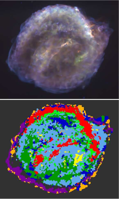
Figure 1: Top: Merged image between 0.3 and 8 keV (Reynolds et al. 2007). Red: 0.3 – 0.72 keV; green, 0.72 – 1.7 keV; blue, 1.7 – 8 keV. All three images were smoothed using platelet smoothing (Willett, 2007). Image size is $4\farcm 7\times 3\farcm 9$. Bottom: Division of Kepler into clusters (regions of similar spectral character). Colors are arbitrary. Region R (red) contains the bulk of the CSM, while purple (P) is dominated by synchrotron emission. Most of the rest is ejecta. See text for further details.

3 Gaussian Mixture decomposition

Our earlier study (Reynolds et al. 2007) showed that spectral variations occur over arcsecond scales, too small for full spectra of individual regions to have adequate statistics. This also means that simple imaging in different spectral bands is incapable of producing quantitative information characterizing regions of different spectral character. In order to concentrate regions with similar spectra for detailed spectral analysis, we instead collect regions of similar spectral character by describing each with four broad-band colors, and clustering them in a four-dimensional color space using a collection of Gaussian probability distributions (clusters). (Such a probabilistic description of multi-dimensional data is known in the literature as a Gaussian mixture model.) The clusters are now of much higher signal-to-noise than individual small regions (selected by eye, for instance, as in Reynolds et al. 2007), and were selected with objective criteria. Gaussian mixture models are well-known in many areas of science, and are becoming more widely used for a variety of applications in astrophysics (e.g., Shang & Oh 2012; Lee et al. 2012; Hurley et al. 2012).

The integrated spectrum of Kepler is dominated by ejecta emission from Fe, Si, and S, while O and Mg are expected to be primarily found in CSM. We therefore selected spectral bands to feature the oxygen Ly$\alpha$ line (0.3 to 0.72 keV), the iron L shell region (0.72 to 1.3 keV), the magnesium K$\alpha$ line (1.3 keV to 1.5 keV), and the silicon and sulfur K$\alpha$ lines (combined because of similar characteristics and behavior in the spectrum: 1.7 to 2.1 keV and 2.3 to 2.7 keV respectively). Other elements can contribute in these bands, for instance Ne K$\alpha$ and Ly$\alpha$ in the Fe L region, but the integrated spectra show that these contributions are less significant. Each of the previous energy bands was divided by the flux in unused energy bands (1.5 to 1.7, 2.1 to 2.3, and 2.7 to 7.0 keV), so that the entire spectral range was used. This gave the best signal-to-noise ratio for those fluxes, but at the cost of including some line emission in the quasi-continuum bands. However, the quasi-continuum is broad enough to allow maximum contrast with the line features we chose to highlight. (Insisting on using a more line-free continuum, such as 4–6 keV, has two drawbacks: first, since far fewer counts are present there, the ratios we seek to classify would have much higher statistical noise; and second, one cluster in particular that we identify, that of synchrotron emission, is actually less evident in 4–6 keV emission than in broader bands.) The strong contrast in the clusters we identify, as seen in Figure 2, shows that we are not unduly hampered by the presence of some line emission in our quasi-continuum band.

We divided the observation into about 5000 segments with sizes adjusted to produce comparable numbers of counts (about 6000 each), and extracted the counts in the four line bands plus continuum for each. We then produced a four-dimensional scatterplot of all 5000 segments using the logs of normalized band counts. Using the publicly available software package mclust written in R (Fraley et al. 2012), we decomposed the four-dimensional distribution into several four-dimensional Gaussian clusters, each characterized by at most 15 parameters: its weight relative to other clusters, a center in each of four coordinates, and a (symmetric) $4\times 4$ covariance matrix. The number of Gaussians required was found by the algorithm using the Bayesian Information Criterion (BIC), which was optimized for nine clusters. However, the clusters corresponding to CSM emerged clearly for any total number of clusters between five and ten.

In the Gaussian mixture model, each segment is associated with a set of probabilities of belonging to each of the clusters. We will from now on refer to each cluster more narrowly as a set of segments that have the highest probability of belonging to this cluster. Figure 1 shows the spatial distribution of the segments making up each cluster. The tendency of segments of similar spectral character to form contiguous regions gives us confidence in the method. Summed spectra of all segments in several clusters are shown in Figure 2. We shall refer to the clusters by abbreviations for their colors in Fig. 1: R (red), O (orange), Y (yellow), LG (light green), DG (dark green), LB (light blue), DB (dark blue), P (purple) and B (black). The values of the count ratios that define the center of each cluster are given in Table 1.

The clusters containing the most prominent emission in the ejecta-dominated bands are regions LB, DG, LG, and Y. Figure 2 (top) shows region LG contrasted with CSM-dominated regions, while the others are shown in Figure 2 (bottom). Each of their spectra contained similar Fe L, Si K$\alpha$ and K$\beta$, S K$\alpha$ and K$\beta$, Ar K$\alpha$, and Ca K$\alpha$ features with the exception of region DG, whose features were much more muted. Region LG is the brightest of the four, because of its close proximity to the bright north rim. Region Y contains the highest concentration of iron in the remnant in a localized patch. The outer ejecta knots containing lighter materials are contained primarily in region O as seen by the very high silicon to iron ratios within the spectrum. Synchrotron radiation is represented by region P as the spectrum is almost featureless. Regions R, DB, and B contain the clearest Mg feature, suggesting CSM. These regions are compared in the two spectral plots of Figure 2. The vast majority of the CSM is contained within region R. Confirmation of this separation’s effectiveness is evidenced by comparing region R to the Spitzer 24 $\mu$m image of SN1604 (Fig. 3; Blair et al. 2007) which highlights the heated dust that is evidence of CSM. The two images are extremely similar.

We can examine this issue more closely. Figure 2 shows the integrated spectrum of region R (red, top), along with region LG (green, second from top), west-central portion of region R (third from top) with local background subtracted, and finally the spectrum of a small knot reproduced from Reynolds et al. (2007), also with a local background subtracted (bottom). The west-central spectrum also shows the CSM component from a multicomponent fit (dotted line; see below). The contrast between regions R and LG is evident: the different peak energies result from a higher contribution from Ne in region R and from Fe L in region LG. Region R also shows a feature between 0.6 and 0.7 keV, O Ly $\alpha$, which is more obvious in the lower two spectra. The obviously greater prominence of both O and Mg in all of Region R (especially in the central emission) and the smaller contribution from Fe confirm the association of those regions with CSM.

While we might expect CSM to be found around the outer edge of the SNR, its presence across the central region is striking. Blair, Long, & Vancura (1991) first pointed out the presence of nonradiative shocks there, indicating partially neutral upstream material. They found that knots in the eastern part of the central emission showed redshifts of order 500 km s^-1 while those in the western part were blueshifted by about $-600$ km s^-1, indicating that the former were on the far side and the latter on the near side, projected against the center. Our completely independent analysis locates the same regions, and we adopt the same interpretation.

4 Quantitative analysis of CSM

The integrated spectrum of Region R clearly shows distinctive features consistent with its identification as CSM. Ideally, we would use oxygen as a tracer of CSM, as relatively little O is present in most SN Ia models (e.g., Maeda et al. 2010). However, while an inflection at the energy of O Ly$\alpha$ (0.65 keV) can be seen in some of the spectra of Figure 2, the substantial absorbing column density makes quantitative analysis difficult. The clearest signal of an element not expected to be synthesized in much quantity in a SN Ia (e.g., Maeda et al. 2010) comes from Mg K$\alpha$ (1.34 keV), with the absence of Mg Ly$\alpha$ (1.47 keV) as a constraint. The regions we identify as CSM have weak, but well-isolated and easily characterized, emission features for Mg K$\alpha$, and we use that line to quantify CSM (Figure 3, center).

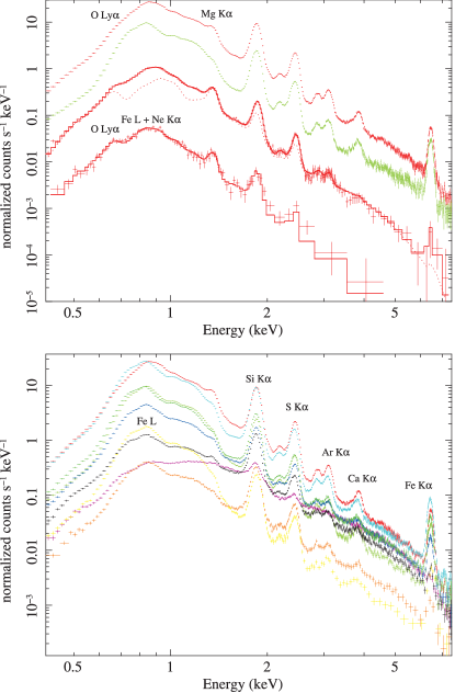
Figure 2: Top: Spectra of primary CSM regions compared to ejecta-dominated Region LG. Top: Total of Region R. Next: Region LG. Third: West central part of Region R, with local background subtracted; dotted curve is the CSM component from the multicomponent spectral fit described in the text. Bottom: Small knot in central region with local background subtracted, reproduced from Reynolds et al. (2007). Notice the clear O and Mg features in all three CSM spectra. Bottom: Spectra of primary ejecta regions compared to the synchrotron region and Region R. Comparable in strength to Region R is Region LB; note the difference in shape near the peak, due to Fe L dominance of Region LB. In order of decreasing brightness at 1 keV: Regions LG, DG, DB, Y, B, P (synchrotron) and O.

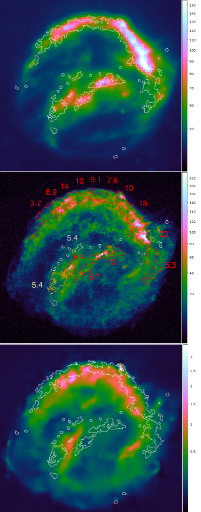
Figure 3: Top: Region R (contours) plus an IR-bright central subregion of Region LG superposed on the 24 $\mu$m Spitzer image (Blair et al. 2007). Color scale is in MJy sr^-1. Middle: Soft X-ray image (ct pixel^-1 in 0.3 – 0.72 keV) from Chandra, with contours of subregions of CSM-dominated Region R (contours) plus the IR-bright central LG subregion. Numbers: Mg line-strength surface brightnesses (units: $10^{-8}$ photons cm^-2 s^-1 arcsec ^-2). Bottom: Region R contours superposed on a smoothed image from 6.2 to 6.8 keV (Fe K). The IR-bright LG subregion overlaps with the peak of central Fe K emission. Note the poor correlation between strong Fe emission and CSM, especially in the west-central region.

We subdivided the CSM-dominated region R into 14 subregions, and extracted spectra from each. We subtracted background from a large region to the north of the remnant. Spectra were fitted with two Gaussians for the two lines and power-law model for the continuum, between 1.2 and 1.6 keV, yielding line strengths. The Ly$\alpha$ feature was often negligible. For each subregion, we calculated the line-strength surface brightness (ph cm^-2 s^-1 arcsec^-2). These values are shown in Figure 3 (center).

The west-central portion of region R, with a surface area of 410 arcsec² and a Mg K$\alpha$ flux of $4.2\times 10^{-5}$ ph cm^-2 s^-1, rivals the bright northern rim in Mg K$\alpha$ surface brightness. In order to learn more about its plasma properties, we modeled its spectrum with a simple plane shock (vpshock model in XSPEC). As in Reynolds et al. (2007), we assumed an absorbing column density $N_{H}=5.2\times 10^{21}$ cm^-2. Wilms et al. (2000) solar abundances were adopted for all elements except for N (fixed to $3\times$ solar) and Ne and Mg (that we allowed to vary in the fitting process). The ejecta contribution was modeled by a pure Fe, NEI v1.1 vpshock model plus a separate single-ionization-timescale model vnei containing intermediate-mass (Si, S, Ar, and Ca) elements. (We also added a Gaussian line at 0.73 keV in order to account for missing Fe lines in the NEI v1.1 atomic code.) Ejecta contribute to the spectrum mostly in Fe L- and K-shell lines, and in K$\alpha$ lines of Si, S, and Ar (see Fig. 2). The temperature and ionization age of the dominant CSM component are 1.2 keV and $1.1\times 10^{11}$ cm^-3 s, and the fitted Ne and Mg abundances are near solar (0.7 and 1.2, respectively). This component is plotted as the dotted curve in Figure 2; it accounts for almost all the emission except for obvious Fe L and K emission. Fits with a more elaborate vnpshock model with unequal ion and electron temperatures reproduce these results. For an assumed shock velocity of $\sim 1500$ km s^-1 (corresponding to the mean temperature of 2.7 keV), typical for Balmer-dominated shocks in Kepler’s SNR (Blair et al. 1991), electrons are heated first to 0.8 keV at the shock front, and then gain energy through Coulomb collision with ions. Average properties of the shocked CSM in the west-central portion of region R appear typical of Kepler as a whole, although its emission measure of $0.32M_{\odot}d_{4}^{2}$ cm^-3 is only a small fraction of the total emission measure of $\sim 10M_{\odot}d_{4}^{2}$ cm^-3 (see Blair et al. 2007 for a discussion of the CSM plasma properties as derived from the spatially-integrated XMM-Newton RGS spectrum). Blue-shifted optical emission found at this location by Blair et al. (1991) indicates that this material was expelled toward us by the SN progenitor. We also performed a spectral analysis of the adjacent central portion of region R farther south and east that contains red-shifted optical emission from material expelled away from us by the SN progenitor. We found the same Ne and Mg abundances there but a slightly higher temperature of 1.5 keV, a somewhat shorter ionization age of $7.1\times 10^{10}$ cm^-3 s, and a significantly smaller emission measure of $0.078M_{\odot}d_{4}^{2}$ cm^-3. These results may be interpreted as a modest density effect, where the blue-shifted west-central portion of the CSM is somewhat denser than the red-shifted portion farther south and east.

Although the spatial correlation between region R and the IR emission is reasonably good, it is far from perfect. One reason for this might be superposition of ejecta and CSM along the line of sight. We examined X-ray spectra at an IR bright east-central location (see Fig. 3) that is part of the ejecta-dominated LG region. While the Fe L-shell emission dominates, a strong Mg K$\alpha$ line is also present, with a surface brightness as high as found in central portions of region R. An image in the 6.2 – 6.8 keV energy range shows a prominent Fe K$\alpha$-emitting filament intersecting the central CSM band at this location (Fig. 3). Apparently, both the CSM and Fe-rich ejecta contribute significantly to the X-ray spectrum of this region. They may even arise from physically adjacent regions, as the collision of Fe-rich ejecta with denser than average CSM might be expected to enhance Fe L- and K-shell emission. But the overall spatial correlation between Fe-rich ejecta (as traced by the Fe K$\alpha$ emission) and the CSM is quite poor in the central regions of the remnant, presumably because of the asymmetric distribution of Fe within the SN ejecta.

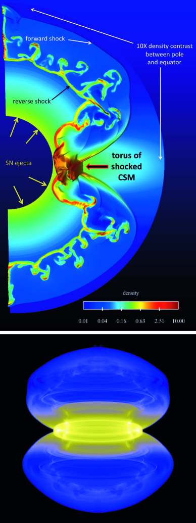
Figure 4: Top: Hydrodynamic simulation of density as a blast wave encounters an equatorial wind. At this time, the swept-up mass is comparable to the ejected mass of $1.4M_{\odot}$. The wind speed has been neglected compared to the blast-wave speed. Bottom: Line-of-sight integration of density squared from the hydrodynamic simulation. The symmetry axis is tilted out of the sky plane by 10^∘.

5 Hydrodynamic simulations

The presence of the band of CSM across the center of Kepler (echoed by the presence of nonradiative H$\alpha$ emission) indicates that this material is seen in projection in front and in back of the remnant. Such a morphology could result from a pre-SN CSM distribution that is predominantly disk-like, as expected for mass loss from AGB stars (see Section 6 below for references), with the line of sight roughly in the plane of the disk. To examine this possibility more closely, we performed 2-D hydrodynamic simulations of an ejecta-driven blast wave expanding into an azimuthally varying stellar wind, with density varying by a factor of 10 from pole to equator. Half the wind mass is within $10^{\circ}$ of the equator. We ignored the wind speed as it is a few tens of km s^-1, negligible compared to the blast-wave speed. We did not attempt to model the north-south density gradient (Blair et al. 2007), presumably the result of system motion to the north or northwest (Bandiera 1987). We modeled the SN ejecta with an exponential profile appropriate for Type Ia explosions (Dwarkadas & Chevalier 1998). We used the well-tested code VH-1, a conservative, finite-volume code for evolving the Euler equations describing an ideal, compressible gas. The details of the numerical simulation follow the procedure described in Warren & Blondin (2012).

Figure 4 shows a stage at which the swept-up CSM mass is about equal to the ejected mass ($1.4M_{\odot}$). A torus of shocked CSM occupies the equatorial plane. The lower panel of Figure 4 shows a 3-D projection of the model, integrating the square of the density (proportional to emission measure) along lines of sight, with the symmetry axis tilted by $10^{\circ}$ to the plane of the sky. The result is an incomplete bar of shocked CSM across the remnant center as observed, whose radius is about half that of the extent to the north and south, in rough agreement with the central bar of CSM we observe. While the simulation is only suggestive, it indicates that more detailed study of such a model may lead to an improved understanding of Kepler’s dynamics.

6 Discussion

Our observations of CSM toward the center of Kepler are naturally explained by a disk seen edge-on, while the bright northern rim results from northward motion of the system (Bandiera 1987). Such an asymmetric distribution of CSM is expected from a binary system, where an equatorial disk of enhanced mass loss is likely. Inferences of CSM around at least a few Type Ia SNe continue to accumulate (e.g., SN 2008J; Taddia et al. 2012; PTF11kx; Dilday et al. 2012). In particular, Dilday et al. (2012) infer a substantially asymmetric CSM distribution, suggesting a symbiotic binary progenitor system with mass loss concentrated in the orbital plane. In an SD model for Kepler, as required by the CSM, we expect the companion to have been an AGB star. Some AGB stars show dense envelopes accessible to study through molecular emission such as CO; on scales of $10^{\prime\prime}-20^{\prime\prime}$, the emission is relatively symmetric (Neri et al. 1998). A few systems seem to require asymmetry, though the incomplete sampling of the 3-element IRAM interferometer used by Neri et al. (1998) make detailed imaging impossible. Additional observational evidence for asymmetric winds from evolved stars is presented by Chiu et al. (2009) and Huggins (2007). On theoretical grounds, we expect that the winds from AGB stars in detached binaries can, through gravitational focusing by the companion, produce highly asymmetric CSM, with density contrasts of 10 or more found in numerical simulations by Mastrodemos & Morris (1999) and characterized by Huggins, Mauron, & Wirth (2009). Politano & Taam (2011) find that several percent of AGB systems should show such strong asymmetries. In a particular case, 3D simulations of RS Oph (Walder, Folini, & Shore 2008) show very large equator-to-pole density variations on the scale of the orbital separation, averaging to factors of 2 – 3 on much larger scales. These simulations do not consider the possibility of a wind from the white-dwarf companion (Hachisu et al. 1996), which would tend to evacuate material perpendicular to the plane of the disk and enhance the equator-to-pole density contrast.

The distribution of strong Fe emission in Kepler is worthy of note. Most Type Ia SN models produce highly stratified ejecta, so most Fe should be in the remnant interior. Where the ejecta impact the dense wind in the equatorial plane, then, one might expect enhanced Fe emission – so in a plane roughly coincident with the plane of central CSM. This does not appear to be the case. Fe K$\alpha$ emission toward Kepler’s interior is asymmetrically distributed, with one patch near the east-central CSM emission, but less near the west-central CSM. We speculate that one cause of Fe asymmetry might be the “shadow” in Fe cast by the companion star, blocking the ejection of material in that direction. Pan et al. (2012) estimate that a RG companion can shadow up to 18% of the solid angle from the ejecta of a Type Ia SN, while García-Senz et al. (2012) show that morphological effects of a companion’s shadow can survive for hundreds of years. Further study of Fe in particular in Kepler will allow us to examine this possibility in more detail.

7 Conclusions

We have used Gaussian mixture decompositions of multicolor X-ray spectral data from the long Chandra observation of Kepler’s supernova remnant to identify and characterize regions of shocked circumstellar material, as distinct from the ejecta that dominate the integrated spectrum. We find that shocked CSM is co-located with both nonradiative shocks identified by H$\alpha$ emission, and with 24 $\mu$m dust continuum emission seen with Spitzer. We suggest that the central band of CSM is the remnant of a circumstellar disk seen edge-on. Our 2-D hydrodynamic simulation shows that a blast wave encountering an equatorial wind from a companion can naturally produce this morphology. The asymmetry we observe requires a binary progenitor system in which the donor is an evolved (AGB) star.

Table 1: Cluster Centers

Energy Band	B	P	DB	LB	DG	LG	Y	O	R
O	0.89	0.73	1.01	1.13	1.1	1.11	1.23	0.87	1.05
Fe	1.2	1.07	1.35	1.49	1.44	1.47	1.68	1.31	1.39
Mg	0.9	0.87	0.96	1.02	0.97	1.03	1.07	0.89	1.05
Si/S	1.1	0.97	1.11	1.19	1.16	1.17	1.19	1.13	1.14

Note. — Entries are the logarithms of ratios of counts in the four energy bands to continuum at the centers of each of the nine clusters identified by the Gaussian Mixture Method. Bands are described more fully in the text.

References

- Aldering et al. (2006) Aldering, G., et al. 2006, ApJ, 650, 510
- Arnaud (1996) Arnaud, K.A., in ASP Conf.Ser.101, Astronomical Data Analysis and Systems V, ed. G. Jacoby & J. Barnes (San Francisco: ASP), 17
- Baade (1943) Baade, W. 1943, ApJ, 97, 119
- Badenes et al. (2006) Badenes, C., et al. 2006, ApJ, 645, 1373
- Bandiera (1987) Bandiera, R. 1987, ApJ, 319, 885
- Blair, Long, & Vancura (1991) Blair, W.P., Long, K.S., & Vancura, O. 1991, ApJ, 366, 484
- Blair et al. (2007) Blair, W.P., et al. 2007, ApJ, 662, 998
- Branch et al. (1995) Branch, D., et al. “In Search of the Progenitors of Type Ia Supernovae.” 1995, PASP, 107, 1019–1029.
- Chiotellis, Schure, & Vink (2012) Chiotellis, A., Schure, K.M., & Vink, J. 2012, A&A, 537, A139
- Chiu et al. (2009) Chiu P.-J., Hoang C.-T., Dinh-V-Trung L. J., Kwok S., Hirano N., Muthu C. 2006, ApJ, 645, 605
- Dilday et al. (2012) Dilday, B., et al. 2012, Science, 337, 942
- Dwarkadas & Chevalier (1998) Dwarkadas, V., & Chevalier, R.A. 1998, ApJ, 497, 807
- Fraley et al. (2012) Fraley, C., Raftery, A.E., Murphy, T.B., & Scrucca, L. 2012, Technical Report 597, Dept. of Statistics, U. Washington (available at http://www.stat.washington.edu/mclust/)
- García-Senz, Badenes, & Serichol (2012) García-Senz, D., Badenes, C., & Serichol, N. 2012, ApJ, 745:75
- Hachisu, Kato, & Nomoto (1996) Hachisu, I., Kato, M., & Nomoto, K. 1996, ApJ, 470, L97
- Hamuy et al. (2003) Hamuy, M., et al. 2003, Nature, 424, 651
- Hillebrandt & Niemeyer (2000) Hillebrandt, W., & Niemeyer, J.C. 2000, ARA&A, 38, 191
- Huggins (2007) Huggins, P.J. 2007, ApJ, 663, 342
- Huggins, Mauron, & Wirth (2009) Huggins, P.J., Mauron, N., & Wirth, E.A. 2009, MNRAS, 396, 1805
- Hurley et al. (2012) Hurley, P.D., Oliver, S., Farrah, D., Wang, L., & Efstathiou, A. 2012, MNRAS, 424, 2069
- Kinugasa & Tsunemi (1999) Kinugasa, K., & Tsunemi, H. 1999, PASJ, 51, 239
- Lee et al. (2012) Lee, K.J., Guillemot, L., Yue, Y.L., Kramer, M., & Champion, D.J. 2012, 424, 2832
- Maeda et al. (2010) Maeda, K., Röpke, F.K., Fink, M., Hillebrandt, W., Travaglio, C., & Thielemann, F.-K. 2010, ApJ, 712, 624
- Mastrodemos & Morris (1999) Mastrodemos, N., & Morris, M. 1999, ApJ, 523, 357
- Minkowski (1943) Minkowski, R. 1943, ApJ, 97, 128
- Neri et al. (1998) Neri, R., et al. 1998, A&AS, 130, 1
- Pan, Ricker, & Tam (2012) Pan, K.-C., Ricker, P.M., & Taam, R.E. 2012, ApJ, 750:151
- Patnaude et al. (2012) Patnaude, D.J., Badenes, C., Park, S., & Laming, J.M. 2012, ApJ, 756, 6P
- Politano & Taam (2011) Politano, M, & Taam, R.E. 2011, ApJ, 741, 5
- Reynolds et al. (2007) Reynolds, S.P., et al. 2007, ApJ, 668, L135
- Sankrit et al. (2005) Sankrit, R., et al. 2005, ASR, 35, 1027
- Schaefer & Pagnotta (2012) Schaefer, B.E., & Pagnotta, A. 2012, Nature, 481, 164
- Shang & Oh (2012) Shang, C., & Oh, S.P. 2012, MNRAS, 426, 3435
- Smith et al. (2001) Smith, R.K., et al. 2001, ApJ, 556, L91
- Taddia et al. (2012) Taddia, F., et al. 2012, A&A, 545, L7
- Velázquez et al. (2006) Velázquez, P.F., Vigh, C.D., Reynoso, E.M., Gómez, D.O., & Schneiter, E.M. 2006, ApJ, 649, 779
- Walder, Folini, & Shore (2008) Walder, R., Folini, D., & Shore, S.N. 2008, A&A, 484, L9
- Warren & Blondin (2012) Warren, D., & Blondin, J.M. 2012, MNRAS, submitted
- Willett (2007) Willett, R. 2007, in ASP Conf.Ser.371, Statistical Challenges in Modern Astronomy IV, ed. G.J. Babu & E.D. Feigelson (San Francisco: ASP) 247
- Williams et al. (2012) Williams, B.J., et al. 2012, ApJ, 755:3
- Wilms, Allen, & McCray (2000) Wilms, J., Allen, A., & McCray, R. 2000, ApJ, 542, 914