Variational Optimization

Joe Staines and David Barber
University College London - Computer Science
Gower Street, London, WC1E 6BT - United Kingdom
Abstract

We discuss a general technique that can be used to form a differentiable bound on the optima of non-differentiable or discrete objective functions. We form a unified description of these methods and consider under which circumstances the bound is concave. In particular we consider two concrete applications of the method, namely sparse learning and support vector classification.

1 Optimization by Variational Bounding

We consider the general problem of function maximization, maxxโกfโ€‹(x)subscript๐‘ฅ๐‘“๐‘ฅ\displaystyle\max_{x}f({x}) for vector x๐‘ฅx. When f๐‘“f is differentiable and x๐‘ฅx continuous, optimization methods that use gradient information are typically preferred over non-gradient based approaches since they are able to take advantage of a locally optimal direction in which to search. However, in the case that f๐‘“f is not differentiable or x๐‘ฅx is discrete, gradient based approaches are not directly applicable. In that case, alternatives such as relaxation, coordinate-wise optimization and stochastic approaches are popular [1]. Our interest is to discuss another general class of methods that yield differentiable surrogate objectives for discrete x๐‘ฅx or non-differentiable f๐‘“f. The Variational Optimization (VO) approach is based on the simple bound111Note that this provides a bound on the optimum of fโ€‹(x)๐‘“๐‘ฅf(x), not necessarily on fโ€‹(x)๐‘“๐‘ฅf(x) itself.

fโˆ—=maxxโˆˆ๐’žโกfโ€‹(x)โ‰ฅ<fโ€‹(x)>pโ€‹(x|ฮธ)โ‰กEโ€‹(ฮธ)superscript๐‘“subscript๐‘ฅ๐’ž๐‘“๐‘ฅsubscriptexpectation๐‘“๐‘ฅ๐‘conditional๐‘ฅ๐œƒ๐ธ๐œƒf^{*}=\max_{x\in\mathcal{C}}f({x})\geq\big{<}f(x)\big{>}_{p({x}|\theta)}\equiv E(\theta) (1)

where โŸจโ‹…โŸฉpsubscriptdelimited-โŸจโŸฉโ‹…๐‘\left\langle{\cdot}\right\rangle_{p} denotes expectation with respect to the distribution p๐‘p defined over the solution space ๐’ž๐’ž\mathcal{C}. The parameters ฮธ๐œƒ\theta of the distribution pโ€‹(x|ฮธ)๐‘conditional๐‘ฅ๐œƒp(x|\theta) can then be adjusted to maximize the lower bound Eโ€‹(ฮธ)๐ธ๐œƒE(\theta). This bound can be trivially made tight provided the distribution pโ€‹(x|ฮธ)๐‘conditional๐‘ฅ๐œƒp(x|\theta) is flexible enough to allow all its mass to be placed in the optimal state xโˆ—=argโกmaxxโกfโ€‹(x)superscript๐‘ฅsubscript๐‘ฅ๐‘“๐‘ฅ{x}^{*}=\arg\max_{x}f(x).

Under mild restrictions, the bound is differentiable, see section(1.1), and the bound is a smooth alternative objective function (see also section(4.1) on the relation to โ€˜smoothingโ€™ methods). The degree of smoothness (and the deviation from the original objective) increases as the dispersion of the variational distribution increases. In section(1.2) we give sufficient conditions for the variational bound to be concave. The purpose of this paper is to demonstrate the ease with which VO can be applied and to discuss its merits as a general way to construct a smooth alternative objective.

1.1 Differentiability of the variational objective

When fโ€‹(x)๐‘“๐‘ฅf(x) is not differentiable, under weak conditions Eโ€‹(ฮธ)๐ธ๐œƒE(\theta) can be made differentiable. The gradient of Eโ€‹(ฮธ)๐ธ๐œƒE(\theta) is given by

โˆ‚Eโˆ‚ฮธ=โˆ‚โˆ‚ฮธโ€‹โˆซ๐’žfโ€‹(x)โ€‹pโ€‹(x|ฮธ)โ€‹๐‘‘x.๐ธ๐œƒ๐œƒsubscript๐’ž๐‘“๐‘ฅ๐‘conditional๐‘ฅ๐œƒdifferential-d๐‘ฅ\frac{\partial E}{\partial\theta}=\frac{\partial}{\partial\theta}\int_{\mathcal{C}}f(x)p(x|\theta)dx. (2)

We can bring the differential under the integral sign provided:

(i) fโ€‹(x)โ€‹pโ€‹(x|ฮธ)๐‘“๐‘ฅ๐‘conditional๐‘ฅ๐œƒf({x})p(x|\theta) is Lebesgue integrable and differentiable with respect to ฮธ๐œƒ\theta

(ii) there exists an integrable function F:๐’žโ†’โ„:๐นโ†’๐’žโ„F:\mathcal{C}\rightarrow\mathbbm{R} such that, for all ฮธ๐œƒ\theta,

|โˆ‚โˆ‚ฮธf(x)p(x|ฮธ)|<F(x)\left|\frac{\partial}{\partial\theta}f({x})p(x|\theta)\right|<F(x) (3)

These weak conditions mean that for a large-class of problems in which f๐‘“f is non-differentiable or x๐‘ฅx discrete, the bound Eโ€‹(ฮธ)๐ธ๐œƒE(\theta) is differentiable with respect to the parameters ฮธ๐œƒ\theta. For example, consider the non-differentiable objective fโ€‹(x)โ‰ก๐•€โ€‹[xโ‰ฅ0]๐‘“๐‘ฅ๐•€delimited-[]๐‘ฅ0f(x)\equiv\mathbb{I}\left[{x\geq 0}\right] with x๐‘ฅx normally distributed with mean 00 and unit variance, pโ€‹(x|ฮธ)=๐’ฉโ€‹(xโ€‹ฮธ,1)๐‘conditional๐‘ฅ๐œƒ๐’ฉ๐‘ฅ๐œƒ1p(x|\theta)={\cal{N}}\left({x\thinspace\vline\thinspace\theta,1}\right). Then โˆ‚Eโˆ‚ฮธ=expโก(โˆ’ฮธ2/2)/2โ€‹ฯ€๐ธ๐œƒsuperscript๐œƒ222๐œ‹\frac{\partial E}{\partial\theta}=\exp(-\theta^{2}/2)/\sqrt{2\pi}.

1.2 Concavity of the variational bound

Here we consider the special case of continuous x๐‘ฅx and non-differentiable fโ€‹(x)๐‘“๐‘ฅf(x) and describe conditions which are sufficient for Eโ€‹(ฮธ)๐ธ๐œƒE(\theta) to be concave in ฮธ๐œƒ\theta222The variational objective Eโ€‹(ฮธ)=โŸจfโ€‹(x)โŸฉqโ€‹(x|ฮธ)๐ธ๐œƒsubscriptdelimited-โŸจโŸฉ๐‘“๐‘ฅ๐‘žconditional๐‘ฅ๐œƒE(\theta)=\langle f(x)\rangle_{q(x|\theta)} is bounded above and below by the maximum and minimum of fโ€‹(x)๐‘“๐‘ฅf(x). Where the minimum is finite then, Eโ€‹(ฮธ)๐ธ๐œƒE(\theta) cannot be strictly concave over all parameter space ฮธโˆˆโ„N๐œƒsuperscriptโ„๐‘\theta\in\mathbb{R}^{N}. This prevents us from forming strictly convex problems for fully unconstrained ฮธ๐œƒ\theta whenever f๐‘“f has finite minimum. However, even in this case, the bound may be quasi-concave (uni-modal).. To do this we take advantage of a recent result by [2] to prove the concavity of a Kullback-Leibler based variational approximation for generalized linear models. We first introduce the general concept of an expectation affine distribution.

  • Definition

    (Expectation affine) A distribution pโ€‹(x|ฮธ)๐‘conditional๐‘ฅ๐œƒp(x|\theta) is expectation affine if, for linear functions ฮฑ๐›ผ\alpha, ฮฒ๐›ฝ\beta, distribution qโ€‹(z)๐‘ž๐‘งq(z) and function f๐‘“f,

    <fโ€‹(x)>pโ€‹(x|ฮธ)=<fโ€‹(ฮฑโ€‹(ฮธ)โ€‹z+ฮฒโ€‹(ฮธ))>qโ€‹(z)subscriptexpectation๐‘“๐‘ฅ๐‘conditional๐‘ฅ๐œƒsubscriptexpectation๐‘“๐›ผ๐œƒ๐‘ง๐›ฝ๐œƒ๐‘ž๐‘ง\big{<}f(x)\big{>}_{p(x|\theta)}=\Big{<}f\big{(}\alpha(\theta)z+\beta(\theta)\big{)}\Big{>}_{q(z)} (4)
Theorem 1

Let fโ€‹(x)๐‘“๐‘ฅf(x) be a concave function and pโ€‹(x|ฮธ)๐‘conditional๐‘ฅ๐œƒp(x|\theta) an expectation affine distribution. Then Eโ€‹(ฮธ)โ‰กโŸจfโ€‹(x)โŸฉpโ€‹(x|ฮธ)๐ธ๐œƒsubscriptdelimited-โŸจโŸฉ๐‘“๐‘ฅ๐‘conditional๐‘ฅ๐œƒE(\theta)\equiv\left\langle{f(x)}\right\rangle_{p(x|\theta)} is concave in ฮธ๐œƒ\theta.

  • Proof

    Defining ฮป~โ‰ก1โˆ’ฮป~๐œ†1๐œ†\tilde{\lambda}\equiv 1-\lambda and using the fact that p๐‘p is expectation affine,

    Eโ€‹(ฮปโ€‹ฮธ1+ฮป~โ€‹ฮธ2)๐ธ๐œ†subscript๐œƒ1~๐œ†subscript๐œƒ2\displaystyle E(\lambda\theta_{1}+\tilde{\lambda}\theta_{2}) =<fโ€‹(ฮฑโ€‹(ฮปโ€‹ฮธ1+ฮป~โ€‹ฮธ2)โ€‹z+ฮฒโ€‹(ฮปโ€‹ฮธ1+ฮป~โ€‹ฮธ2))>qโ€‹(z)absentsubscriptexpectation๐‘“๐›ผ๐œ†subscript๐œƒ1~๐œ†subscript๐œƒ2๐‘ง๐›ฝ๐œ†subscript๐œƒ1~๐œ†subscript๐œƒ2๐‘ž๐‘ง\displaystyle=\Big{<}f\big{(}\alpha(\lambda\theta_{1}+\tilde{\lambda}\theta_{2})z+\beta(\lambda\theta_{1}+\tilde{\lambda}\theta_{2})\big{)}\Big{>}_{q(z)} (5)
    =<fโ€‹(ฮปโ€‹(ฮฑโ€‹(ฮธ1)โ€‹z+ฮฒโ€‹ฮธ1)+ฮป~โ€‹(ฮฑโ€‹(ฮธ2)โ€‹z+ฮฒโ€‹(ฮธ2)))>qโ€‹(z)absentsubscriptexpectation๐‘“๐œ†๐›ผsubscript๐œƒ1๐‘ง๐›ฝsubscript๐œƒ1~๐œ†๐›ผsubscript๐œƒ2๐‘ง๐›ฝsubscript๐œƒ2๐‘ž๐‘ง\displaystyle=\bigg{<}f\Big{(}\lambda\big{(}\alpha\left({\theta_{1}}\right)z+\beta\theta_{1}\big{)}+\tilde{\lambda}\big{(}\alpha\left({\theta_{2}}\right)z+\beta(\theta_{2})\big{)}\Big{)}\bigg{>}_{q(z)} (6)

    Since f๐‘“f is concave, then

    fโ€‹(ฮปโ€‹x1+ฮป~โ€‹x2)โ‰ฅฮปโ€‹fโ€‹(x1)+ฮป~โ€‹fโ€‹(x2)๐‘“๐œ†subscript๐‘ฅ1~๐œ†subscript๐‘ฅ2๐œ†๐‘“subscript๐‘ฅ1~๐œ†๐‘“subscript๐‘ฅ2f(\lambda x_{1}+\tilde{\lambda}x_{2})\geq\lambda f(x_{1})+\tilde{\lambda}f(x_{2}) (7)

    Hence

    Eโ€‹(ฮปโ€‹ฮธ1+ฮป~โ€‹ฮธ2)๐ธ๐œ†subscript๐œƒ1~๐œ†subscript๐œƒ2\displaystyle E(\lambda\theta_{1}+\tilde{\lambda}\theta_{2}) โ‰ฅฮปโ€‹<fโ€‹(ฮฑโ€‹(ฮธ1)โ€‹z+ฮฒโ€‹(ฮธ1))>qโ€‹(z)+ฮป~โ€‹<fโ€‹(ฮฑโ€‹(ฮธ2)โ€‹z+ฮฒโ€‹(ฮธ2))>qโ€‹(z)absent๐œ†subscriptexpectation๐‘“๐›ผsubscript๐œƒ1๐‘ง๐›ฝsubscript๐œƒ1๐‘ž๐‘ง~๐œ†subscriptexpectation๐‘“๐›ผsubscript๐œƒ2๐‘ง๐›ฝsubscript๐œƒ2๐‘ž๐‘ง\displaystyle\geq\lambda\Big{<}f\big{(}\alpha(\theta_{1})z+\beta(\theta_{1})\big{)}\Big{>}_{q(z)}+\tilde{\lambda}\Big{<}f\big{(}\alpha(\theta_{2})z+\beta(\theta_{2})\big{)}\Big{>}_{q(z)} (8)
    =ฮปโ€‹Eโ€‹(ฮธ1)+ฮป~โ€‹Eโ€‹(ฮธ2)absent๐œ†๐ธsubscript๐œƒ1~๐œ†๐ธsubscript๐œƒ2\displaystyle=\lambda E(\theta_{1})+\tilde{\lambda}E(\theta_{2}) (9)

1.2.1 Concavity for Gaussian p๐‘p

As an example, consider a multivariate Gaussian distribution pโ€‹(x|ฮผ,C)๐‘conditional๐‘ฅ๐œ‡๐ถp(x|\mu,C) with mean ฮผ๐œ‡\mu and covariance ฮฃ=Cโ€‹CTฮฃ๐ถsuperscript๐ถT\Sigma=CC^{\textsf{T}}, where C๐ถC is the Cholesky factor. Then using the change of variables z=Cโˆ’1โ€‹(xโˆ’ฮผ)๐‘งsuperscript๐ถ1๐‘ฅ๐œ‡z=C^{-1}\left({x-\mu}\right) we have

<fโ€‹(x)>pโ€‹(x|ฮผ,C)=<fโ€‹(Cโ€‹z+ฮผ)>๐’ฉโ€‹(zโ€‹โ€‰โ€‰0,I)subscriptexpectation๐‘“๐‘ฅ๐‘conditional๐‘ฅ๐œ‡๐ถsubscriptexpectation๐‘“๐ถ๐‘ง๐œ‡๐’ฉ๐‘งโ€‰โ€‰0๐ผ\big{<}f(x)\big{>}_{p\left({x|\mu,C}\right)}=\big{<}f(Cz+\mu)\big{>}_{{\cal{N}}\left({z\thinspace\vline\thinspace 0,I}\right)} (10)

That is, we can replace the average w.r.t. ๐’ฉโ€‹(xโ€‹ฮผ,ฮฃ)๐’ฉ๐‘ฅ๐œ‡ฮฃ{\cal{N}}\left({x\thinspace\vline\thinspace\mu,\Sigma}\right) by an average with respect to the standard multivariate normal ๐’ฉโ€‹(zโ€‹โ€‰โ€‰0,I)๐’ฉ๐‘งโ€‰โ€‰0๐ผ{\cal{N}}\left({z\thinspace\vline\thinspace 0,I}\right) by using a linear transformation of parameters. To show that this is expectation affine, for D๐ทD-dimensional vector x๐‘ฅx and Gaussian pโ€‹(x|ฮผ,C)๐‘conditional๐‘ฅ๐œ‡๐ถp(x|\mu,C) we define the D+Dโ€‹(D+1)/2๐ท๐ท๐ท12D+D(D+1)/2 dimensional parameter vector ฮธ๐œƒ\theta which stacks the mean ฮผ๐œ‡\mu and lower triangular elements of C๐ถC. By defining ฮฑ๐›ผ\alpha and ฮฒ๐›ฝ\beta as linear projections that select the C๐ถC and ฮผ๐œ‡\mu components respectively of ฮธ๐œƒ\theta, we see that the multivariate Gaussian is expectation affine. Hence, provided fโ€‹(x)๐‘“๐‘ฅf(x) is concave, then Eโ€‹(ฮธ)=<fโ€‹(x)>pโ€‹(x|ฮผ,C)๐ธ๐œƒsubscriptexpectation๐‘“๐‘ฅ๐‘conditional๐‘ฅ๐œ‡๐ถE(\theta)=\big{<}f(x)\big{>}_{p(x|\mu,C)} is jointly-concave in (ฮผ,C)๐œ‡๐ถ(\mu,C).

Refer to caption
Refer to caption
Refer to caption
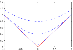
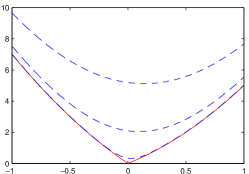
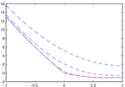
Figure 1: (a) The solid line represents the function |w|๐‘ค|w| and the dashed lines the bound โŸจ|w|โŸฉ๐’ฉโ€‹(wโ€‹ฮผ,ฯƒ2)subscriptdelimited-โŸจโŸฉ๐‘ค๐’ฉ๐‘ค๐œ‡superscript๐œŽ2\left\langle{|w|}\right\rangle_{{\cal{N}}\left({w\thinspace\vline\thinspace\mu,\sigma^{2}}\right)} plotted as a function of ฮผ๐œ‡\mu for three different values ฯƒโˆˆ{0.1,0.5,1}๐œŽ0.10.51\sigma\in\left\{{0.1,0.5,1}\right\} (from bottom to top in the figure). (b) The lasso objective function fโ€‹(w)๐‘“๐‘คf(w) plotted for A=2๐ด2A=2, ฮป=4๐œ†4\lambda=4, b=โˆ’1๐‘1b=-1, c=0๐‘0c=0. In this case the optimal setting for w๐‘คw based on the lasso objective is w=0๐‘ค0w=0. However, the optimal setting that minimizes the upper bound is slightly larger than zero. This means that the bound does not force the weights to exactly zero. (c) The lasso objective for A=2๐ด2A=2, ฮป=4๐œ†4\lambda=4, b=โˆ’7๐‘7b=-7, c=0๐‘0c=0. In this case the optimal setting for w๐‘คw for both the lasso objective and the variational bound are non-zero and numerically very close. This is to be expected since, as we move further away from the origin, the variational approximation more closely matches the objective, resulting in a closer match of their optima.

1.3 Bound optimization

VO provides a differentiable bound, whose optimum will still need to be found numerically. Since the bound if differentiable, any standard gradient-based method can be applied, such as Newton or Quasi-Newton methods. In the following sections, we discuss two example applications, the lasso and SVM objectives, both of which result in convex bound minimization problems. For the lasso problem we chose to use a simple diagonal approximation to Newtonโ€™s method to optimize the bound since this is simple to implement and often surprisingly effective. Naturally, more sophisticated procedures could be applied, though this is not the main focus of our interest here. For the SVM we chose L-BFGS, though again there are many alternatives that could be considered.

2 Sparse Least Squares Regression

The lasso is a well-known least squares regression estimator that encourages sparse solutions through a one-norm regularizer [3]. For D๐ทD-dimensional inputs xnsuperscript๐‘ฅ๐‘›x^{n}, outputs ynsuperscript๐‘ฆ๐‘›y^{n}, n=1,โ€ฆ,N๐‘›1โ€ฆ๐‘n=1,\ldots,N, and positive regularising constant ฮป๐œ†\lambda, the lasso objective is to minimize

fโ€‹(w)โ‰กโˆ‘n=1N(ynโˆ’wTโ€‹xn)2+ฮปโ€‹โˆ‘i=1D|wi|=c+wTโ€‹b+wTโ€‹Aโ€‹w+ฮปโ€‹โˆ‘i=1D|wi|๐‘“๐‘คsuperscriptsubscript๐‘›1๐‘superscriptsuperscript๐‘ฆ๐‘›superscript๐‘คTsuperscript๐‘ฅ๐‘›2๐œ†superscriptsubscript๐‘–1๐ทsubscript๐‘ค๐‘–๐‘superscript๐‘คT๐‘superscript๐‘คT๐ด๐‘ค๐œ†superscriptsubscript๐‘–1๐ทsubscript๐‘ค๐‘–f(w)\equiv\sum_{n=1}^{N}\left({y^{n}-w^{\textsf{T}}x^{n}}\right)^{2}+\lambda\sum_{i=1}^{D}|w_{i}|=c+w^{\textsf{T}}b+w^{\textsf{T}}Aw+\lambda\sum_{i=1}^{D}|w_{i}| (11)

with

cโ‰กโˆ‘n(yn)2,bโ‰กโˆ’2โ€‹โˆ‘nynโ€‹xn,andโ€‹Aโ‰กโˆ‘nxnโ€‹xnT.formulae-sequence๐‘subscript๐‘›superscriptsuperscript๐‘ฆ๐‘›2formulae-sequence๐‘2subscript๐‘›superscript๐‘ฆ๐‘›superscript๐‘ฅ๐‘›and๐ดsubscript๐‘›superscript๐‘ฅ๐‘›superscriptsuperscript๐‘ฅ๐‘›Tc\equiv\sum_{n}\left({y^{n}}\right)^{2},~{}~{}~{}b\equiv-2\sum_{n}y^{n}x^{n},~{}~{}~{}\text{and}~{}~{}~{}A\equiv\sum_{n}x^{n}{x^{n}}^{\textsf{T}}. (12)

The one-norm term โˆ‘i|wi|subscript๐‘–subscript๐‘ค๐‘–\sum_{i}|w_{i}| is non-differentiable at the origin and hence standard gradient based optimization algorithms cannot be directly applied. Section 1.2 shows that the variational bound conserves the convexity of an objective if a Gaussian (or more generally, expectation affine) distribution is used. Since the lasso objective is convex in w๐‘คw it is natural to consider a Gaussian variational distribution pโ€‹(w|ฮธ)=๐’ฉโ€‹(wโ€‹ฮผ,ฮฃ)๐‘conditional๐‘ค๐œƒ๐’ฉ๐‘ค๐œ‡ฮฃp(w|\theta)={\cal{N}}\left({w\thinspace\vline\thinspace\mu,\Sigma}\right) with mean ฮผ๐œ‡\mu and covariance ฮฃฮฃ\Sigma. This gives the upper bound fโˆ—โ‰คEโ€‹(ฮผ,C)superscript๐‘“๐ธ๐œ‡๐ถf^{*}\leq E(\mu,C), where

Eโ€‹(ฮผ,C)โ‰กโˆ‘nโŸจ(ynโˆ’wTโ€‹xn)2โŸฉ๐’ฉโ€‹(wโ€‹ฮผ,ฮฃ)+ฮปโ€‹โˆ‘iโŸจ|wi|โŸฉ๐’ฉโ€‹(wiโ€‹ฮผi,ฮฃiโ€‹i).๐ธ๐œ‡๐ถsubscript๐‘›subscriptdelimited-โŸจโŸฉsuperscriptsuperscript๐‘ฆ๐‘›superscript๐‘คTsuperscript๐‘ฅ๐‘›2๐’ฉ๐‘ค๐œ‡ฮฃ๐œ†subscript๐‘–subscriptdelimited-โŸจโŸฉsubscript๐‘ค๐‘–๐’ฉsubscript๐‘ค๐‘–subscript๐œ‡๐‘–subscriptฮฃ๐‘–๐‘–E(\mu,C)\equiv\sum_{n}\left\langle{\left({y^{n}-w^{\textsf{T}}{x}^{n}}\right)^{2}}\right\rangle_{{\cal{N}}\left({w\thinspace\vline\thinspace\mu,\Sigma}\right)}+\lambda\sum_{i}\left\langle{|w_{i}|}\right\rangle_{{\cal{N}}\left({w_{i}\thinspace\vline\thinspace\mu_{i},\Sigma_{ii}}\right)}. (13)

From Theorem 1, this is jointly convex in (ฮผ,C)๐œ‡๐ถ(\mu,C) where ฮฃ=Cโ€‹CTฮฃ๐ถsuperscript๐ถT\Sigma=CC^{\textsf{T}}, the Cholesky decomposition. It is straightforward to show that

โŸจ|w|โŸฉ๐’ฉโ€‹(wโ€‹ฮผ,ฯƒ2)=ฮผโ€‹(1โˆ’2โ€‹ฯ•โ€‹(โˆ’ฮผฯƒ))+2โ€‹ฯƒ2โ€‹ฯ€โ€‹eโˆ’ฮผ22โ€‹ฯƒ2subscriptdelimited-โŸจโŸฉ๐‘ค๐’ฉ๐‘ค๐œ‡superscript๐œŽ2๐œ‡12italic-ฯ•๐œ‡๐œŽ2๐œŽ2๐œ‹superscript๐‘’superscript๐œ‡22superscript๐œŽ2\left\langle{|{w}|}\right\rangle_{{\cal{N}}\left({w\thinspace\vline\thinspace\mu,\sigma^{2}}\right)}=\mu\bigg{(}1-2\phi\Big{(}-\frac{\mu}{\sigma}\Big{)}\bigg{)}+2\frac{\sigma}{\sqrt{2\pi}}e^{-\frac{\mu^{2}}{2\sigma^{2}}} (14)

where ฯ•โ€‹(x)=โˆซโˆ’โˆžxeโˆ’y2/2/2โ€‹ฯ€โ€‹๐‘‘yitalic-ฯ•๐‘ฅsuperscriptsubscript๐‘ฅsuperscript๐‘’superscript๐‘ฆ222๐œ‹differential-d๐‘ฆ\phi(x)=\int_{-\infty}^{x}e^{-y^{2}/2}/\sqrt{2\pi}dy is the cumulative density function of the standard normal distribution. More explicitly,

Eโ€‹(ฮผ,C)=c+ฮผTโ€‹b+ฮผTโ€‹Aโ€‹ฮผ+traceโ€‹(Aโ€‹ฮฃ)+ฮปโ€‹โˆ‘i(ฮผiโ€‹(1โˆ’2โ€‹ฯ•โ€‹(โˆ’ฮผiฯƒi))+2โ€‹ฯƒi2โ€‹ฯ€โ€‹eโˆ’ฮผi22โ€‹ฯƒi2)๐ธ๐œ‡๐ถ๐‘superscript๐œ‡T๐‘superscript๐œ‡T๐ด๐œ‡trace๐ดฮฃ๐œ†subscript๐‘–subscript๐œ‡๐‘–12italic-ฯ•subscript๐œ‡๐‘–subscript๐œŽ๐‘–2subscript๐œŽ๐‘–2๐œ‹superscript๐‘’superscriptsubscript๐œ‡๐‘–22superscriptsubscript๐œŽ๐‘–2E(\mu,C)=c+\mu^{\textsf{T}}b+\mu^{\textsf{T}}A\mu+{\rm trace}\left({A\Sigma}\right)+\lambda\sum_{i}\left({\mu_{i}\bigg{(}1-2\phi\Big{(}-\frac{\mu_{i}}{\sigma_{i}}\Big{)}\bigg{)}+2\frac{\sigma_{i}}{\sqrt{2\pi}}e^{-\frac{\mu_{i}^{2}}{2\sigma_{i}^{2}}}}\right) (15)

where ฯƒi2โ‰กฮฃiโ€‹isuperscriptsubscript๐œŽ๐‘–2subscriptฮฃ๐‘–๐‘–\sigma_{i}^{2}\equiv\Sigma_{ii}. The gradient and Hessian w.r.t ฮผ๐œ‡\mu are straightforward to compute using the results

โˆ‚โˆ‚ฮผโ€‹โŸจ|w|โŸฉ๐’ฉโ€‹(wโ€‹ฮผ,ฯƒ2)=1โˆ’2โ€‹ฯ•โ€‹(โˆ’ฮผฯƒ),โˆ‚2Eโˆ‚ฮผiโ€‹โˆ‚ฮผj=2โ€‹Aiโ€‹j+2โ€‹ฮป2โ€‹ฯ€โ€‹ฯƒi2โ€‹eโˆ’ฮผi22โ€‹ฯƒi2โ€‹ฮดiโ€‹j.formulae-sequence๐œ‡subscriptdelimited-โŸจโŸฉ๐‘ค๐’ฉ๐‘ค๐œ‡superscript๐œŽ212italic-ฯ•๐œ‡๐œŽsuperscript2๐ธsubscript๐œ‡๐‘–subscript๐œ‡๐‘—2subscript๐ด๐‘–๐‘—2๐œ†2๐œ‹subscriptsuperscript๐œŽ2๐‘–superscript๐‘’superscriptsubscript๐œ‡๐‘–22superscriptsubscript๐œŽ๐‘–2subscript๐›ฟ๐‘–๐‘—\frac{\partial}{\partial{\mu}}\left\langle{|{w}|}\right\rangle_{{\cal{N}}\left({w\thinspace\vline\thinspace\mu,\sigma^{2}}\right)}=1-2\phi\left({-\frac{\mu}{\sigma}}\right),\hskip 7.11317pt\frac{\partial^{2}E}{\partial\mu_{i}\partial\mu_{j}}=2\displaystyle A_{ij}+\frac{2\lambda}{\sqrt{2\pi\sigma^{2}_{i}}}e^{-\frac{\mu_{i}^{2}}{2\sigma_{i}^{2}}}\delta_{ij}. (16)

Since the bound is non-differentiable for ฮฃiโ€‹i=0subscriptฮฃ๐‘–๐‘–0\Sigma_{ii}=0, we use a fixed isotropic covariance ฮฃ=ฯƒ2โ€‹Iฮฃsuperscript๐œŽ2๐ผ\Sigma=\sigma^{2}I with ฯƒ>0๐œŽ0\sigma>0 and minimize the bound with respect to ฮผ๐œ‡\mu alone.

Refer to caption
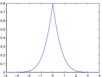
Figure 2: The function zโ€‹(1โˆ’2โ€‹ฯ•โ€‹(โˆ’z))+2ฯ€โ€‹eโˆ’z22โˆ’|z|๐‘ง12italic-ฯ•๐‘ง2๐œ‹superscript๐‘’superscript๐‘ง22๐‘งz\big{(}1-2\phi\left({-z}\right)\big{)}+\sqrt{\frac{2}{\pi}}e^{-\frac{z^{2}}{2}}-|{z}|.

2.1 Bounding the error

The difference between the bound and the function is given by (see Figure (1))

Eโ€‹(ฮผ)โˆ’fโ€‹(ฮผ)=traceโ€‹(Aโ€‹ฮฃ)+ฮปโ€‹โˆ‘iฯƒiโ€‹(ziโ€‹(1โˆ’2โ€‹ฯ•โ€‹(โˆ’zi))+2ฯ€โ€‹eโˆ’zi22โˆ’|zi|)๐ธ๐œ‡๐‘“๐œ‡trace๐ดฮฃ๐œ†subscript๐‘–subscript๐œŽ๐‘–subscript๐‘ง๐‘–12italic-ฯ•subscript๐‘ง๐‘–2๐œ‹superscript๐‘’superscriptsubscript๐‘ง๐‘–22subscript๐‘ง๐‘–E(\mu)-f(\mu)={\rm trace}\left({A\Sigma}\right)+\lambda\sum_{i}\sigma_{i}\left({z_{i}\left({1-2\phi\left({-z_{i}}\right)}\right)+\sqrt{\frac{2}{\pi}}e^{-\frac{z_{i}^{2}}{2}}-|{z_{i}}|}\right) (17)

where ziโ‰กฮผi/ฯƒisubscript๐‘ง๐‘–subscript๐œ‡๐‘–subscript๐œŽ๐‘–z_{i}\equiv\mu_{i}/\sigma_{i}. This splits into a set of independent terms, each of which has its maximum at zi=0subscript๐‘ง๐‘–0z_{i}=0, i.e. ฮผi=0subscript๐œ‡๐‘–0\mu_{i}=0, giving a maximal error of traceโ€‹(Aโ€‹ฮฃ)+2โ€‹ฮป2โ€‹ฯ€โ€‹โˆ‘iฯƒitrace๐ดฮฃ2๐œ†2๐œ‹subscript๐‘–subscript๐œŽ๐‘–{\rm trace}\left({A\Sigma}\right)+\frac{2\lambda}{\sqrt{2\pi}}\sum_{i}\sigma_{i}. Hence to guarantee to find a surrogate objective whose optimum value is within ฮ”fsubscriptฮ”๐‘“\Delta_{f} of the true lasso optimal value we must use, for ฮฃ=ฯƒ2โ€‹Iฮฃsuperscript๐œŽ2๐ผ\Sigma=\sigma^{2}I,

ฯƒโ‰ค1traceโ€‹(A)โ€‹((ฮป2โ€‹D22โ€‹ฯ€+ฮ”fโ€‹traceโ€‹(A))โˆ’ฮปโ€‹D2โ€‹ฯ€).๐œŽ1trace๐ดsuperscript๐œ†2superscript๐ท22๐œ‹subscriptฮ”๐‘“trace๐ด๐œ†๐ท2๐œ‹\sigma\leq\frac{1}{\sqrt{{\rm trace}\left({A}\right)}}\left({\sqrt{\left({\frac{\lambda^{2}D^{2}}{2\pi}+\Delta_{f}{\rm trace}\left({A}\right)}\right)}-\frac{\lambda D}{\sqrt{2\pi}}}\right). (18)

Hence, provided that ฯƒ๐œŽ\sigma is set small enough and assuming that the optimum of the bound is found accurately, we can guarantee to find the optimum value of the lasso objective to within some specified tolerance.

2.2 Lasso Experiments

We first generated a sparse D๐ทD-dimensional parameter vector with components uisubscript๐‘ข๐‘–u_{i} sampled according to

uiโˆผ{0with probability 0.5๐’ฉโ€‹(uiโ€‹โ€‰โ€‰5,1)with probability 0.25๐’ฉโ€‹(uiโˆ’5,1)with probability 0.25similar-tosubscript๐‘ข๐‘–cases0with probability 0.5๐’ฉsubscript๐‘ข๐‘–51with probability 0.25๐’ฉsubscript๐‘ข๐‘–51with probability 0.25u_{i}\sim\left\{\begin{array}[]{ll}0&\text{with probability 0.5}\\ {\cal{N}}\left({u_{i}\thinspace\vline\thinspace 5,1}\right)&\text{with probability 0.25}\\ {\cal{N}}\left({u_{i}\thinspace\vline\thinspace-5,1}\right)&\text{with probability 0.25}\\ \end{array}\right. (19)

We then created a set of N=10โ€‹D๐‘10๐ทN=10D training points in D๐ทD-dimensional space from the standard multivariate normal distribution ๐’ฉโ€‹(xโ€‹โ€‰โ€‰0,I)๐’ฉ๐‘ฅโ€‰โ€‰0๐ผ{\cal{N}}\left({x\thinspace\vline\thinspace 0,I}\right). The clean labels for these points were given by y0n=uTโ€‹xnsubscriptsuperscript๐‘ฆ๐‘›0superscript๐‘ขTsuperscript๐‘ฅ๐‘›y^{n}_{0}=u^{\textsf{T}}x^{n} and the final noisy labels by yn=y0n+ฯตnsuperscript๐‘ฆ๐‘›subscriptsuperscript๐‘ฆ๐‘›0superscriptitalic-ฯต๐‘›y^{n}=y^{n}_{0}+\epsilon^{n} where ฯตnsuperscriptitalic-ฯต๐‘›\epsilon^{n} is Gaussian random noise with mean zero and standard deviation 0.1โ€‹1Nโ€‹โˆ‘n=1N|y0n|0.11๐‘superscriptsubscript๐‘›1๐‘superscriptsubscript๐‘ฆ0๐‘›0.1\frac{1}{N}\sum_{n=1}^{N}|y_{0}^{n}|, chosen to obscure but not dominate the clean labels. We set ฮป=30โ€‹D๐œ†30๐ท\lambda=30D to give solutions with sparsity roughly the same as the initial parameter vector u๐‘ขu.

At each iteration we fixed ฮฃฮฃ\Sigma and updated ฮผ๐œ‡\mu using a diagonal approximation to the Newton method (to avoid the cost of inverting the full Hessian). For gradient Eiโ€ฒsubscriptsuperscript๐ธโ€ฒ๐‘–E^{\prime}_{i} and Hessian elements Eiโ€‹iโ€ฒโ€ฒsuperscriptsubscript๐ธ๐‘–๐‘–โ€ฒโ€ฒE_{ii}^{\prime\prime} the updates were

ฮผinโ€‹eโ€‹w=ฮผioโ€‹lโ€‹dโˆ’0.1โ€‹Eiโ€ฒEiโ€‹iโ€ฒโ€ฒ.subscriptsuperscript๐œ‡๐‘›๐‘’๐‘ค๐‘–superscriptsubscript๐œ‡๐‘–๐‘œ๐‘™๐‘‘0.1subscriptsuperscript๐ธโ€ฒ๐‘–subscriptsuperscript๐ธโ€ฒโ€ฒ๐‘–๐‘–\mu^{new}_{i}=\mu_{i}^{old}-0.1\frac{E^{\prime}_{i}}{E^{\prime\prime}_{ii}}. (20)

There is a trade-off between using a large ฯƒ๐œŽ\sigma, resulting in a bound whose optimum can be numerically obtained easily versus using a small ฯƒ๐œŽ\sigma for which the optimum of the bound is more difficult to find numerically, but for which the resulting bound optimum more closely matches the optimum of the true objective. Our experience is that in practice it is therefore best to start iterative procedures that optimize the bound with a relatively large ฯƒ๐œŽ\sigma, reducing this with each iteration. For this particular set of experiments we used an initial covariance matrix of 0.1 times the identity and reduced it by a factor of 0.9 at each iteration. The initial estimate for ฮผ๐œ‡\mu was a vector of zeros. We terminated when the mean absolute difference in the solution elements between iterations was less than 10โˆ’15superscript101510^{-15} of the mean absolute value of the elements of the current solution and took this terminal ฮผ๐œ‡\mu to be the estimate for argโกminwโกfโ€‹(w)subscript๐‘ค๐‘“๐‘ค\arg\min_{w}{f(w)}.

Small problems - D=50๐ท50D=50
Algorithm Solution time (SD) Relative Error (SD)
Variational optimization 0.1269 (0.0680) 3.791ร—10โˆ’14โ€‹(5.62ร—10โˆ’14)3.791superscript10145.62superscript10143.791\times 10^{-14}~{}(5.62\times 10^{-14})
Shooting 0.0142 (0.0037) 2.485ร—10โˆ’16โ€‹(2.21ร—10โˆ’16)2.485superscript10162.21superscript10162.485\times 10^{-16}~{}(2.21\times 10^{-16})
Iterated ridge regression 0.0268 (0.0208) 1.851ร—10โˆ’10โ€‹(6.27ร—10โˆ’10)1.851superscript10106.27superscript10101.851\times 10^{-10}~{}(6.27\times 10^{-10})
Smoothing (integral sigmoid) 0.1088 (0.0603) 4.421ร—10โˆ’15โ€‹(3.06ร—10โˆ’15)4.421superscript10153.06superscript10154.421\times 10^{-15}~{}(3.06\times 10^{-15})
Smoothing (x2+ฯตsuperscript๐‘ฅ2italic-ฯต\sqrt{x^{2}+\epsilon}) 0.0830 (0.0178) 4.916ร—10โˆ’15โ€‹(1.62ร—10โˆ’14)4.916superscript10151.62superscript10144.916\times 10^{-15}~{}(1.62\times 10^{-14})
Projection 0.0224 (0.0107) 2.672ร—10โˆ’16โ€‹(1.80ร—10โˆ’15)2.672superscript10161.80superscript10152.672\times 10^{-16}~{}(1.80\times 10^{-15})
Sub-gradients 0.0472 (0.0180) 9.176ร—10โˆ’10โ€‹(8.31ร—10โˆ’09)9.176superscript10108.31superscript10099.176\times 10^{-10}~{}(8.31\times 10^{-09})
Larger problems - D=200๐ท200D=200
Algorithm Solution time (SD) Relative Error (SD)
Variational optimization 0.1308 (0.0405) 1.923ร—10โˆ’15โ€‹(6.01ร—10โˆ’16)1.923superscript10156.01superscript10161.923\times 10^{-15}~{}(6.01\times 10^{-16})
Shooting 0.0676 (0.0209) 2.656ร—10โˆ’16โ€‹(3.17ร—10โˆ’16)2.656superscript10163.17superscript10162.656\times 10^{-16}~{}(3.17\times 10^{-16})
Iterated ridge regression 0.1645 (0.0844) 4.004ร—10โˆ’14โ€‹(1.19ร—10โˆ’13)4.004superscript10141.19superscript10134.004\times 10^{-14}~{}(1.19\times 10^{-13})
Smoothing (integral sigmoid) 1.2305 (0.3381) 2.638ร—10โˆ’15โ€‹(9.19ร—10โˆ’16)2.638superscript10159.19superscript10162.638\times 10^{-15}~{}(9.19\times 10^{-16})
Smoothing (x2+ฯตsuperscript๐‘ฅ2italic-ฯต\sqrt{x^{2}+\epsilon}) 1.1385 (0.3673) 1.471ร—10โˆ’15โ€‹(1.86ร—10โˆ’15)1.471superscript10151.86superscript10151.471\times 10^{-15}~{}(1.86\times 10^{-15})
Projection 0.3121 (0.0726) 5.325ร—10โˆ’16โ€‹(2.85ร—10โˆ’16)5.325superscript10162.85superscript10165.325\times 10^{-16}~{}(2.85\times 10^{-16})
Sub-gradients 1.3478 (0.3273) 6.038ร—10โˆ’11โ€‹(9.42ร—10โˆ’10)6.038superscript10119.42superscript10106.038\times 10^{-11}~{}(9.42\times 10^{-10})
Table 1: Performance and time taken (in seconds) for algorithms solving lasso problems of two different sizes. All algorithms were implemented in MATLAB and run on a 2.27GHz 4GB machine. The averages and the standard deviations result from 500 experiments.

We tested our method against a number of standard lasso solvers in Mark Schmidtโ€™s minFunc MATLAB package333www.di.ens.fr/โˆผsimilar-to\simmschmidt/Software/minFunc.html to gain an indication of its performance relative to established approaches. Since the true optima are not known, we measured the success of the algorithms relative to the best solution fbestsubscript๐‘“bestf_{\text{best}}, found by any of the algorithms on each problem instance. In Table 1 we give the mean and standard deviation of relative errors (fโˆ’fbest)/(fbest)๐‘“subscript๐‘“bestsubscript๐‘“best(f-f_{\text{best}})/(f_{\text{best}}). The results indicate that VO is capable of approximating the global optimum in moderate time and that it scales well with problem size. In particular, VO provides solutions of similar quality to other smoothed methods in [4] (the first based on approximating the L1subscript๐ฟ1L_{1} norm using an integral of two sigmoid functions and the second using x2+ฯตsuperscript๐‘ฅ2italic-ฯต\sqrt{x^{2}+\epsilon} where ฯตitalic-ฯต\epsilon is some positive constant)444The improvement of VO over other smoothing approaches is most likely accounted for by implementation differences and our reduction of ฯƒ๐œŽ\sigma at each iteration..

2.3 Fused Lasso Sparse Regression

From table(1), the standard lasso problem is most effectively solved by the shooting algorithm [5]. Shooting corresponds to solving each component whilst keeping the others fixed, and subsequently cycling through components to convergence. This is particularly effective in the standard lasso problem since the corresponding one-dimensional optima for each component can be found in closed form; also the objective only weakly couples the components of the vector w๐‘คw. In contrast, the fused lasso problem induces additional sparsity between adjacent elements using the objective:

fโ€‹(w)=c+wTโ€‹b+wTโ€‹Aโ€‹w+ฮป1โ€‹โˆ‘i=1D|wi|+ฮป2โ€‹โˆ‘i=2D|wiโˆ’wiโˆ’1|๐‘“๐‘ค๐‘superscript๐‘คT๐‘superscript๐‘คT๐ด๐‘คsubscript๐œ†1superscriptsubscript๐‘–1๐ทsubscript๐‘ค๐‘–subscript๐œ†2superscriptsubscript๐‘–2๐ทsubscript๐‘ค๐‘–subscript๐‘ค๐‘–1f(w)=c+w^{\textsf{T}}b+w^{\textsf{T}}Aw+\lambda_{1}\sum_{i=1}^{D}|w_{i}|+\lambda_{2}\sum_{i=2}^{D}|w_{i}-w_{i-1}| (21)

The additional term also introduces strong dependencies between adjacent components and componentwise (โ€™shootingโ€™) methods struggle to converge [6]. In applying VO, with ฮฃ=ฯƒ2โ€‹Iฮฃsuperscript๐œŽ2๐ผ\Sigma=\sigma^{2}I, the additional terms โŸจ|wiโˆ’wiโˆ’1|โŸฉ๐’ฉโ€‹(wโ€‹ฮผ,ฯƒ2โ€‹I)subscriptdelimited-โŸจโŸฉsubscript๐‘ค๐‘–subscript๐‘ค๐‘–1๐’ฉ๐‘ค๐œ‡superscript๐œŽ2๐ผ\left\langle{|{w_{i}-w_{i-1}}|}\right\rangle_{{\cal{N}}\left({w\thinspace\vline\thinspace\mu,\sigma^{2}I}\right)} in the bound are given by:

(ฮผiโˆ’ฮผiโˆ’1)โ€‹(1โˆ’2โ€‹ฯ•โ€‹(ฮผiโˆ’1โˆ’ฮผi2โ€‹ฯƒ))+2โ€‹ฯƒฯ€โ€‹eโˆ’(ฮผiโˆ’ฮผiโˆ’1)24โ€‹ฯƒ2subscript๐œ‡๐‘–subscript๐œ‡๐‘–112italic-ฯ•subscript๐œ‡๐‘–1subscript๐œ‡๐‘–2๐œŽ2๐œŽ๐œ‹superscript๐‘’superscriptsubscript๐œ‡๐‘–subscript๐œ‡๐‘–124superscript๐œŽ2\displaystyle(\mu_{i}-\mu_{i-1})\bigg{(}1-2\phi\Big{(}\frac{\mu_{i-1}-\mu_{i}}{\sqrt{2}\sigma}\Big{)}\bigg{)}+\frac{2\sigma}{\sqrt{\pi}}e^{\frac{-(\mu_{i}-\mu_{i-1})^{2}}{4\sigma^{2}}} (22)

As for the standard lasso case, we can readily obtain the gradient and Hessian of the objective.

2.4 Fused Lasso Experiments

We set the D๐ทD-dimensional parameter vector so that there would be some real underlying sparsity in the differences between elements of the optimum w๐‘คw. The first element in the parameter vector u1subscript๐‘ข1u_{1} was generated as in the previous problem, then all subsequent elements were generated by:

ui>1โˆผ{uiโˆ’1with probability 0.50with probability 0.25๐’ฉโ€‹(uiโ€‹โ€‰โ€‰5,1)with probability 0.125๐’ฉโ€‹(uiโˆ’5,1)with probability 0.125similar-tosubscript๐‘ข๐‘–1casessubscript๐‘ข๐‘–1with probability 0.50with probability 0.25๐’ฉsubscript๐‘ข๐‘–51with probability 0.125๐’ฉsubscript๐‘ข๐‘–51with probability 0.125u_{i>1}\sim\left\{\begin{array}[]{ll}u_{i-1}&\text{with probability 0.5}\\ 0&\text{with probability 0.25}\\ {\cal{N}}\left({u_{i}\thinspace\vline\thinspace 5,1}\right)&\text{with probability 0.125}\\ {\cal{N}}\left({u_{i}\thinspace\vline\thinspace-5,1}\right)&\text{with probability 0.125}\\ \end{array}\right. (23)

We again created a set of N=10โ€‹D๐‘10๐ทN=10D training points in D๐ทD-dimensional space from the standard multivariate normal distribution. The clean labels for these points were then given by y0n=uTโ€‹xnsubscriptsuperscript๐‘ฆ๐‘›0superscript๐‘ขTsuperscript๐‘ฅ๐‘›y^{n}_{0}=u^{\textsf{T}}x^{n} and the final noisy labels by yn=y0n+ฯตnsuperscript๐‘ฆ๐‘›subscriptsuperscript๐‘ฆ๐‘›0superscriptitalic-ฯต๐‘›y^{n}=y^{n}_{0}+\epsilon^{n} where ฯตnsuperscriptitalic-ฯต๐‘›\epsilon^{n} is random noise with mean zero and standard deviation 0.1โ€‹1Nโ€‹โˆ‘n=1N|y0n|0.11๐‘superscriptsubscript๐‘›1๐‘superscriptsubscript๐‘ฆ0๐‘›0.1\frac{1}{N}\sum_{n=1}^{N}|y_{0}^{n}|.

We ran a D=500๐ท500D=500 experiment 1000 times with ฮป1=500subscript๐œ†1500\lambda_{1}=500 and ฮป2=200subscript๐œ†2200\lambda_{2}=200. These values were chosen to give rise to a problem in which the loss function had a significant impact but did not enforce more sparsity than was typically present in the original parameter vector u๐‘ขu. The initial standard deviation was 0.1, and we shrunk it by 0.9 at each iteration. For comparison we used the SLEP package [7], which has very competitive performance compared to other state-of-the-art solvers. The SLEP package is based on a version of Nesterovโ€™s method [8], a two step gradient method with backtracking line search. Using a shrinking variance and a convergence tolerance of 10โˆ’6superscript10610^{-6}, the mean relative error in terms of function value of VO compared to SLEP was 1.59ร—10โˆ’41.59superscript1041.59\times 10^{-4}. The mean of the relative distances L2โ€‹(xโˆ’y)/L2โ€‹(y)subscript๐ฟ2๐‘ฅ๐‘ฆsubscript๐ฟ2๐‘ฆL_{2}(x-y)/L_{2}(y) between each VO solution x๐‘ฅx and SLEP solution y๐‘ฆy was 0.0135. The mean CPU time for VO was 0.0947s and for the SLEP algorithm 0.0724s555SLEP is implemented in C, so the comparison of speed with our MATLAB implementation is not definitive.. Compared to other approaches, our method is very simple to implement and has good performance compared to the state of the art.

3 Soft Margin Support Vector Machines

The support vector machine (SVM) is a method for finding the optimal separating hyperplane of set of N๐‘N data points xnsuperscript๐‘ฅ๐‘›x^{n} with labels yn=ยฑ1superscript๐‘ฆ๐‘›plus-or-minus1y^{n}=\pm 1. This separating hyperplane may be in the space of the data points, or in a higher dimensional feature space if linear separation is not possible. In this second case, the data points are mapped to the feature space with a function ฯ†โ€‹(xn)๐œ‘superscript๐‘ฅ๐‘›\varphi(x^{n}). When the data are not separable the soft margin support vector machine is used. This adds slack variables ฮพnsuperscript๐œ‰๐‘›\xi^{n} which allow misclassified data points at a cost controlled by a variable C๐ถC. The complete soft margin support vector machine has primal form:

minw,b,ฮพโกw๐–ณโ€‹w+Cโ€‹โˆ‘n=1Nฮพnsubscript๐‘ค๐‘๐œ‰superscript๐‘ค๐–ณ๐‘ค๐ถsuperscriptsubscript๐‘›1๐‘superscript๐œ‰๐‘›\displaystyle\displaystyle\min_{w,b,\xi}w^{\mathsf{T}}w+C\displaystyle\sum_{n=1}^{N}\xi^{n} (24)
subject toโ€‹ynโ€‹(w๐–ณโ€‹ฯ†โ€‹(xn)+b)โ‰ฅ1โˆ’ฮพnโ€‹Cโ€‹andโ€‹ฮพnโ‰ฅ0.subject tosuperscript๐‘ฆ๐‘›superscript๐‘ค๐–ณ๐œ‘superscript๐‘ฅ๐‘›๐‘1superscript๐œ‰๐‘›๐ถandsuperscript๐œ‰๐‘›0\displaystyle\text{subject to}~{}~{}y^{n}(w^{\mathsf{T}}\varphi(x^{n})+b)\geq 1-\xi^{n}C~{}~{}\text{and}~{}~{}\xi^{n}\geq 0. (25)

This is classically solved by the method of Lagrange multipliers [9]. This yields a convex, constrained quadratic program referred to as the dual problem. The dual form is often preferred because it provides a convenient way to deal with the constraints, and because kernel methods can be easily applied.

As an alternative, the primal problem can be re-expressed as a convex, unconstrained problem (see, for example, [10]). To remove the constraints from the primal problem, note that the objective is minimized when the slack variables ฮพnsuperscript๐œ‰๐‘›\xi^{n} are as small as possible without violating the constraints. This is achieved by setting ฮพn=maxโก{ynโ€‹(w๐–ณโ€‹ฯ†โ€‹(xn)+b)โˆ’1,0}superscript๐œ‰๐‘›superscript๐‘ฆ๐‘›superscript๐‘ค๐–ณ๐œ‘superscript๐‘ฅ๐‘›๐‘10\xi^{n}=\max\{y^{n}(w^{\mathsf{T}}\varphi(x^{n})+b)-1,0\}, yielding the objective to be minimized:

fโ€‹(w,b)=w๐–ณโ€‹w+Cโ€‹โˆ‘n=1Nmaxโก{1โˆ’ynโ€‹(w๐–ณโ€‹ฯ†โ€‹(xn)+b),0}.๐‘“๐‘ค๐‘superscript๐‘ค๐–ณ๐‘ค๐ถsuperscriptsubscript๐‘›1๐‘1superscript๐‘ฆ๐‘›superscript๐‘ค๐–ณ๐œ‘superscript๐‘ฅ๐‘›๐‘0f(w,b)=w^{\mathsf{T}}w+C\displaystyle\sum_{n=1}^{N}\max\{1-y^{n}(w^{\mathsf{T}}\varphi(x^{n})+b),0\}. (26)

These slack variable terms are hinge loss penalties on misclassified data points. The hinge loss is convex in w๐‘คw and b๐‘b, thus the whole objective (a sum of hinge losses plus a convex quadratic term) is convex. It has discontinuities across each of the hyperplanes w๐–ณโ€‹ฯ†โ€‹(xn)+b=ynsuperscript๐‘ค๐–ณ๐œ‘superscript๐‘ฅ๐‘›๐‘superscript๐‘ฆ๐‘›w^{\mathsf{T}}\varphi(x^{n})+b=y^{n}. To allow feature mapping we must solve the primal problem in a reproducing kernel Hilbert space without using Lagrange multipliers. Without loss of generality, we may assume that the solution w๐‘คw can be expressed as

w=โˆ‘n=1Nฮฒnโ€‹ynโ€‹ฯ†โ€‹(xn)๐‘คsuperscriptsubscript๐‘›1๐‘superscript๐›ฝ๐‘›superscript๐‘ฆ๐‘›๐œ‘superscript๐‘ฅ๐‘›w=\sum_{n=1}^{N}\beta^{n}y^{n}\varphi(x^{n}) (27)

which gives rise to the kernelized objective function:

fโ€‹(ฮฒ,b)=ฮฒTโ€‹Kโ€‹ฮฒ+Cโ€‹โˆ‘n=1Nmaxโก{1โˆ’โˆ‘m=1NKnโ€‹mโ€‹ฮฒmโˆ’bโ€‹yn,0}๐‘“๐›ฝ๐‘superscript๐›ฝT๐พ๐›ฝ๐ถsuperscriptsubscript๐‘›1๐‘1superscriptsubscript๐‘š1๐‘subscript๐พ๐‘›๐‘šsuperscript๐›ฝ๐‘š๐‘superscript๐‘ฆ๐‘›0f(\beta,b)=\beta^{\textsf{T}}K\beta+C\sum_{n=1}^{N}\max\{1-\sum_{m=1}^{N}K_{nm}\beta^{m}-by^{n},0\} (28)

where the kernel matrix is given by Knโ€‹m=ynโ€‹ymโ€‹ฯ†โ€‹(xn)๐–ณโ€‹ฯ†โ€‹(xm)subscript๐พ๐‘›๐‘šsuperscript๐‘ฆ๐‘›superscript๐‘ฆ๐‘š๐œ‘superscriptsuperscript๐‘ฅ๐‘›๐–ณ๐œ‘superscript๐‘ฅ๐‘šK_{nm}=y^{n}y^{m}{\varphi(x^{n})}^{\mathsf{T}}\varphi(x^{m}). This kernelized problem is convex; however it is discontinuous and therefore not directly amenable to gradient descent methods.

The variational bound is the expectation of f๐‘“f with respect to distributions over ฮฒ๐›ฝ\beta and b๐‘b. We choose again Gaussian distributions over the parameters: ฮฒ๐›ฝ\beta distributed with mean ฮผฮฒsubscript๐œ‡๐›ฝ\mu_{\beta} and covariance ฯƒ2โ€‹Isuperscript๐œŽ2๐ผ\sigma^{2}I and b๐‘b independently with mean ฮผbsubscript๐œ‡๐‘\mu_{b} and variance ฯƒ2superscript๐œŽ2\sigma^{2}. This gives the bound fโˆ—โ‰คEsuperscript๐‘“๐ธf^{*}\leq E with

Eโ‰กโŸจfโ€‹(ฮฒ,b)โŸฉpโ€‹(ฮฒ,b|ฮผฮฒ,ฮผb)=ฮผฮฒTโ€‹Kโ€‹ฮผฮฒ+traceโ€‹(ฯƒ2โ€‹K)+Cโ€‹โˆ‘n=1N(ฮฝnโ€‹ฯ•โ€‹(ฮฝnฯ‚n)+ฯ‚n2โ€‹ฯ€โ€‹eโˆ’12โ€‹(ฮฝnฯ‚n)2)๐ธsubscriptdelimited-โŸจโŸฉ๐‘“๐›ฝ๐‘๐‘๐›ฝconditional๐‘subscript๐œ‡๐›ฝsubscript๐œ‡๐‘superscriptsubscript๐œ‡๐›ฝT๐พsubscript๐œ‡๐›ฝtracesuperscript๐œŽ2๐พ๐ถsuperscriptsubscript๐‘›1๐‘superscript๐œˆ๐‘›italic-ฯ•superscript๐œˆ๐‘›superscript๐œ๐‘›superscript๐œ๐‘›2๐œ‹superscript๐‘’12superscriptsuperscript๐œˆ๐‘›superscript๐œ๐‘›2E\equiv\langle f(\beta,b)\rangle_{p(\beta,b|\mu_{\beta},\mu_{b})}=\mu_{\beta}^{\textsf{T}}K\mu_{\beta}+\text{trace}(\sigma^{2}K)+C\sum_{n=1}^{N}\left(\nu^{n}\phi\left(\frac{\nu^{n}}{\varsigma^{n}}\right)+\frac{\varsigma^{n}}{\sqrt{2\pi}}e^{-\frac{1}{2}\left(\frac{\nu^{n}}{\varsigma^{n}}\right)^{2}}\right) (29)

where

ฮฝn=1โˆ’โˆ‘m=1NKnโ€‹mโ€‹ฮผฮฒm+ฮผbโ€‹yn,ฯ‚n=ฯƒ2+โˆ‘m=1NKnโ€‹m2โ€‹ฯƒ2.formulae-sequencesuperscript๐œˆ๐‘›1superscriptsubscript๐‘š1๐‘subscript๐พ๐‘›๐‘šsuperscriptsubscript๐œ‡๐›ฝ๐‘šsubscript๐œ‡๐‘superscript๐‘ฆ๐‘›superscript๐œ๐‘›superscript๐œŽ2superscriptsubscript๐‘š1๐‘superscriptsubscript๐พ๐‘›๐‘š2superscript๐œŽ2\nu^{n}=1-\sum_{m=1}^{N}K_{nm}\mu_{\beta}^{m}+\mu_{b}y^{n},\hskip 28.45274pt\varsigma^{n}=\sqrt{\sigma^{2}+\sum_{m=1}^{N}K_{nm}^{2}\sigma^{2}}. (30)

The gradients used in optimizing the variational objective can then also be calculated explicitly:

โˆ‚Eโˆ‚ฮผฮฒn๐ธsuperscriptsubscript๐œ‡๐›ฝ๐‘›\displaystyle\frac{\partial E}{\partial\mu_{\beta}^{n}} =โˆ‘m=1N2โ€‹Knโ€‹mโ€‹ฮผฮฒmโˆ’Cโ€‹โˆ‘m=1NKnโ€‹mฯ‚mโ€‹ฯ•โ€‹(ฮฝmฯ‚m)absentsuperscriptsubscript๐‘š1๐‘2subscript๐พ๐‘›๐‘šsuperscriptsubscript๐œ‡๐›ฝ๐‘š๐ถsuperscriptsubscript๐‘š1๐‘subscript๐พ๐‘›๐‘šsuperscript๐œ๐‘šitalic-ฯ•superscript๐œˆ๐‘šsuperscript๐œ๐‘š\displaystyle=\sum_{m=1}^{N}2K_{nm}\mu_{\beta}^{m}-C\sum_{m=1}^{N}\frac{K_{nm}}{\varsigma^{m}}\phi\left(\frac{\nu^{m}}{\varsigma^{m}}\right) (31)
โˆ‚Eโˆ‚b๐ธ๐‘\displaystyle\frac{\partial E}{\partial b} =โˆ’Cโ€‹โˆ‘m=1Nymฯ‚mโ€‹ฯ•โ€‹(ฮฝmฯ‚m)absent๐ถsuperscriptsubscript๐‘š1๐‘superscript๐‘ฆ๐‘šsuperscript๐œ๐‘šitalic-ฯ•superscript๐œˆ๐‘šsuperscript๐œ๐‘š\displaystyle=-C\sum_{m=1}^{N}\frac{y^{m}}{\varsigma^{m}}\phi\left(\frac{\nu^{m}}{\varsigma^{m}}\right) (32)

We can also bound the difference between the variational and original objectives, just as we did in the lasso case. The difference between the bound and the function is given by

Eโ€‹(ฮผฮฒ,ฮผb)โˆ’fโ€‹(ฮผฮฒ,ฮผb)=traceโ€‹(ฯƒ2โ€‹K)+Cโ€‹โˆ‘n=1N(ฮฝnโ€‹ฯ•โ€‹(ฮฝnฯ‚n)+ฯ‚n2โ€‹ฯ€โ€‹eโˆ’12โ€‹(ฮฝnฯ‚n)2โˆ’maxโก{ฮฝn,0})๐ธsubscript๐œ‡๐›ฝsubscript๐œ‡๐‘๐‘“subscript๐œ‡๐›ฝsubscript๐œ‡๐‘tracesuperscript๐œŽ2๐พ๐ถsuperscriptsubscript๐‘›1๐‘superscript๐œˆ๐‘›italic-ฯ•superscript๐œˆ๐‘›superscript๐œ๐‘›superscript๐œ๐‘›2๐œ‹superscript๐‘’12superscriptsuperscript๐œˆ๐‘›superscript๐œ๐‘›2superscript๐œˆ๐‘›0E(\mu_{\beta},\mu_{b})-f(\mu_{\beta},\mu_{b})={\rm trace}\left({\sigma^{2}K}\right)+C\sum_{n=1}^{N}\left(\nu^{n}\phi\left(\frac{\nu^{n}}{\varsigma^{n}}\right)+\frac{\varsigma^{n}}{\sqrt{2\pi}}e^{-\frac{1}{2}\left(\frac{\nu^{n}}{\varsigma^{n}}\right)^{2}}-\max\{\nu^{n},0\}\right) (33)

The terms of the sum are each maximized at ฮฝn=0superscript๐œˆ๐‘›0\nu^{n}=0. ฮฝnsuperscript๐œˆ๐‘›\nu^{n} are not independent, so these conditions are unlikely to occur simultaneously, but we can bound the difference by

Eโ€‹(ฮผฮฒ,ฮผb)โˆ’fโ€‹(ฮผฮฒ,ฮผb)โ‰คtraceโ€‹(ฯƒ2โ€‹K)+Cโ€‹โˆ‘n=1Nฯ‚n2โ€‹ฯ€.๐ธsubscript๐œ‡๐›ฝsubscript๐œ‡๐‘๐‘“subscript๐œ‡๐›ฝsubscript๐œ‡๐‘tracesuperscript๐œŽ2๐พ๐ถsuperscriptsubscript๐‘›1๐‘superscript๐œ๐‘›2๐œ‹E(\mu_{\beta},\mu_{b})-f(\mu_{\beta},\mu_{b})\leq{\rm trace}\left({\sigma^{2}K}\right)+C\sum_{n=1}^{N}\frac{\varsigma^{n}}{\sqrt{2\pi}}. (34)

To guarantee to find a surrogate SVM objective whose optimum is within a specified function tolerance ฮ”fsubscriptฮ”๐‘“\Delta_{f}, one must thus satisfy

ฯƒโ‰ค1traceโ€‹(K)โ€‹((C2โ€‹M28โ€‹ฯ€+ฮ”fโ€‹traceโ€‹(K))โˆ’Cโ€‹M8โ€‹ฯ€)๐œŽ1trace๐พsuperscript๐ถ2superscript๐‘€28๐œ‹subscriptฮ”๐‘“trace๐พ๐ถ๐‘€8๐œ‹\sigma\leq\frac{1}{\sqrt{{\rm trace}\left({K}\right)}}\left({\sqrt{\left({\frac{C^{2}M^{2}}{8\pi}+\Delta_{f}{\rm trace}\left({K}\right)}\right)}-\frac{CM}{\sqrt{8\pi}}}\right) (35)

where

M=โˆ‘n=1N1+โˆ‘m=1NKnโ€‹m2.๐‘€superscriptsubscript๐‘›1๐‘1superscriptsubscript๐‘š1๐‘superscriptsubscript๐พ๐‘›๐‘š2M=\displaystyle\sum_{n=1}^{N}\sqrt{1+\sum_{m=1}^{N}{K_{nm}^{2}}}. (36)
Refer to caption
Refer to caption
Refer to caption
Refer to caption
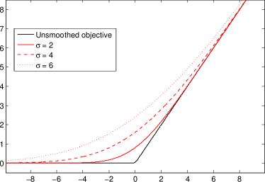
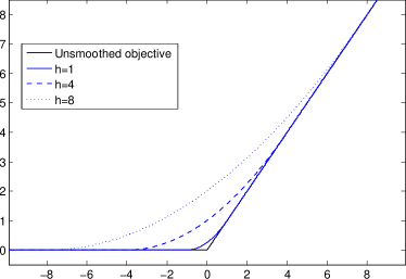
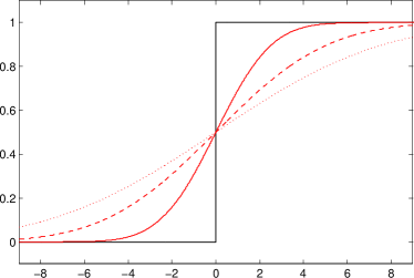
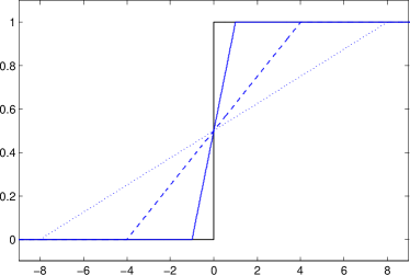
Figure 3: (a) hinge loss and VO smoothed hinge loss; (b) Huber loss; (c) smoothed hinge loss gradient; (d) Huber loss gradient.

3.1 Chapelleโ€™s smoothing method

Chapelle [10] formulates the problem as in Equation(28), though allowing for any form of loss function L๐ฟL rather than just the hinge loss.

EChapelleโ€‹(ฮฒ,b)=ฮฒTโ€‹Kโ€‹ฮฒ+Cโ€‹โˆ‘n=1NLโ€‹(1โˆ’โˆ‘m=1Nฮฒmโ€‹Knโ€‹mโˆ’bโ€‹yn)subscript๐ธChapelle๐›ฝ๐‘superscript๐›ฝT๐พ๐›ฝ๐ถsuperscriptsubscript๐‘›1๐‘๐ฟ1superscriptsubscript๐‘š1๐‘superscript๐›ฝ๐‘šsubscript๐พ๐‘›๐‘š๐‘superscript๐‘ฆ๐‘›E_{\text{Chapelle}}(\beta,b)=\beta^{\textsf{T}}K\beta+C\sum_{n=1}^{N}L(1-\sum_{m=1}^{N}\beta^{m}K_{nm}-by^{n}) (37)

He then derives Newton methods with quadratic loss and, more relevant to our problem, the Huber loss:

LHuberโ€‹(ฮพ)={(1+hโ€‹ฮพ)24โ€‹hifโ€‹|ฮพ|<hmaxโก{ฮพ,0}otherwisesubscript๐ฟHuber๐œ‰casessuperscript1โ„Ž๐œ‰24โ„Žif๐œ‰โ„Ž๐œ‰0otherwiseL_{\text{Huber}}(\xi)=\left\{\begin{array}[]{ll}\frac{(1+h\xi)^{2}}{4h}&\text{if}~{}~{}|\xi|<h\\ \max\{\xi,0\}&\text{otherwise}\end{array}\right. (38)

The form of the Huber loss can be seen in Figure (3). It is an upper bound on the hinge loss, fโˆ—โ‰คEChapellesuperscript๐‘“subscript๐ธChapellef^{*}\leq E_{\text{Chapelle}}, and becomes tighter for smaller hโ„Žh. This bound can be used in the same way as the variational bound, giving a smoothed approximation to the SVM objective. As with VO, the objective is a sum of convex terms and is thus itself convex. The Hessian of EChapellesubscript๐ธChapelleE_{\text{Chapelle}} is given by

H=(โˆ‚2EChapelleโˆ‚b2โˆ‚2EChapelleโˆ‚bโ€‹โˆ‚ฮฒโˆ‚2EChapelleโˆ‚ฮฒโ€‹โˆ‚bโˆ‚2EChapelleโˆ‚ฮฒ2)=2โ€‹Cโ€‹(1๐–ณโ€‹Iqโ€‹11๐–ณโ€‹Iqโ€‹KKโ€‹Iqโ€‹11Cโ€‹K+Kโ€‹Iqโ€‹K)๐ปsuperscript2subscript๐ธChapellesuperscript๐‘2superscript2subscript๐ธChapelle๐‘๐›ฝsuperscript2subscript๐ธChapelle๐›ฝ๐‘superscript2subscript๐ธChapellesuperscript๐›ฝ22๐ถsuperscript1๐–ณsuperscript๐ผ๐‘ž1superscript1๐–ณsuperscript๐ผ๐‘ž๐พ๐พsuperscript๐ผ๐‘ž11๐ถ๐พ๐พsuperscript๐ผ๐‘ž๐พH=\left(\begin{array}[]{ll}\frac{\partial^{2}E_{\text{Chapelle}}}{\partial b^{2}}&\frac{\partial^{2}E_{\text{Chapelle}}}{\partial b\partial\beta}\\ \frac{\partial^{2}E_{\text{Chapelle}}}{\partial\beta\partial b}&\frac{\partial^{2}E_{\text{Chapelle}}}{\partial\beta^{2}}\end{array}\right)=2C\left(\begin{array}[]{ll}1^{\mathsf{T}}I^{q}1&1^{\mathsf{T}}I^{q}K\\ KI^{q}1&\frac{1}{C}K+KI^{q}K\end{array}\right) (39)

where 111 is a vector of ones of dimension N๐‘N and Iqsuperscript๐ผ๐‘žI^{q} is a diagonal matrix indicating whether a given data point is in the quadratic portion of the loss function:

Inโ€‹nq={1ifโ€‹|1โˆ’โˆ‘m=1Nฮฒmโ€‹Knโ€‹m+bโ€‹yn|<h0otherwisesubscriptsuperscript๐ผ๐‘ž๐‘›๐‘›cases1if1superscriptsubscript๐‘š1๐‘superscript๐›ฝ๐‘šsubscript๐พ๐‘›๐‘š๐‘superscript๐‘ฆ๐‘›โ„Ž0otherwiseI^{q}_{nn}=\left\{\begin{array}[]{ll}1&\text{if}~{}~{}|1-\sum_{m=1}^{N}\beta^{m}K_{nm}+by^{n}|<h\\ 0&\text{otherwise}\end{array}\right. (40)

Given that we wish to optimize the hinge loss, we must choose hโ„Žh to be small. The quadratic region in the Huber loss is then small and as a consequence it is likely that for some trial solutions no training points will lie in this quadratic portion. This results in a value of zero for all Hessian elements corresponding to the offset (all blocks in the black matrix in Equation(39) except the bottom right). The Hessian is therefore non-invertible and Chapelleโ€™s Newton update cannot be evaluated. If instead the L-BFGS method is used [11] it can easily be shown that the approximate Hessian is always positive definite and thus Newton-like performance can be achieved without risking invalid updates. This also means the cubic cost of inversion in the full Newton method is avoided.

3.2 SVM Experiments

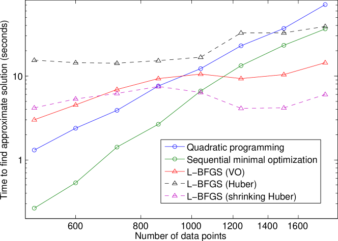
Synthetic problems were constructed by generating a random separation vector of length 3.5 and dimension 100. The length of this vector was chosen to give a problem which could be mostly, but not completely, separated using a linear kernel. The positively labelled points were then distributed with a standard multivariate normal about this separation vector and the negatively labelled points with the same distribution about the origin. The objective we used had a cost coefficient C=10๐ถ10C=10. We define approximate convergence as finding a function value with relative error (fโˆ—โˆ’ffsuperscript๐‘“๐‘“๐‘“\frac{f^{*}-f}{f}) of less than 0.1% compared to the function value fโˆ—superscript๐‘“f^{*} of the MATLAB quadratic program on the dual when run until completion. For each of 50 training sets for each training set size, each method was given the same initial solution (a vector generated from a standard normal distribution) and run until approximate convergence.

We compared VO to a modification of Chapelleโ€™s method (with and without shrinking the Huber parameter), sequential minimal optimization (SMO) and quadratic programming on the dual problem. We applied Chapelleโ€™s method by optimizing a Huber loss smoothed function using the L-BFGS implementation in the minFunc package. To ensure comparability we treated VO in the same way, with the additional consideration of variance reduction at each iteration. We shrank the variance by a factor of 10 every 250 iterations, from an initial value of 0.001. The Huber loss function was similarly shrunk by a factor of 10 every 250 iterations, but from an initial value of 10. SMO [12] solves the dual by analytically solving a sub-problem in two components and iterating until convergence. We used the implementation in the BRML toolbox [13], which is based on the working set selection proposed by [14]. The dual was solved using the MATLAB built in function, quadprog.
Refer to caption
Figure 4: A plot of the log of approximate solution time for SVM problems of varying size. For smaller problems SMO is the fastest method, but for larger ones it is beaten by variational optimization.

Figure (4) shows VO scaling better than both quadratic programming and SMO with respect to the number of training points. SMO is highly effective for smaller problems. This makes sense in the context of the findings of [12]; for sparse problems (since they have fewer support vectors) SMO is extremely fast. What is perhaps more surprising is that VO outperforms the Chapelle method (without shrinking) roughly by a constant factor. This outperformance doesnโ€™t come from faster evaluation of the gradient (quite the opposite; evaluation of a Huber loss gradient takes on average 0.0102s on our machine compared to 0.0237s for the gradient of the variational objective). Thus, we must conclude that there is some inherent advantage in the variance shrinking schedule which allows quicker convergence.

The advantage of shrinking the variance (or Huber parameter) can be explained by imagining the impact of updates. Figure (3) shows the function value and gradient of both the Huber loss and VO smoothed loss. L-BFGS updates use an approximate Hessian, rather than the exact Hessian of a Newton update, but the behaviour is similar. These Newton type updates will fall further from optima when the Hessian varies more quickly. The figure makes it clear that the Hessian changes more quickly in the solution space when the variance is larger. Thus large variance helps to avoid slow convergence by minimizing overshooting of updates.

The impact of increasing the Huber parameter is similar, increasing the region about zero for which the gradient is constant. It would seem that so long as the initial value of hโ„Žh is sufficiently large, the same benefit should be found as with VO; and indeed this is borne out by the results in Figure (4).

4 Relation to Other Optimization Methods

To our knowledge, relatively little attention has been given to the method of variational optimization and its relation to other approaches. In particular, the use of analytic averages to calculate gradients seems to be less considered.

In [15, 16] Berny considers a form of VO for general binary optimization xiโˆˆ{0,1}subscript๐‘ฅ๐‘–01x_{i}\in\left\{{0,1}\right\} through the use of a factorized distribution pโ€‹(x|ฮธ)=โˆiฮธixiโ€‹(1โˆ’ฮธi)1โˆ’xi๐‘conditional๐‘ฅ๐œƒsubscriptproduct๐‘–superscriptsubscript๐œƒ๐‘–subscript๐‘ฅ๐‘–superscript1subscript๐œƒ๐‘–1subscript๐‘ฅ๐‘–p(x|\theta)=\prod_{i}\theta_{i}^{x_{i}}\left({1-\theta_{i}}\right)^{1-x_{i}}. In contrast to analytical VO, in Bernyโ€™s work samples are drawn from pโ€‹(x|ฮธ)๐‘conditional๐‘ฅ๐œƒp(x|\theta) to approximate the expectations, rather than averages being computed analytically. Analytical bounds for binary problems are often easy to compute. Consider the binary quadratic program, in which one optimizes

fโ€‹(x)=x๐–ณโ€‹Aโ€‹x+b๐–ณโ€‹x๐‘“๐‘ฅsuperscript๐‘ฅ๐–ณ๐ด๐‘ฅsuperscript๐‘๐–ณ๐‘ฅf({x})={x}^{\mathsf{T}}{A}{x}+{b}^{\mathsf{T}}{x} (41)

where x๐‘ฅx is constrained on the binary hypercube xiโˆˆ{0,1}subscript๐‘ฅ๐‘–01x_{i}\in\{0,1\}. The variational lower bound on the optimal solution is given by

Eโ€‹(ฮธ)๐ธ๐œƒ\displaystyle E(\theta) โ‰กโŸจx๐–ณโ€‹Aโ€‹x+b๐–ณโ€‹xโŸฉpโ€‹(x|ฮธ)absentsubscriptdelimited-โŸจโŸฉsuperscript๐‘ฅ๐–ณ๐ด๐‘ฅsuperscript๐‘๐–ณ๐‘ฅ๐‘conditional๐‘ฅ๐œƒ\displaystyle\equiv\left\langle{{x}^{\mathsf{T}}{A}{x}+{b}^{\mathsf{T}}{x}}\right\rangle_{p(x|\theta)} (42)
=โˆ‘iโ‰ jAiโ€‹jโ€‹ฮธiโ€‹j11+โˆ‘i(bi+Aiโ€‹i)โ€‹ฮธi1absentsubscript๐‘–๐‘—subscript๐ด๐‘–๐‘—subscriptsuperscript๐œƒ11๐‘–๐‘—subscript๐‘–subscript๐‘๐‘–subscript๐ด๐‘–๐‘–superscriptsubscript๐œƒ๐‘–1\displaystyle=\sum_{i\neq j}A_{ij}\theta^{11}_{ij}+\sum_{i}\left({b_{i}+A_{ii}}\right)\theta_{i}^{1} (43)

One may then proceed to optimize Eโ€‹(ฮธ)๐ธ๐œƒE(\theta), ฮธiโˆˆ[0,1]subscript๐œƒ๐‘–01\theta_{i}\in\left[{0,1}\right], using any method of choice. However, we have not given this problem further consideration in this paper since it gives rise to non-convex problems and as such the quality of the solution is entirely determined by the specific optimization algorithm used. Note also that the binary quadratic programme is in general NP-hard, so that it would be unreasonable to expect any single algorithm to perform well for arbitrary A๐ดA. Whilst a numerical analysis of the different algorithms for various settings of A๐ดA would be interesting, it goes beyond the scope of the current paper.

4.1 Relation to smoothing

Smoothing methods (see for example [1]) replace an objective fโ€‹(x)๐‘“๐‘ฅf(x) by a โ€˜smootherโ€™ differentiable version gโ€‹(x)๐‘”๐‘ฅg(x), with the property that gโ€‹(x)๐‘”๐‘ฅg(x) will be easier to optimize than fโ€‹(x)๐‘“๐‘ฅf(x). Typically smoothing methods have a parameter that controls how to interpolate between fโ€‹(x)๐‘“๐‘ฅf(x) and smoother versions thereof. Whilst VO also makes a smooth objective, it is not formally the same as a classical smoothing approach since, for the VO objective Eโ€‹(ฮธ)๐ธ๐œƒE(\theta), ฮธ๐œƒ\theta inhabits a potentially different parameter space than x๐‘ฅx.

4.2 Relation to relaxation

In solution set relaxation methods the constraint xโˆˆ๐’ž๐‘ฅ๐’žx\in\mathcal{C} is replaced by a relaxed constraint ๐’ŸโŠƒ๐’ž๐’ž๐’Ÿ\mathcal{D}\supset\mathcal{C}. Such relaxations provide an upper bound on fโˆ—superscript๐‘“f^{*}. That is

โŸจfโ€‹(x)โŸฉpโ€‹(x|ฮธ)โ‰คmaxxโˆˆ๐’žโกfโ€‹(x)โ‰คmaxxโˆˆ๐’Ÿโกfโ€‹(x)subscriptdelimited-โŸจโŸฉ๐‘“๐‘ฅ๐‘conditional๐‘ฅ๐œƒsubscript๐‘ฅ๐’ž๐‘“๐‘ฅsubscript๐‘ฅ๐’Ÿ๐‘“๐‘ฅ\left\langle{f({x})}\right\rangle_{p({x}|\theta)}\leq\max_{{x}\in\mathcal{C}}f({x})\leq\max_{{x}\in\mathcal{D}}f({x}) (44)

This means that we may bracket the optimum by the combined use of relaxation and variational optimization. Note that VO provides a lower bound on the optimum for all values of the variational parameter ฮธ๐œƒ\theta, whilst the relaxation is not guaranteed to provide a bound for all xโˆˆ๐’Ÿ๐‘ฅ๐’Ÿx\in\mathcal{D}.

4.3 Free energy approach

Defining the distribution

p~โ€‹(x)=1Zโ€‹eฮฒโ€‹fโ€‹(x),ฮฒโ‰ฅ0formulae-sequence~๐‘๐‘ฅ1๐‘superscript๐‘’๐›ฝ๐‘“๐‘ฅ๐›ฝ0\tilde{p}(x)=\frac{1}{Z}e^{\beta f(x)},\hskip 7.11317pt\beta\geq 0 (45)

where Z๐‘Z normalizes p~~๐‘\tilde{p}, then we can find an approximation to p~โ€‹(x)~๐‘๐‘ฅ\tilde{p}(x) based on minimising

KLโ€‹(q|p~)โ‰กโŸจlogโกpโ€‹(x|ฮธ)โŸฉpโ€‹(x|ฮธ)โˆ’ฮฒโ€‹โŸจfโ€‹(x)โŸฉpโ€‹(x|ฮธ)โŸEโ€‹(ฮธ)+const.KLconditional๐‘ž~๐‘subscriptโŸsubscriptdelimited-โŸจโŸฉ๐‘conditional๐‘ฅ๐œƒ๐‘conditional๐‘ฅ๐œƒ๐›ฝsubscriptdelimited-โŸจโŸฉ๐‘“๐‘ฅ๐‘conditional๐‘ฅ๐œƒ๐ธ๐œƒconst.\textrm{KL}\!\left({q|\tilde{p}}\right)\equiv\underbrace{\left\langle{\log p(x|\theta)}\right\rangle_{p(x|\theta)}-\beta\left\langle{f(x)}\right\rangle_{p(x|\theta)}}_{E(\theta)}+\textsf{const.} (46)

Typically the family of distributions pโ€‹(x|ฮธ)๐‘conditional๐‘ฅ๐œƒp(x|\theta) is chosen to ensure that Eโ€‹(ฮธ)๐ธ๐œƒE(\theta) is tractably computable. For a fixed ฮฒ๐›ฝ\beta, one then minimizes Eโ€‹(ฮธ)๐ธ๐œƒE(\theta). Gradually, as ฮฒ๐›ฝ\beta is increased towards infinity, the distribution pโ€‹(x)๐‘๐‘ฅp(x) becomes more sharply peaked around its maximal state, so that the approximating distribution pโ€‹(x|ฮธ)๐‘conditional๐‘ฅ๐œƒp(x|\theta) will also tend to this state. This method is quite general and applicable to either discrete or continuous optimization problems, see for example [17].

Whilst the method does not appear to provide a bound on fโˆ—superscript๐‘“f^{*} in general, there are cases in which this approach does provide a bound. In particular, if the entropic term โŸจlogโกpโ€‹(x|ฮธ)โŸฉpโ€‹(x|ฮธ)subscriptdelimited-โŸจโŸฉ๐‘conditional๐‘ฅ๐œƒ๐‘conditional๐‘ฅ๐œƒ\left\langle{\log p(x|\theta)}\right\rangle_{p(x|\theta)} is constant with respect to ฮธ๐œƒ\theta, then minimising Eโ€‹(ฮธ)๐ธ๐œƒE(\theta) is equivalent to maximising โŸจfโ€‹(x)โŸฉpโ€‹(x|ฮธ)subscriptdelimited-โŸจโŸฉ๐‘“๐‘ฅ๐‘conditional๐‘ฅ๐œƒ\left\langle{f(x)}\right\rangle_{p(x|\theta)}. In this case, the expectation is a bound on the optimum fโˆ—superscript๐‘“f^{*}. For example, for Gaussian pโ€‹(x|ฮธ)=๐’ฉโ€‹(xโ€‹ฮผ,ฮฃ)๐‘conditional๐‘ฅ๐œƒ๐’ฉ๐‘ฅ๐œ‡ฮฃp(x|\theta)={\cal{N}}\left({x\thinspace\vline\thinspace\mu,\Sigma}\right) the entropy is a function of the covariance ฮฃฮฃ\Sigma alone, so that for fixed covariance, free energy optimization is equivalent to optimizing the VO bound (using a fixed covariance and optimizing with respect to the mean). In general, however, the two approaches are different.

4.4 Estimation of Distribution Algorithms

Estimation of distribution algorithms (EDAs) are a broad set of optimization algorithms for the problem maxwโกfโ€‹(w)subscript๐‘ค๐‘“๐‘ค\max_{w}f(w). An EDA starts with a prior distribution p0โ€‹(w)subscript๐‘0๐‘คp_{0}(w) over the solution space. At each iteration this is then in used to generate a new set of solutions {wn}superscript๐‘ค๐‘›\{w^{n}\}. The function values fโ€‹(wn)๐‘“superscript๐‘ค๐‘›f(w^{n}) of these solutions are calculated and the distribution for the next iteration is constructed by some function (whose specification determines the type of EDA in question): pt+1โ€‹(w)=Fโ€‹(ptโ€‹(w),{fโ€‹(wn)},{wn})subscript๐‘๐‘ก1๐‘ค๐นsubscript๐‘๐‘ก๐‘ค๐‘“superscript๐‘ค๐‘›superscript๐‘ค๐‘›p_{t+1}(w)=F\bigl{(}p_{t}(w),\{f(w^{n})\},\{w^{n}\}\bigr{)}. If VO were used, with expectations โŸจfโ€‹(w)โŸฉpโ€‹(w|ฮธ)subscriptdelimited-โŸจโŸฉ๐‘“๐‘ค๐‘conditional๐‘ค๐œƒ\langle f(w)\rangle_{p(w|\theta)} found approximately by sampling, it would be an example of an EDA. The term was first used in the field of bioinformatics [18]. EDAs have been widely developed by the evolutionary computing community [19] and applied to both discrete (for example [20]) and continuous [21] problems.

5 Conclusion

We have considered a variational optimization method which is applicable to problems whose properties normally prohibit gradient based algorithms. We have shown that the variational objective can be differentiable for non-differentiable and discontinuous objectives. The experimental results show the ability of the method to provide good approximate solutions to the lasso and soft margin support vector machine problems. It guarantees a bound on the solution, and can conserve convexity properties of the objective. The bound is interesting since the procedure to find a bound on the optimum value is straightforward, even in cases where a direct bound on the objective function itself is not apparent. Note that in our two example cases, computing the expectation over the parameters could be carried out analytically. In cases where the expectation canโ€™t be performed analytically, provided a distribution pโ€‹(x|ฮธ)๐‘conditional๐‘ฅ๐œƒp(x|\theta) is chosen for which samples can be drawn easily, then an approximate version of VO can be readily obtained numerically. Our description also makes a relation to alternative sampling based EDA procedures which can be viewed as special cases of VO and as such may motivate those methods as providing approximate bounds on the optima of the objective.

In summary it is our view that the simplicity and generality of variational optimization lends itself to further study, with the potential for application to other interesting objectives.

References

  • [1] C.ย Lemarรฉchal. Chapter VII Nondifferentiable optimization. In G.ย L. Nemhauser, A.ย H.ย G. Rinooyย Kan, and M.ย J. Todd, editors, Optimization, volumeย 1 of Handbooks in Operations Research and Management Science, pages 529 โ€“ 572. Elsevier, 1989.
  • [2] E.ย Challis and D.ย Barber. Concave Gaussian Variational Approximations for Inference in Large-Scale Bayesian Linear Models. In 14th Intl. Conf. Artificial Intelligence and Statistics (AISTATS), 2011.
  • [3] R.ย Tibshirani. Regression Shrinkage and Selection via the Lasso. Journal of the Royal Statistical Society, Series B, 58:267โ€“288, 1996.
  • [4] M.ย Schmidt. Algorithms for the Lasso problem, 2005. www.di.ens.fr/โˆผsimilar-to\simmschmidt/Software/lasso.html.
  • [5] W.ย J. Fu. Penalized regressions: The bridge versus the lasso. Journal of computational and graphical statistics, 7:397โ€“416, 1998.
  • [6] J.ย Friedman, H.ย Hastie, H.ย Hรถfling, and R.ย Tibshirani. Pathwise Coordinate Optimization. The Annals of Applied Statistics, 1(2):302โ€“332, 2007.
  • [7] J.ย Liu, S.ย Ji, and J.ย Ye. SLEP: Sparse Learning with Efficient Projections. Technical report, Computer Science and Engineering Arizona State University, 2011.
  • [8] Y.ย Nesterov. Introductory Lectures on Convex Optimization: A Basic Course. Kluwer Academic Publishers, 2003.
  • [9] C.ย Cortes and V.ย Vapnik. Support-vector networks. Machine Learning, 20(3):273โ€“297, 1995.
  • [10] O.ย Chapelle. Training a support vector machine in the primal. Neural Computation, 19(5):1155โ€“ 1178, 2007.
  • [11] J.ย Nocedal. Updating quasi-newton matrices with limited storage. Mathematics of Computation, 35:773โ€“782, 1980.
  • [12] J.ย Platt. Using sparseness and analytic QP to speed training of support vector machines. In Advances in Neural Information Processing Systems, volumeย 11, pages 557โ€“563, 1999.
  • [13] D.ย Barber. Bayesian Reasoning and Machine Learning. Cambridge University Press, 2012.
  • [14] R.ย E. Fan, P.ย H. Chen, and C.ย J. Lin. Working set selection using the second order information for training support vector machines. Journal of Machine Learning Research, 6:1889โ€“ 1918, 2005.
  • [15] A.ย Berny. Selection and Reinforcement Learning for Combinatorial Optimization. In Parallel Problem Solving from Nature VI, pages 601โ€“610. Springer, 2000.
  • [16] A.ย Berny. Statistical machine learning and combinatorial optimization. In Theoretical Aspects of Evolutionary Computing, pages 287โ€“306. Springer, 2001.
  • [17] M.ย Gallagher and M.ย Frean. Population-based continuous optimization, probabilistic modelling and mean shift. Evolutionary Computation, 13(1):29โ€“42, 2005.
  • [18] H.ย Mรผhlenbein and G.ย PaaรŸ. From Recombination of Genes to Estimation of Distributions. In Parallel problem solving from nature IV, pages 178โ€“187. Springer, 1996.
  • [19] P.ย Larraรฑaga and J.ย A. Lozano, editors. Estimation of Distribution Algorithms: A new tool for evolutionary computation, volumeย 2 of Genetic Algorithms and Evolutionary Computation. Springer, 2002.
  • [20] S.ย Baluja and R.ย Caruana. Removing the Genetics from the Standard Genetic Algorithm. In Proceedings of the Twelfth International Conference on Machine Learning, pages 38โ€“46, 1995.
  • [21] S.ย Rudlof and M.ย Kรถppen. Stochastic Hill Climbing with Learning by Vectors of Normal Distributions. Technical report, Fraunhofer Institute for Production Systems and Design Technology, 1997.