The Clump Mass Function of the Dense Clouds in the Carina Nebula Complex

Abstract

Context. The question how the initial conditions in a star-forming region affect the resulting mass function of the forming stars is one of the most fundamental open topics in star formation theory.

Aims. We want to characterize the properties of the cold dust clumps in the Carina Nebula Complex, which is one of the most massive star forming regions in our Galaxy and shows a very high level of massive star feedback. We derive the Clump Mass Function (ClMF), explore the reliability of different clump extraction algorithms, and investigate the influence of the temperatures within the clouds on the resulting shape of the ClMF.

Methods. We analyze a $1.25\hbox{${}^{\circ}$}\times 1.25\hbox{${}^{\circ}$}$ wide-field submillimeter map obtained with LABOCA at the APEX telescope, which provides the first spatially complete survey of the clouds in the Carina Nebula Complex. We use the three clump-finding algorithms CLUMPFIND, GAUSSCLUMPS and SExtractor to identify individual clumps and determine their total fluxes. In addition to assuming a common “typical” temperature for all clouds, we also employ an empirical relation between cloud column densities and temperature to determine an estimate of the individual clump temperatures, and use this to determine individual clump masses.

Results. We find that the ClMFs resulting from the different extraction methods show considerable differences in their shape. While the ClMF based on the CLUMPFIND extraction is very well described by a power-law (for clump masses well above the completeness limit), the ClMFs based on the extractions with GAUSSCLUMPS and SExtractor are better represented by a log-normal distribution. We also find that the use of individual clump temperatures leads to a shallower ClMF slope than the (often used) assumption of a common temperature (e.g. 20 K) of all clumps.

Conclusions. The power-law of $dN/dM\propto M^{-1.95}$ we find for the CLUMPFIND sample is in good agreement with ClMF slopes found in previous studies of the ClMFs of other regions. The dependence of the ClMF shape (power-law versus log-normal distribution) on the employed extraction method suggests that observational determinations of the ClMF shape yields only very limited information about the true structure of the cloud. Interpretations of log-normal ClMF shape as a signature of turbulent pre-stellar clouds versus power-law ClMFs as a signature of star-forming clouds may be taken with caution for a single extraction algorithm without additional information.

1 Introduction

The process of star formation occurs in a wide variety of environments and corresponding physical conditions. Most nearby ($d\la 300$ pc) star-forming regions are low-density clusters or associations in which only low- and intermediate mass stars form.The interaction between the young stars in such regions is minimal and they can thus be considered as forming essentially in isolation. The more massive and generally more distant star-forming regions, on the other hand, contain high-mass stars ($M\ga 20\,M_{\odot}$), too. These massive stars profoundly influence their environments by creating HII regions, generating wind-blown bubbles, and, finally, exploding as supernovae. This massive star feedback can disperse the natal molecular clouds, but ionization fronts and expanding superbubbles can also compress nearby clouds and may thereby trigger the formation of new generations of stars.

Despite these differences in the formation environment, the mass function of the forming stars, i.e. the final result of the star formation process, appears to be remarkably uniform (see Bastian et al. 2010, and references therein). Salpeter (1955) showed that the distribution of initial stellar masses can be described by a power-law $dN/dM\propto M^{-\alpha}$ with $\alpha=2.35$. Further studies confirmed the power-law shape of the Initial Mass Function (IMF) with a power-law index $\alpha$ between 2.1 and 2.5 in the upper mass regime (above $\sim 1\,M_{\odot}$ ) (Kroupa 2001; Schneider & Brooks 2004; André et al. 2010) and showed a shallower slope and a turn-over for lower masses. Alternatively, the IMF can be described by a log-normal distribution (Chabrier 2003).

One of the most fundamental open questions in star formation theory is how the stellar IMF is related to the initial molecular cloud density structure. Submillimeter observations have become an important tool for investigating these dense cloud structures. LABOCA has already been used for surveys of distant molecular clouds and clumps (Schuller et al. 2009; Bot et al. 2010).

In observations of the generally distant massive star-forming regions, the individual cloud cores can usually not be resolved at submillimeter or radio wavelengths. The relevant structures accessible to the observations are then the clumps within a cloud and the corresponding Clump Mass Function (ClMF). Molecular line (Kramer et al. 1998; Wong et al. 2008) and dust continuum emission (Johnstone & Bally 2006; Muñoz et al. 2007) observations of several star-forming regions show that the ClMF of molecular clouds also can be described by a power-law distribution. The slope of the ClMF, with $\alpha\sim 1.4-2.0$ (Elmegreen & Falgarone 1996), is, however, typically shallower than the core mass function and the stellar IMF.

Recent studies of molecular cloud structure suggest that the ClMF or the distribution function of the column density (N-PDF) can be used as an indicator for the evolutionary state of a molecular cloud (Kainulainen et al. 2009, 2011; Ballesteros-Paredes et al. 2011). In clouds in which the star formation process has not yet started, turbulence is expected to lead to a log-normal distribution. As soon as the star formation process starts, the denser structures get dominated by gravity and this should result in a power-law distribution of the masses (or column densities) in the upper mass (density) range. Therefore, the shape of the observed ClMF or density distribution function is sometimes considered as an indicator for the physical status of a cloud. One problem with such an interpretation is that different observing and analysis techniques sometimes yield different ClMF shapes for the same cloud (see Reid & Wilson 2006; Reid et al. 2010). Further determinations of the ClMF of clouds in star-forming regions are required to gain more insight into these questions.

The Carina Nebula Complex represents one of the most massive Galactic star-forming regions (see Smith & Brooks 2008, for an overview). It is located in the Sagittarius-Carina spiral arm at a very well known distance of 2.3 kpc (Smith 2002), and hosts at least 65 O stars (including several O3 stars and the O2 supergiant HD 93129A; see Smith & Brooks 2007), several Wolf-Rayet stars, and the Luminous Blue Variable $\eta$ Carinae, which is our Galaxy’s most luminous star known and expected to explode as a supernova within the next Myr. These massive stars are located in several loose clusters (Tr 14, Tr 15, Tr 16, see Trumpler 1930), with ages ranging from around 1 to several Myr. The feedback from the massive stars has already dispersed most of the initial clouds in the central region. The radiation and stellar winds of the massive stars have formed numerous giant dust pillars (South Pillars, see Smith 2006) located a few parsecs away from the stars in south-eastern and north-western direction. Several studies found clear indications for ongoing and triggered star formation in the tips of these pillars (Megeath et al. 1996; Smith & Brooks 2008; Smith et al. 2010b).

The stellar populations in the Carina Nebula Complex have recently been studied in detail in the context of comprehensive multi- wavelength surveys. A deep wide-field Chandra X-ray surveys has allowed to detect a large sample of the low-mass stellar population (Townsley et al. 2011; Preibisch et al. 2011a; Wang et al. 2011; Wolk et al. 2011). A very deep near-infrared survey of the central region with HAWK-I at the ESO Very Large Telescope allowed a detailed characterization of the properties of the X-ray selected young stars (Preibisch et al. 2011b). Additional information about the recent star formation processes came from Hubble Space Telescope (HST) observations of protostellar jets (Smith et al. 2010a) and Spitzer infrared imaging of the South Pillars region (Smith et al. 2010b).

While the stellar populations are by now rather well investigated, the available observations of the molecular clouds (and thus on the interaction of the massive stars and the surrounding clouds) were quite limited until recently. The most extensive existing data set of the Carina Nebula Complex at radio wavelengths is a NANTEN survey in several CO lines, covering a $4\degr\times 2\degr$ area by Yonekura et al. (2005). Mopra ¹²CO (1–0) data of a smaller part of the central region, but with higher spatial resolution has been presented by Brooks et al. (1998) (see also Schneider & Brooks 2004).

We have recently performed a large-scale ($1.25\hbox{${}^{\circ}$}\times 1.25\hbox{${}^{\circ}$}$) submillimeter mapping of the Carina Nebula Complex with LABOCA at the APEX telescope to obtain detailed information on the structure of the cold dusty clouds (Preibisch et al. 2011c). Our LABOCA data revealed the very clumpy structure of the clouds. We found that the total mass of the dense clouds to which LABOCA is sensitive is $\sim 60\,000\,M_{\odot}$. This value agrees fairly well with the mass estimates for the well localized molecular gas traced by ¹³CO (Yonekura et al. 2005). This high mass emphasizes that despite several mega-years of ongoing cloud destruction due to massive star feedback, there is still a very large amount of cloud material available for future star formation.

In this paper, we analyse the distribution of the cloud masses in the LABOCA map. We use the three common clump-finding algorithms CLUMPFIND (Williams et al. 1994), GAUSSCLUMPS (Stutzki & Guesten 1990) and SExtractor (Bertin & Arnouts 1996) to identify individual cloud clumps and to measure their total sum-mm fluxes (Sect. 2). In Sect. 3 we estimate individual temperatures for each clump and calculate the clump masses. We then discuss our results and the following consequences. Finally, Sect. 4 summarizes the results of this study.

2 Observation and data analysis

Figure 1: A $20$ arcminutes wide detail from our LABOCA map at $870\,\mu$m of the Tr 14 region in the Carina Nebula Complex with the positions of the clumps found with the different clump-finding algorithms. The units of the scale bar on the right are Jy/beam. In the left panel the CLUMPFIND sample is shown with circles of the effective radial size of the clumps calculated by the algorithm. The GAUSSCLUMPS (middle panel) and SExtractor (right panel) samples are shown as ellipses. The sizes of their axes correspond to the rms deviations. The bright source in the lower left corner is the luminous blue variable $\eta$ Car.

2.1 Observations

To investigate the clumpy dust structures and to determine the ClMF in the Carina Nebula we used the sub-mm emission data of the $1.25\hbox{${}^{\circ}$}\times 1.25\hbox{${}^{\circ}$}$ wide-field map we derived from observations we performed at the 12-meter APEX (”Atacama Pathfinder Experiment”, Güsten et al. 2006) telescope, with the Large Apex BOlometer CAmera LABOCA (see Siringo et al. 2009), which operates in the atmospheric window at $870\,\mu$m. LABOCA has an angular resolution of $18.6^{\prime\prime}$ which, at the distance of the Carina Nebula, allows us to resolve structures down to 0.2 pc. The map thus is suitable to resolve the molecular clumps, but not the individual cores and provides the first spatially complete survey of the dust clouds in the Carina Nebula. These clumps are expected to be the sites at which star clusters can form, contrary to prestellar cores which are supposed to form single or gravitationally bound multiple protostars (Williams et al. 2000).

For the data reduction the BOlometer array Analysis software (BOA) (Schuller et al. 2009) has been used, resulting in a pixel size of $6.07^{\prime\prime}$ in the final map. The surface brightness can be transformed to integrated fluxes by multiplying it with the pixel-to-beam-size ratio (0.0941 beams/pixel). The average rms noise level for the map is about 20 mJy/beam, which corresponds for isolated compact clumps with estimated temperatures of $T\approx 20-30$ K to a sensitivity limit in mass of about $2\,M_{\odot}$. For the clouds we measure intensities up to around 4 Jy/beam. The total flux measured in the map above a $3\sigma$ noise level amounts 1147 Jy. The observations are described in detail in Preibisch et al. (2011c).

2.2 Clump-finding algorithms

Figure 2: The flux distribution of clumps for the three different clump-finding algorithms with a statistical error $\sqrt{\frac{dN}{d\log F}}$ for the CLUMPFIND sample.

2.2.1 CLUMPFIND

The CLUMPFIND (CF) algorithm from Williams et al. (1994) contours the data at a given threshold, which is recommended to be chosen as three times the rms noise of the map. Afterwards it identifies the peaks of emission which locate the clumps. It then contours the data in discrete steps defined by the user down to lower intensities until the lowest threshold is reached, assigning the pixels within the contours to the before located maxima. Blended structures are assigned via a friends-to-friends algorithm to the closest peak. No specific clump profile is assumed.

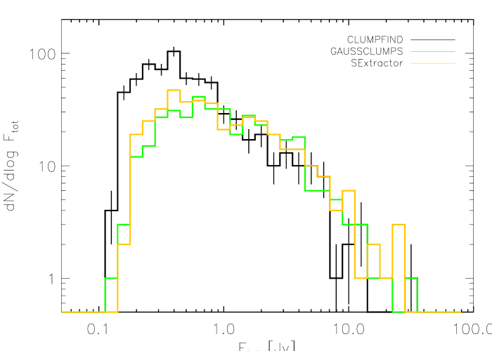
As we find an rms noise level of about 20 mJy/beam for our data we start contouring at an intensity level of $60$ mJy/beam and go in steps of $40$ mJy/beam up to $4.5$ Jy/beam, below which all the emission of the clouds is found. CLUMPFIND extracts 687 molecular clumps with a total flux of 720 Jy from the LABOCA map. This is about 63% of the total flux in the map. A section of the central region around the star cluster Tr 14, with the clumps detected by CLUMPFIND marked as blue circles, is shown in the left panel of Fig. 1. The strong point-like source $\eta$ Car has been excluded from this and the following samples. Fig. 2 shows the distribution of the extracted total fluxes $F_{tot}$.

2.2.2 GAUSSCLUMPS

GAUSSCLUMPS (GC) (Stutzki & Guesten 1990) is a least square fitting algorithm, that assumes the clumps to have a Gaussian shape and works directly on the continuous intensity distribution of the data. It first searches for the highest intensity peak on the data map and fits a Gaussian shaped clump around it. Then the algorithm subtracts the clump from the original map generating a new map on which it continues with the next iteration step.

The GAUSSCLUMPS algorithm calculates an rms noise level of 22 mJy/beam, and we define a detection threshold of $3\,\sigma$, so we can compare the results. 371 clumps are detected, only about half the number found by CLUMPFIND (see Fig. 1, middle panel; Fig. 2). Nevertheless, the total flux of 728 Jy within these clumps, is nearly the same as for the CLUMPFIND clumps.

2.2.3 SExtractor

The third algorithm we used to analyse the data is the SExtractor (SE) software from Bertin & Arnouts (1996), which originally was developed to detect stars and galaxies in large surveys. However the algorithm has also been used to extract sources in sub-mm observations of molecular cloud structures (Schuller et al. 2009; Coppin et al. 2000). Like the CLUMPFIND algorithm it uses the thresholding method to locate the clumps. To deblend sources the algorithm contours them at 30 exponentially spaced levels between the peak values of the detected sources and the detection threshold and follows the structure downwards. At each of this levels it tests if there is another peak, with an intensity exceeding a certain fraction of the total intensity. If this is the case, it extracts a new source. For each pixel between maxima, SExtractor calculates its contribution to each object by assuming a Gaussian profile, and converts this into a probability for that pixel to be assigned to a certain object.

SExtractor determined an rms noise level of about 30 mJy/beam so we used a detection threshold of $2\sigma$ to make our results comparable to the other algorithms. Corresponding to our resolution we defined the minimal area of a detected clump to 10 pixel. SExtractor finds 432 sources (see Fig. 1, right panel; Fig. 2) with a total flux of 823 Jy, 72% of the total flux in the map. This is slightly higher than the results of the other algorithms.

All the extracted sources of the SExtractor sample, as well as the clumps identified by the former algorithms, have fluxes above $1.6$ Jy/beam, except 18 of them that we considered artefacts and do not further take into account in our analysis.

2.3 Common Sources

Figure 3: The relative difference of the GAUSSCLUMPS (green) and SExtractor (yellow) fluxes with respect to the CLUMPFIND fluxes of the 38 commonly identified clumps.

The three used extraction algorithms are working along different principles. While CLUMPFIND assumes no specific clump profile, the other two algorithms presume a Gaussian shape. Furthermore the CLUMPFIND and SExtractor algorithms use thresholding methods, while the GAUSSCLUMPS algorithm works on residual maps.

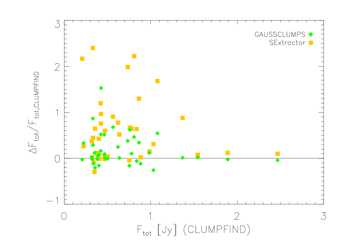
In order to check how well the extraction results of the different algorithms agree, we defined a sample of “common sources”, where the same clump is detected by all three algorithms. In the crowded and filamentary clouds in the center of the Carina nebula, many clumps are blended; therefore, the different algorithms produce often quite different decomposition results.

However, in the less crowded parts of our map, we could identify 38 rather isolated clumps which are detected by all three algorithms in a consistent way. For these, we compare the derived total fluxes in Fig. 3, where we plot the relative difference of the GAUSSCLUMPS and SExtractor fluxes with respect to the CLUMPFIND fluxes. The plot shows a generally reasonable agreement, although differences by factors up to $\sim 2-3$ are seen in the total fluxes for some of the faintest clumps in the common sample. For the majority of the clumps the deviations are less than 50%, and for most of the brighter clumps very good agreement, with deviations of less than 10%, is found. From this we conclude that for sufficiently bright isolated clumps the three extraction algorithms yield consistent total fluxes.

3 Results and Discussion

3.1 Determination of clump temperatures and masses

The masses of clumps can be calculated from the observed sub-mm flux of thermal dust emission, which is optically thin, via

$$M=\frac{d^{2}\,F_{\nu,\,\mathrm{tot}}\,R}{B_{\nu}(T_{d})\;\kappa_{\nu}}\;\;,$$ (1)

where $F_{\nu,\,\mathrm{tot}}$ is the observed spectral flux integrated over the source and $d$ is the distance of the molecular cloud. For the gas-to-dust mass ratio $R$ and the dust emissivity $\kappa_{\nu}$ we used the values from Schuller et al. (2009) i.e. $R=100$ and $\kappa_{870\,\mu{\rm m}}=1.85\,{\rm cm}^{2}\,{\rm g}^{-1}$. $B_{\nu}(T_{d})$ is the Planck function for a given dust temperature $T_{d}$ (see also Preibisch et al. 2011c).

A difference in temperature of only a few degrees in the relevant regime can change the derived masses of the clumps by a factor of $2-3$ and therefore strongly affect the derived ClMF of the region (Stamatellos et al. 2007). Hence, for a reliable mass estimation a good approximation of the temperatures of the clumps is indispensable.

Unfortunately, for single-wavelength data sets (such as our LABOCA map) no direct determination of the cloud temperature is possible. In many investigations it is assumed that all clouds in a map would have a common temperature, e.g. 15 K (e.g. Mookerjea et al. 2004; Kirk et al. 2006). While this may be a reasonable approximation in the case of more or less isolated clouds in a quiescent environment, we believe that such an assumption is not valid in the case of the Carina Nebula. The clumps in different parts of the complex will be affected by strongly different levels of irradiation, depending on the physical distance from the nearest massive stars, and this should lead to considerable differences of the cloud temperatures.

In general, clouds with high column density should be cooler than low-column density clouds, because their interior is better shielded from the external radiation field. Such a relation between column density and cloud temperature has been observed in several cases, and can provide us with important information for an estimation of cloud masses. Peretto et al. (2010) recently determined the temperatures and the column densities of a sample of 22 infrared dark clouds (IRDCs) from the Hi-GAL Galactic Plane survey (see Molinari et al. 2010) by analyzing their spectral energy distributions. Their Fig. 6 shows the expected anti-correlation between column density and temperature. To quantify this relation, we used their column density peak data, performed an Ordinary Least Squares (OLS) Bisector fit (Isobe et al. 1990) and found the relation

$$\log N_{\rm H_{2}}[{\rm cm^{-2}}]=25.6-0.22\,\log T_{d}[{\rm K}].$$ (2)

Since the column density of a clump with a dust temperature $T_{d}$ is given by

$$N_{\rm H_{2}}=\frac{F_{\nu,\,\mathrm{max}}\,R}{B_{\nu}(T_{d})\;\Omega\;\kappa_{\nu}\;\mu\,m_{\rm H}}\;\;,$$ (3)

where $F_{\nu,\,\mathrm{max}}$ is the spectral peak flux, $\Omega$ is the beam solid angle, and $\mu$ is the mean molecular weight, we have two equations relating the observed flux, column density, and temperature. We can now solve for the temperature for which the column density computed from Eq. (3) is closest to the relation in Eq. (2).

Figure 4: The distribution of individual clump temperatures (top) and column densities (bottom), with statistical errors, as found from Eq. (3) and Eq. (2) for the three different clump-finding algorithms.

Figure 5: The temperatures and fluxes of the CLUMPFIND sample, overplotted on the LABOCA map. The color of the circles corresponds to the calculated temperatures and the size of the circles to the measured flux ($\sim 2-373$ Jy/beam). The position of $\eta$ Car is marked by the black star. The black box represents the region shown in Fig. 1, centred around Tr 14 (RA(J2000)=161°, Dec (J2000)=-59°.6).

This gives us two solutions, from which we can reject the first one as it leads to temperatures below 4 K. The second solution gives us, for all samples, temperatures between $8.5-18.5$ K, which are typical values for molecular clouds and clumps (Bergin & Tafalla 2007). Most of the clumps (CF: 92 %, GC: 86 %, SE: 87 %) have temperatures above 14 K (see Fig. 4, top panel). The column density distributions we derive for the different samples are shown in the bottom panel of Fig. 4.

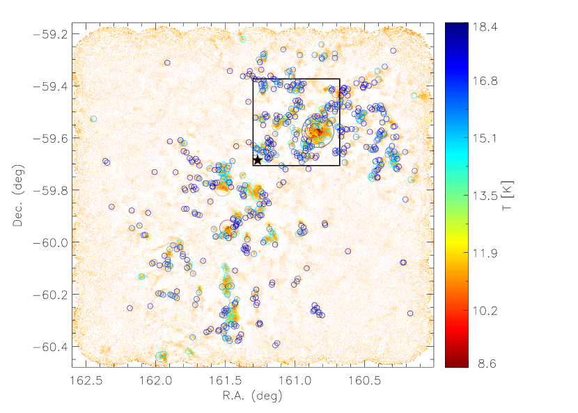
In Fig. 5 we show the location and the temperature of the clumps extracted with CLUMPFIND. The clump temperatures are shown by the color while the size of the circles increases with the measured flux $F_{\nu,\,\mathrm{tot}}$ (see also Fig. 2). The clumps are assembled along filamentary structures and pillars. These pillars show cold dense clumps on their tips, within which star formation occurs. Most of the brightest clumps are located within the structures a few arcminutes to the west of the Tr 14 cluster, where the clouds are dense and massive. The ionizing radiation of the nearby cluster can only affect the cloud surfaces and does not pervade to the cool center of the cloud.

3.2 The Clump Mass Function (ClMF)

With these individual clump temperature estimates we now can derive the masses of individual clumps. We find masses between about $5\,M_{\odot}$ and $4.7\times 10^{3}\,M_{\odot}$ and the total mass extracted in clumps is about $42\times 10^{3}\,M_{\odot}$ (see Table 1).

Figure 6: The mass histograms derived with the three different clump-finding algorithms CLUMPFIND (top), GAUSSCLUMPS (middle) and SExtractor (bottom). The black lines show the samples and their power-law slopes with the temperatures derived from the relation we got from Peretto et al. (2010). The dashed gray line shows the used lower cut-off limit for these samples. For the red line we assumed a constant temperature of 10 K for all clumps. If we assume a constant temperature of 20 K the slope does not change, but the mass distribution is shifted to lower masses (blue arrow).

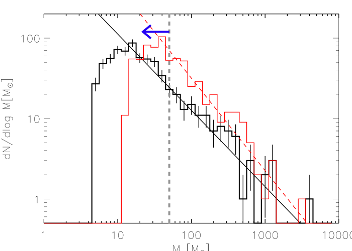
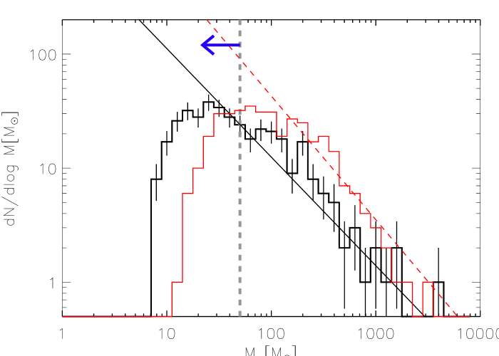
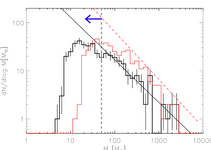
For the differential Clump Mass Function (ClMF) we plot the number of clumps $dN$ within a logarithmic mass interval $d\log(M)$ against the mass. Up to $\sim 10\,M_{\odot}$ our sample is not complete due to the mass sensitivity limit and the wide range of background levels at different locations in our map. For clump masses above $\sim 10-20\,M_{\odot}$ one can see the expected decrease in the number of clumps for rising clump mass, which roughly follows a power-law

$$\frac{\mathrm{d}N}{\mathrm{d}M}\propto M^{-\alpha}.$$ (4)

To derive the slope of the power-law tail of the mass spectra, we use the method of Maschberger & Kroupa (2009) to fit the distribution. They use a bias-free Maximum Likelihood (ML) estimator to determine the power- law exponent without binning. This method takes into account data only above a given lower cut-off limit to calculate the power-law index. In order to make sure that the fit is not affected by incompleteness effects at lower masses, we use a conservative lower cut-off limit at $50\,M_{\odot}$ (gray dashed line in Fig. 6) for the fit. For the power-law index we find $\alpha_{CF}=1.95\pm 0.07$, $\alpha_{GC}=1.95\pm 0.06$ and $\alpha_{SE}=1.89\pm 0.06$ for the CLUMPFIND, GAUSSCLUMPS and SExtractor samples, respectively (see Table 1).

3.3 ClMF assuming constant cloud temperature

A difference in temperature of only a few degrees can change the derived masses of the clumps significantly. Here we investigate how the ClMF depends on the estimated temperature. For comparison we therefore, also computed clump masses based on the assumption of isothermal clouds and considered two different values for the cloud temperature, 10 K and 20 K. These values are often assumed in sub-mm studies of molecular clouds (e.g. Johnstone et al. 2000; Kirk et al. 2006; Schuller et al. 2009). If we assume constant temperatures for all clumps the overall shape of the ClMFs keeps the same, but we derive a steeper power-law slope (e.g. for 10 K $\alpha_{CF}=2.15\pm 0.08$, $\alpha_{GC}=2.08\pm 0.06$ and $\alpha_{SE}=1.99\pm 0.06$ for a lower cut-off limit of $100M_{\odot}$). The slopes for the two different constant temperatures stay the same within their errors, as a change of temperature corresponds to a constant shift in mass (Fig. 6). The masses range between about $4\,M_{\odot}$ and $1\times 10^{3}\,M_{\odot}$ for 20 K and about $14\,M_{\odot}$ and $3.3\times 10^{3}\,M_{\odot}$ for a temperature of 10 K. The results are summarized in Table 1.

Table 1: The masses and power-law indices for the CLUMPFIND, GAUSSCLUMPS and SExtractor samples

	#	$M_{tot}$	$M_{max}$	$M_{min}$	$M_{peak}$	$\alpha$
		$[10^{3}\,M_{\odot}]$	$[M_{\odot}]$	$[M_{\odot}]$	$[M_{\odot}]$
	individual clump temperatures; lower cut-off limit: $50M_{\odot}$
CF	687	42.2	4 652.2	5.2	15.8	$1.95\pm 0.07$
GC	371	42.6	4 458.2	8.2	25.1	$1.95\pm 0.06$
SE	414	48.2	2 972.8	5.7	15.8	$1.89\pm 0.06$
	T=10K; lower cut-off limit: $100M_{\odot}$
CF		69.1	3 366.2	14.7	39.8	$2.15\pm 0.08$
GC		69.9	3 225.9	14.6	63.1	$2.08\pm 0.06$
SE		78.8	2 676.9	15.4	39.8	$1.99\pm 0.06$
	T=20K; lower cut-off limit: $32M_{\odot}$
CF		21.0	1 024.4	4.5	12.6	$2.14\pm 0.08$
GC		21.3	981.6	4.5	20.0	$2.06\pm 0.06$
SE		24.0	814.6	4.7	12.6	$2.02\pm 0.06$

Figure 7: The mass distribution of the CLUMPFIND sample with its power-law slope ($\alpha=1.95$) in black. In green the GAUSSCLUMPS sample is over plotted with its log-normal fit. The dashed gray line shows the lower cut-off limit.

3.4 Power-law versus Log-normal

Peretto & Fuller (2010) found, for a sample of gravitationally bound IRDCs, a power-law index $\alpha\sim 1.8$, while the slope of the mass spectra of unbound fragments steepens at the high mass end. They also show that the mass function of the fragments can be well described by a log-normal distribution. These results are in agreement with the theoretical work of Hennebelle & Chabrier (2008) and with studies of the probability distribution function of the column density (N-PDF) within molecular clouds which displays log-normal shapes for turbulent structures and power-law behaviour for gravitationally dominated clouds (Kainulainen et al. 2011; Ballesteros-Paredes et al. 2011).

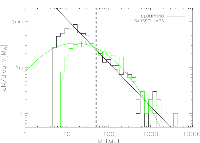
When we calculate the power-law slope for different lower cut-off limits, starting from the peak mass to higher masses, we find that the power-law index for our CLUMPFIND sample is quite robust, within the errors, regardless of whether we assume individual or constant temperatures for the clumps. The slopes of the other two samples however become continuously steeper while shifting the cut-off point to higher masses. This indicates that GAUSSCLUMPS and SExtractor samples can be also described by a log-normal function as well as by a power-law while the CLUMPFIND sample shows a clear power-law behavior (Fig. 7). We thus find that, the results of the before mentioned studies have to be used with caution while drawing conclusions on the physical state of a single molecular cloud, as the shape of the ClMF can highly depend on the clump extracting method. Whether the clumps are gravitationally bound or dominated by turbulence has to be confirmed otherwise, e.g. by determining their virial parameter (Bertoldi & McKee 1992).

4 Summary

We analysed a large-scale sub-mm map of the Carina Nebula Complex to investigate the molecular cloud structures of the region (Preibisch et al. 2011c). From this map we extract the clumps with three common clump-finding algorithms (CLUMPFIND, GAUSSCLUMPS and SExtractor) to derive the ClMF. We therefore are able to compare the resulting ClMFs and to test the influence of the extraction method and the effects of the assumed temperatures on the ClMF (see Table  1).

The assumption of a uniform temperature for the whole area disregards that the different regions within the Carina Nebula Complex are affected by highly variable levels of irradiation and stellar feedback. Hence we used an empirical calibration of the relation between column density and temperature, which we adopted from data of Peretto et al. (2010), to estimate the temperatures and masses of the individual clumps. The clump temperatures for all extraction methods lie between $8.5-18.5$ K, which are characteristic temperatures for molecular clumps.

From the subsequent resulting masses we derived the ClMFs of this region. For masses above $50\,M_{\odot}$ all samples can be described by a power-law with index $\alpha$ around 1.9, as defined in Eq. (4). This is in good agreement with the results of other studies of clump mass distributions in molecular clouds (Elmegreen & Falgarone 1996; Kramer et al. 1998; Schneider & Brooks 2004). The slope of the power-law we found is also quite similar to the slopes for cluster mass functions (e.g. Lada & Lada 2003). If we assume a uniform temperature for all clumps (10 K / 20 K) the power-law slope gets steeper.

The GAUSSCLUMPS and SExtractor samples show a lack of clumps in the low-mass range, while the CLUMPFIND algorithm finds for this mass regime at least twice the number of clumps. So even when the high mass end of the thus found ClMFs of the GAUSSCLUMPS and SExtractor samples show a power-law behaviour their overall shapes are better described by a log-normal function. The CLUMPFIND sample, however, clearly follows a power-law. Hence we find the shape of the ClMF highly dependent on the method used to extract the clumps.

Theoretical models predict that unbound turbulent clouds should have a log-normal ClMF, whereas clouds containing gravitationally bound clumps develop a power-law tail (Kainulainen et al. 2011; Peretto & Fuller 2010). In this sense, the shape of the ClMF contains very important information about the evolutionary state of a molecular cloud. However, our results show that a reliable determination of the shape of the ClMF (log-normal or power-law) is often difficult as it can depend on the specific source extraction algorithm. Therefore, conclusions drawn from a ClMF derived from a single extraction algorithm should be taken with care to avoid an over-interpretation.