The Quasar Luminosity Function from SDSS Stripe 82 ††thanks: Observations reported here were obtained at the MMT Observatory, a joint facility of the Smithsonian Institution and the University of Arizona. This paper also includes data gathered with the 6.5-m Magellan Telescopes located at Las Campanas Observatory, Chile.
Abstract
We present a measurement of the Type I quasar luminosity function at using a large sample of spectroscopically confirmed quasars selected from optical imaging data. We measure the bright end () with Sloan Digital Sky Survey (SDSS) data covering , then extend to lower luminosities () with newly discovered, faint quasars selected from 235 deg2 of deep, coadded imaging in the SDSS Stripe 82 region (the celestial equator in the Southern Galactic Cap). The faint sample includes 14 quasars with spectra obtained as ancillary science targets in the SDSS-III Baryon Oscillation Spectroscopic Survey (BOSS), and 59 quasars observed at the MMT and Magellan telescopes. We construct a well-defined sample of quasars that is highly complete, with 73 spectroscopic identifications out of 92 candidates. Our color selection method is also highly efficient: of the 73 spectra obtained, 71 are high redshift quasars. These observations reach below the break in the luminosity function (). The bright end slope is steep (), with a constraint of at 95% confidence. The break luminosity appears to evolve strongly at high redshift, providing an explanation for the flattening of the bright end slope reported previously. We find a factor of greater decrease in the number density of luminous quasars () from to than from to , suggesting a more rapid decline in quasar activity at high redshift than found in previous surveys. Our model for the quasar luminosity function predicts that quasars generate % of the ionizing photons required to keep hydrogen in the universe ionized at .
Subject headings:
quasars: general1. Introduction
The number density of quasars evolves strongly with redshift, a conclusion reached shortly after the initial identification of cosmological redshifts for quasars. Quasars increase in number with increasing redshift (Schmidt 1968) until , when quasar activity peaks, as surveys for higher redshift quasars show a steep decline in number (Osmer 1982; Warren et al. 1994; Schmidt et al. 1995; Fan et al. 2001b; Richards et al. 2006). Quasars are associated with accretion onto supermassive black holes (Salpeter 1964); how the first such black holes grew from initial seeds and were triggered by gas accretion to become luminous quasars remain key questions about the evolution of the early universe (see, e.g., the recent review by Volonteri 2010). Indeed, quasars are now observed to (Mortlock et al. 2012), indicating that the mechanisms that drive them were in place within 0.8 Gyr after the Big Bang.
The quasar luminosity function (QLF) is one of the most fundamental observational probes of the growth of supermassive black holes over cosmic time. The QLF is generally found to have the form of a broken power law (Boyle et al. 1988; Pei 1995; Boyle et al. 2000), with a steep slope towards high luminosities and a flatter slope extending to low luminosities. Observed evolution in the shape of the QLF with redshift — e.g., a change in the power law slopes or the location of the break luminosity — may provide insight into the physics of black hole growth. Many studies have found evidence for evolution of the QLF in large quasar samples (Schmidt et al. 1995; Fan et al. 2001b; Richards et al. 2006; Hopkins et al. 2007b; Croom et al. 2009). One key consequence of this evolution is the observed “downsizing” of quasar activity: where by the spatial density of more luminous objects peaks at higher redshifts (Cowie et al. 2003; Ueda et al. 2003; Hasinger et al. 2005; Croom et al. 2009).
Theoretical models for quasars have explored a variety of physical processes that may drive the triggering of quasar activity. These models make testable predictions about the evolution of the QLF based on the evolution of the triggering mechanisms. For example, models where quasar activity is instigated by mergers of gas-rich galaxies (e.g., Hernquist 1989; Carlberg 1990; Cattaneo et al. 1999; Kauffmann & Haehnelt 2000; Hopkins et al. 2006; Shen 2009) tie the QLF to the evolution of the merger rate of dark matter halos in cosmological simulations. Alternatively, some hydrodynamical simulations point to rapid inflows of cold gas along filamentary structures in the cosmic web as the primary fueling mechanism at high redshift (e.g., Di Matteo et al. 2012). It is also possible to predict the QLF while being agnostic to the specific triggering mechanisms; Conroy & White (2012) describe a model for populating galaxies with accreting black holes that directly relates the evolution of quasars to that of their host galaxies.
Furthermore, feedback from black hole accretion is expected to play an important role in regulating the growth of black holes and the duration of quasar activity (e.g., Di Matteo et al. 2005; Hopkins et al. 2006). As the QLF is a convolution of the black hole mass function and the Eddington ratio111The ratio of the mass accretion rate onto the black hole to the maximal rate allowed by the Eddington limit. distribution, these processes will alter the shape of the QLF (Hopkins et al. 2005). While the low-redshift QLF is reasonably well measured by surveys at optical, X-ray, and mid-infrared wavelengths (see, e.g., the compilation of Hopkins et al. 2007b), observations at high redshift are less constraining on these models, even though it is at high redshift where, for example, different feedback models make significantly different predictions for the quasar population (Hopkins et al. 2007a). Feedback-regulated models for quasar activity tend to predict strong evolution of the bright-end slope with redshift (e.g., Kauffmann & Haehnelt 2000; Wyithe & Loeb 2003), and also provide a physical explanation for the observed downsizing trend Scannapieco et al. (2005).
Measurements of the high redshift QLF also allow estimates of the contribution of quasars to the ionization state of the intergalactic medium (IGM) during and after reionization. Quasars are unlikely to produce enough ionizing photons to be the primary driver of reionization (Fan et al. 2001a) although current constraints on the quasar ionizing photon budget are limited to extrapolations from the bright end of the QLF and a handful of faint quasars (Jiang et al. 2009; Willott et al. 2010), as well as upper limits on moderate luminosity AGN from X-ray surveys (Barger et al. 2003; Fontanot et al. 2007). Quasars do have a much harder spectrum than stellar sources, but constraints from the soft X-ray background limit the contribution of high energy photons to large-scale reionization (Dijkstra et al. 2004; McQuinn 2012). Nonetheless, there are few observational constraints on the faint quasar population during the epoch of reionization. And while quasars may not be directly responsible for hydrogen reionization, they are expected to provide the high-energy photons responsible for He II reionization at lower redshifts (e.g., Haiman & Loeb 1998; Madau et al. 1999; Miralda-Escudé et al. 2000). Models of IGM evolution thus benefit from improved observational constraints on quasar activity at high redshift (e.g., Bolton et al. 2009).
Currently, only optical and near-IR imaging surveys provide the requisite area and depth to construct large samples of quasars at high redshifts (see, e.g., the compilation given in Ross et al. 2012). Throughout most of the 1990s, the redshift record was held by a 19th magnitude quasar at (Schneider et al. 1991). The first quasar with was discovered by Fan et al. (1999) in commissioning data from the Sloan Digital Sky Survey (SDSS; York et al. 2000). The same data were used to build a sample of 39 quasars with to a limit of (Fan et al. 2001b) and to study the evolution of quasars at high redshift, confirming the steep decline in number density at (roughly a factor of three per unit redshift). The early high-redshift quasar surveys also found evidence for flattening of the bright-end slope relative to lower redshifts (Koo & Kron 1988; Schmidt et al. 1995; Fan et al. 2001b), a result seemingly confirmed by a large, homogeneous quasar sample from the SDSS extending to (Richards et al. 2006). This form of evolutionary trend in the bright-end slope would contribute to a downsizing effect, by slowing the decline in number density with redshift for quasars above the break luminosity.
The SDSS-III Baryon Oscillation Spectroscopic Survey (BOSS; Eisenstein et al. 2011; Dawson et al. 2012) aims to collect spectra of over 150,000 quasars with redshifts between 2.2 and 3.5. Ross et al. (2012) present the QLF measured from 22,000 color-selected quasars from BOSS DR9, as well as two samples of variability-selected quasars at from Palanque-Delabrouille et al. (2011) and Palanque-Delabrouille et al. (2012). The BOSS spectroscopic target selection extends mag fainter than the SDSS, reaching below the break in the luminosity function to . Combined with the 2SLAQ (Croom et al. 2009), these large quasar surveys form a fairly complete picture of the optically unobscured (Type I) quasar population at .
At higher redshifts, over 50 quasars are now known at . While constraints at these redshifts are weaker (and await future wide-area surveys for greater numbers), the best determinations to date indicate that the bright-end slope is steep (Jiang et al. 2008; Willott et al. 2010), roughly agreeing with the measurements from BOSS and the determination from Croom et al. (2009). One of the aims of this work is to examine the QLF at intermediate redshifts and test previous claims for a flattening of the bright-end slope at .
We present a measurement of the QLF at , combining bright quasars from the SDSS with faint quasars reaching nearly 2 mag deeper. These quasars are drawn from optical imaging data (probing the rest-frame ultraviolet) and thus have low intrinsic extinction, and are confirmed by spectroscopy to be broad emission line, Type I quasars. The faint sample is derived from coadded optical imaging in the SDSS Stripe 82 region. This imaging covers to a depth more than 2 mag fainter than the SDSS main survey. The combination of medium depth and medium sky area – relative to SDSS and to small-area deep fields – is ideal for searching for rare, faint high-redshift quasars. With Stripe 82 we are able to reach sufficient depth to probe the faint end of the luminosity function, while attaining enough dynamic range to constrain its overall shape. This uniform sample of quasars — selected with simple criteria over a homogeneous imaging area — is larger than all surveys combined, and provides a key link in our understanding of quasar evolution at high redshift.

We first describe the coadded optical images on Stripe 82 that provide the primary catalogs from which we select candidates, as well as infrared imaging from UKIDSS and our own observations used to reduce stellar contamination (§ 2). Section 3 outlines our selection criteria, derived from models of quasar colors, and based on simple color cuts. We combine spectroscopy from the SDSS and BOSS surveys with our own observations using the MMT and Magellan telescopes to build a sample of over 70 quasars to a limit of ; the observations and data processing are presented in section 4 and the catalog of quasars is provided in section 5. In section 6 we use our quasar color model to quantify the completeness of the survey; with this in hand we calculate the binned luminosity function and derive a parametric form for the luminosity function using the maximum likelihood technique. We explore the evolution of the QLF at high redshift and determine the contribution of quasars to the ionizing background at based on our QLF model. We present conclusions in section 7.
We incorporate photometric data from several sources in this work; for consistency, all magnitudes are converted to the AB system (Oke & Gunn 1983) unless otherwise noted. SDSS reports photometry on the asinh scale (Lupton et al. 1999), which is nearly identical to AB at bright magnitudes. Although we use SDSS photometry only for bright quasars, we will note any instances where the asinh system is used. We refer to the SDSS DR7 imaging as “SDSS main”, in contrast to the deep imaging we use to build our primary faint quasar sample, referred to as “Stripe 82” or “the coadd imaging” (§2.1). UKIDSS magnitudes are Vega-based, but we convert all UKIDSS magnitudes to AB using the values given in Hewett et al. (2006). All magnitudes are corrected for Galactic extinction (Schlegel et al. 1998) unless otherwise noted. We use a CDM cosmology with parameters , , , and (Komatsu et al. 2009).
2. Imaging Data
2.1. Stripe 82 coadded imaging
Over the ten year duration of the survey, the SDSS I/II repeatedly imaged a 25 stripe centered at zero declination in the Southern Galactic Cap (Abazajian et al. 2009). This repeat imaging increased in frequency during the latter part of operations as part of the SDSS Supernova Survey (Frieman et al. 2007). By the end of operations, over 100 repeat imaging scans were obtained along Stripe 82 (its designation according to the survey geometry, Stoughton et al. 2002). As with the main survey, the imaging was obtained with a drift-scan camera (Gunn et al. 1998) mounted on the 2.5m Sloan telescope (Gunn et al. 2006), with nearly simultaneous 54.1 s exposures in five broad optical bands (; Fukugita et al. 1996). The quality restrictions applied to the main survey imaging (photometric and good-seeing conditions; Ivezić et al. 2004; Hogg et al. 2001) were relaxed for the Supernova Survey in order to increase the temporal coverage, resulting in a greater range of data quality.
Jiang et al. (2009) describe deep images of Stripe 82 constructed from the coaddition of 50-60 individual imaging scans at each position on the sky. Images with seeing poorer than 2″ or an -band sky background brighter than 19.5 mag arcsec-2 were rejected. The remaining images were weighted by their transparency, seeing, and sky background noise, and coadded using the SWARP software (Bertin et al. 2002). The final coadded images reach a depth roughly 2 mag fainter than single-epoch SDSS images, and were used to discover quasars as faint as (Jiang et al. 2009). These data are not the only coadded images available for Stripe 82: Annis et al. (2011) produced coadded images made using a similar process but with stricter image quality criteria resulting fewer imaging scans used at each sky position, while Huff et al. (2011) created image stacks optimized for weak lensing shear studies.
Our starting point is the coadded images from Jiang et al. (2009), which we now extend to include the and bands (Jiang et al., in preparation). The deep imaging in the bluer SDSS bands is being used to discover ultra-luminous Lyman break galaxies at (Bian et al., in preparation). In this work, we extend the Jiang et al. (2009) search for faint, quasars to lower redshifts (), as the deep -band photometry combined with the redder bands allows reliable color selection of quasars in this redshift range. The depth of our coadds is similar to that of the Annis et al. (2011) coadds (see their Fig. 7); however, as described in §4.2 we encountered much greater contamination when using the catalogs from the Annis et al. (2011) coadds for quasar selection.
We use Sextractor (Bertin & Arnouts 1996) to produce object catalogs from the deep images. Object detection was performed in the -band, and fluxes and other measurement parameters in the other bands were derived from apertures centered on the -band object position using the dual-image mode of Sextractor. All fluxes and magnitudes from the coadded Stripe 82 imaging quoted in this work are taken from aperture photometry using a 1.8″ diameter. The typical seeing in the coadded images222The weighting scheme used when coadding the images favors better seeing data; it is , where is the transparency, FWHM is the full width at half-maximum of the point-spread function (PSF), and is the variance of the sky background (Jiang et al. 2009). is 1.4″, 1.3″, 1.1″, 1.0″, and 1.1″ in , , , , and , respectively.
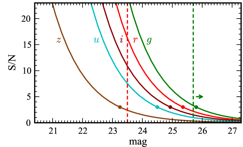
The geometry of the Stripe 82 coadded imaging follows that of the parent SDSS imaging333The SDSS camera consists of six columns of CCDs that are continuously exposed in a drift-scan mode (Gunn et al. 1998). The gaps between the CCD columns are filled by combining two Strips offset in declination (each consisting of a single scan) to form a Stripe. Thus the declination axis of Stripe 82 is split into 12 columns during the imaging scans. Each scan is 13′ wide in declination, broken into 10′ segments along right ascension; these image segments are referred to as fields.. We photometrically calibrated individual fields in the coadded catalogs by deriving zero points from the übercalibrated (Padmanabhan et al. 2008) SDSS DR8 (Aihara et al. 2011) photometry (derived from the best individual imaging scan at each location in Stripe 82), using stars with . We thus tie the aperture photometry from Sextractor on a field-by-field basis to PSF photometry from SDSS. This process results in zero points that account for seeing and photometric variations between the fields, but not within the fields. However, the large number of images contributing to the coadds tends to average over effects such as varying sky backgrounds and PSF shapes. In general, we find the photometry is highly consistent between fields and agrees quite well with SDSS photometry for the brighter objects. Figure 1 shows that the depth across the Stripe is highly uniform, and Figure 2 shows the depths reached in the bands in the coadded imaging.
Quasars at have similar fluxes in the and bands. We adopt the -band as our detection band as it provides greater a greater signal-to-noise ratio. However, at the Ly emission line and the Ly forest are within the -band. The fluxes in the band that defines our detection threshold are thus subject to the substantial variances in Ly equivalent widths, the incidence of strong Ly absorption systems, and variations in the mean IGM opacity. The -band is less affected by these issues (although it does contain C IV in emission); however, it is significantly noisier than the -band because of lower CCD sensitivity and a higher sky background. We will discuss these issues further in §5.

We further note that our survey is restricted to less than the full area on Stripe 82 for two reasons. At the time that we performed target selection, the coadds corresponding to the two uppermost camera columns had problems with the sky background in the -band, rendering them inadequate for our purposes. We thus imposed a cutoff of when selecting candidates. In addition, the western edge of Stripe 82 (near 20h) approaches the Galactic plane. Attempting color selection of quasars in this region would result in overwhelming stellar contamination (see, e.g., Figure 1 of Vanden Berk et al. 2005). We thus restrict our survey to objects with R.A. (this region also lies outside the UKIDSS imaging area described in the next section). The final area of the deep imaging we used for quasar selection is , extending from to , and from to (Fig. 1).
2.2. UKIDSS
The UKIRT Infrared Deep Sky Survey (UKIDSS; Lawrence et al. 2007) consists of multiple infrared imaging surveys with the UKIRT Wide Field Camera (WFCAM; Casali et al. 2007), including a wide-area component (the Large Area Survey or LAS) that covers to a depth of (). The LAS includes Stripe 82, providing shallow infrared imaging of our candidates and additional leverage in discriminating high redshift quasars from stellar contaminants. We first apply a loose color cut to identify potential quasar candidates from the coadded optical imaging,
then queried the DR8plus release in the WFCAM Science Archive (WSA; Hambly et al. 2008) for infrared counterparts.
Quasars at have (see section 3), thus at the faint limit of our survey most of our target objects do not have a counterpart in the UKIDSS catalogs. However, stars with similar optical colors to quasars (namely, M and L dwarf stars) are redder in the near-IR (, see Fig. 5) and thus are relatively brighter at infrared wavelengths. We downloaded -band image cutouts from the WSA for all of the candidates pre-selected from the optical imaging, then performed aperture photometry using the IRAF aper task at the -band position from the SDSS coadded imaging, measured in 2″ diameter apertures. We validated our photometry by checking against the UKIDSS catalog measurements for brighter objects (utilizing the UKIDSS calibration as described in Hodgkin et al. 2009). The aperture photometry reaches at , sufficient to discriminate the typical stellar contaminants at our limit of .
2.3. MMT SWIRC
At the time the initial candidate selection was performed, the publicly available UKIDSS data on Stripe 82 did not extend to R.A. . We imaged some of the candidates lacking coverage on 2011 Oct 14-15 with the MMT Smithsonian Widefield Infrared Camera (SWIRC; Brown et al. 2008). Each object was observed in the band using a 9-point dither pattern with 30s exposures at each position, for a total integration time of 4.5 min. The typical seeing was 0.6-0.9″. Images were dark-corrected, flat-fielded, sky-subtracted, shifted, and combined using standard IRAF routines. Object photometry was measured in 2″ diameter apertures using IRAF routines, and calibrated using observations of UKIRT Faint Standards.
A total of 38 objects were observed with SWIRC. This includes 10 objects already spectroscopically confirmed as quasars but that lacked UKIDSS coverage or had low in the -band. These objects were observed as a check on our -band color selection for quasars selected solely by optical colors. The remaining SWIRC targets were taken from a sample of objects selected as high-redshift quasar targets based on optical colors but that lacked UKIDSS coverage. These objects are mainly at , the region of our survey with the highest stellar density. Nearly all of these sources were readily identified as stellar contaminants from bright detections in the SWIRC imaging, and would have greatly reduced the purity of our spectroscopic sample had they not been observed with SWIRC.
Figure 3 displays postage stamp images of a typical quasar within our survey. The -band clearly has the highest . The non-detection in UKIDSS and the faint detection in the deeper SWIRC imaging are expected for a quasar; a contaminating star would have been easily identified from the infrared imaging.
3. Quasar Candidate Selection

Quasars are typically selected from imaging data using their colors, but these colors are a strong function of redshift, and overlap with the stellar locus at certain redshifts (Fan 1999; Richards et al. 2001, 2002). Optimal techniques have been developed for extracting the much rarer quasar population from the overwhelming contamination due to stars within the Galaxy. The probability that an object is a quasar or star can be determined by considering the local density of quasars and stars in the multidimensional space defined by the set of fluxes available from an imaging survey. These probabilities can be used to efficiently select quasar candidates (Bovy et al. 2011; Kirkpatrick et al. 2011). Similar techniques have also been applied at high redshift, where the problem is worsened by the extreme rarity of quasars and the small number of bands in which the candidates are detected, typically at low (Mortlock et al. 2012).
Fortunately, at quasar colors are well separated from those of stars. At the -band is completely within the Ly forest and the colors of quasars shift markedly redward of the stellar locus, while the colors sample the Ly to C IV region of the rest-frame UV and are bluer than the stellar locus. The -band samples the Lyman limit; colors are generally redder than those of stars due to the mean forest absorption; furthermore, most quasars will encounter a Lyman Limit System (LLS) near the red edge of the -band, leading to saturated absorption and a -band non-detection. Simple color selection at these redshifts was used in the SDSS I/II (Richards et al. 2002), leading to the first quasars discovered at (Fan et al. 1999) and a total of over 300 quasars by the DR7 release (Schneider et al. 2010).
In this section, we describe a model for quasar colors based on simulated quasar spectra. We use these model quasar colors to motivate our simple color cuts that achieve a high degree of both completeness and purity.
3.1. Simulated quasars
Fan (1999) outlines a procedure for generating simulated quasar spectra using a simple empirical model for their spectral properties at UV/optical wavelengths. The simulated spectra are integrated through survey bandpasses to generate simulated fluxes (colors) that can be used to define selection criteria, and to estimate their completeness. This requires that the spectral model reliably captures the diversity of quasar spectral features, and thus accurately reproduces observed quasar colors. The basic components of the quasar model are a broken power-law continuum, prominent UV/optical emission lines, pseudo-continuum from Fe complexes, and redshift-dependent Ly forest absorption due to intervening neutral hydrogen. We have used an updated version of this model (described below) to reproduce the colors of quasars from the SDSS-III/BOSS in the range (Ross et al. 2012). We apply the model at higher redshift under the assumption that the distribution of quasar SEDs does not evolve with redshift (Kuhn et al. 2001; Yip et al. 2004; Jiang et al. 2006). This approach can be compared to, e.g., cloning the spectra of lower redshift quasars to higher redshift (Chiu et al. 2005; Willott et al. 2005), which carries with it any selection function imprinted on the lower redshift sample; or using a small set of quasar templates (Mortlock et al. 2012), which may not capture objects with unusual features.
Each quasar is assigned a power law continuum with a break at 1100 Å. The blue slope is drawn from a normal distribution with and (Telfer et al. 2002)444Using a larger sample of quasars with HST Cosmic Origins Spectrograph observations, Shull et al. (2012b) derived a far-UV slope of and a break wavelength at 1000 Å. We kept the softer slope from Telfer et al. (2002) for consistency with the BOSS analysis. At the far-UV colors are dominated by Ly forest absorption; thus the slight change in slope will have little effect on quasar selection.; the distribution for the red slope is and . We add to this continuum emission lines with Gaussian profiles, where the Gaussian parameters (wavelength, equivalent width, and FWHM) are drawn from normal distributions. These distributions are derived from fitting composite spectra of BOSS quasars in luminosity bins. These distributions recover trends in the mean and scatter of the line parameters as a function of continuum luminosity, e.g., the Baldwin Effect (Baldwin 1977), and blueshifted lines (Gaskell 1982; Richards et al. 2011). Finally, we include Fe emission using the template of Vestergaard & Wilkes (2001), scaling the template in segments to match the Fe emission in the composite spectra. We do not include a contribution from quasars with unusually weak emission lines, which account for % of quasars at (Diamond-Stanic et al. 2009), or from Broad Absorption Line (BAL) quasars, which tend to have moderately redder colors (e.g., Weymann et al. 1991; Brotherton et al. 2001; Reichard et al. 2003).

The quasar model for the BOSS employs a prescription for the Ly forest based on the work of Worseck & Prochaska (2011). This forest model is calibrated to observations at . We extend the model to higher redshifts by using the observed number densities of high column density systems from Songaila & Cowie (2010). For the lower column density systems (), we begin with the parameters of Worseck & Prochaska (2011), and follow their method of deriving the number densities by simulating a large number of sight lines and matching the mean free paths (mfps) of the simulated sightlines to the observations of Songaila & Cowie (2010). We also force continuity between the column density distribution function () at low and high column densities, and check the derived effective optical depth () against the measurements of Songaila (2004) and Fan et al. (2006a). There remains significant uncertainty in forest parameters at high redshift, but our simple color selection method is relatively insensitive to the model for the Ly forest. To account for the degree of uncertainty in the forest absorption, we also include a “low” and “high” forest model, scaling the number densities of forest absorbers up and down by 10%, matching the scatter in measurements by Songaila & Cowie (2010). After comparison with observed quasar colors, we find that the model with a mean forest density 10% greater than the best-fit value from the mfp measurements provides the best match. Figure 4 shows an example simulated quasar spectrum from our models, and compares the Ly forest observables (mfp and ) obtained from our simulated forest spectra to observations of high redshift quasars.
3.2. Color Selection
Based on the results from the simulated spectra, we concluded that the most efficient use of telescope time was to focus on a fairly narrow redshift range, , where the colors of stars and quasars are best separated and the selection efficiency is high. Figure 5 shows the , , and colors of red stars and high redshift quasars in our sample, as well as the selection criteria we adopted:
-
•
-
•
-
•
OR
-
•
-
•
-
•
-
•
where all magnitudes are in the AB system, measured within fixed apertures (as described in §2), and have been corrected for Galactic extinction using the maps of Schlegel et al. (1998). measurements are obtained from the aperture fluxes and uncertainties given by Sextractor.
We apply no morphological criteria in our candidate selection after finding that the number of potentially resolved objects (Sextractor CLASS_STAR ) is small ( of the total selected), indicating that contamination from compact galaxies is negligible.
These criteria are similar but not identical to the cuts that define the inclusion region in the SDSS quasar selection algorithm, as given in Richards et al. (2002). We extend the selection nearly 2 mag fainter than the SDSS main survey by utilizing the coadded imaging on Stripe 82. We define dropout criteria in the and bands through criteria within fixed apertures rather than a magnitude cut. Although the Stripe 82 coadded imaging is highly uniform (e.g., Fig. 1), using a threshold more fully utilizes the -band depth at a given location, as quasars are not expected to have any detectable flux in this band. We bracket the redshift range of the search to by requiring a red color and to by requiring a blue color. Finally, we take advantage of the available infrared data from UKIDSS, effectively imposing a veto on objects that are too red in . This cut is made using the aperture flux ratios in the and bands, so that objects undetected in the UKIDSS band — as expected for quasars — pass the final cut without imposing a threshold.
The -band detection catalog contains 1.5M objects. We apply loose pre-selection cuts in the colors (see middle panel of Fig. 5 and §2.2) to reduce this list to potential candidates for which UKIDSS images are downloaded and analyzed. The near-IR photometry is highly useful as stellar veto: of the pre-selected candidates from the optical imaging, only are rejected by the color cut we adopt (§3.2) using the UKIDSS catalog photometry, while are rejected based on the aperture fluxes. After applying the final color criteria listed above, we have 92 candidates to a limit of .
4. Spectroscopic Observations and Data Reduction
We obtain spectroscopic identifications of our candidates from multiple sources by utilizing the dense SDSS/BOSS spectroscopic coverage of Stripe 82 combined with our own observations. First, we identify a few of the brightest candidates on Stripe 82 using spectroscopic data from the SDSS I/II (Abazajian et al. 2009). More recently, the BOSS collected a large number of spectra on Stripe 82, including several ancillary science programs (Dawson et al. 2012) targeting high redshift quasars. Finally, we have obtained spectra for additional candidates (extending much fainter than the SDSS and BOSS spectroscopic observations) using the MMT and Magellan telescopes. In total, we have 73 spectroscopic identifications for our 92 candidates (79%). The candidates with spectroscopic observations can be considered an unbiased subset of the full candidate sample, as will be discussed further in § 6.1. Table 1 summarizes the status of spectroscopic observations of quasar candidates on Stripe 82, including a number of confirmed quasars not within the uniform sample.
4.1. SDSS DR7
The SDSS I/II spectroscopic survey concluded with the DR7 release (Abazajian et al. 2009). Spectra were reduced with the standard SDSS pipeline (Stoughton et al. 2002). Quasar target selection is described in Richards et al. (2002); high-redshift quasars are targeted through two methods, both to a limit of . First, outliers from the stellar locus in space are identified as high-redshift quasar candidates, and second, various color cuts aim to extend the quasar yield within specific redshift ranges beyond the locus outlier selection. Schneider et al. (2010) present a catalog of over 100,000 spectroscopically confirmed quasars drawn from of the DR7 spectroscopic footprint (hereafter DR7QSO). This catalog includes 191 quasars at to a limit of , of which 184 are selected by our color criteria based on their SDSS flux measurements.
We utilize the DR7 data in several ways. First, we matched our candidate list to the DR7QSO catalog, as well as to the full DR7 spectroscopic database. We identified eight of our candidates as confirmed quasars in DR7QSO. There were three additional quasars in this redshift range that did not meet our color criteria. None of our candidates matched to non-quasars among the 1.6 million objects with spectra in DR7.
We further employ the DR7 quasars to determine the bright end of the luminosity function, by constructing a uniform sample of DR7QSO quasars in our redshift range drawn from the SDSS DR7 imaging footprint. We will describe this sample in §6.1.1.
4.2. BOSS
The BOSS quasar survey is primarily designed to find quasars at for the purpose of Ly forest studies (McDonald & Eisenstein 2007; Ross et al. 2012). The Extreme Deconvolution algorithm (XDQSO) used as the primary quasar targeting method in BOSS is tuned to this redshift range and is highly efficient (Bovy et al. 2011). However, a large section of Stripe 82 was observed by BOSS in Fall 2010 as BOSS Chunk 11 (Ross et al. 2012); during these observations quasars were targeted through a combination of color selection (using XDQSO) and variability selection (Palanque-Delabrouille et al. 2011). The highest redshift quasar identified by the main BOSS targeting in Stripe 82, including variability, is at .
In addition, we are conducting ancillary science programs in BOSS that take advantage of unused fibers once the primary survey targets (galaxies and mid- quasars) have been allocated fibers (Dawson et al. 2012). These programs extend the and color cuts described in Richards et al. (2002) to fainter quasars by utilizing areas with multiple epochs of imaging in SDSS I/II due to overlapping or repeated scans. On Stripe 82 these ancillary programs utilized photometry from the -epoch coadded images available in the DR7 CAS and described in Annis et al. (2011); these observations are included in BOSS DR9 (Ahn et al. 2012). We will analyze the quasars identified in overlap regions outside of Stripe 82 in future work.
The selection criteria for quasars are similar to the inclusion region in Richards et al. (2002), but extended to a faint limit of and using the catalogs from the Annis et al. (2011) coadded imaging for target selection. On Stripe 82, this program was allocated 283 targets, of which 221 received spectra, but only 22 were high- quasars. Of those, 10 were previously known from SDSS DR7; thus the program yielded only 12 new quasars. All 12 meet our selection criteria and are included in this study. The ancillary program targets that are not quasars fall mainly into two categories: 1) objects with fluxes contaminated by nearby bright stars, and 2) spurious or moving objects (e.g., asteroids). We matched the failed targets to the coadded image catalogs and found that either they did not have matches in our coadded imaging, or the matches did not meet our selection criteria.
BOSS spectra are collected with a fiber-fed, multi-object spectrograph (Smee et al. 2012) and reduced with a pipeline described in Bolton et al. (2012). We visually examined all of the spectra for ancillary program targets on Stripe 82, as well as any classified by the pipeline as having . We also cross-checked our examinations against the DR9 Quasar Catalog as described in Pâris et al. (2012). As with SDSS, we cross-checked our candidate list against all spectra in BOSS, not just confirmed quasars, again finding no matches to non-quasars. Figure 20 displays the BOSS spectra of quasars on Stripe 82.
| Sample | Uniform | All |
|---|---|---|
| Candidates | 92 | - |
| … spec. ids | 73 | 106 |
| … quasars | 71 | 84 |
| … | 52 | 64 |
4.3. Magellan observations
The remaining candidates on Stripe 82 () were mostly fainter than and required spectroscopic observations on larger telescopes. We first observed four candidates at the Magellan Clay 6.5m on 2011 Jun 11-13 using the Magellan Echellette spectrograph (MAGE; Marshall et al. 2008). MAGE provides full coverage from 3100Å to 1m at a resolution of using the 0.7″ slit. The typical seeing during this run was 0.6″.
Magellan spectra were reduced using MASE (Bochanski et al. 2009), an IDL-based pipeline designed for MAGE data. Wavelength calibration was provided by ThAr lamps observed shortly after the targets and at a similar airmass, and the standard star Feige 110 was used for flux calibration. Of the four targets observed at Magellan, three are quasars (Figure 21; one object had been previously observed in BOSS), and one is a star.
4.4. MMT observations
The bulk of our spectroscopic observations occurred at the MMT 6.5m telescope using the Red Channel spectrograph. We used the 270 mm-1 grating centered at 7500 Å555Some objects were observed at a redder setting during the course of a program targeting higher redshift objects., providing coverage from 5500Å to 9700Å. We used either the 1″ or 1.5″ slit based on the seeing, providing resolutions of and , respectively.
Observations were conducted on 2011 Jun 23-24, 2011 Oct 1-4, and 2012 May 27-28. During 2011 June nine objects were observed in poor seeing (1.5-3″); five were confirmed as quasars. Conditions during the 2011 October run were fair with ″ seeing; however, most of the run was lost to thick clouds and high humidity, particularly during the early part of the night. As a result, we obtained few spectra for candidates at . In total, 52 targets were observed in October, of which 41 were confirmed quasars. In the 2012 May run, 17 additional candidates with were observed, resulting in 11 new high-redshift quasars. Conditions during this run were excellent, with ″ seeing throughout. In general we valued efficiency over quality. Therefore the exposure times were short, between 5 and 15 minutes with typically a single exposure per target, and many of the spectra have a low signal-to-noise ratio. However, the quasars among the observed targets are easily identified by their prominent emission lines, while the few contaminants can be ruled out as high-redshift quasars by the lack of either emission lines or a strong spectral break towards blue wavelengths.
Data were processed using standard longslit reduction techniques through a combination of Pyraf666Pyraf is a product of the Space Telescope Science Institute, which is operated by AURA for NASA. and python routines, including bias subtraction, pixel level corrections from flat fields generated from internal lamps, and sky subtraction using a polynomial background fit along the slit direction. Cosmic rays were idntified and masked using the LACOS routines (van Dokkum 2001). Wavelength calibration was provided from an internal HeNeAr lamp, and then corrected on a per-image basis using night sky lines (primarily the OH line list given by Rousselot et al. 2000). Standard stars were observed between one and three times per night and used for flux calibration. However, the conditions were highly variable and the absolute flux calibration of the spectra is not reliable. Figure 22 shows the MMT spectra obtained for high redshift quasars on Stripe 82.
5. Quasar catalog
Table 4 consists of our full Stripe 82 quasar catalog, consisting of:
-
•
11 SDSS DR7 quasars with ,
-
•
14 BOSS DR9 quasars with ,
-
•
59 quasars with spectra obtained at MMT and Magellan.
For all objects, we provide photometry in the bands derived from the coadded imaging that formed the basis for our target selection. We also provide -band photometry obtained from our aperture photometry of the UKIDSS DR8plus images, or, when available, imaging from MMT SWIRC. The table includes all quasars on Stripe 82 from the three data sources, but not all of these quasars are included in the uniform sample used to calculate the QLF (§6). In §6.1.2 we will derive the selection probability for each quasar, this value is included in the catalog and we flag quasars that are not part of the uniform sample by assigning them a value of .
The only line widely available at a reasonable in our spectra is the Ly line. Our spectra do generally cover the C IV emission region; however, this line shows offsets from the systemic redshift that are correlated with properties such as luminosity and radio loudness (e.g., Richards et al. 2011). Therefore, we assign redshifts based on a combination of fitting the Ly line777The Ly line can also have systematic offsets, in particular a redshift due to absorption of the blue wing by the Ly forest (e.g., Shen et al. 2007). We do not account for this offset as it is much smaller than the uncertainties we assume for our redshift designations., measuring the onset of Ly forest absorption, and visually matching a quasar template spectrum to the observed spectra. In general, the redshifts have an uncertainty of , which is sufficiently accurate for calculation of a luminosity function. All of our quasars are consistent with a Type I classification based on their broad line widths ().
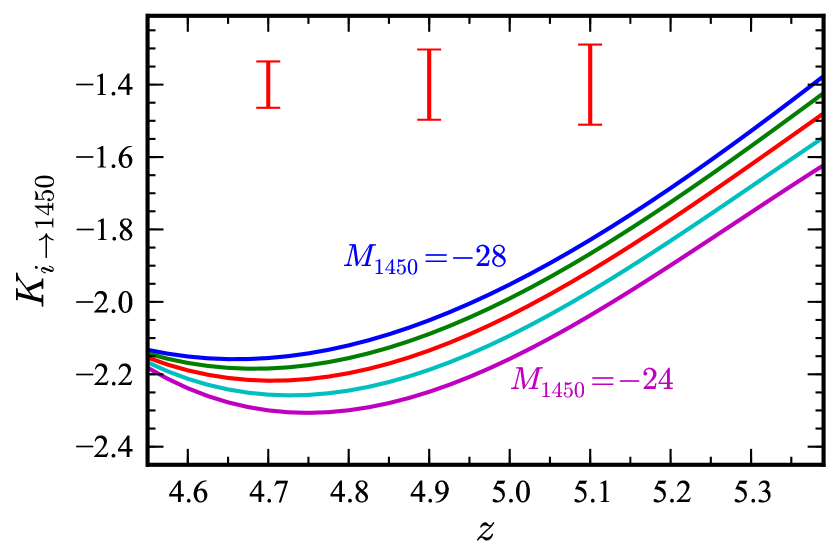
We use the simulated spectra derived from our quasar model (§3.1) to derive -corrections as a function of both redshift and luminosity. We derive the average correction for the observed -band flux to the monochromatic luminosity at rest-frame 1450 Å () for a large number of simulated quasars in narrow bins of (see §6.1), then interpolate this grid to derive an individual quasar correction. Figure 6 shows the luminosity-dependent -corrections derived from our quasar model and used in this work. Accounting for the average emission line contribution to the -correction as a function of luminosity alleviates some of the issues arising from the fact that our best photometry is in the -band, which contains the Ly line.888Note that the -band measurement is from the coadded imaging, and is thus an average of a decade of individual measurements, smoothing over the variable lightcurve of each quasar. This approach also corrects for some of the bias introduced by luminosity-dependent line emission and its effect on broadband photometric data. However, the distribution of intrinsic quasar SEDs at a given luminosity and redshift is quite broad, introducing scatter into our absolute magnitude calculations (also shown in Figure 6).
Alternatively, the -correction can be derived directly from the spectral data (see, e.g., Glikman et al. 2011, for a discussion of spectral -corrections for high quasars). However, we are again limited by the low in the continuum of our spectra. In addition, we do not attempt an accurate flux calibration of our spectra (indeed, the BOSS quasar spectra are known to have flux calibration errors in some instances, see Pâris et al. 2012). Thus we would need to calibrate the observed (noisy) spectra with the broadband fluxes from the imaging. We chose to use a template -correction based on photometry as it can be more consistently applied.
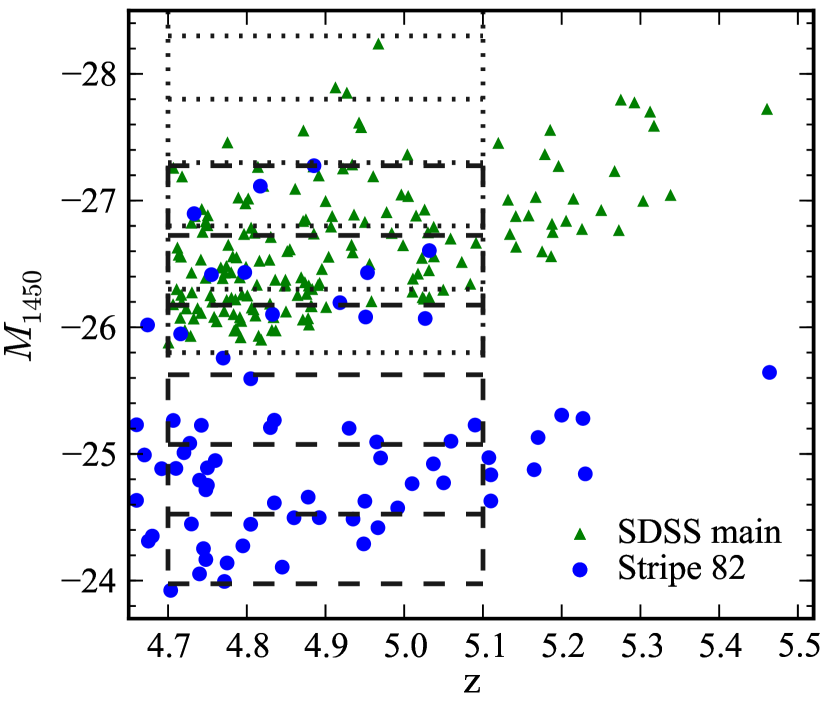
Figure 7 shows the distribution in redshift and luminosity for both the Stripe 82 and SDSS main samples, after applying our -corrections.
5.1. Notes on individual objects
In this section, we note objects that have radio detections, uncertain identifications from the spectroscopy, and unusual spectral features.
J221941.90+001256.2 (), J224524.27+002414.2 (): These two objects have radio counterparts at 1.4 GHz from VLA imaging of Stripe 82 (Hodge et al. 2011). They are the only sources with counterparts in that catalog, which is derived from imaging over 92 deg2 to a depth of 52 Jy beam-1. J221941.90+001256.2 has a peak flux density of mJy beam-1 and J224524.27+002414.2 has mJy beam-1. Both sources also have counterparts in the Faint Images of the Radio Sky at Twenty-Centimeters (FIRST) catalog (Becker et al. 1995), with peak flux densities of mJy beam-1 and mJy beam-1, respectively. Neither is included in our uniform sample as they lie outside the defined redshift range. J221941.90+001256.2 also shows strong broad absorption line (BAL) features.
J223907.56+003022.6 (), J232741.35-002803.9 (), J021043.16-001818.4 (): These three objects also have FIRST counterparts, with peak flux densities of mJy beam-1, mJy beam-1, and mJy beam-1, respectively. All three are included in the uniform sample.
J211158.01+005302.6 (), J234730.56+002306.3 (): We identified these objects as quasars based on their discovery spectra; however, the spectra are noisy and the identifications were uncertain. We later confirmed them as quasars with MMT observations on 2012 Aug 25.
J211225.39-000141.3 (), J030315.05-000347.6 (): These spectra also have low . Both objects appear to have a Lyman break feature (more evident in the 2D spectra) and Ly and N V emission features, with apparent N V absorption troughs. We include these objects as confirmed quasars. J030315.05-000347.6 may have BAL features.
J222018.48-010146.8 (), J000552.33-000655.6 (): These two quasars were targeted as part of an SDSS+UKIDSS high- BOSS quasar ancillary program. J000552.33-000655.6 was first reported in Fan et al. (2004).
6. Results

6.1. Survey Completeness
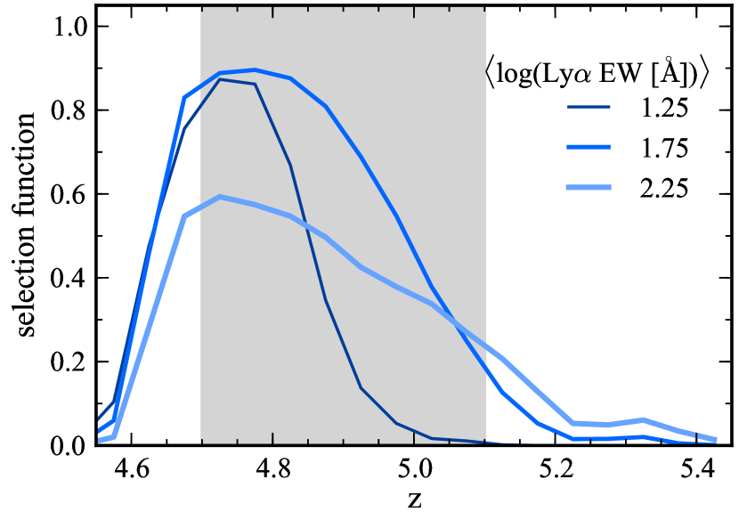
We use the simulations described in section 3.1 to estimate the completeness of our selection criteria. To derive a selection function, we construct a grid of simulated quasars distributed evenly in () space with 200 quasars per bin of , . Each object is sampled from models for quasar emission properties as outlined in § 3.1. The simulated quasars are then passed through the color cuts after adding photometric errors, and the fraction of objects within each bin that pass the cuts provides an estimate of the completeness for a given luminosity and redshift, under the assumption that our quasar model accurately represents the intrinsic distributions of quasar properties.
We generate two simulation grids. The first adopts photometric uncertainties typical of the SDSS main survey and uses asinh magnitudes; we use this simulation to derive the completeness of the SDSS quasar survey at . The second uses photometric uncertainties from the coadded imaging and is used for the Stripe 82 sample. The uncertainties are determined by fitting a relation to the uncertainties of stellar objects in the Stripe 82 catalog as a function of band flux.
6.1.1 DR7 Completeness
The SDSS quasar selection algorithm (Richards et al. 2002) was not finalized until the survey was already in progress, thus to construct a statistical sample from DR7 we follow the method given in Richards et al. (2006) to identify DR7 quasars from regions with uniform target selection. This limits the final area to . We further cut the DR7 sample to only objects selected by the color inclusion regions (excluding objects selected only as stellar locus outliers); this results in the loss of only a few objects, but greatly simplifies the calculation of the selection function. After restricting to the uniform targeting area and applying the color cuts, DR7QSO provides 146 quasars with 999We do not double-count DR7 quasars that lie on Stripe 82 when calculating the LF, as the uniform targeting area does not include Stripe 82..
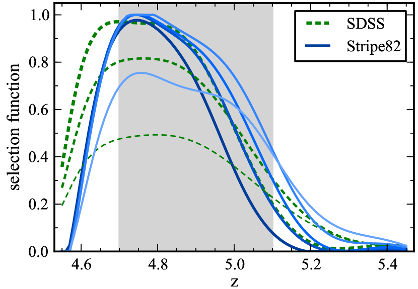
We use the simulated quasar photometry combined with the color cuts of Richards et al. (2002) to derive the selection function for quasars in the main SDSS sample (Figure 8). We add a 5% correction for photometric incompleteness (i.e., objects lost due to crowding or proximity to bright stars or galaxies, see Richards et al. 2006) and spectroscopic incompleteness of 5% (objects selected by the targeting algorithm but without a spectrum in DR7). We determined the latter incompleteness by querying the DR7 Target database for objects with the QSO_HIZ flag, finding that 5% lack spectra. The missing spectra are mainly due to fiber collisions that result when tiling spectroscopic targets, due to the restriction that fibers on a single plate must be separated by ″.
6.1.2 Stripe 82 Completeness
Although the Stripe 82 selection function is obtained from the same quasar model as for DR7, it is evident from Figure 8 that the Stripe 82 selection probes a different population. First, the Stripe 82 data are much deeper and thus the completeness remains high to lower luminosities. Also, the color selection criteria are somewhat different. Figure 9 compares the selection efficiencies for DR7 and Stripe 82 as a function of redshift. It is noteworthy that the selection function value is higher for fainter objects at some redshifts. This is because the selection function calculation averages over a range of colors in each () bin, with the colors depending on the continuum slopes, line strengths, and other features sampled from the model. At , our color selection is quite sensitive to the Ly equivalent width, as shown in Figure 10. Because the EW increases at lower luminosities and Ly is fully within the -band in our redshift range, the colors of fainter objects are redder in and bluer in than brighter objects, increasing their likelihood of meeting our selection criteria (see also Figure 5). This effect is not captured by models that do not account for the Baldwin Effect.
Our selection function models generally predict near-zero completeness for quasars; however, it is clear from Figure 7 that our color criteria do select a non-negligible number of quasars at these redshifts (particularly for the DR7 data). We found that models with increases in both the mean and scatter of the Ly EW distribution provide a better fit to the observed colors (and the redshift distribution) than our fiducial model. However, these models had little effect on our primary analysis, as we restrict to the range , where our fiducial model already predicts high completeness. We thus chose to maintain consistency with the BOSS analysis presented in Ross et al. (2012) and adopt the same quasar spectral model.
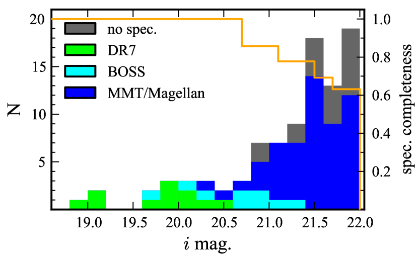
We estimate the photometric completeness to be 95% (see, e.g, Fig. 7 of Annis et al. 2011). The spectroscopic coverage of the Stripe 82 candidates is high: of candidates with have spectra. Near the faint limit, the completeness is a bit lower: 69% of candidates with and 63% of candidates with have spectra. Figure 11 shows our spectroscopic completeness as a function of observed magnitude, as well as the correction we use to account for the missing spectra in our luminosity function calculation. In total, 19 candidates do not have spectroscopic identifications; by applying this correction we assume that they are a random subsample of the full candidate set. This assumption is fair given that the choice of which targets to observe was largely constrained by sky location and weather conditions, not properties of the candidates themselves (such as color).
The Stripe 82 survey includes 52 quasars at . The Stripe 82 sample is not only highly complete but also highly pure: out of 73 candidates with spectroscopic identifications, 71 are high-redshift quasars (), and 52 (71%) are quasars in the targeted redshift range. For completeness, we provide in Table 5 a list of the candidates that were either not observed spectroscopically (19 objects), or were found not to be high-redshift quasars (2 objects, both have no emission features and appear to be stellar continua).
6.2. Binned Luminosity Function
We first calculate the luminosity function from the combined SDSS main and Stripe 82 quasar samples by dividing the sample into discrete bins of luminosity and redshift. Guided by our completeness calculations, we restrict the sample to the interval , where the selection efficiency is relatively high. We refer to this as the uniform sample. We use a single redshift bin, ignoring any evolution of the QLF parameters over the width of the bin. In particular, the redshift evolution derived by Fan et al. (2001b) predicts a decline by a factor of in space density from to . We do not account for this evolution in the binned QLF, but it will be incorporated below in a maximum likelihood fit to each quasar. We calculate the binned luminosity function using the method (Schmidt 1968; Avni & Bahcall 1980), including the correction of Page & Carrera (2000). The calculation is performed separately on the DR7 and Stripe 82 data, accounting for the differences in sky area, depth, and selection criteria between the two samples.
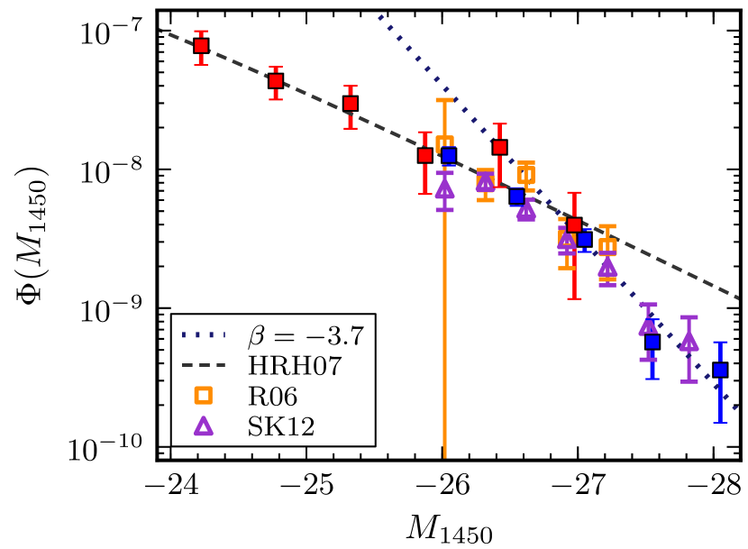
Table 2 provides the binned QLF for both the SDSS main (DR7) and Stripe 82 samples. We include the number counts in each magnitude bin, as well as the corrected number counts after accounting for all sources of incompleteness. The binned QLF data is also displayed in Figure 12. The SDSS data show a steep drop in the number density at the bright end; from the combined data it is evident that the QLF becomes shallower towards lower luminosities. Fitting a single power law to the binned data from both surveys at the bright end () results in a steep slope of .
Shen & Kelly (2012) have also calculated the binned QLF of SDSS quasars at , repeating the DR3 analysis of Richards et al. (2006) for the larger DR7 sample. Our methodology differs from that of Shen & Kelly (2012) in several respects. Most notably, we have recalculated the selection function and -corrections using our new quasar model. In addition, we restrict the quasar sample to color-selected objects (excluding those identified only as stellar locus outliers). The Richards et al. (2006) selection function has a value of at , much higher than the values we obtain (see Fig. 9), and inconsistent with our previous finding (§6.1.1) that few quasars were selected by locus outlier criteria alone. However, although our selection function disagrees with that of Richards et al. (2006) by as much as a factor of at , the highest redshift bin () in both Richards et al. (2006) and Shen & Kelly (2012) is dominated by objects near the low redshift edge of the bin. Finally, we use a slightly different method for calculating the spatial area of the survey; however, we obtain a similar result ( vs. ). Figure 12 compares our binned QLF to Richards et al. (2006) and Shen & Kelly (2012); the agreement is generally good, though differences of % may still be attributed to the different approaches used.
| aa is in units of Mpc-3 mag-1. | bb is in units of Mpc-3 mag-1. | |||
|---|---|---|---|---|
| DR7 | ||||
| -28.05 | 3 | 4.8 | -9.45 | 0.21 |
| -27.55 | 5 | 7.7 | -9.24 | 0.26 |
| -27.05 | 30 | 42.0 | -8.51 | 0.58 |
| -26.55 | 57 | 85.1 | -8.20 | 0.92 |
| -26.05 | 51 | 81.5 | -7.90 | 1.89 |
| Stripe 82 | ||||
| -27.00 | 2 | 2.2 | -8.40 | 2.81 |
| -26.45 | 5 | 8.1 | -7.84 | 6.97 |
| -25.90 | 5 | 7.0 | -7.90 | 5.92 |
| -25.35 | 10 | 16.7 | -7.53 | 10.23 |
| -24.80 | 15 | 24.3 | -7.36 | 11.51 |
| -24.25 | 14 | 26.8 | -7.14 | 19.90 |
6.3. Parameter Estimation From Maximum Likelihood
| aa, with . | |||
|---|---|---|---|
| -4.00 | |||
| -1.50 | |||
| -26.39 | -1.80 | -3.26 |
Note. — Parameters without uncertainty ranges are fixed during the maximum likelihood fitting.
We now derive parametric fits to the observed data using maximum likelihood estimation. The maximum likelihood estimate for a luminosity function corresponds to the minimum of the log likelihood function
where the first sum is over the observed quasars, and the second is over the full luminosity and redshift range of the sample and provides the normalization (Marshall et al. 1983, see Fan et al. 2001a and Kelly et al. 2008 for alternative derivations of the likelihood function). The term is the probability that a quasar with absolute magnitude (for our purposes, ) and redshift is included in the survey; i.e., the selection function as derived in section 6.1, including all sources of incompleteness. Confidence intervals are derived from the likelihood function using a distribution in (Lampton et al. 1976).
Over a wide redshift range, the quasar luminosity function is found to be well fit by a double power law (Boyle et al. 1988),
where is the characteristic luminosity at which the function changes slope from steep at the bright end () to shallow at the faint end (). The four QLF parameters may evolve with redshift, possibly in an interdependent manner. Given the limited redshift range of our survey, we will only account for the steep decline in number density at high redshift using the fit of Fan et al. (2001b): , with .101010We normalize to for easier comparison to the higher redshift results.
Even with a sample of nearly 200 quasars spanning , there are substantial degeneracies in fitting the data with this parameterization. In particular, there are strong covariances between the placement of the break luminosity and the indexes of the power-law slopes. We thus perform several fits while fixing one or more parameters.
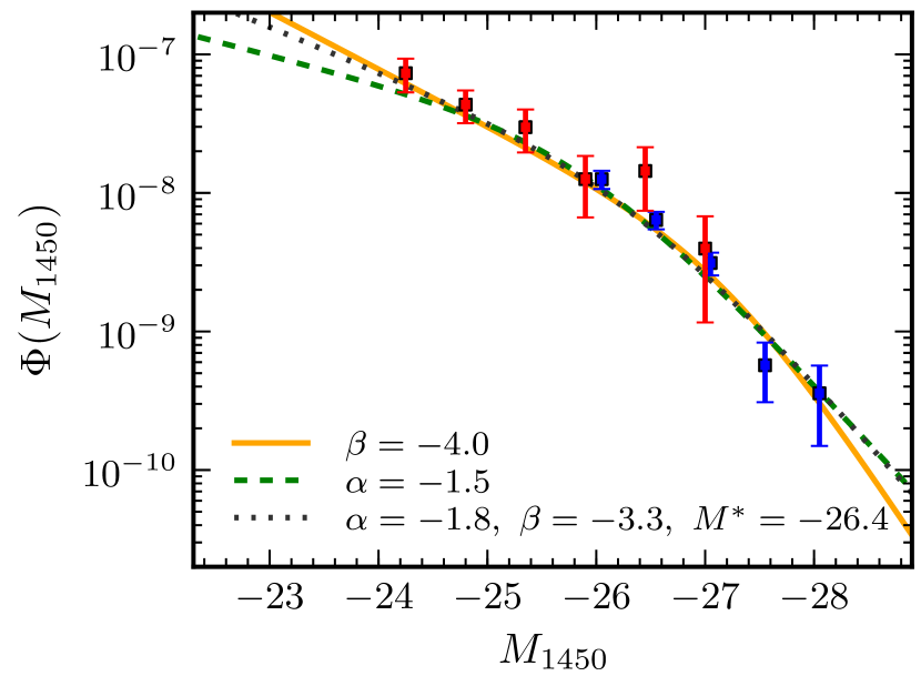
Table 3 and Figure 13 show the results of several model fits with various choices for the fixed parameters. Uncertainties derived by varying a single parameter and calculating the likelihood for the best-fit solution for the other parameters are included. First, we fix the bright end slope to . This value was chosen as it is approximately the slope derived from a single power-law fit to the brightest magnitude bins (§6.2). We choose to fix the bright end slope as we find that our fits prefer high values for the break luminosity; interestingly, this implies that the bright end slope is poorly constrained by our data (due to small numbers and limited luminosity range). This fit has a steep faint end slope and high break luminosity ( and ). We adopt these values as our best fit. Although the likelihoods can be improved by allowing even steeper values for , this tends to drive the break luminosity near the limit of our data, where both parameters have considerable freedom while fitting.
We further explore the parameter degeneracies by calculating the joint likelihood ranges for each of the power-law slopes and . Figure 14 shows probability contours for and , while allowing the other two parameters to vary. Figure 15 shows similar contours for and . Comparison of these two figures shows that is indeed more poorly constrained than .
Surveys of faint quasars typically find (Hunt et al. 2004; Richards et al. 2005; Siana et al. 2008; Croom et al. 2009), while observations at high redshift favor a steeper value of (Glikman et al. 2010; Ikeda et al. 2011; Masters et al. 2012), albeit with large uncertainties due to the difficulties of assembling large samples of faint quasars at high redshift. We find that a steeper value for the faint end slope is favored by our data, although lies within our contour.
Figure 15 shows that fits to our data similarly prefer steep values of . In fact, if we allow all of the parameters to be free, the maximum likelihood fitting tends to arbitrarily steep values for . We consider fits with to be effectively unconstrained, as this places the break luminosity at , where we have only a handful of quasars. We thus impose a ceiling on the likelihood based on a fit with , and calculate probability contours relative to this fit. Nonetheless, it is clear that is steep: at 95% confidence. Further observations of bright quasars at are needed to better constrain the bright-end slope at this redshift.
The strong constraints on the steepness of the bright end slope show that a flattening of the bright end slope at high redshift, as found by, e.g., Richards et al. (2006), is not in agreement with our data. This is likely due to the fact that Richards et al. (2006) fit a single power law slope to the SDSS data under the assumption that the break luminosity was well below their flux limit; we will discuss this further in the following section.
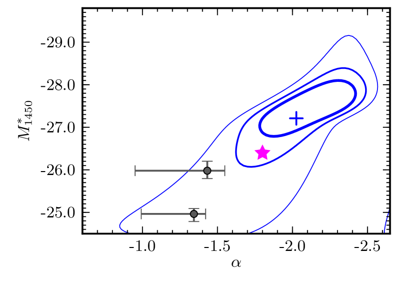
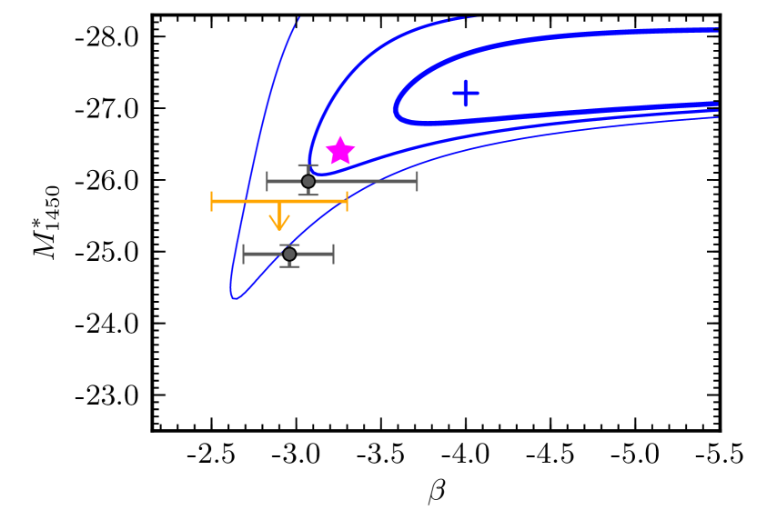
6.4. Evolution of the QLF
We provide some context for these fits by comparing to results at lower and higher redshift. Ross et al. (2012) recently presented a QLF measurement at from the BOSS DR9 quasar sample. Over this redshift range, the QLF is well-fit by a Luminosity Evolution and Density Evolution (LEDE) model, where the power law slopes have fixed values and the normalization and break luminosity evolve in a log-linear fashion. Specifically,
| (1) | |||||
| (2) |
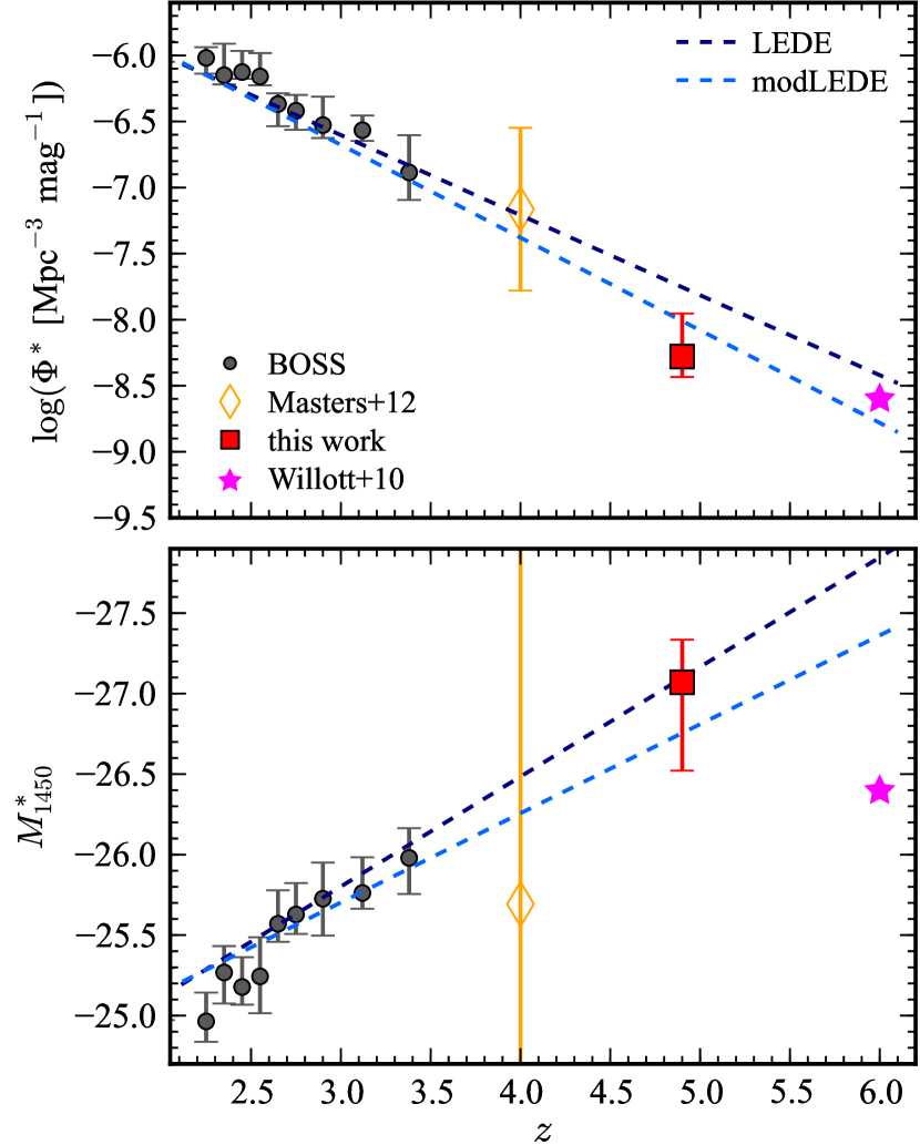
In equation 2, is the absolute -band magnitude at (Richards et al. 2006), corresponding to rest-frame Å and assuming a spectral index of (). The evolution in and given by this model is shown in Figure 16, extrapolated to higher redshift to compare with our data. While evolution in the power law slopes is not well constrained by the data, our slopes are reasonably consistent with the values obtained from the BOSS data, with some indication that the faint end slope steepens toward higher redshift (Figs. 14 and 15). However, the values for and do not agree with the simple extrapolation of the LEDE model from lower redshift. This can be clearly seen in Figure 17, which shows the LEDE prediction at significantly overestimates our measurements. We will discuss a modified form to the LEDE model that provides a better fit to the high redshift evolution in §6.6.
At higher redshift, we compare to the QLF measurement reported by Willott et al. (2010). The last row of Table 3 shows the results of a fit where all the parameters except have been fixed to the best-fit values from Willott et al. (2010) for a fixed faint end slope of (we use this value as it provides a better fit to our data than their fit). Figures 14 and 15 show that the , , and from the Willott et al. (2010) QLF lie near the contours from our constraints at ; however, the uncertainties on the Willott et al. (2010) values are not available and would likely eliminate any tension between the fitted values at and (see, e.g., their Figure 6 for the uncertainties on and for a fit with ). What is more clear is that the normalization is quite different: it is a factor of higher than predicted by evolving the Willott et al. (2010) model to using , as they adopted for their fit (they obtained , in contrast to the value of we obtain when fitting the shape of their QLF to our data). Figure 17 illustrates the discrepancy in the normalization from the evolved Willott et al. (2010) model; we will discuss this point further in § 6.6.
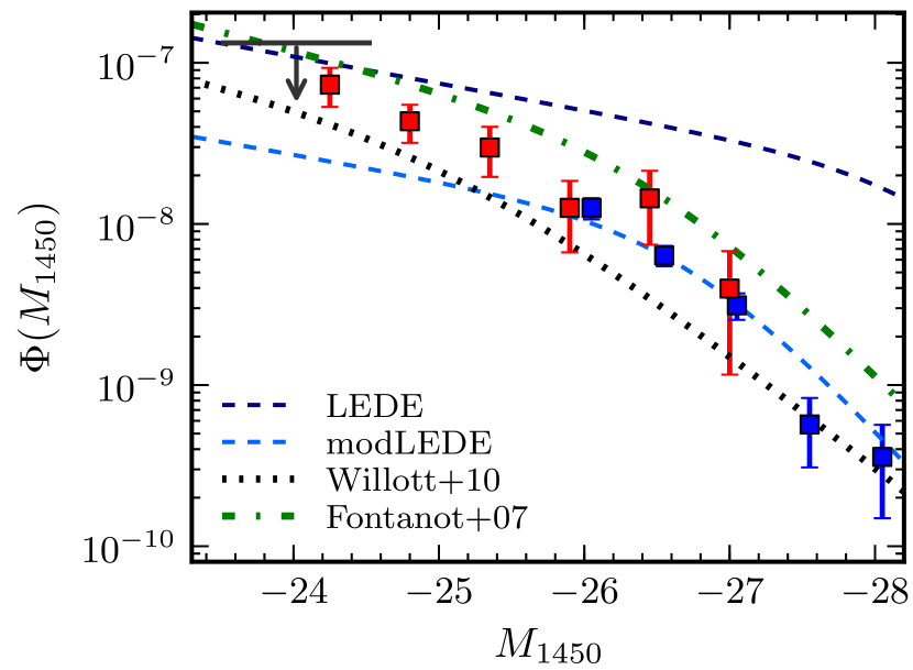
The empirical QLF model of Hopkins et al. (2007b, hereafter HRH07) combines observations in the optical, X-ray, and mid-infrared bands to construct a bolometric QLF from to . At high redshift the most constraining data in HRH07 comes from optical surveys, which have shown a flattening of the bright end slope at high redshift (Schmidt et al. 1995; Fan et al. 2001b; Richards et al. 2006). In the HRH07 model, the break luminosity increases with redshift until and then turns over, such that it is a factor of lower luminosity at than at . At , the HRH07 model predicts a quite low break luminosity () and a shallow bright end slope (). Figure 12 shows that the HRH07 model agrees with our data at , which is not surprising since at their fit is mainly to the Richards et al. (2006) data. The agreement at lower luminosities arises because the bright end slope from HRH07 roughly agrees with our faint end slope. At the bright end, we attribute the disagreement between our data and the HRH07 QLF to a steeper slope and a much brighter than predicted by their model. This demonstrates the substantial degeneracies in the QLF parameters, as the HRH07 values for and at would not even appear on Figure 16, even though the model itself provides a good fit to our data at . The key difference between our work and HRH07 (and by extension, Richards et al. 2006) is the increased survey area at the bright end, which is needed to extend above the break luminosity at this redshift and make the break in the luminosity function more evident.
Finally, we examine the QLF from Fontanot et al. (2007). This work combines bright quasars from SDSS DR3 with faint quasars from the Great Observatories Origins Deep Survey (GOODS; Dickinson et al. 2003) over the redshift range . Figure 17 compares their pure density evolution (PDE) model (#12 from their Table 3) to our data. We find that the Fontanot et al. (2007) model overestimates our QLF measurements at all luminosities. Ikeda et al. (2012) similarly found some tension between their constraint derived from observations of quasar candidates drawn from COSMOS (Scoville et al. 2007), and suggested this may be due to the completenesss correction applied by Fontanot et al. (2007). We show the Ikeda et al. (2012) upper limit in Figure 17.
In conclusion, we find evidence for a steepening of the faint end slope, and no evidence in favor of an evolution in the bright end slope, although obtaining strong constraints on the evolutionary forms of these parameters is difficult with existing data. On the other hand, we do see evidence for strong evolution in the break luminosity, as it brightens from at to at (Figure 16). This evolution has consequences for surveys where the faint limit is near the break luminosity, as single power law fits to such data would naturally find a flatter slope. The problem is evident in Figure 12, which shows that a single power law can describe the SDSS DR3 data from Richards et al. (2006), the full range of which is near the break luminosity. The possibility that high redshift fits to the bright end of the QLF may be biased by a higher break luminosity was put forward by Assef et al. (2011) and Shen & Kelly (2012). Based on our fits at and the greater dynamic range of our survey, we find this scenario to be plausible; i.e., the flattening of the bright end slope at high redshift reported previously (Schmidt et al. 1995; Fan et al. 2001b; Richards et al. 2006; Hopkins et al. 2007b) may be attributed instead to rapid evolution in the break luminosity.
6.5. Comparison to Theoretical Predictions
Figure 18 compares our data to various theoretical models for the QLF at . Shen (2009) provides a theoretical prediction for the evolution of the QLF in a cosmological framework by relating the growth of SMBHs to the hierarchical assembly of their host dark matter halos. In this model, quasar activity is triggered by major mergers of halos. Their fiducial model reproduces the observed QLF at , but underpredicts the observed QLF at higher redshifts. Indeed, their fiducial model lies below our data at (Figure 18). Shen (2009) also has a variant of this fiducial model that includes a faster redshift evolution in the normalization of the scaling relation between peak quasar luminosity and host halo mass, a redshift evolution in the scatter of this relation and an increase in the upper host halo mass above which quasar triggering is cut off exponentially in order to better fit the QLF at higher redshifts (see Sec. 4.4 of Shen 2009, for details). This alternative model provides a good fit to our data at the bright end, but overpredicts the number counts at the faint end.
Conroy & White (2012) introduce a model in which quasars are tied to galaxies in a straightforward manner through the relation, so that the evolution of the QLF is determined by the evolution of this relation. Their model includes two free parameters that are allowed to vary with redshift: the quasar duty cycle and the normalization of the relation. Conroy & White (2012) constrain these parameters from existing QLF measurements at . The high redshift constraints mainly come from the SDSS (Richards et al. 2006) and have limited dynamic range, leading to significant uncertainties in the prediction (represented by the gray shaded region in Figure 18, see also Fig. 3 in Conroy & White 2012). Overall, the Conroy & White (2012) model provides a good fit to the data.
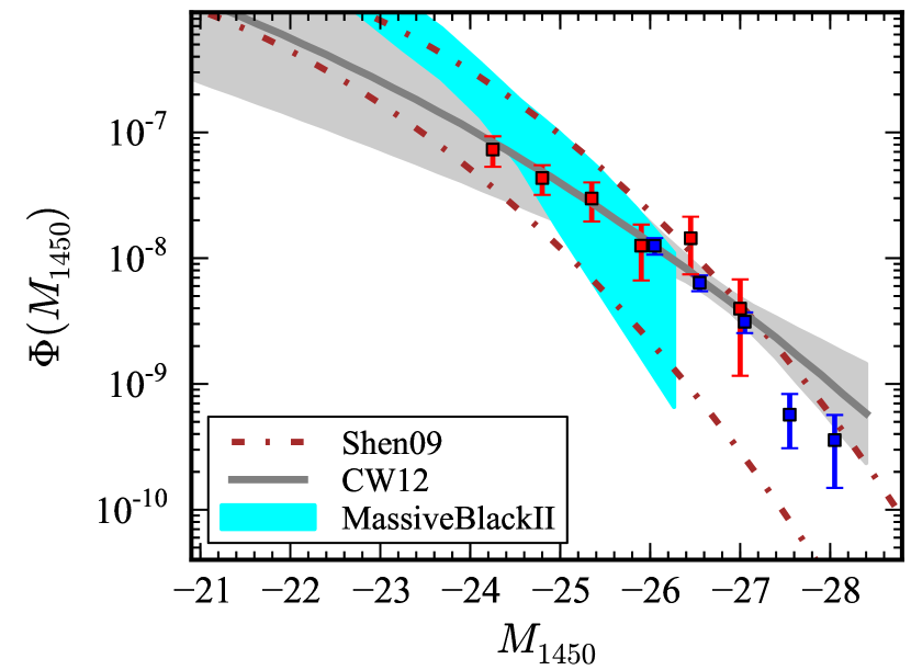
Degraf et al. (2010) present a QLF prediction based on hydrodynamic simulations that include radiative cooling, star formation, black holes, and feedback processes. This work has since been updated to a larger simulation volume, with 100 Mpc on a side and 2x17923 particles (MassiveBlackII; DeGraf et al, in prep.). At each timestep, the QLF is calculated from the active black holes, and the final QLF prediction is derived by time-averaging the individual measurements. This allows the bright end of the QLF to be estimated by catching the brief episodes of peak luminosity among the rare, massive black hole population. Figure 18 shows the prediction of this model in our redshift range, including an estimate for cosmic variance derived by comparing two simulation volumes (represented by the extent of the shaded region). This model generally agrees with our data near and just below the break luminosity. It appears to be somewhat steeper than the data at faint luminosities, though fainter measurements of the QLF from deeper optical data or at other wavelengths (e.g., X-rays) are needed to better constrain the model.
We remind the reader that our QLF only accounts for unobscured, Type I quasars. Our measurements are lower limits on the true density of actively accreting black holes, assuming some fraction are in an obscured (or even mildly extincted) growth phase. For example, comparison to X-ray surveys indicates that only % of quasars are unobscured at (Masters et al. 2012). Some inconsistency with theoretical models that do not distinguish between unobscured and obscured quasars is thus expected. Furthermore, a luminosity dependence for the obscured fraction (e.g., Ueda et al. 2003) could further bias comparisons of the data with theoretical models.
6.6. Spatial Density of Luminous Quasars
A rapid decline in the comoving number density of quasars at high redshift was observed three decades ago (Osmer 1982). Following Fan et al. (2001a), we quantify this evolution in terms of the spatial density of quasars above a minimum luminosity within a redshift window. The density is derived from the method, where for each quasar the volume within which it would have been observed within a survey is
where is again the selection function for the survey. From this equation, the total spatial density and its uncertainty are estimated by
where the sum is over all quasars more luminous than . This density is related to the luminosity function in that
| (3) |
where is the space density of quasars more luminous than . We choose to perform a sum over our data rather than an integration over the QLF as the latter requires extrapolation and model fitting. We calculate this quantity at , , and , combining data from SDSS, our work, and multiple surveys at . We choose a limit of as it corresponds to the lowest luminosity quasars in the SDSS sample at .
At we use the uniform quasar sample from the SDSS DR7 described in §6.1.1. This sample includes 311 quasars with , representing a factor of four increase in number over the SDSS DR3 results given in Richards et al. (2006). We adopt the selection function given in Table 1 of that work rather than recalculate it from our simulations, as the SDSS quasar target selection has a complicated dependence on the extent of the stellar locus in color space (Richards et al. 2002), which is captured by the Richards et al. (2006) selection function. At we use our combined sample from the SDSS DR7 and from Stripe 82 and the selection functions presented in section 6.1. Finally, at we use the sample compiled by Willott et al. (2010), consisting of quasars from the SDSS main (Fan et al. 2001a, 2003, 2004, 2006b), SDSS deep (Jiang et al. 2008, 2009), and CFHTQS (Willott et al. 2010). We derive selection functions for the three quasar surveys using our quasar simulations, extended to higher redshift. The derived selection functions from our models agree well with those shown in Figure 4 of Willott et al. (2010).
Figure 19 shows the evolution of the space density of luminous quasars () from to . Our measurement at shows a decline in the space density by a factor of 1.8 from . Fan et al. (2001b) fit an exponential decline to the space density at high redshifts, finding that with at , about a factor of three per unit redshift. Brusa et al. (2009) reported a similar value () using X-ray-selected quasars at (). Our results from to are in good agreement with these results; we measure a decline of per unit redshift ().
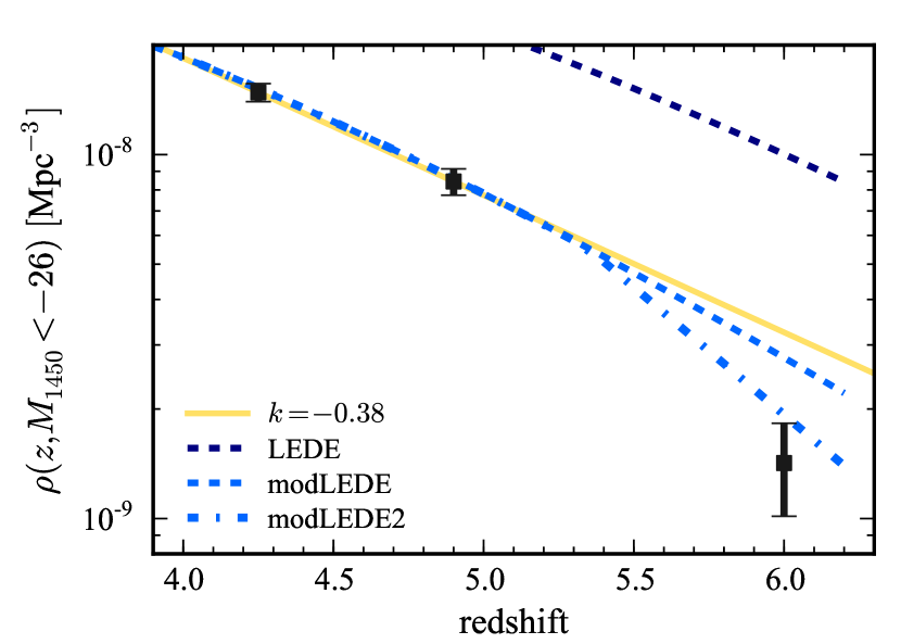
On the other hand, the evolution to is more pronounced: a factor of per unit redshift (), or roughly twice the rate measured at lower redshift (Figure 19). The departure of the measurement from the prediction based on the slope fit to the data is significant at the level. If we integrate deeper for the two high redshift bins, to a limit of , the decline is even stronger. We obtain and , corresponding to a factor of decline per unit redshift.
We check the consistency of our faint-end measurements by comparing to recent work at X-ray wavelengths with the Chandra-COSMOS survey (Civano et al. 2011), which is sensitive to moderate-luminosity () AGN at . In order to compare the two samples, we must integrate our double power law model to (adopting the relation from Young et al. 2010). Civano et al. (2011) identified three X-ray-selected Type I quasars in the redshift bin , which translates to an observed space density of . Integrating our best-fit model for the QLF over that redshift bin, we obtain . Thus our QLF agrees with the Civano et al. (2011) results to within the uncertainties, especially when considering that to make the comparison we must extrapolate our QLF in both luminosity and redshift. The X-ray data do not strongly constrain the evolution to due to the small area of the Chandra-COSMOS survey (from zero objects in Civano et al. 2011, the decline from to is per unit redshift).
We now relate the decline in the high-redshift quasar density to the evolutionary model for the QLF derived from the BOSS DR9 (Ross et al. 2012). In this LEDE model, declines by 0.6 dex per unit redshift, while brightens by 0.68 mag per unit redshift ( in equation 1 and in equation 2, respectively). Integrating this model (equation 3) shows that it significantly overpredicts the high redshift number densities we have derived (Figure 19). This result suggests that the steeper decline in the high-redshift number counts begins at , and is also consistent with Figure 16, which shows that the predicted by the LEDE model is higher than the data at , and is not well constrained at . We thus modify the LEDE model from BOSS by steepening the slope of the evolution to , and softening the slope of the evolution to . These modifications are within the uncertainties of the values derived from fitting BOSS data; Figure 19 shows that they bring the QLF model in agreement with the integral constraints from the data, but not the point. At , this modified evolutionary model predicts and . This provides a good match to the values we obtained when fixing the slopes to the BOSS values during the MLE fit, and (Table 3).
Finally, we consider further modifying the model for the evolution of . It is unlikely that continues to rise to very high luminosities; indeed, Figure 16 shows that the high-redshift fits for are somewhat below the LEDE prediction. We thus impose a maximum break luminosity of , which in the modified LEDE model is reached at . This choice causes a turnover in the high-redshift number densities that matches the data at (Figure 19). This model is somewhat arbitrary, but qualitatively, a model in which has a more rapid downward evolution at high redshift and brightens until and then levels off (or even turns over) provides a reasonable description of the high redshift data. A quasar with radiating at the Eddington luminosity corresponds to a black hole; it seems reasonable to suppose that while the break luminosity evolves strongly at high redshift, it would not greatly exceed this value.
6.7. Contribution of quasars to the ionizing background
The number of ionizing photons required to maintain hydrogen ionization as a function of redshift can be found by balancing the ionizing photon emissivity with the density of hydrogen and the rate of recombinations. The recombination rate depends on the clumping factor, . Madau et al. (1999) present an equation for the ionizing photon density that adopts a high value for the clumping factor (). More recent work suggests that the clumping factor is not so large; Meiksin (2005) argues that and McQuinn et al. (2011) use cosmological simulations that include the effects of Lyman-limit systems and find at . Similarly, both Shull et al. (2012a) and Finlator et al. (2012) prefer a lower clumping factor of at in their reionization models.
We calculate the ionizing photon output for each quasar by assuming a broken power-law SED with an index of at ultraviolet wavelengths (Telfer et al. 2002), a break at 1100Å, and an index of above the break111111We also tested the far-UV spectral slope from Shull et al. (2012b) with and found that it changes the results by only a few percent.. Rescaling the Madau et al. (1999) equation and updating to our cosmology, we estimate the number of photons required to maintain full ionization at to be . Integrating the best-fit QLF model (with ) to gives , or % of the number required (for the flatter faint-end slopes, the percentage lowers to %). For , quasars provide % of the photons required for hydrogen ionization, suggesting they may have played some role in maintaining ionization at . However, the steeper decline of luminous quasars from to further reduces the likelihood that quasars were an important source of ionizing photons during the reionization epoch. Indeed, even when assuming a steep faint-end slope (), Willott et al. (2010) find that quasars generate of the required ionizing photon background. This is also in good agreement with constraints from deep X-ray surveys (Barger et al. 2003; Fontanot et al. 2007) that limit the contribution from moderate luminosity AGN at .
7. Conclusions
This work builds on the legacy of SDSS Stripe 82 for high-redshift quasar studies. Fan et al. (2004) first used coadded photometry from epochs of Stripe 82 imaging to discover a single quasar with , fainter than the limit adopted for the single-epoch imaging. Subsequently, Jiang et al. (2008, 2009) created deep, coadded images from the epochs available at the completion of SDSS I/II to discover 11 quasars at to a limit of . In this work, we have utilized the bluer SDSS bands to conduct a survey of quasars, a redshift where current constraints on the QLF are relatively weak.
We define a sample of 92 candidates to a limit of using color selection criteria and with a well-defined selection function. From this sample, 73 objects have spectroscopic observations, and 71 are confirmed high redshift quasars. We then focus on the redshift range where our completeness is highest. Using a sample of 52 quasars from our work on Stripe 82 combined with 146 bright quasars from the SDSS DR7, we calculate the optical quasar luminosity function at .
We have fit a double power law model to our observational data at , and reach the following conclusions:
-
•
There is no clear evidence for evolution in the shape of the QLF from to . We find a steep bright-end slope (, Fig. 12) that roughly agrees with measurements at both lower (e.g., BOSS , Ross et al. 2012) and higher (, Willott et al. 2010; Jiang et al. 2009) redshifts. While the bright-end slope is not well determined due to small numbers, it is strongly constrained to be steep, with at 95% confidence; thus we do not confirm previous findings that flattens at high redshift (e.g., Richards et al. 2006). A relatively steep value for the faint end slope is favored () in agreement with other high redshift results.
-
•
We see the break in the luminosity function in our data, finding that for (Fig. 15 Table 3). The strong covariances between the power law slopes and the break luminosity lead to significant uncertainties in these quantities, but the best fit value for the break luminosity is signficantly higher than at , where the BOSS results find .
-
•
The decline in the space density of luminous quasars at high redshift is greater than indicated by previous surveys. We find that while the decline in the integrated space density of quasars with from to is about a factor of three per unit redshift, in agreement with previous results, the decline to is nearly a factor of two greater (Fig. 19). This suggests a much more rapid dropoff in luminous quasar activity at the highest redshifts currently probed by observations.
-
•
By comparing to a simple LEDE model for the redshift evolution of BOSS quasars, we find that in addition to the steeper decline in number density, there is also an indication that the brightening of the break luminosity with redshift does not continue indefinitely. A toy model in which the evolution of is somewhat steeper than from a simple extrapolation from the BOSS data, and in which the break luminosity evolves somewhat more slowly and peaks at , provides a good match to the high redshift data.
-
•
Our model for the QLF at predicts that quasars contribute % of the ionizing photons required to maintain hydrogen ionization at this redshift, with the uncertainty dominated by our lack of understanding of the clumping factor.
The strong evolution in the high redshift quasar number density we have found has implications for quasar surveys at even higher redshifts. Early forecasts for UKIDSS anticipated roughly 10 quasars from the survey (Warren & Hewett 2002), much greater than the one found to date (Mortlock et al. 2011) from over half the survey area. Using a redshift evolution of (Fan et al. 2001b), extrapolation of our QLF predicts that there are quasars at in the UKIDSS DR8plus release to a limit of (see Fig. 7 of Mortlock et al. 2012). Using the same evolutionary factor, the QLF from Willott et al. (2010) predicts quasars in this redshift range. Based on our results, these estimates should be revised downward to and , respectively. The lower yield from UKIDSS is at least consistent with the steeper evolution at we have found; further, the decline may continue to steepen at , resulting in even smaller numbers of luminous quasars.
Significant progress has been made over the last decade in measuring the evolution of the high redshift quasar population. Nonetheless, the observations are not yet strongly constraining of models that make, for example, different predictions for the evolution of the power law slopes. Ongoing high redshift quasar surveys will improve these constraints. We are currently extending our work to fainter luminosities at using deeper optical imaging data, obtaining improved measurements of the faint end slope and break luminosity. We will also use Stripe 82 data to measure the QLF at over a wide range of luminosities. Finally, Pan-STARRS (Kaiser et al. 2002) is obtaining shallow optical and near-infrared imaging, including the -band, over an area of sky over that is more than twice that of the SDSS. To date, one quasar has been discovered from this survey (Morganson et al. 2012); future work should reduce the uncertainty on the bright end of the QLF at and better constrain the strong evolution we have measured from existing data.
8. Acknowledgements
The authors thank the staffs of the MMT and Magellan telescopes, particularly the recently retired John McAfee, for enabling many of the observations presented here. IDM, LJ and XF acknowledge support from a David and Lucile Packard Fellowship, and NSF Grants AST 08-06861 and AST 11-07682. L.J. acknowledges support from NASA through Hubble Fellowship grant HST-HF-51291.01 awarded by the STScI.
Funding for SDSS-III has been provided by the Alfred P. Sloan Foundation, the Participating Institutions, the National Science Foundation, and the U.S. Department of Energy Office of Science. The SDSS-III web site is http://www.sdss3.org/.
SDSS-III is managed by the Astrophysical Research Consortium for the Participating Institutions of the SDSS-III Collaboration including the University of Arizona, the Brazilian Participation Group, Brookhaven National Laboratory, University of Cambridge, Carnegie Mellon University, University of Florida, the French Participation Group, the German Participation Group, Harvard University, the Instituto de Astrofisica de Canarias, the Michigan State/Notre Dame/JINA Participation Group, Johns Hopkins University, Lawrence Berkeley National Laboratory, Max Planck Institute for Astrophysics, Max Planck Institute for Extraterrestrial Physics, New Mexico State University, New York University, Ohio State University, Pennsylvania State University, University of Portsmouth, Princeton University, the Spanish Participation Group, University of Tokyo, University of Utah, Vanderbilt University, University of Virginia, University of Washington, and Yale University.
Facilities: MMT (Red Channel spectrograph, SWIRC), Magellan:Clay (MAGE), SDSS
References
- Abazajian et al. (2009) Abazajian, K. N., Adelman-McCarthy, J. K., Agüeros, M. A., et al. 2009, ApJS, 182, 543
- Ahn et al. (2012) Ahn, C. P., Alexandroff, R., Allende Prieto, C., et al. 2012, ApJS, 203, 21
- Aihara et al. (2011) Aihara, H., Allende Prieto, C., An, D., et al. 2011, ApJS, 193, 29
- Annis et al. (2011) Annis, J., Soares-Santos, M., Strauss, M. A., et al. 2011, ArXiv e-prints, 1111.6619
- Assef et al. (2011) Assef, R. J., Kochanek, C. S., Ashby, M. L. N., et al. 2011, ApJ, 728, 56
- Avni & Bahcall (1980) Avni, Y., & Bahcall, J. N. 1980, ApJ, 235, 694
- Baldwin (1977) Baldwin, J. A. 1977, ApJ, 214, 679
- Barger et al. (2003) Barger, A. J., Cowie, L. L., Capak, P., et al. 2003, ApJ, 584, L61
- Becker et al. (1995) Becker, R. H., White, R. L., & Helfand, D. J. 1995, ApJ, 450, 559
- Bertin & Arnouts (1996) Bertin, E., & Arnouts, S. 1996, A&AS, 117, 393
- Bertin et al. (2002) Bertin, E., Mellier, Y., Radovich, M., et al. 2002, in Astronomical Society of the Pacific Conference Series, Vol. 281, Astronomical Data Analysis Software and Systems XI, ed. D. A. Bohlender, D. Durand, & T. H. Handley, 228
- Bochanski et al. (2009) Bochanski, J. J., Hennawi, J. F., Simcoe, R. A., et al. 2009, PASP, 121, 1409
- Bolton et al. (2012) Bolton, A. S., Schlegel, D. J., Aubourg, E., et al. 2012, ApJ
- Bolton et al. (2009) Bolton, J. S., Oh, S. P., & Furlanetto, S. R. 2009, MNRAS, 395, 736
- Bovy et al. (2011) Bovy, J., Hennawi, J. F., Hogg, D. W., et al. 2011, ApJ, 729, 141
- Boyle et al. (2000) Boyle, B. J., Shanks, T., Croom, S. M., et al. 2000, MNRAS, 317, 1014
- Boyle et al. (1988) Boyle, B. J., Shanks, T., & Peterson, B. A. 1988, MNRAS, 235, 935
- Brotherton et al. (2001) Brotherton, M. S., Tran, H. D., Becker, R. H., et al. 2001, ApJ, 546, 775
- Brown et al. (2008) Brown, W. R., McLeod, B. A., Geary, J. C., & Bowsher, E. C. 2008, in Society of Photo-Optical Instrumentation Engineers (SPIE) Conference Series, Vol. 7014, Society of Photo-Optical Instrumentation Engineers (SPIE) Conference Series
- Brusa et al. (2009) Brusa, M., Comastri, A., Gilli, R., et al. 2009, ApJ, 693, 8
- Carlberg (1990) Carlberg, R. G. 1990, ApJ, 350, 505
- Casali et al. (2007) Casali, M., Adamson, A., Alves de Oliveira, C., et al. 2007, A & A, 467, 777
- Cattaneo et al. (1999) Cattaneo, A., Haehnelt, M. G., & Rees, M. J. 1999, MNRAS, 308, 77
- Chiu et al. (2005) Chiu, K., Zheng, W., Schneider, D. P., et al. 2005, AJ, 130, 13
- Civano et al. (2011) Civano, F., Brusa, M., Comastri, A., et al. 2011, ApJ, 741, 91
- Conroy & White (2012) Conroy, C., & White, M. 2012, ArXiv e-prints, 1208.3198
- Cowie et al. (2003) Cowie, L. L., Barger, A. J., Bautz, M. W., Brandt, W. N., & Garmire, G. P. 2003, ApJ, 584, L57
- Croom et al. (2009) Croom, S. M., Richards, G. T., Shanks, T., et al. 2009, MNRAS, 399, 1755
- Dawson et al. (2012) Dawson, K. S., Schlegel, D. J., Ahn, C. P., et al. 2012, ApJ
- Degraf et al. (2010) Degraf, C., Di Matteo, T., & Springel, V. 2010, MNRAS, 402, 1927
- Di Matteo et al. (2012) Di Matteo, T., Khandai, N., DeGraf, C., et al. 2012, ApJ, 745, L29
- Di Matteo et al. (2005) Di Matteo, T., Springel, V., & Hernquist, L. 2005, Nature, 433, 604
- Diamond-Stanic et al. (2009) Diamond-Stanic, A. M., Fan, X., Brandt, W. N., et al. 2009, AJ, 699, 782
- Dickinson et al. (2003) Dickinson, M., Giavalisco, M., & GOODS Team. 2003, in The Mass of Galaxies at Low and High Redshift, ed. R. Bender & A. Renzini, 324, arXiv:astro-ph/0204213
- Dijkstra et al. (2004) Dijkstra, M., Haiman, Z., & Loeb, A. 2004, ApJ, 613, 646
- Eisenstein et al. (2011) Eisenstein, D. J., Weinberg, D. H., Agol, E., et al. 2011, ApJ, 142, 72
- Fan (1999) Fan, X. 1999, AJ, 117, 2528
- Fan et al. (2004) Fan, X., Hennawi, J. F., Richards, G. T., et al. 2004, AJ, 128, 515
- Fan et al. (2001a) Fan, X., Narayanan, V. K., Lupton, R. H., et al. 2001a, AJ, 122, 2833
- Fan et al. (2006a) Fan, X., Strauss, M. A., Becker, R. H., et al. 2006a, AJ, 132, 117
- Fan et al. (2006b) Fan, X., Strauss, M. A., Richards, G. T., et al. 2006b, AJ, 131, 1203
- Fan et al. (1999) Fan, X., Strauss, M. A., Schneider, D. P., et al. 1999, AJ, 118, 1
- Fan et al. (2001b) ——. 2001b, AJ, 121, 54
- Fan et al. (2003) ——. 2003, AJ, 125, 1649
- Finlator et al. (2012) Finlator, K., Oh, S. P., Özel, F., & Davé, R. 2012, MNRAS, 427, 2464
- Fontanot et al. (2007) Fontanot, F., Cristiani, S., Monaco, P., et al. 2007, A&A, 461, 39, arXiv:astro-ph/0608664
- Frieman et al. (2007) Frieman, J. A., Bassett, B., Becker, A., et al. 2007, AJ, 135, 338
- Fukugita et al. (1996) Fukugita, M., Ichikawa, T., Gunn, J. E., et al. 1996, AJ, 111, 1748
- Gaskell (1982) Gaskell, C. M. 1982, ApJ, 263, 79
- Glikman et al. (2010) Glikman, E., Bogosavljević, M., Djorgovski, S. G., et al. 2010, ApJ, 710, 1498
- Glikman et al. (2011) Glikman, E., Djorgovski, S. G., Stern, D., et al. 2011, ApJL, 728, L26
- Gunn et al. (1998) Gunn, J. E., Carr, M., Rockosi, C., et al. 1998, AJ, 116, 3040
- Gunn et al. (2006) Gunn, J. E., Siegmund, W. A., Mannery, E. J., et al. 2006, AJ, 131, 2332
- Haiman & Loeb (1998) Haiman, Z., & Loeb, A. 1998, ApJ, 503, 505
- Hambly et al. (2008) Hambly, N. C., Collins, R. S., Cross, N. J. G., et al. 2008, MNRAS, 384, 637
- Hasinger et al. (2005) Hasinger, G., Miyaji, T., & Schmidt, M. 2005, A & A, 441, 417
- Hernquist (1989) Hernquist, L. 1989, Nature, 340, 687
- Hewett et al. (2006) Hewett, P. C., Warren, S. J., Leggett, S. K., & Hodgkin, S. T. 2006, MNRAS, 367, 454
- Hodge et al. (2011) Hodge, J. A., Becker, R. H., White, R. L., Richards, G. T., & Zeimann, G. R. 2011, AJ, 142, 3
- Hodgkin et al. (2009) Hodgkin, S. T., Irwin, M. J., Hewett, P. C., & Warren, S. J. 2009, MNRAS, 394, 675
- Hogg et al. (2001) Hogg, D. W., Finkbeiner, D. P., Schlegel, D. J., & Gunn, J. E. 2001, AJ, 122, 2129
- Hopkins et al. (2005) Hopkins, P. F., Hernquist, L., Cox, T. J., et al. 2005, ApJ, 630, 716
- Hopkins et al. (2006) ——. 2006, ApJS, 163, 1
- Hopkins et al. (2007a) Hopkins, P. F., Lidz, A., Hernquist, L., et al. 2007a, ApJ, 662, 110
- Hopkins et al. (2007b) Hopkins, P. F., Richards, G. T., & Hernquist, L. 2007b, ApJ, 654, 731
- Huff et al. (2011) Huff, E. M., Hirata, C. M., Mandelbaum, R., et al. 2011, ArXiv e-prints, 1111.6958
- Hunt et al. (2004) Hunt, M. P., Steidel, C. C., Adelberger, K. L., & Shapley, A. E. 2004, ApJ, 605, 625
- Ikeda et al. (2011) Ikeda, H., Nagao, T., Matsuoka, K., et al. 2011, ApJL, 728, L25
- Ikeda et al. (2012) Ikeda, H., Nagao, T., Matsuoka, K., et al. 2012, ApJ, 756, 160, 1207.1515
- Ivezić et al. (2004) Ivezić, Ž., Lupton, R. H., Schlegel, D., et al. 2004, Astronomische Nachrichten, 325, 583
- Jiang et al. (2008) Jiang, L., Fan, X., Annis, J., et al. 2008, AJ, 135, 1057
- Jiang et al. (2009) Jiang, L., Fan, X., Bian, F., et al. 2009, AJ, 138, 305
- Jiang et al. (2006) Jiang, L., Fan, X., Hines, D. C., et al. 2006, AJ, 132, 2127
- Kaiser et al. (2002) Kaiser, N., Aussel, H., Burke, B. E., et al. 2002, in Society of Photo-Optical Instrumentation Engineers (SPIE) Conference Series, Vol. 4836, Society of Photo-Optical Instrumentation Engineers (SPIE) Conference Series, ed. J. A. Tyson & S. Wolff, 154–164
- Kauffmann & Haehnelt (2000) Kauffmann, G., & Haehnelt, M. 2000, MNRAS, 311, 576
- Kelly et al. (2008) Kelly, B. C., Fan, X., & Vestergaard, M. 2008, ApJ, 682, 874
- Kirkpatrick et al. (2011) Kirkpatrick, J. A., Schlegel, D. J., Ross, N. P., et al. 2011, ApJ, 743, 125
- Komatsu et al. (2009) Komatsu, E., Dunkley, J., Nolta, M. R., et al. 2009, ApJS, 180, 330
- Koo & Kron (1988) Koo, D. C., & Kron, R. G. 1988, ApJ, 325, 92
- Kuhn et al. (2001) Kuhn, O., Elvis, M., Bechtold, J., & Elston, R. 2001, ApJS, 136, 225
- Lampton et al. (1976) Lampton, M., Margon, B., & Bowyer, S. 1976, ApJ, 208, 177
- Lawrence et al. (2007) Lawrence, A., Warren, S. J., Almaini, O., et al. 2007, MNRAS, 379, 1599
- Lupton et al. (1999) Lupton, R. H., Gunn, J. E., & Szalay, A. S. 1999, AJ, 118, 1406
- Madau et al. (1999) Madau, P., Haardt, F., & Rees, M. J. 1999, ApJ, 514, 648
- Marshall et al. (1983) Marshall, H. L., Tananbaum, H., Avni, Y., & Zamorani, G. 1983, ApJ, 269, 35
- Marshall et al. (2008) Marshall, J. L., Burles, S., Thompson, I. B., et al. 2008, in Ground-based and Airborne Instrumentation for Astronomy II (SPIE), 701454–701454–10
- Masters et al. (2012) Masters, D., Capak, P., Salvato, M., et al. 2012, ApJ, 755, 169
- McDonald & Eisenstein (2007) McDonald, P., & Eisenstein, D. 2007, PhRevD, 76, 063009
- McQuinn (2012) McQuinn, M. 2012, MNRAS, 426, 1349
- McQuinn et al. (2011) McQuinn, M., Oh, S. P., & Faucher-Giguère, C.-A. 2011, ApJ, 743, 82
- Meiksin (2005) Meiksin, A. 2005, MNRAS, 356, 596
- Miralda-Escudé et al. (2000) Miralda-Escudé, J., Haehnelt, M., & Rees, M. J. 2000, ApJ, 530, 1
- Morganson et al. (2012) Morganson, E., De Rosa, G., Decarli, R., et al. 2012, AJ, 143, 142
- Mortlock et al. (2012) Mortlock, D. J., Patel, M., Warren, S. J., et al. 2012, MNRAS, 419, 390
- Mortlock et al. (2011) Mortlock, D. J., Warren, S. J., Venemans, B. P., et al. 2011, Nature, 474, 616
- Oke & Gunn (1983) Oke, J. B., & Gunn, J. E. 1983, AJ, 266, 713
- Osmer (1982) Osmer, P. S. 1982, ApJ, 253, 28
- Padmanabhan et al. (2008) Padmanabhan, N., Schlegel, D. J., Finkbeiner, D. P., et al. 2008, AJ, 674, 1217
- Page & Carrera (2000) Page, M. J., & Carrera, F. J. 2000, MNRAS, 311, 433
- Palanque-Delabrouille et al. (2012) Palanque-Delabrouille, N., Magneville, C., Yeche, C., et al. 2012, ArXiv e-prints, 1209.3968
- Palanque-Delabrouille et al. (2011) Palanque-Delabrouille, N., Yeche, C., Myers, A. D., et al. 2011, A & A, 530, 122
- Pâris et al. (2012) Pâris, I., Petitjean, P., Aubourg, É., et al. 2012, A & A, 548, 66
- Pei (1995) Pei, Y. C. 1995, ApJ, 438, 623
- Reichard et al. (2003) Reichard, T. A., Richards, G. T., Schneider, D. P., et al. 2003, AJ, 125, 1711
- Richards et al. (2005) Richards, G. T., Croom, S. M., Anderson, S. F., et al. 2005, MNRAS, 360, 839
- Richards et al. (2002) Richards, G. T., Fan, X., Newberg, H. J., et al. 2002, AJ, 123, 2945
- Richards et al. (2001) Richards, G. T., Fan, X., Schneider, D. P., et al. 2001, AJ, 121, 2308
- Richards et al. (2011) Richards, G. T., Kruczek, N. E., Gallagher, S. C., et al. 2011, AJ, 141, 167
- Richards et al. (2006) Richards, G. T., Strauss, M. A., Fan, X., et al. 2006, AJ, 131, 2766
- Ross et al. (2012) Ross, N. P., McGreer, I. D., White, M., et al. 2012, ArXiv e-prints, 1210.6389
- Ross et al. (2012) Ross, N. P., Myers, A. D., Sheldon, E. S., et al. 2012, ApJS, 199, 3
- Rousselot et al. (2000) Rousselot, P., Lidman, C., Cuby, J.-G., Moreels, G., & Monnet, G. 2000, A & A, 354, 1134
- Salpeter (1964) Salpeter, E. E. 1964, ApJ, 140, 796
- Scannapieco et al. (2005) Scannapieco, E., Silk, J., & Bouwens, R. 2005, ApJ, 635, L13
- Schlegel et al. (1998) Schlegel, D. J., Finkbeiner, D. P., & Davis, M. 1998, AJ, 500, 525
- Schmidt (1968) Schmidt, M. 1968, AJ, 151, 393
- Schmidt et al. (1995) Schmidt, M., Schneider, D. P., & Gunn, J. E. 1995, AJ, 110, 68
- Schneider et al. (2010) Schneider, D. P., Richards, G. T., Hall, P. B., et al. 2010, AJ, 139, 2360
- Schneider et al. (1991) Schneider, D. P., Schmidt, M., & Gunn, J. E. 1991, AJ, 102, 837
- Scoville et al. (2007) Scoville, N., Aussel, H., Brusa, M., et al. 2007, ApJS, 172, 1, arXiv:astro-ph/0612305
- Shen (2009) Shen, Y. 2009, ApJ, 704, 89
- Shen & Kelly (2012) Shen, Y., & Kelly, B. C. 2012, ApJ, 746, 169
- Shen et al. (2007) Shen, Y., Strauss, M. A., Oguri, M., et al. 2007, AJ, 133, 2222
- Shull et al. (2012a) Shull, J. M., Harness, A., Trenti, M., & Smith, B. D. 2012a, ApJ, 747, 100
- Shull et al. (2012b) Shull, J. M., Stevans, M., & Danforth, C. W. 2012b, ApJ, 752, 162
- Siana et al. (2008) Siana, B., Polletta, M. d. C., Smith, H. E., et al. 2008, ApJ, 675, 49
- Smee et al. (2012) Smee, S., Gunn, J. E., Uomoto, A., et al. 2012, ArXiv e-prints, 1208.2233
- Songaila (2004) Songaila, A. 2004, AJ, 127, 2598
- Songaila & Cowie (2010) Songaila, A., & Cowie, L. L. 2010, ApJ, 721, 1448
- Stoughton et al. (2002) Stoughton, C., Lupton, R. H., Bernardi, M., et al. 2002, AJ, 123, 485
- Telfer et al. (2002) Telfer, R. C., Zheng, W., Kriss, G. A., & Davidsen, A. F. 2002, ApJ, 565, 773
- Ueda et al. (2003) Ueda, Y., Akiyama, M., Ohta, K., & Miyaji, T. 2003, AJ, 598, 886
- van Dokkum (2001) van Dokkum, P. G. 2001, PASP, 113, 1420, arXiv:astro-ph/0108003
- Vanden Berk et al. (2005) Vanden Berk, D. E., Schneider, D. P., Richards, G. T., et al. 2005, AJ, 129, 2047
- Vestergaard & Wilkes (2001) Vestergaard, M., & Wilkes, B. J. 2001, ApJS, 134, 1
- Volonteri (2010) Volonteri, M. 2010, The Astronomy and Astrophysics Review, 18, 279
- Warren & Hewett (2002) Warren, S., & Hewett, P. 2002, in Astronomical Society of the Pacific Conference Series, Vol. 283, A New Era in Cosmology, ed. N. Metcalfe & T. Shanks, 369, arXiv:astro-ph/0201216
- Warren et al. (1994) Warren, S. J., Hewett, P. C., & Osmer, P. S. 1994, ApJ, 421, 412
- Weymann et al. (1991) Weymann, R. J., Morris, S. L., Foltz, C. B., & Hewett, P. C. 1991, ApJ, 373, 23
- Willott et al. (2005) Willott, C. J., Delfosse, X., Forveille, T., Delorme, P., & Gwyn, S. D. J. 2005, ApJ, 633, 630
- Willott et al. (2010) Willott, C. J., Delorme, P., Reylé, C., et al. 2010, AJ, 139, 906
- Worseck & Prochaska (2011) Worseck, G., & Prochaska, J. X. 2011, ApJ, 728, 23
- Wyithe & Loeb (2003) Wyithe, J. S. B., & Loeb, A. 2003, ApJ, 595, 614
- Yip et al. (2004) Yip, C. W., Connolly, A. J., Vanden Berk, D. E., et al. 2004, AJ, 128, 2603
- York et al. (2000) York, D. G., Adelman, J., Anderson Jr, J. E., et al. 2000, AJ, 120, 1579
- Young et al. (2010) Young, M., Elvis, M., & Risaliti, G. 2010, ApJ, 708, 1388
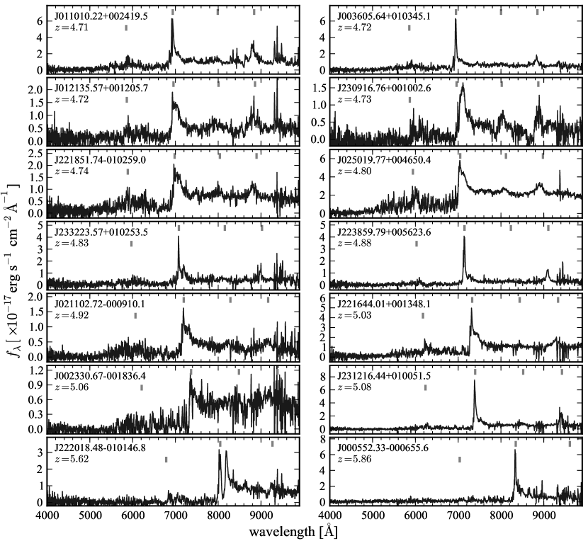
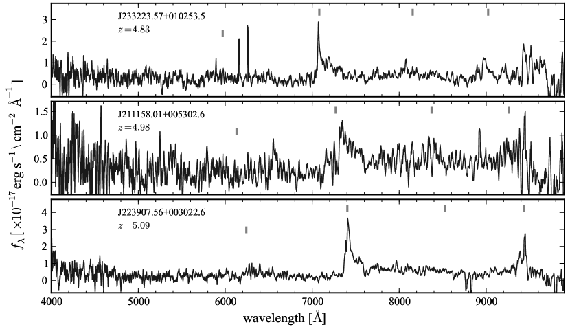
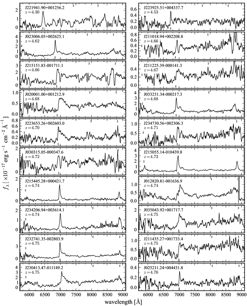
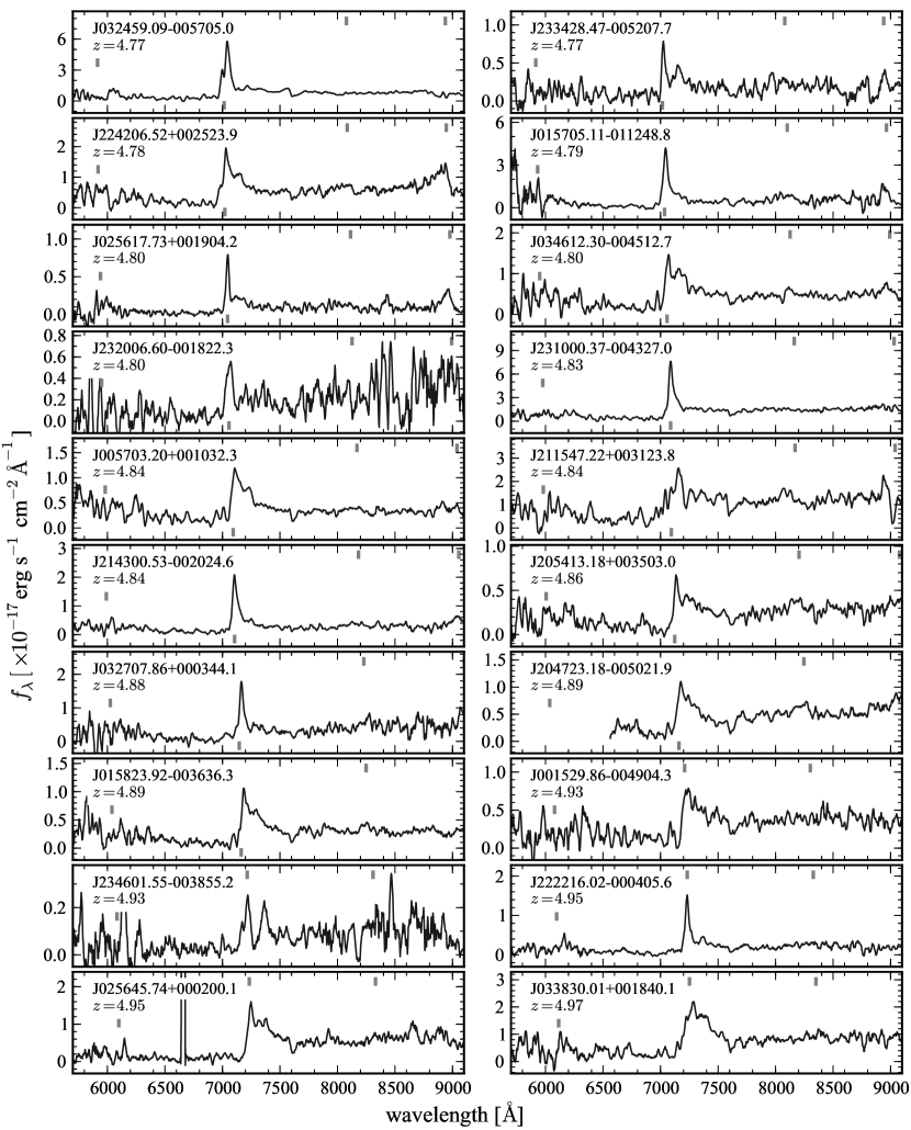
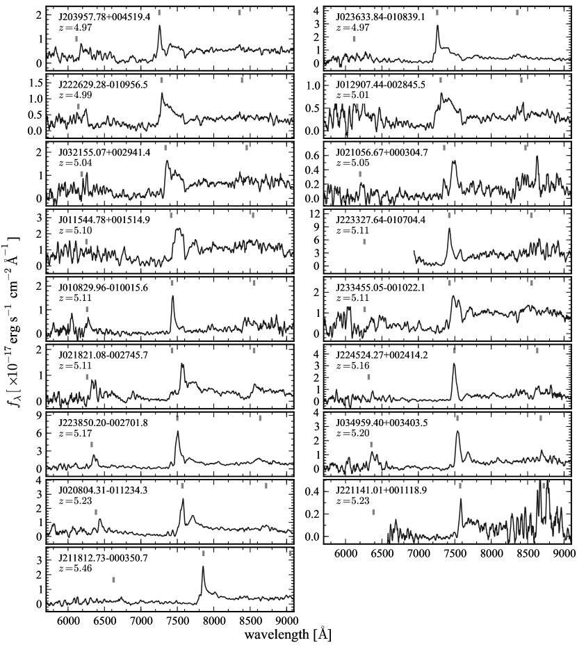
| RA (J2000) | Dec (J2000) | aaThe selection probability of spectroscopically confirming this object, including all sources of incompleteness (see §6.1.2). A value of indicates an object not included in the uniform sample. | NotesbbSpectroscopic identifications from MMT/Magellan show the UT date of the observation; those from BOSS give the plate-MJD-fiber of the observation. | |||||||
|---|---|---|---|---|---|---|---|---|---|---|
| 20:39:57.78 | +00:45:19.4 | -24.42 | 4.97 | 0.46 | 20120528 | |||||
| 20:47:23.18 | -00:50:21.9 | -24.79 | 4.89 | -1 | 20110624 | |||||
| 20:54:13.18 | +00:35:03.0 | -24.50 | 4.86 | 0.74 | 20120528 | |||||
| 21:10:18.94 | +00:22:08.8 | -24.63 | 4.66 | -1 | 20110623 | |||||
| 21:11:58.01 | +00:53:02.6 | -25.29 | 4.98 | -1 | 20110611 | |||||
| 21:12:25.39 | -00:01:41.3 | -24.99 | 4.67 | -1 | 20110623 | |||||
| 21:14:35.27 | +00:17:33.4 | cc magnitude from SWIRC. | -24.89 | 4.75 | 0.84 | 20111002 | ||||
| 21:15:47.22 | +00:31:23.8 | -25.27 | 4.84 | 0.77 | 20120528 | |||||
| 21:18:12.73 | -00:03:50.7 | -25.64 | 5.46 | -1 | 20120528 | |||||
| 21:30:08.93 | +00:26:09.8 | -26.08 | 4.95 | 0.62 | DR7 | |||||
| 21:43:00.53 | -00:20:24.6 | -24.11 | 4.84 | 0.28 | 20120527 | |||||
| 21:50:55.14 | -01:04:39.8 | -24.45 | 4.73 | 0.79 | 20120527 | |||||
| 21:51:51.83 | -00:17:11.1 | cc magnitude from SWIRC. | -25.23 | 4.66 | -1 | 20111002 | ||||
| 21:54:45.28 | +00:04:21.7 | -24.05 | 4.74 | 0.41 | 20120528 | |||||
| 22:00:08.66 | +00:17:44.9 | -27.11 | 4.82 | 0.88 | DR7 | |||||
| 22:11:41.01 | +00:11:18.9 | -24.84 | 5.23 | -1 | 20110624 | |||||
| 22:12:51.50 | -00:42:30.7 | -26.43 | 4.95 | 0.61 | DR7 | |||||
| 22:16:44.01 | +00:13:48.1 | -26.07 | 5.03 | 0.40 | 4200-55499-975 | |||||
| 22:18:51.74 | -01:02:59.0 | -25.23 | 4.74 | 0.84 | 4201-55443-370 | |||||
| 22:19:41.90 | +00:12:56.2 | cc magnitude from SWIRC. | -24.37 | 4.30 | -1 | 20111002 | ||||
| 22:20:18.48 | -01:01:46.8 | -25.83 | 5.62 | -1 | 4201-55443-246 | |||||
| 22:20:50.80 | +00:19:59.1 | -25.95 | 4.72 | 0.90 | DR7 | |||||
| 22:22:16.02 | -00:04:05.6 | -24.29 | 4.95 | 0.32 | 20120528 | |||||
| 22:25:09.19 | -00:14:06.8 | -27.28 | 4.89 | 0.72 | DR7 | |||||
| 22:26:29.28 | -01:09:56.5 | -24.57 | 4.99 | 0.55 | 20120527 | |||||
| 22:33:27.64 | -01:07:04.4 | -24.97 | 5.11 | -1 | 20110624 | |||||
| 22:36:53.26 | +00:26:03.0 | -23.92 | 4.70 | -1 | 20120528 | |||||
| 22:38:50.20 | -00:27:01.8 | cc magnitude from SWIRC. | -25.13 | 5.17 | -1 | 20111002 | ||||
| 22:38:59.79 | +00:56:23.6 | -25.23 | 4.88 | -1 | 4204-55470-710 | |||||
| 22:39:07.56 | +00:30:22.6 | -25.23 | 5.09 | 0.33 | 20110613 | |||||
| 22:39:25.51 | +00:43:37.7 | -24.11 | 4.53 | -1 | 20120528 | |||||
| 22:42:06.52 | +00:25:23.9 | -24.14 | 4.78 | 0.52 | 20111002 | |||||
| 22:45:24.27 | +00:24:14.2 | cc magnitude from SWIRC. | -24.88 | 5.16 | -1 | 20111002 | ||||
| 23:04:13.47 | -01:11:49.2 | -24.75 | 4.75 | 0.84 | 20111002 | |||||
| 23:09:16.76 | +00:10:02.6 | -25.08 | 4.73 | 0.83 | 4208-55476-896 | |||||
| 23:10:00.37 | -00:43:27.0 | -25.21 | 4.83 | 0.77 | 20111002 | |||||
| 23:12:16.44 | +01:00:51.5 | -25.61 | 5.08 | -1 | 4209-55478-714 | |||||
| 23:20:06.60 | -00:18:22.3 | -24.44 | 4.80 | 0.77 | 20111002 | |||||
| 23:27:41.35 | -00:28:03.9 | -24.17 | 4.75 | 0.59 | 20111002 | |||||
| 23:32:23.57 | +01:02:53.5 | -24.95 | 4.83 | -1 | 4212-55447-680 | |||||
| 23:34:28.47 | -00:52:07.7 | -23.99 | 4.77 | 0.25 | 20120527 | |||||
| 23:34:55.05 | -00:10:22.1 | -24.65 | 5.11 | -1 | 20111002 | |||||
| 23:42:06.94 | +00:36:14.1 | cc magnitude from SWIRC. | -24.25 | 4.74 | 0.69 | 20111002 | ||||
| 23:46:01.55 | -00:38:55.2 | -24.49 | 4.93 | 0.62 | 20111001 | |||||
| 23:47:30.56 | +00:23:06.3 | -24.89 | 4.71 | 0.81 | 20111002 | |||||
| 00:05:52.33 | -00:06:55.6 | -24.42 | 5.86 | -1 | 4216-55477-019 | |||||
| 00:07:49.16 | +00:41:19.5 | -26.10 | 4.83 | 0.87 | DR7 | |||||
| 00:15:29.86 | -00:49:04.3 | -25.20 | 4.93 | 0.68 | 20111001 | |||||
| 00:23:30.67 | -00:18:36.4 | -25.10 | 5.06 | 0.44 | 4220-55447-474 | |||||
| 00:35:25.29 | +00:40:02.8 | -26.42 | 4.76 | 0.94 | DR7 | |||||
| 00:36:05.64 | +01:03:45.1 | -25.17 | 4.72 | -1 | 4221-55443-864 | |||||
| 00:54:21.42 | -01:09:21.6 | -26.63 | 5.09 | -1 | DR7 | |||||
| 00:57:03.20 | +00:10:32.3 | -24.61 | 4.84 | 0.78 | 20111001 | |||||
| 01:08:29.96 | -01:00:15.6 | -24.63 | 5.11 | -1 | 20111002 | |||||
| 01:10:10.22 | +00:24:19.5 | -25.26 | 4.71 | 0.80 | 4227-55481-528 | |||||
| 01:15:44.78 | +00:15:14.9 | cc magnitude from SWIRC. | -25.00 | 5.10 | -1 | 20111003 | ||||
| 01:21:35.57 | +00:12:05.7 | -25.01 | 4.72 | 0.83 | 4228-55484-774 | |||||
| 01:28:20.81 | -00:16:36.9 | -24.79 | 4.74 | 0.84 | 20111001 | |||||
| 01:29:07.44 | -00:28:45.5 | -24.77 | 5.01 | 0.58 | 20111001 | |||||
| 01:57:05.11 | -01:12:48.8 | -24.08 | 4.79 | -1 | 20111003 | |||||
| 01:58:23.92 | -00:36:36.3 | -24.50 | 4.89 | 0.70 | 20111001 | |||||
| 02:00:01.00 | +00:12:12.9 | cc magnitude from SWIRC. | -24.31 | 4.68 | -1 | 20111001 | ||||
| 02:08:04.31 | -01:12:34.3 | -25.28 | 5.23 | -1 | 20111001 | |||||
| 02:10:43.16 | -00:18:18.4 | -26.90 | 4.73 | 0.93 | DR7 | |||||
| 02:10:56.67 | +00:03:04.7 | cc magnitude from SWIRC. | -24.77 | 5.05 | 0.47 | 20111003 | ||||
| 02:11:02.72 | -00:09:10.1 | -26.19 | 4.92 | 0.71 | 4236-55479-475 | |||||
| 02:18:21.08 | -00:27:45.7 | -24.84 | 5.11 | -1 | 20111001 | |||||
| 02:30:06.05 | +00:26:25.1 | -24.26 | 4.62 | -1 | 20111002 | |||||
| 02:36:33.84 | -01:08:39.1 | -24.97 | 4.97 | 0.64 | 20111001 | |||||
| 02:50:19.77 | +00:46:50.4 | -26.43 | 4.80 | 0.91 | 4241-55450-836 | |||||
| 02:52:11.24 | +00:44:31.8 | -24.95 | 4.76 | 0.83 | 20111001 | |||||
| 02:56:17.73 | +00:19:04.2 | cc magnitude from SWIRC. | -24.27 | 4.80 | 0.66 | 20111001 | ||||
| 02:56:45.74 | +00:02:00.1 | -24.63 | 4.95 | 0.67 | 20111002 | |||||
| 03:03:15.05 | -00:03:47.6 | -24.53 | 4.72 | -1 | 20111003 | |||||
| 03:10:36.97 | -00:14:57.0 | -26.24 | 4.72 | -1 | DR7 | |||||
| 03:21:55.07 | +00:29:41.4 | -24.92 | 5.04 | 0.52 | 20111002 | |||||
| 03:24:59.09 | -00:57:05.0 | -25.76 | 4.77 | 0.87 | 20111001 | |||||
| 03:27:07.86 | +00:03:44.1 | -24.66 | 4.88 | 0.75 | 20111002 | |||||
| 03:32:31.34 | -00:02:17.3 | -24.35 | 4.68 | -1 | 20111002 | |||||
| 03:38:29.31 | +00:21:56.3 | -26.61 | 5.03 | 0.35 | DR7 | |||||
| 03:38:30.01 | +00:18:40.1 | -25.09 | 4.97 | 0.64 | 20111002 | |||||
| 03:46:12.30 | -00:45:12.7 | -25.59 | 4.80 | 0.83 | 20111001 | |||||
| 03:49:59.40 | +00:34:03.5 | -25.31 | 5.20 | -1 | 20111002 | |||||
| 03:50:43.92 | +00:17:17.7 | -24.72 | 4.75 | 0.84 | 20111003 |
Note. — Magnitudes are on the AB system (Oke & Gunn 1983) and have been corrected for extinction. Blank entries indicate objects for which Sextractor did not report a magnitude in that band (due to negative fluxes); objects that are not formally detected but have measurements from Sextractor are included with their uncertainties. Ellipses indicate lack of coverage.
| RA (J2000) | Dec (J2000) | Notes | |||||
|---|---|---|---|---|---|---|---|
| 20:37:53.64 | +00:05:49.4 | ||||||
| 20:49:47.51 | +00:08:24.1 | star | |||||
| 20:59:54.11 | -00:54:27.7 | aa magnitude from SWIRC. | |||||
| 21:00:41.31 | -00:52:03.4 | aa magnitude from SWIRC. | |||||
| 21:05:17.96 | -00:49:20.2 | ||||||
| 21:47:30.25 | +00:12:37.5 | ||||||
| 21:52:56.25 | -01:06:13.8 | aa magnitude from SWIRC. | |||||
| 00:03:32.25 | +00:37:49.9 | ||||||
| 00:05:31.71 | -00:34:43.4 | ||||||
| 00:18:22.10 | +00:25:23.1 | ||||||
| 00:23:53.63 | -00:43:56.9 | aa magnitude from SWIRC. | |||||
| 00:30:30.36 | -00:04:17.7 | ||||||
| 00:41:37.17 | -00:30:39.4 | ||||||
| 01:26:55.05 | -00:00:12.7 | star | |||||
| 01:40:14.61 | -00:12:59.9 | ||||||
| 02:38:09.21 | -01:09:27.5 | ||||||
| 02:52:29.91 | -00:48:13.1 | ||||||
| 03:09:37.66 | +00:46:16.8 | ||||||
| 03:40:50.33 | +00:48:12.2 | ||||||
| 03:54:23.45 | +00:32:31.6 | ||||||
| 03:56:55.52 | -00:34:47.9 |
Note. — Targets selected by our color criteria that either lack spectroscopic observations or are confirmed non-quasars. Magnitudes are given in the same format as Table 4.