Periodic Monopoles from Spectral Curves

Abstract

We consider SU(2) Bogomolny equations on $\mathbb{R}^{2}\times\hat{S}^{1}$ and use the spectral curve defined by the holonomy in the periodic direction to approximate the fields in the limit of large size to period ratio. Symmetries of the Nahm transform allow a study of the effective two dimensional dynamics, which is compared with known results on the full moduli space. The techniques are applied to systems of higher charge and higher rank gauge group, allowing a direct comparison to other periodic Yang-Mills systems.

1 Introduction

The Bogomolny equations on $\mathbb{R}^{2}\times\hat{S}^{1}$ (which we refer to as describing a ‘periodic monopole’) were first introduced by Cherkis & Kapustin [1, 2, 3]. Approximate analytical and numerical solutions of topological charge $1$ and $2$ were constructed by Harland and Ward [4, 5] using the Nahm transform (see [6] for a review). The remainder of this section describes the setup, which is illustrated by reference to the charge $1$ example of [4] in section 2, where it is also shown that the monopole fields can be approximated as being two dimensional and Abelian. Sections 3 and 4 apply these methods to the charge $2$ periodic monopole, previously studied in [5]. This will allow a study of various geodesics on the moduli space, whose asymptotic form agrees with that of [2]. We will also consider the relevant three dimensional dynamics and motion of ‘lumps’ on the dual cylinder. In section 5 we look at several SU(3) configurations of low charge, while section 6 shows explicitly the relation with the doubly periodic instanton [7]. The discussion is concluded with some ideas for future work in section 7.

1.1 Monopole Data

BPS monopoles are described by a dimensional reduction of the self-dual Yang-Mills equations to three dimensions, such that the component of the gauge potential in the suppressed direction becomes a scalar Higgs field valued in the Lie algebra $\mathfrak{su}(N)$,

$$\hat{F}\,=\,\ast\hat{D}\hat{\Phi}.$$ (1)

We will use coordinates $\rho\text{e}^{\text{i}\theta}=\zeta\in\mathbb{C}\cong\mathbb{R}^{2}$ and $z\in\mathbb{R}/\beta\mathbb{Z}$ and look for solutions periodic in one of the remaining spatial directions. The boundary conditions at large $\rho$ are chosen to match those of an Abelian chain, such that $\hat{\Phi}_{\infty}$ behaves as $\log(\rho)$ and the Bogomolny equations (1) require $\hat{\Phi}_{\infty}$ to be a harmonic function on $\mathbb{R}^{2}\times\hat{S}^{1}$. Imposing strict periodicity in $\theta$ and $z$ then requires $\theta$ dependence to enter $\hat{\Phi}_{\infty}$ at $\mathcal{O}(\rho^{-1})$ and $z$ dependence to contribute at $\mathcal{O}(\rho^{-1/2}\text{e}^{-\rho})$, well within the core region.

An SU($N$) monopole has boundary data defined by an $N$-component vector of integers, $\bm{\ell}$. Recalling that the monopole fields are valued in $\mathfrak{su}(N)$ and noting that we are free to permute the entries in $\hat{\Phi}$ by a choice of gauge, the elements of $\bm{\ell}$ satisfy

$$\sum_{i=1}^{N}\ell_{i}\,=\,0\qquad\text{and}\qquad\ell_{i}\,\geq\,\ell_{i+1}.$$ (2)

We also have complex vectors $\bm{v}$, $\bm{b}$ and $\bm{\mu}$, whose components again sum to zero. The asymptotic fields are then rcl -iβ^Φ_∞ &= ℓlog(ρ)+v+ℜ(μζ^-1)+O(ρ^-2)
iβ^A_z,∞ = ℓθ+b+ℑ(μζ^-1)+O(ρ^-2), and are combined, defining $\bm{v}+\text{i}\bm{b}=\bm{\mathfrak{v}}$, into

$$\beta\hat{\phi}_{\infty}\,=\,-\text{i}\beta(\hat{\Phi}-\text{i}\hat{A}_{z})_{\infty}\,=\,\bm{\ell}\log(\zeta)+\bm{\mathfrak{v}}+\bm{\mu}\zeta^{-1}+\mathcal{O}(\rho^{-2}).$$ (3)

Such a monopole can be constructed by a minimal embedding of fundamental SU(2) monopoles in the $(N-1)$-dimensional co-root space with integer magnetic weights $k_{i}$ arranged into a vector $\bm{k}$,

$$\bm{\ell}\,=\,\sum_{i=1}^{N}\ell_{i}\bm{e}_{i}\,=\,\sum_{i=1}^{N-1}k_{i}\bm{\beta}^{\ast}_{i}$$

where it is convenient to represent the co-root vectors in terms of $N$-dimensional vectors $\bm{\beta}^{\ast}_{i}=\bm{e}_{i}-\bm{e}_{i+1}$ and the $\{\bm{e}_{i}\}$ are basis vectors for $\bm{\ell}$. The SU(3) case is illustrated in fig. 1.

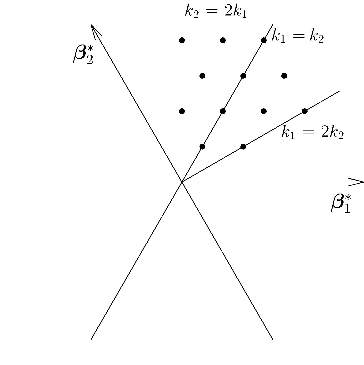
Figure 1: Root diagram for SU(3) showing magnetic weights allowed by (2).

The monopole charge is given by the first Chern class,

$$q\,=\,\lim_{R\to\infty}\int_{\rho=R}\frac{\text{tr}(\hat{F}\hat{\Phi})}{4\pi\|\hat{\Phi}\|}$$ (4)

where integration is over the 2-torus at radial infinity, the length of the Higgs field is $\|\hat{\Phi}\|^{2}=-\frac{1}{2}\text{tr}(\hat{\Phi}^{2})$ and $\text{tr}(\cdot)$ denotes the trace in the Lie algebra. For the $i^{\text{th}}$ fundamental monopole this evaluates to $q=k_{i}$. It is possible to convert between the elements of $\bm{\ell}$ and those of $\bm{k}$ using

$$k_{j}\,=\,\sum_{i=1}^{j}\ell_{i}\qquad\text{and}\qquad\ell_{i}\,=\,k_{i}-k_{i-1},$$

and we define $K=\text{max}(\{k_{i}\})$. We will often refer to a specific class of $\text{SU}(N)$ monopole simply by its $(N-1)$-dimensional charge vector $\bm{k}$.

As is done for monopoles in $\mathbb{R}^{3}$ [8, 9, 10], fundamental monopole masses are defined by the pattern of symmetry breaking of the leading terms in $\hat{\Phi}$. In particular, the $i^{\text{th}}$ mass is

$$m_{i}\,=\,\ell_{i}-\ell_{i+1}$$

where an interpretation as a physical mass requires the specification of a radial cut off. If all the masses are non-zero, the SU($N$) symmetry is maximally broken by the asymptotic Higgs field to $\text{U}(1)^{N-1}$. Otherwise, there may be unbroken subgroups according to whether the corresponding $\mathfrak{v}_{i}$ are the same. We will see examples of this in section 5.2.

Applying (4) to the $\mathfrak{su}(N)$-valued fields, the total charge, $q$, is given by the product of fundamental charges and masses,

$$q^{2}\,\propto\,\sum_{i=1}^{N}\ell_{i}^{2}\,=\,\sum_{i=1}^{N-1}k_{i}m_{i}.$$

A similar result holds for SU($N$) monopoles in $\mathbb{R}^{3}$, although it is noteworthy that in contrast to the $\mathbb{R}^{3}$ case both the charges and masses are now determined from the leading asymptotic term in $\hat{\Phi}$. Consequently, a given pattern of symmetry breaking can only be achieved by a particular choice of fundamental charges. In fig. 1, magnetic weights associated with minimal symmetry breaking are those lying on the lines $k_{1}=2k_{2}$ and $k_{2}=2k_{1}$. This configuration is considered further in section 5.

As pointed out in [1], the total energy is logarithmically divergent, such that the Bogomolny bound is

$$E\,=\,\frac{1}{2}\int_{\mathbb{R}^{2}\times\hat{S}^{1}}\text{tr}(\ast\hat{D}\hat{\Phi}\wedge\hat{D}\hat{\Phi})\,=\,\frac{1}{2}\int_{\rho=R}\text{tr}(\hat{\Phi}\ast\hat{D}\hat{\Phi})\,=\,\frac{\pi}{\beta}\sum_{i=1}^{N}\ell_{i}\left(\ell_{i}\log(R)+v_{i}\right)$$ (5)

and we understand the Bogomolny equations to give a solution which minimises the energy in a region with $R$ large but finite.

As is done for the periodic instanton [11], it is useful to consider the holonomy in the periodic direction. Explicitly, we are to solve the matrix equation

$$\partial_{z}V(\zeta,z)\,=\,\hat{\phi}\,V(\zeta,z)$$ (6)

with boundary condition $V(\zeta,0)=\bm{1}_{N}$, for $V(\zeta,\beta)$. Under a gauge transformation with $\hat{g}=\hat{g}(\zeta,z)\in\text{SU}(N)$, the fields and holonomy transform as rcl ^Φ &↦ ^g^-1^Φ^g
^A ↦ ^g^-1^A^g+^g^-1d^g
V(ζ,z) ↦ ^g^-1(ζ,z)V(ζ,z)^g(ζ,0), where $\hat{g}(\zeta,0)$ is introduced to ensure the boundary condition on $V(\zeta,z)$ is satisfied. As long as $\hat{g}$ is strictly periodic, $\hat{g}(\zeta,\beta)=\hat{g}(\zeta,0)$, then the characteristic polynomial of $V(\zeta,\beta)$ is gauge invariant. Asymptotically, using (3), the holonomy takes the form

$$V(\zeta,\beta)\,=\,\text{diag}\left(\zeta^{\ell_{1}}\text{e}^{\mathfrak{v}_{1}}(1+\mu_{1}\zeta^{-1}+\mathcal{O}(\rho^{-2})),\ldots\right).$$ (7)

The analysis of the Bogomolny equations provided by [1] establishes that the holonomy is in fact holomorphic, and is thus a polynomial in $\zeta$.

1.2 Nahm Transform

It is shown in [12, 13] that the Nahm transform provides a bijection between self-dual Yang-Mills fields on the torus $\hat{T}^{4}$ and the reciprocal torus $T^{4}$. It is believed [6] that other self-dual Yang-Mills systems can be obtained by suitable rescalings of the tori. In the present case, it is therefore expected that the Nahm dual to the monopole on $\mathbb{R}^{2}\times\hat{S}^{1}$ is a Hitchin system [14] on the ‘Hitchin cylinder’ $\mathbb{R}\times S^{1}$ of period $2\pi/\beta$, and this was shown by [1] to be the case. Following the notation of [5, 4] the cylinder is parametrised by the coordinates $r\in\mathbb{R}$ and $t\in\mathbb{R}/(2\pi/\beta)\mathbb{Z}$, which are combined into a complex coordinate $s=r+\text{i}t$. The Hitchin fields are of matrix rank $K$ and satisfy

$$F_{s\bar{s}}\,=\,-\tfrac{1}{4}[\Phi,\Phi^{\dagger}]\qquad\qquad D_{\bar{s}}\Phi\,=\,\partial_{\bar{s}}\Phi+[A_{\bar{s}},\Phi]\,=\,0$$ (8)

with ^† denoting Hermitian conjugation. The monopole fields are recovered, up to a gauge, by finding solutions of the inverse Nahm equation,

$$\Delta\Psi\,=\,\begin{pmatrix}\bm{1}_{K}\otimes(2\partial_{\bar{s}}-z)+2A_{\bar{s}}&\bm{1}_{K}\otimes\zeta-\Phi\\ \bm{1}_{K}\otimes\bar{\zeta}-\Phi^{\dagger}&\bm{1}_{K}\otimes(2\partial_{s}+z)+2A_{s}\end{pmatrix}\,\Psi\,=\,0$$ (9)

where $\Psi$ is a $(2K\times N)$ matrix subject to the normalisation condition

$$\int_{-\infty}^{\infty}\text{d}r\int_{-\pi/\beta}^{\pi/\beta}\text{d}t\,(\Psi^{\dagger}\Psi)\,=\,\bm{N}_{2}.$$ (10)

One can then, in principle, construct the monopole fields using

$$\hat{\Phi}\,=\,\text{i}\int_{-\infty}^{\infty}\text{d}r\int_{-\pi/\beta}^{\pi/\beta}\text{d}t\,(r\Psi^{\dagger}\Psi)\qquad\qquad\hat{A}_{i}\,=\,\int_{-\infty}^{\infty}\text{d}r\int_{-\pi/\beta}^{\pi/\beta}\text{d}t\,(\Psi^{\dagger}\partial_{i}\Psi).$$

Gauge transformations $\hat{g}$ acting on the $\text{SU}(N)$ monopole fields and $g$ on the Nahm fields transform $\Psi$ as

$$\Psi(s;\zeta,z)\,\mapsto\,U(s)^{-1}\Psi(s;\zeta,z)\,\hat{g}(\zeta,z).$$ (11)

where $U(s)=h\otimes g(s)$, with $h$ a constant $2\times 2$ matrix serving to permute the entries in $\Delta$ and those of $\Psi$. This freedom to rearrange makes it evident that it is irrelevant whether the derivatives $\partial_{r}$ and $\partial_{t}$ are introduced in the same or different entries of $\Delta$, the two configurations differing only by a choice of gauge.

Finally, it should be noted that in the $\beta\to 0$ limit the Nahm transform is expected to be self-reciprocal, mapping between two Hitchin systems of different rank and boundary conditions.

1.3 Spectral Data

The key observation of [1, 3] is that the characteristic equation of the $z$-holonomy, $\text{det}(w-V)=0$, relates monopole data to Nahm data through the parameter $w=\text{e}^{\beta s}$. This provides a holomorphic curve S in $\mathbb{C}\times\mathbb{C}^{\ast}$ known as the monopole spectral curve, which for an SU($N$) periodic monopole of charge $\bm{k}$ is

$$w^{N}+P_{1,k_{1}}(\zeta)w^{N-1}+\ldots+P_{N-1,k_{N-1}}(\zeta)w+(-1)^{N}\,=\,0$$ (12)

where the $P_{i,k_{i}}(\zeta)$ denote polynomials in $\zeta$ with leading term proportional to $\zeta^{k_{i}}$. This relation shows that by performing a coordinate redefinition $w\mapsto w^{-1}$ the largest of the $k_{i}$ (if it is unique) can be chosen to lie in the first half of the entries in $\bm{k}$. Referring to the SU($3$) case (fig. 1), this amounts to identifying the regions on either side of the line $k_{1}=k_{2}$, and we will choose to work with the configurations below that line.

In addition to the monopole spectral curve (12), Cherkis & Kapustin [1, 3] introduce a second, equivalent, spectral curve relating the coordinate on $\mathbb{R}^{2}$ in the monopole space to the characteristic equation of the Hitchin Higgs field $\Phi$,

$$\zeta^{K}-\text{tr}(\Phi)\zeta^{K-1}+\ldots+(-1)^{K}\text{det}(\Phi)\,=\,0,$$ (13)

where the intermediate terms are given by symmetric polynomials in the eigenvalues of $\Phi$. By rewriting (12) as a polynomial in $\zeta$, a comparison can be made with the coefficients of (13) to obtain $\Phi$. In particular, it should be noted that $\text{det}(\Phi)$ will have singularities at finite $|r|$ if $K$ appears more than once in $\bm{k}$. Smooth behaviour at large $|r|$ requires the introduction of singularities, both to the monopole and Hitchin fields.

1.4 String Theory Setting

The relation of periodic monopoles to compactified supersymmetric gauge theories is explained in detail in [1, 3, 15] and provides a physical context for the root structure presented in section 1.1. The type IIB setup of interest consists of $N$ parallel D5-branes extended along the $x^{0}$-$x^{5}$ directions and $(N-1)$ stacks of $k_{i}$ D3-branes extended along the $x^{0}$-$x^{2}$ and $x^{6}$ directions ending on each of the $i^{\text{th}}$ pair of adjacent D5-branes, where $x^{3}$ is compactified on a circle. From the point of view of the D5-brane system, each of the D3-branes is seen as a fundamental SU(2) periodic monopole of type $i$ localised in the $x^{3}$-$x^{5}$ directions of the D5-brane worldvolume, and translationally invariant along $x^{0}$-$x^{2}$. Performing a $T$-duality in the $x^{3}$ direction returns a IIA system of D4-branes extended along $x^{0}$-$x^{3}$, $x^{6}$, ending on $N$ other D4-branes extended along $x^{0}$-$x^{2}$, $x^{4}$, $x^{5}$. The field equations on the ($x^{3}$, $x^{6}$)-cylinder are nothing other than the Hitchin equations of section 1.2. The tension between the D4-branes causes them to deform, such that the $x^{6}$ direction of the cylinder becomes of infinite extent.

	0	1	2	​\small{3}⃝​	4	5	6	7	8	9
D5	x	x	x	x	x	x
D3	x	x	x				x

$T_{3}\left\downarrow\rule{0.0pt}{17.07182pt}\right.\phantom{T_{3}}$

	0	1	2	​\small{3}⃝​	4	5	6	7	8	9
D4	x	x	x		x	x
D4	x	x	x	x			x

Introducing $n_{+}$ and $n_{-}$ semi-infinite D3-branes ending on the first and $N^{\text{th}}$ D5-branes is equivalent to the introduction of Dirac singularities to the monopole system. Compactifying the $x^{6}$ direction, such that the left and right D3-branes coincide, is equivalent to adding an $N^{\text{th}}$ root to the Lie algebra $\mathfrak{su}(N)$. The series of dualities described above then leads to Hitchin equations on the 2-torus ($x^{3}$, $x^{6}$). Such a system of singular monopoles and the relation of the torus to the Nahm data of the doubly periodic instanton will be discussed in section 6.

2 Introducing the Spectral Approximation

Due to the difficulty of finding exact solutions to the inverse Nahm operator (9) and motivated by Ward’s approximate $\bm{k}=(1)$ solution [4], we will consider a construction based on the spectral curves (12, 13). The following pargraphs describe the procedure to be followed and in the remainder of this section we use the results of [4] to illustrate the application and régime of validity of the approximation.

Given an SU($N$) monopole with charge vector $\bm{k}$ it is straightforward to write down the spectral curves (12) and (13), where the polynomials $P_{i,k_{i}}(\zeta)$ can be expressed in terms of the data $\bm{\mathfrak{v}}$, $\bm{\mu}$. We will be interested in the ‘spectral points’, those values of $\zeta$ at which two or more of the eigenvalues of $V(\zeta,\beta)$ coincide. These points are located by finding the zeroes of the discriminant $\mathcal{D}_{\bm{k}}$ of the polynomial in $w$ (as a function of $\zeta$). For given $N$, the discriminant is obtained as the determinant of the rank $(2N-1)$ Sylvester matrix. Our interest in the spectral points stems from the finding in the $\bm{k}=(1)$ case, discussed in section 2.1, that peaks in energy density are always located at the spectral points (though there appears to be no energy peak associated to two coincident spectral points, as will be seen for $\bm{k}=(2)$ in section 3.3). It can be checked by explicit calculation for small $N$ that the highest power of $\zeta$ in $\mathcal{D}_{\bm{k}}$ is $2\sum_{i=1}^{N-1}k_{i}$, and we expect there to be this many spectral points. We will see from various examples that away from the central region of the moduli space, the spectral points occur in pairs, forming $\sum_{i=1}^{N-1}k_{i}$ fundamental monopoles.

The spectral curve (12) of the SU($N$) charge $\bm{k}$ periodic monopole has $2\sum_{i=1}^{N-1}(k_{i}+1)$ real coefficients. It is expected [3] that the complex coefficient of $\zeta^{k_{i}}$ in each of the polynomials $P_{i,k_{i}}(\zeta)$ is a parameter determined by the boundary data $\bm{\mathfrak{v}}$. The centre of mass of the spectral points is factored out by choosing $\bm{\mu}$ such that the term of order $\zeta^{2\sum k_{i}-1}$ in $\mathcal{D}_{\bm{k}}$ vanishes, and we will say that such a monpole is centered. Overall, this yields $2\sum_{i=1}^{N-1}k_{i}-2$ real relative moduli, precisely half the number expected were we to consider the full three dimensional picture. This suggests our approach is insensitive to relative $z$ and phase differences between the fundamental monopoles, such that its validity is expected to improve as the ratio of the monopole size to its period becomes large. We will refer to the moduli appearing in the spectral curve as ‘reduced moduli’, and will see in section 4 that in the SU(2) charge $\bm{k}=(2)$ case they provide a geodesic submanifold of the full moduli space.

2.1 SU(2) Charge 1 - Spectral Curve

We illustrate the procedure by reviewing the approximate construction of [4] for $\bm{k}=(1)$. The spectral curves in this case are (recall that $\Phi$ is a matrix of rank $1$)

$$w^{2}-2(\zeta-a)w/C+1\,=\,0\qquad\qquad\zeta-\Phi\,=\,0.$$ (14)

The boundary data translates to $C=2\text{e}^{-\mathfrak{v}}$, $a=-\mu$, such that the Hitchin Higgs field is

$$\Phi\,=\,a+C\cosh(\beta s)$$

while the Hitchin gauge potential $A_{r}$ can be set to zero by a gauge transformation and the Hitchin equations (8) are satisfied trivially. The inverse Nahm transform (9) requires a solution of

$$\begin{pmatrix}2\partial_{\bar{s}}-z&\zeta-\Phi\\ \bar{\zeta}-\Phi^{\dagger}&2\partial_{s}+z\end{pmatrix}\begin{pmatrix}\Psi_{+}\\ \Psi_{-}\end{pmatrix}\,=\,0$$ (15)

(such that $A_{t}$ is absorbed into $z$ and $a$ into $\zeta$). For $(\zeta,\text{e}^{\beta s_{0}})\in\text{\bf{S}}$, $(\zeta-\Phi)$ will vanish at

$$\beta s\,=\,\pm\beta s_{0}\,=\,\pm\cosh^{-1}\left((\zeta-a)/C\right),$$ (16)

such that away from the spectral curve,

$$\zeta-\Phi\,=\,\pm\beta C(s\pm s_{0})\sinh(\beta s_{0})+\mathcal{O}(s\pm s_{o})^{2}\,=\,\pm\beta(s\pm s_{0})\xi+\mathcal{O}(s\pm s_{o})^{2}$$

where $\xi^{2}=\zeta^{2}-C^{2}$. As suggested by [4], solutions to (15) are supported near the points $s=\pm s_{0}=\pm(r_{0}+\text{i}t_{0})$ on the Hitchin cylinder. The independent solutions take the form of Gaussian peaks localised at each of $\pm s_{0}$, assembled into

$$\Psi\,\approx\,\mathcal{N}\begin{pmatrix}\xi E_{-}&|\xi|E_{+}\\ -|\xi|E_{-}&\bar{\xi}E_{+}\end{pmatrix}$$

where

$$\log(E_{\pm}(s))\,=\,-\tfrac{1}{2}\beta|\xi|\left((r\pm r_{0})^{2}+(t\pm t_{0})^{2}\right)-\text{i}zt$$

and we have chosen a different gauge to [4], such that the monopole fields are traceless and explicitly independent of $z$. Such a solution is valid when the peaks on $\mathbb{R}\times S^{1}$ are well separated, and narrow compared to the period of the cylinder. These conditions are ensured if we stay away from the spectral points $\zeta=\pm C$,

$$|\zeta^{2}-C^{2}|\,\gg\,\frac{\beta^{2}}{16\pi^{2}}.$$ (17)

In this region, the normalisation factor $\mathcal{N}$ is determined from (10) to be $|\mathcal{N}|^{2}=\beta/(2\pi|\xi|)$ and the monopole fields, after a gauge transformation $\hat{g}=\text{exp}(\frac{1}{4}\log(\bar{\xi}/{\xi})\sigma_{3})$ are

$$\hat{\Phi}\,=\,\text{i}r_{0}\sigma_{3}\qquad\qquad\hat{A}_{z}\,=\,-\text{i}t_{0}\sigma_{3}$$ (18)

$$\hat{A}_{\zeta}\,=\,\frac{\zeta}{4\xi^{2}}\,\text{e}^{-\beta|\xi||s_{0}|^{2}}\sigma_{1}\qquad\qquad\hat{A}_{\bar{\zeta}}\,=\,-\hat{A}_{\zeta}^{\dagger}$$

where to ensure we remain on the correct branch we choose

$$|s_{0}|^{2}\,=\,\inf_{n\in\mathbb{Z}}\left(r_{0}^{2}+(t_{0}+n/2)^{2}\right).$$

It is important to note that the fact the monopole Higgs field can be read off directly from the spectral curve (14) via $s_{0}$ (16) is not simply a restatement of the boundary conditions, as use has also been made of the fact the coefficients in $w$ of the spectral curve are polynomials in $\zeta$, which encode the moduli in a particular way [3]. This result will be used in sections 3, 5 and 6 when we discuss the charge $2$, SU(3) and singular periodic monopoles.

It is useful to combine the fields (18) into $\text{i}\hat{\phi}=\hat{\Phi}-\text{i}\hat{A}_{z}$ and $\hat{a}=\hat{A}_{\zeta}\text{d}\zeta+\hat{A}_{\bar{\zeta}}\text{d}\bar{\zeta}$ (see (3)). We note that $\hat{a}$ approaches zero exponentially away from the spectral points $\zeta=\pm C$, and the fields are Abelian and trivially satisfy Hitchin equations in this limit, suggesting that they are truly two dimensional. Noting that $|s_{0}|$ has dimensions of $\beta^{-1}$, we conjecture that in the limit $\beta\to 0$ a solution is provided by

$$\hat{\phi}\,=\,s_{0}\sigma_{3}\qquad\qquad\hat{a}\,=\,0,$$

which satisfies the Bogomolny equations with the correct boundary conditions (3). As will be seen in section 3.4, this approximation also leads to the correct asymptotic behaviour of the moduli space.

2.2 Charge 1 - Energy

It is convenient to rewrite the energy density, the integrand of (5) in terms of just the Higgs field by using the Bianchi identity [9, 16],

$$\mathcal{E}\,=\,\tfrac{1}{4}\,\nabla^{2}\,|\text{tr}(\hat{\Phi}^{2})|.$$ (19)

The Higgs field (18) is

$$\hat{\Phi}\,=\,\frac{\text{i}}{\beta}\,\Re\left(\cosh^{-1}\left(\frac{\zeta}{C}\right)\right)\sigma_{3}\,=\,\frac{\text{i}}{\beta}\,\log\left|\frac{\zeta}{C}+\sqrt{\left(\frac{\zeta}{C}\right)^{2}-1}\right|\sigma_{3},$$ (20)

giving an energy density

$$\mathcal{E}_{1}\,=\,\frac{1}{\beta^{2}|\xi|^{2}}\,=\,\frac{1}{\beta^{2}}\frac{1}{\sqrt{\rho^{4}-2\rho^{2}C^{2}\cos(2\theta)+C^{4}}}$$ (21)

whose contours trace out Cassini ovals (fig. 2) and is peaked at the spectral points, whose separation by $2C$ allows us to interpret $C$ as the characteristic size of the monopole.

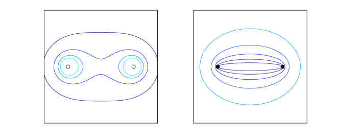
Figure 2: An SU(2) monopole. On the left is a contour plot of the energy density (21) and on the right $\log(\text{disc}(\hat{\Phi})+0.001)$, where the discriminant is defined as the squared difference of the eigenvalues of $\hat{\Phi}$. It is zero on a line joining the spectral points, whose locations are indicated by black dots on the right hand diagram. Note the loss of axial symmetry.

We next use the divergence theorem to compute the total energy in a region with $\rho=R\gg C$

$$V_{1}\,=\,\tfrac{1}{4}\int\!\!\!\!\int\!\!\!\!\int_{\rho\leq R}\nabla^{2}|\text{tr}(\hat{\Phi})^{2}|\rho\text{d}\rho\text{d}\theta\text{d}z\,=\,\tfrac{1}{4}R\beta\int_{\rho=R}\left(\partial_{\rho}|\text{tr}(\hat{\Phi})^{2}|\right)\text{d}\theta$$

and note that the leading term of the integrand at large $\rho$ is

$$\partial_{\rho}|\text{tr}(\hat{\Phi})|^{2}\,\sim\,\frac{4}{\rho\beta^{2}}\log\left(\frac{2\rho}{C}\right),$$

resulting in

$$V_{1}\,=\,\int\!\!\!\!\int\!\!\!\!\int_{\rho\leq R}\mathcal{E}_{1}\rho\text{d}\rho\text{d}\theta\text{d}z\,=\,\frac{2\pi}{\beta}\log\left(\frac{2R}{C}\right)$$

in agreement with (5). Finally, we note that the Higgs field (20) vanishes along a line between the spectral points, fig. 2, as can be seen in the numerical study of [17]. We will see in section 6 that this observation survives for higher charges.

3 Charge 2 - Spectral Approximation

In this section we apply the spectral approximation to the SU(2) monopole of charge $\bm{k}=(2)$, which has two real reduced moduli. Using symmetries of the spectral curves this can be reduced to two one-parameter families, though we withhold showing that this two dimensional reduced moduli space is itself a geodesic submanifold of the full four dimensional moduli space until section 4.2.

In the limit in which the approximation becomes exact it is possible to compute a metric on the two dimensional reduced moduli space. Its asymptotic form agrees with the ALG metric of [2], allowing numerical integration of non-trivial geodesics, which will be considered both in the monopole space and on the dual cylinder. Finally, we will introduce a new solution of the rank $2$ Hitchin system [18] with the same spectral limit as that of [5], and briefly compare their scattering properties.

3.1 Spectral Approximation

The general form of the monopole spectral curve (12) of the charge $\bm{k}=(2)$ periodic monopole is

$$w^{2}+P_{1,2}(\zeta)w+1\,=\,0\qquad\text{with}\qquad P_{1,2}(\zeta)\,=\,-\left(2\zeta^{2}-2BC\zeta-K\right)/C.$$ (22)

where $B,C\in\mathbb{C}$. The spectral points are located at the values of $\zeta$ where $(P_{1,2}(\zeta))^{2}=4$. Fixing the centre of mass at the origin, we expect energy peaks at the four points

$$\zeta\,=\,\pm\sqrt{K/2\pm C}$$

(where the $\pm$ signs are independent). As in the $\bm{k}=(1)$ case, $C$ is a parameter fixed by the boundary conditions, while $K$ is a complex modulus. For $|K|\gg 2|C|$ the spectral points occur in two pairs which are interpreted as fundamental monopoles of size $|C\sqrt{2/K}|$ separated by a distance $|\sqrt{2K}|$. It is noteworthy that the fundamental monopoles get smaller as they are separated, an effect of the long range Higgs field.

Motivated by (18) we assume the monopole Higgs field is given by $\hat{\Phi}=\text{i}\Re(s_{0})\sigma_{3}$, where $s_{0}$ is obtained by rearranging the spectral curve,

$$\hat{\Phi}\,=\,\frac{\text{i}}{\beta}\,\Re\left(\cosh^{-1}\left(\frac{2\zeta^{2}-K}{2C}\right)\right)\sigma_{3}$$

and compute the energy in a region with $|\zeta|<R$ using (19) to find

$$V_{2}\,=\,\frac{4\pi}{\beta}\log\left(\frac{2R^{2}}{C}\right),$$

again in agreement with (5). Applying the divergence theorem to $\partial_{K}\mathcal{E}$ for large $\rho$,

$$\partial_{K}\mathcal{E}\,\propto\,\partial_{K}\partial_{\rho}|\text{tr}(\hat{\Phi}^{2})|\,\sim\,\rho^{-3}\log(\rho),$$

shows that, as hoped, the total energy is independent of the modulus $K$.

3.2 Aside - Symmetric Charge k

The spectral curve of the $\mathbb{Z}_{2k}$-symmetric charge $\bm{k}=(k)$ monopole is

$$C\cosh(\beta s)\,=\,\zeta^{k}\qquad\Rightarrow\qquad\hat{\Phi}\,=\,\frac{\text{i}}{\beta}\,\Re\left(\cosh^{-1}\left(\frac{\zeta^{k}}{C}\right)\right)\sigma_{3},$$

from which the energy density (21) is

$$\mathcal{E}_{k}\,=\,\frac{k^{2}}{\beta^{2}}\frac{\rho^{2k-2}}{\sqrt{\rho^{4k}-2C^{2}\rho^{2k}\cos(2k\theta)+C^{4}}},$$

where we note that the energy density at the origin vanishes for all $k>1$.

The total energy is again in agreement with (5), while the energy per unit charge in the region $0\leq\rho\leq aC^{1/k}$ is (note that the spectral points are located on a circle of radius $\rho=C^{1/k}$) rcl Vkk (0≤ρ≤aC^1/k) &= πa2kβ​​​​F_3F_2(12,12,12;1,32;a^4k)
= {πa^2k(1+O(a^4k))/β(a¡1)4G/β(a=1) where $\!\!\!\!\phantom{F}{}_{3}F_{2}$ is the generalised hypergeometric function, $G\approx 0.916$ is Catalan’s constant and we have used the following identities for the elliptic integral $\bm{K}(\kappa)$ [19]:

$$\bm{K}(\kappa)\,=\,\int_{0}^{\pi/2}\frac{1}{\sqrt{1-2\kappa\cos(2\alpha)+\kappa^{2}}}\,\text{d}\alpha\qquad\qquad(\kappa<1),$$

$$4ab\int_{0}^{z}\kappa^{2ab-1}\bm{K}(\kappa^{b})\,\text{d}\kappa\,=\,\pi z^{2ab}\!\!\!\!\phantom{F}_{3}F_{2}\left(\tfrac{1}{2},\tfrac{1}{2},a;1,a+1;z^{2b}\right).$$ (23)

Fig. 3 shows the total energy in a period cylinder, (3.2), is increasingly located at its edge as $k$ is increased. An expansion of the fields at small and large $\rho$ yields

$$\left\{\begin{array}[]{lll}-\text{i}\beta\hat{\Phi}\,\sim\,(\rho^{k}/C)\sin(k\theta)\sigma_{3}&&(\rho^{k}\ll C),\\ -\text{i}\beta\hat{\Phi}-\log\left(2\rho^{k}/C\right)\sigma_{3}\,\sim\,(2\rho^{k}/C)^{-2}\cos(2k\theta)\sigma_{3}&&(\rho^{k}\gg C).\end{array}\right.$$

These results resemble those found for spherical magnetic bags of large charge, as first studied by [20], and it is interesting to see evidence of a ‘magnetic cylinder’ with similar properties.

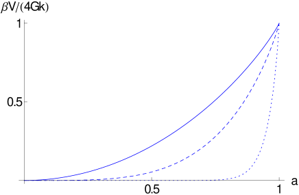
Figure 3: Normalised energy per unit charge enclosed in a period cylinder of radius $aC^{1/k}$ for various values of the charge $k$. Solid line: $k=1$, dashed: $k=2$, dotted: $k=10$. The energy density is increasingly located on a shell of radius $\rho=C^{1/k}$.

3.3 Symmetries

Geodesic submanifolds of the two dimensional reduced moduli space are obtained by looking for symmetries in the spectral curve (22). Fixing the parameters $B=0$ and $C\in\mathbb{R}$, we impose invariance of (22) under a reflection symmetry in the line $\theta=\alpha/2$, encoded by the map $\zeta\mapsto\text{e}^{\text{i}\alpha}\bar{\zeta}$. This requires that we simultaneously map $w\mapsto\text{e}^{-2\text{i}\alpha}\bar{w}$ ($t\mapsto-t-2\alpha/\beta$) and $K\mapsto\text{e}^{2\text{i}\alpha}\bar{K}$. The original spectral curve (22) is recovered by complex conjugation as long as $\alpha$ is chosen to be $0$ or $\pi/4$. These choices of $\alpha$ correspond to the one parameter families $K\in\mathbb{R}$ and $K\in\text{i}\mathbb{R}$, respectively. In section 4 it will be shown that the reduced moduli provide a geodesic submanifold of the full four dimensional moduli space, allowing us to consider the above one parameter families as geodesics. The definition of a metric on the reduced moduli space will be considered in the following subsection.

More information about these geodesics can be gleaned from considering the $\pi/2$ rotation symmetry $\zeta\mapsto\mathrm{i}\zeta$, which requires $w\mapsto-w$ ($t\mapsto t+\pi/\beta$) and $K\mapsto-K$. For the one parameter families found above, passing through $K=0$ leads to the right-angled scattering processes shown in fig. 4. Particularly interesting points in the moduli space are $K=\pm 2C$, where two of the spectral points coincide at the origin (although there is no energy peak associated with them) and $K=0$, where the dihedral $D_{2}$ symmetry is enhanced to $D_{4}$. This is nothing but the symmetric configuration considered in section 3.2. For $K/C\in[-2,2]$ the fundamental monopoles lose their individual identities and the discriminant vanishes on a cross shape joining the four peaks.

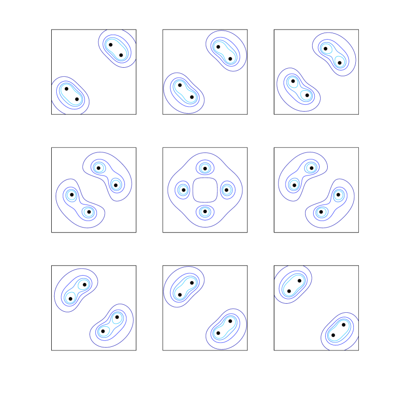
Figure 4: Energy density contour plots. Left: geodesic with $K\in\mathbb{R}$ (to be read from left to right and top to bottom). Right: geodesic with $K\in\text{i}\mathbb{R}$. The central symmetric configurations have $K=0$, while those with just two energy peaks have $K=\pm 2$. It is noteworthy that the axial symmetry of the ‘doughnut’ charge $2$ monopole in $\mathbb{R}^{3}$ is replaced by a discrete symmetry. The spacing between snapshots is taken relative to the metric defined in section 3.4.

3.4 Metric

3.4.1 Definition

We use the general formalism for obtaining the moduli space metric from the variation of the fields (see, for example, [9]). For $z$-independent fields the metric is given by

$$g\,=\,\tfrac{1}{2}\dot{K}\dot{\bar{K}}\int_{\mathbb{R}^{2}}\text{tr}\left(\partial\hat{\phi}\bar{\partial}\hat{\phi}^{\dagger}+\partial\hat{\phi}^{\dagger}\bar{\partial}\hat{\phi}-4\partial\hat{a}_{\bar{\zeta}}\bar{\partial}\hat{a}_{\zeta}-4\partial\hat{a}_{\zeta}\bar{\partial}\hat{a}_{\bar{\zeta}}\right)\text{d}^{2}x$$

where it is understood that the fields satisfy the gauge condition

$$2\left(D_{\zeta}\partial(\hat{a}_{\bar{\zeta}})+D_{\bar{\zeta}}\partial(\hat{a}_{\zeta})\right)\,=\,\tfrac{1}{2}[\hat{\phi},\partial(\hat{\phi}^{\dagger})]+\tfrac{1}{2}[\hat{\phi}^{\dagger},\partial\hat{\phi}]$$ (24)

which arises as a dimensional reduction of the equivalent condition for instantons, $D_{\mu}(\partial A_{\mu})=0$. Here $\partial$ indicates differentiation with respect to $K$, and $\dot{}$ is differentiation with respect to an affine time $\tau$.

From (18) there is a centered charge $2$ solution of the Bogomolny equations with

$$\beta\hat{\phi}\,=\,\cosh^{-1}\left(\frac{2\zeta^{2}-K}{2C}\right)\sigma_{3}\qquad\qquad\hat{a}\,=\,0,$$

valid sufficiently far from the spectral points, for which the orthogonality condition (24) holds trivially. As discussed in section 2.1, it will be assumed that this becomes exact in the limit of $z$-independence. It follows that the metric is given by

$$g\,=\,\frac{1}{4\beta^{2}}\dot{K}\dot{\bar{K}}\int\left((\zeta^{2}-K/2)^{2}-C^{2}\right)^{-1/2}\left((\bar{\zeta}^{2}-\bar{K}/2)^{2}-C^{2}\right)^{-1/2}\,\rho\text{d}\rho\text{d}\theta.$$ (25)

For given $K$ the integral can be written in terms of products of distances to the four spectral points, which are located at $\zeta_{i}(K)=\pm\sqrt{K/2\pm C}$, defining the conformal factor $\eta(K)$,

$$g\,=\,\frac{1}{4\beta^{2}}\dot{K}\dot{\bar{K}}\int\frac{1}{|\zeta-\zeta_{1}||\zeta-\zeta_{2}||\zeta-\zeta_{3}||\zeta-\zeta_{4}|}\,\rho\text{d}\rho\text{d}\theta\,=\,\eta\dot{K}\dot{\bar{K}}.$$

We note that due to holomorphicity of the Higgs field $\hat{\phi}$ the moduli space is a one-complex-dimensional Hermitian manifold. As expected for a complex submanifold of the four-real-dimensional hyper-Kähler moduli space [2], $g$ is indeed Kähler, with Kähler potential proportional to $\int|\text{tr}(\hat{\phi}^{2})|\rho\text{d}\rho\text{d}\theta$.

3.4.2 Asymptotics

The integral in (25) can be computed in the limit in which the monopoles are well separated, $|K|\gg 2|C|$. Two of the peaks are placed near the origin, at $\zeta=\pm\epsilon$, and the others are centered at some large $R$ along the $x$-axis (for simplicity we consider $K=k\text{e}^{\text{i}\alpha}\in\mathbb{R}$). Integrating out to some $\rho_{0}$ ($R\gg\rho_{0}\gg\epsilon$),

$$\eta\,\sim\,\frac{1}{R^{2}}\int_{0}^{\rho_{0}}\frac{1}{|\zeta+\epsilon||\zeta-\epsilon|}\,\rho\text{d}\rho\text{d}\theta.$$

This integrand is identical to that of (21), so

$$\eta\,\sim\,\frac{1}{R^{2}}\log(2\rho_{0}/\epsilon).$$

We recall from section 3.1 that the separation and size of the fundamental monopoles in this limit are, respectively,

$$R\,=\,\sqrt{2k}\qquad\qquad\epsilon\,=\,C(2k)^{-1/2}\,=\,C/R,$$

allowing us to express the metric either in terms of $k$ or the monopole separation $R$,

$$g\,\sim\,\frac{1}{k}\left(\log(k)+c\right)\dot{k}^{2}\,\sim\,\left(\log(R)+c^{\prime}\right)\dot{R}^{2}.$$

The latter agrees, up to prefactors, with the asymptotic metric computed in [2], which is an ALG metric of limiting Gibbons-Hawking type [21]. The constants $c$ and $c^{\prime}$ depend on the upper limit of integration $\rho_{0}$ and are related to the redefinition of $\mathfrak{v}$ performed in [2] when a chain of $n$ monopoles is studied in the limit of $n\to\infty$.

3.4.3 Integration

There are three specific values of $K$ at which evaluation of the conformal factor $\eta$ can be performed analytically (see fig. 4 for the relevant monopole configurations), lll K = 0&    η = 132πβ2C (Γ(14))^4
K → ±2C    η ∼ -π8β2Clog(—K∓2C—) where, for $K=0$, use has been made of (23). The integral diverges at $K=\pm 2C$, when two of the spectral points coincide and there is a double pole in the integrand. We employ these results to ensure a correct numerical implementation of the integral for general $K$, and the result is shown in fig. 5. Further evidence for this metric will be provided in [22].

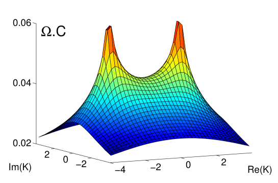
Figure 5: Surface plot of the conformal factor for the relative reduced moduli space in the limit of large monopole size to period ratio. Peaks are at $K=\pm 2C$.

Using polar coordinates $K=k\text{e}^{\text{i}\alpha}$ the geodesic equations are rcl 2ηk^2¨α+(∂_αη)(k^2˙α^2-˙k^2)+2(∂_kη)k^2˙α˙k+4ηk˙α˙k &= 0
2η¨k+(∂_kη)(˙k^2-k^2˙α^2)+2(∂_αη)˙α˙k-2ηk˙α^2 = 0 where $\dot{}$ denotes differentiation with respect to the parameter time $\tau$. In particular, there are geodesics with $\dot{\alpha}=0$, for which the geodesic equations become $\partial_{\alpha}\eta=0$ and

$$2\eta\ddot{k}+(\partial_{k}\eta)\dot{k}^{2}\,=\,0\qquad\Rightarrow\qquad\int\sqrt{\eta}\,\text{d}k\,=\,b_{1}\tau+b_{2},$$ (26)

where $b_{1}$ and $b_{2}$ are constants of integration. As can be seen from fig. 5 such geodesics are only possible for $\alpha=0,\pi/2$, which are precisely the geodesic submanifolds $K\in\mathbb{R}$ and $K\in\text{i}\mathbb{R}$ obtained by symmetry arguments in section 3.3.

The logarithmic behaviour of $\eta$ in the vicinity of $K=\pm 2C$ (3.4.3), combined with the implicit expression for $k(\tau)$ (26), is sufficient to show that geodesics cross the points $K=\pm 2C$ in finite parameter time.

3.4.4 New Geodesics

In complex coordinates the geodesic equations (5) are

$$\eta\ddot{K}+(\partial_{K}\eta)\dot{K}^{2}\,=\,0$$

and its complex conjugate. We write this as a system of coupled partial differential equations,

$$\eta\dot{v}+(\partial_{K}\eta)v^{2}\,=\,0\qquad\qquad\dot{K}\,=\,v$$

and obtain $\partial_{K}\eta$ by differentiating the integrand of $\eta$ before performing the integral (this choice of ordering giving greater numerical precision),

$$\partial_{K}\eta\,=\,\frac{1}{2}\,\int(\zeta^{2}-K/2)\left((\zeta^{2}-K/2)^{2}-C^{2}\right)^{-3/2}\left((\bar{\zeta}^{2}-\bar{K}/2)^{2}-C^{2}\right)^{-1/2}\,\rho\text{d}\rho\text{d}\theta,$$

which must again be integrated numerically. Then, by specifying initial values of $K$ and $\dot{K}$, novel geodesics are integrated using a fourth order Runge-Kutta procedure. Two such non-trivial geodesics are displayed in figs 6 and 7, which are to be compared with those of fig. 4. It is worth noting that geodesics crossing the line segment $-2<K/C<2$ (fig. 6) scatter by swapping constituents, otherwise there is glancing scattering and each fundamental monopole retains its identity (fig. 7). As was seen in fig. 4, a geodesic meeting $K=\pm 2C$ has two coincident spectral points, whose associated energy density vanishes. There is numerical evidence that the only geodesic to cross these points is that with $K\in\mathbb{R}$.

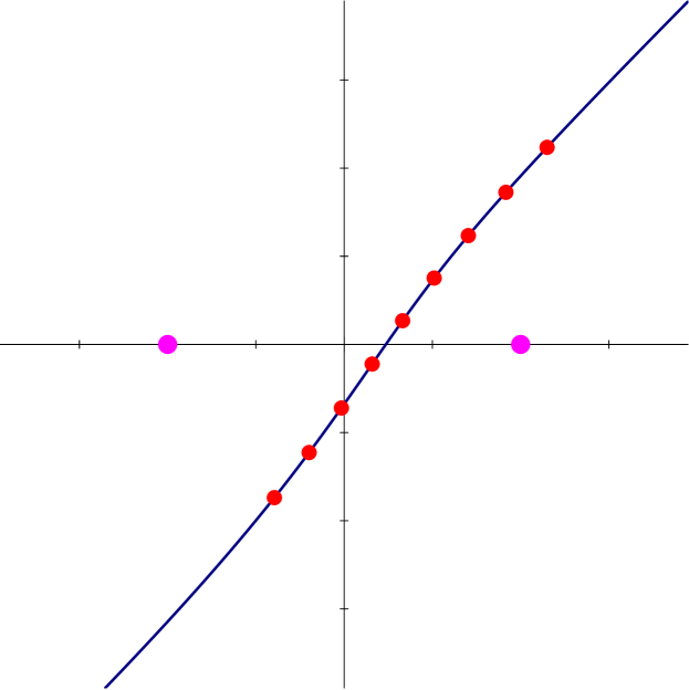
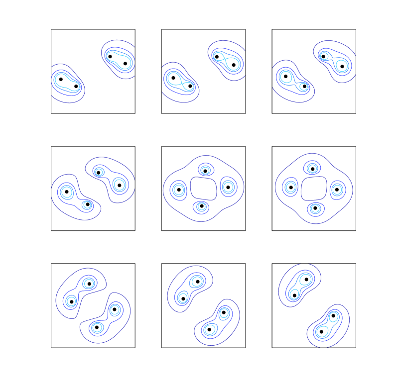
Figure 6: Geodesic for initial condition $K/C=5(1+\text{i})$, $\dot{K}/C=-0.03(1+\text{i})$ with step size $0.03$. The left hand plot displays the geodesic on the $K$-plane (with shaded circles at $K/C=\pm 2$). Tick marks every $722$ timesteps indicate the positions of the energy density snapshots displayed to the right.

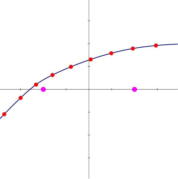
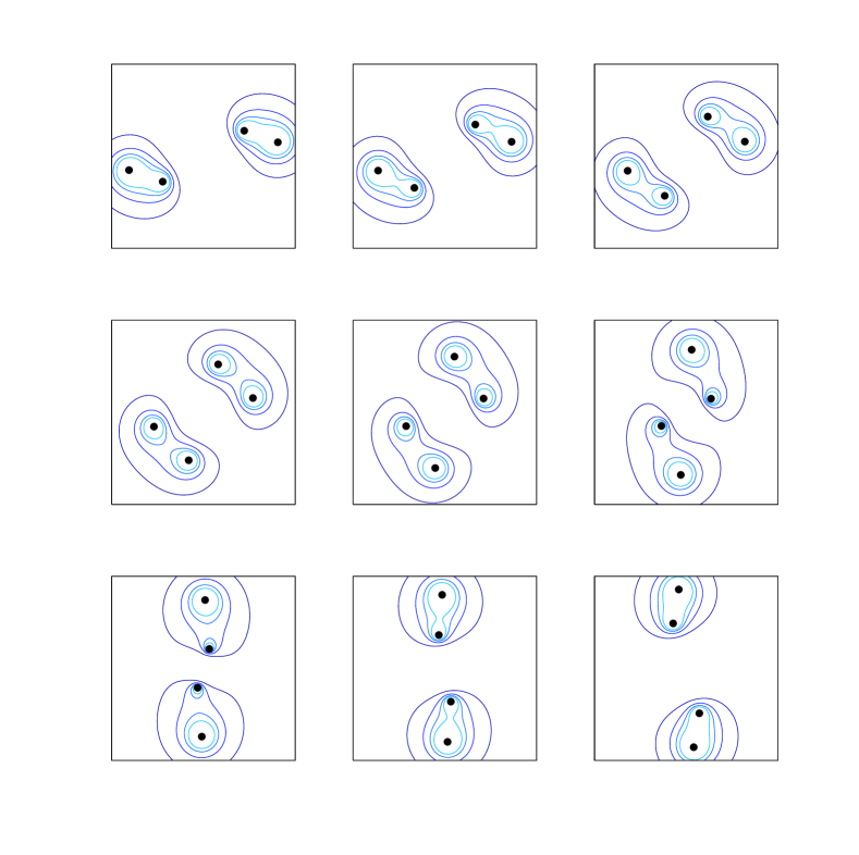
Figure 7: Geodesic for initial conditions $K/C=5+2\text{i}$, $\dot{K}/C=-0.042$ with step size $0.03$. Tick marks are at every $950$ timesteps. In this case the fundamental monopoles retain their separate identities.

3.5 Zeroes on the Cylinder

Rewriting the spectral curve (22) as a polynomial in $\zeta$ and comparing with (13) we find

$$\zeta^{2}-\left(C\cosh(\beta s)+K/2\right)\,=\,0\qquad\Rightarrow\qquad-\text{det}(\Phi)\,=\,C\cosh(\beta s)+K/2.$$

The determinant of the Hitchin Higgs field has two zeroes whose locations on the cylinder depend on $K/C$. In section 4 we will see that these values are of interest as they provide approximate locations for peaks in the gauge field $F_{s\bar{s}}$ on the Hitchin cylinder (8). As $\cosh$ is an even function, the zeroes are always on opposite sides of the cylinder, at $\pm s_{0}$. They are located on the circle $r=0$ if $-2\leq K/C\leq 2$ and coincide at $s_{0}=\text{i}\pi/\beta,0$ if $K/C=2,-2$. This suggests, as was noted in fig. 4, that $K=0$ is a particularly symmetric case, for which the zeroes are at $\pm\text{i}\pi/2\beta$. The motion of the zeroes corresponding to the geodesics with $K\in\mathbb{R}$ and $K\in\text{i}\mathbb{R}$ are shown in figs 8 and 9. Other geodesics lead either to glancing scattering of the zeroes (if $K/C$ passes between $-2$ and $2$, such as in fig. 6) or to them returning in the same direction they come in from (if $K/C$ does not cross the line segment $[-2,2]$, such as in fig. 7).

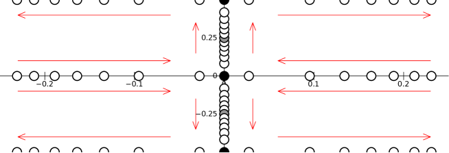
Figure 8: Motion of zeroes on the Hitchin cylinder for $K\in\mathbb{R}$, where the top and bottom edges of the diagram are identified and the $z$ period is taken to be $\beta=2\pi$. Arrows indicate the direction of $K$ increasing from $K/C=-4.5$, with spacing determined by the velocity using the metric (25). The black dots are at $K/C=\pm 2$ (note that in these cases the zeroes coincide), while the grey dots are at $K=0$. Zeroes at the same $K$ are located at opposite points on the cylinder, obtained by reversing the signs of $r$ and $t$.

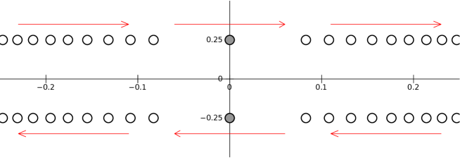
Figure 9: The setup is the same as that of fig. 8, this time with $K\in\text{i}\mathbb{R}$. The arrow indicates the evolution with $\Im(K)$ increasing from $\Im(K)=-4.5$.

4 Charge 2 - Nahm Transform

The centered SU(2) charge $\bm{k}=(2)$ periodic monopole has four real moduli, two of which, as was seen in sections 1.3 and 3.1, are encoded in the spectral curve and describe the relative positions and orientations of the fundamental monopoles in $\mathbb{R}^{2}$. The remaining two moduli are expected to describe the relative phase and $z$ separation. By considering the action of gauge transformations on the inverse Nahm operator (as defined in section 1.2) we will see that the two reduced moduli appearing in the spectral curve provide a geodesic submanifold of the full moduli space. The one parameter families $K\in\mathbb{R}$ and $K\in\text{i}\mathbb{R}$ are studied, and we will find that the details of $z$ behaviour depend on our choice of solution of the Hitchin equations on the Hitchin cylinder. The work in this section is motivated by [5, 18], and it should be noted that the results are independent of the spectral approximation of section 3.

4.1 Hitchin Equations on the Cylinder

The Nahm data of interest are U(2) (or SU(2) if the monopole is centered) Hitchin fields ($\Phi,A$) (8) on the Hitchin cylinder, with $\text{det}(\Phi)$ determined by the spectral curve as described in section 3.5. It is straightforward to show [5] that the Hitchin equations can be solved (up to $\text{U}(1)$ gauge transformations) by

$$\Phi\,=\,\begin{pmatrix}0&\mu_{+}\text{e}^{\psi/2}\\ \mu_{-}\text{e}^{-\psi/2}&0\end{pmatrix}\qquad\qquad A_{\bar{s}}\,=\,a\sigma_{3}+\alpha\Phi\qquad\qquad A_{s}\,=\,-\bar{a}\sigma_{3}-\bar{\alpha}\Phi^{\dagger}$$ (27)

where

$$-\text{det}(\Phi)\,=\,\mu_{+}\mu_{-}\,=\,C\cosh(\beta s)+K/2$$

and $a$, $\alpha$ and $\psi$ are functions of $(s,\bar{s})$ satisfying $4a=-\partial_{\bar{s}}\psi$,

$$\nabla^{2}\Re(\psi)\,=\,2(1+4|\alpha|^{2})\left(|\mu_{+}|^{2}\text{e}^{\Re(\psi)}-|\mu_{-}|^{2}\text{e}^{-\Re(\psi)}\right)$$ (28)

and

$$\text{e}^{-\Re(\psi)/2}\,\partial_{s}\left(\alpha\mu_{+}\text{e}^{\Re(\psi)}\right)+\text{e}^{\Re(\psi)/2}\,\partial_{\bar{s}}\left(\bar{\alpha}\bar{\mu}_{-}\text{e}^{-\Re(\psi)}\right)\,=\,0,$$ (29)

with the imaginary part of $\psi$ chosen in such a way that $\Phi$ has the correct $t$-period.

It is clear that $\alpha=0$ allows (29) to hold trivially, and in the next subsection it will be seen that it in fact provides a two dimensional geodesic submanifold of the relative moduli space. When this is the case, there are two fundamentally different solutions for $\Phi$ according to the allocation of the zeroes of $\text{det}(\Phi)$ between its two non-vanishing components:

• Harland’s solution [18] places both zeroes in the same component,

  $$\mu_{+}\,=\,C\cosh(\beta s)+K/2\qquad\qquad\mu_{-}\,=\,1$$

  with $\Im(\psi)=0$. We call this the ‘zeroes together’ solution.

• On the other hand, Harland & Ward [5] place one zero in each component of $\Phi$,

  $$\mu_{\pm}\,=\,\sqrt{C/2}\left(\text{e}^{\beta s/2}+\lambda^{\pm 1}\text{e}^{-\beta s/2}\right)\qquad\text{where}\qquad 2C\lambda^{\pm 1}\,=\,K\pm\sqrt{K^{2}-4C^{2}}$$

  this time with $\Im(\psi)=\beta t$. This is the ‘zeroes apart’ solution.

For $\alpha=0$ the Hitchin Higgs fields are thus of different matrix rank and there is no smooth gauge transformation between them. As such, the ‘zeroes together’ and ‘zeroes apart’ solutions are disconnected two dimensional submanifolds of the moduli space. It is expected that in the full four dimensional moduli space one can interpolate between the two cases.

4.2 Symmetries

Once the Hitchin equations of section 4.1 have been solved, one should apply the procedure of section 1.2 to obtain the monopole fields. This has been done numerically for the ‘zeroes apart’ case [5]. Here, we consider symmetries of the Nahm transform by means of gauge transformations (11). This is achieved by first looking for transformations of the Nahm data $(s;K)\mapsto(s^{\prime};K^{\prime})$ motivated by the findings of section 3.3, which should satisfy equations (28, 29) and transform rcl (Φ,A)(s;K)& ↦ (Φ’,A’)(s’;K’)
(Δ,Ψ)(s;ζ’,z’;K) ↦ (Δ,Ψ)(s’;ζ’,z’;K’) = (Δ’,Ψ’)(s;ζ’,z’;K), (where we use ^′ to denote fields valued in the transformed Hitchin coordinates) and then searching for a gauge transformation $U$ and a transformation $(\zeta,z)\mapsto(\zeta^{\prime},z^{\prime})$ of the monopole coordinates which express $\Delta^{\prime}$ in terms of $\Delta$, in such a way that the resulting monopole fields are gauge equivalent to the original monopole fields, but evaluated at the new coordinates, $(\zeta^{\prime},z^{\prime})$. We recall from equation (11) in section 1.2 that $U$ acts as rcl Δ’(s;ζ’,z’;K)& = U^-1(s)Δ(s;ζ’,z’;K)U(s)
Ψ’(s;ζ’,z’;K) = U^-1(s)Ψ(s;ζ’,z’;K), and we assume it can be written in block form as $U=h\otimes g$, where $h$ is a constant $2\times 2$ matrix serving to permute the entries of $\Delta$. The matrix $g$ acts as a gauge transformation on the Hitchin fields and is required to be strictly periodic in $t$, such that $\Phi$ and the $t$-holonomy of $A$ are well defined. For completeness, we recall the Nahm operator (9) in the $\bm{k}=(2)$ case,

$$\Delta\,=\,\begin{pmatrix}\bm{1}_{2}\otimes(2\partial_{\bar{s}}-z)+2A_{\bar{s}}&\bm{1}_{2}\otimes\zeta-\Phi\\ \bm{1}_{2}\otimes\bar{\zeta}-\Phi^{\dagger}&\bm{1}_{2}\otimes(2\partial_{s}+z)+2A_{s}\end{pmatrix}_{.}$$ (30)

A study of the geodesic with $\alpha=0$, $K\in\mathbb{R}$ and the symmetry $K\mapsto-K$ was carried out in [18, 5]. Here we summarise the results and give evidence that $K\in\text{i}\mathbb{R}$ is also a geodesic.

$\underline{z\mapsto z+\beta}$

To illustrate the process, we note the Hitchin fields are unchanged under the joint action of $U=\text{e}^{-\text{i}\beta t}\bm{1}_{4}$ and $(\zeta,z)\mapsto(\zeta,z+\beta)$, indicating the monopole fields are unchanged by a period shift.

$\underline{\alpha=0}$

Again keeping $s$ and $K$ unchanged, we take $U=\sigma_{3}\otimes\bm{1}_{2}$ and $(\zeta,z)\mapsto(-\zeta,z)$. As long as $\alpha=0$ the Hitchin fields become $(\Phi,A)\mapsto(-\Phi,A)$, so that $\Psi_{\pm}\mapsto\pm\Psi_{\pm}$ and the monopole fields are thus invariant under a rotation by $\pi$ around the $z$-axis. This justifies our assumption throughout section 3 that $\alpha=0$ is a geodesic submanifold, and we will keep $\alpha=0$ from now on, noting that this simplifies the Hitchin gauge potential $A$ and that the Hitchin equation (29) is automatically satisfied. Symmetries with $\alpha\neq 0$ are considered by the author in his PhD thesis [24].

$\underline{K\in\mathbb{R}}$

Transforming $(s;K)\mapsto(\bar{s};\bar{K})$ gives $(\Phi^{\prime},A^{\prime}_{\bar{s}},A^{\prime}_{s})=(\sigma_{1}\Phi^{\dagger}\sigma_{1},-A_{s},-A_{\bar{s}})$. We then take $U=\sigma_{1}\otimes\sigma_{1}$ and $(\zeta,z)\mapsto(\bar{\zeta},-z)$. As was found in section 3.3, $K\in\mathbb{R}$ is a geodesic submanifold, and the monopole fields are invariant under a joint reflection in the $x$-axis and the plane $z=0$ (or $z=\frac{\beta}{2}$). This conclusion can be drawn for both solutions considered in section 4.1. The calculation for the ‘zeroes together’ case is given in more detail in appendix A, which serves to illustrate the procedure for the remaining cases.

$\underline{K\in\mathrm{i}\,\mathbb{R}}$ ‘zeroes together’

The transformation $(s;K)\mapsto(\bar{s}+\text{i}\frac{\pi}{\beta};-\bar{K})$ gives $(\Phi^{\prime},A^{\prime}_{\bar{s}},A^{\prime}_{s})=(-\text{i}g^{-1}\Phi^{\dagger}g,-A_{s},-A_{\bar{s}})$, where $g=\frac{\text{i}}{\sqrt{2}}(\sigma_{1}+\sigma_{2})$. Now we must take $h=\frac{1}{\sqrt{2}}(\sigma_{1}+\sigma_{2})$ and $(\zeta,z)\mapsto(\text{i}\bar{\zeta},-z)$.

$\underline{K\in\mathrm{i}\,\mathbb{R}}$ ‘zeroes apart’

Here the same map $(s;K)\mapsto(\bar{s}+\text{i}\frac{\pi}{\beta};-\bar{K})$ gives $(\Phi^{\prime},A^{\prime}_{\bar{s}},A^{\prime}_{s})=(\text{i}g^{-1}\Phi^{\dagger}g,A_{s}+\frac{\beta}{4}\sigma_{3},A_{\bar{s}}-\frac{\beta}{4}\sigma_{3})$, with

$$g\,=\,\begin{pmatrix}\text{e}^{\text{i}\beta t}&0\\ 0&\text{i}\end{pmatrix},$$

and we take $h=\frac{1}{\sqrt{2}}(\sigma_{1}-\sigma_{2})$ and $(\zeta,z)\mapsto(\text{i}\bar{\zeta},\frac{\beta}{2}-z)$.

$\underline{K\mapsto-K}$ ‘zeroes together’

We take $(s;K)\mapsto(s+\text{i}\frac{\pi}{\beta},-K)$, so $(\Phi^{\prime},A^{\prime})=(\text{i}g^{-1}\Phi g,A)$ where $g=\text{e}^{-\text{i}\pi\sigma_{3}/4}$, $h=\text{e}^{-\text{i}\pi\sigma_{3}/4}$ and $(\zeta,z)\mapsto(\text{i}\zeta,z)$.

$\underline{K\mapsto-K}$ ‘zeroes apart’

Finally, with the same $(s^{\prime};K^{\prime})$ as the previous case, $(\Phi^{\prime},A^{\prime}_{\bar{s}},A^{\prime}_{s})=(\text{i}g^{-1}\Phi g,\frac{\beta}{4}\sigma_{3}-A_{\bar{s}},-\frac{\beta}{4}\sigma_{3}-A_{s})$, with

$$g\,=\,\begin{pmatrix}0&\text{e}^{\text{i}\beta t+\text{i}\pi/4}\\ \text{e}^{-\text{i}\pi/4}&0\end{pmatrix},$$

such that $h=\text{e}^{-\text{i}\pi\sigma_{3}/4}$ and $(\zeta,z)\mapsto(\text{i}\zeta,z+\frac{\beta}{2})$.

Although the only currently available numerical solution for the monopole fields is the $K\in\mathbb{R}$ geodesic in the ‘zeroes apart’ case [5], the above results show that all four possibilities undergo right-angled scattering, with a configuration of enhanced symmetry at $K=0$. Nevertheless, in the ‘zeroes together’ solution, scattering occurs in a plane of constant $z$, while in the ‘zeroes apart’ solution, the incoming and outgoing chains are shifted by half a period. The two situations can be visualised as chains of small monopoles (though it should be noted this is no longer the régime in which we expect the spectral approximation to be valid), which scatter at an angle of $\pi/2$. Such a scattering process may occur in the plane or along $z$, in which case there will be a second scattering when the fundamental monopoles meet those of the adjacent periods and then separate at right angles to the incoming chains.

The symmetric configuration with $K=0$ is seen to survive under the arguments given above. It has also been noted [5] that when $K=\pm 2C$ the periodic monopole resembles a unit charge periodic monopole of halved period. This is consistent with the observation that the result of the spectral approximation for this case (fig. 4) resembles the result for charge $1$, fig. 2.

4.3 Lumps on the Cylinder

Working with $\alpha=0$, the remaining Hitchin equation (28) can be solved numerically using a relaxation method, [5]. Fig. 10 displays the value of the flux $|F_{s\bar{s}}|=\frac{1}{8}|\nabla^{2}\psi|$, for which the general characteristics can be deduced from (28). In particular, in the ‘zeroes apart’ case the lumps annihilate at $K=\pm 2C$, when both $\mu_{+}$ and $\mu_{-}$ vanish. On the other hand, in the ‘zeroes together’ solution the lumps do not vanish, but reach a minimum size at $K=0$.

Numerically, a dependence on $C$ is also observed, with two limiting cases. For small monopole size $C$ the lumps lose $t$-dependence and become Nahm data on a line segment. However, at large $C$ (which is the case of interest in section 3 of this paper) the lumps become sharply peaked and (28) is solved by setting both sides to zero. It is in the latter case that the spectral approximation improves in accuracy, and that the positions of the lumps are found to most closely track the zeroes of $\text{det}(\Phi)$ shown in figs 8 and 9.

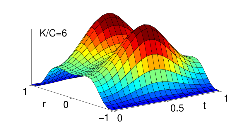
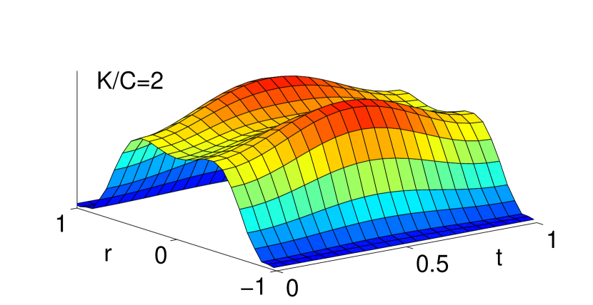
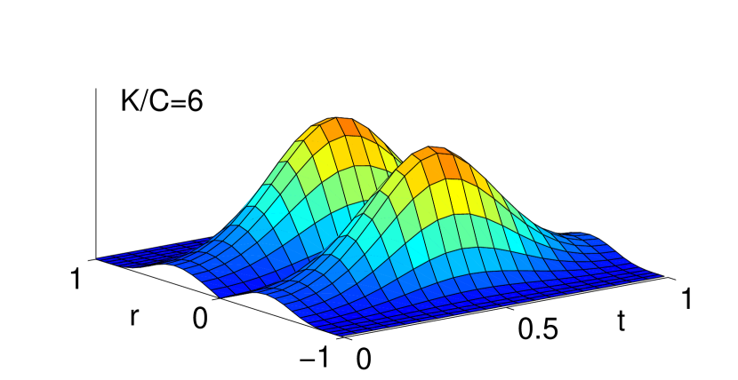
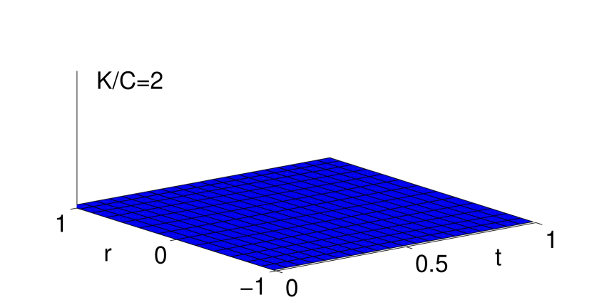
Figure 10: Lumps in $|F_{s\bar{s}}|$ for various values of $K$ in the ‘zeroes together’ solution (left) and ‘zeroes apart’ (right) for $C=1$, $\beta=2\pi$, using the same vertical scale throughout. The positions of the lumps should be compared with the positions of the zeroes of $\text{det}(\Phi)$, as indicated in figs 8 and 9. It should also be noted that the lumps are of different sign in each case.

5 SU(3) Periodic Monopoles

Monopoles in $\mathbb{R}^{3}$ have been considered for higher rank gauge groups by various authors [9, 25, 26, 27]. In this section we apply the results of the spectral approximation to the SU(3) periodic monopole and consider the basic properties for $\bm{k}=(1,1)$ and $\bm{k}=(2,1)$, which have two and four reduced relative moduli, respectively.

Following the arguments of section 1.1, the SU(3) periodic monopole has spectral curve (12)

$$w^{3}+P_{1,k_{1}}(\zeta)w^{2}+P_{2,k_{2}}(\zeta)w-1\,=\,0\qquad\text{where}\qquad P_{i,k_{i}}(\zeta)\,=\,a_{i,k_{i}}\zeta^{k_{i}}+\ldots+a_{i,1}\zeta+a_{i,0}.$$

As discussed in sections 1.1 and 1.3, we take $k_{1}\geq k_{2}$. The root diagram was shown in fig. 1. Our procedure will be to express the coefficients of $P_{i,k_{i}}(\zeta)$ in terms of the boundary data (3, 7) and hence to determine the positions of spectral points from the discriminant $\mathcal{D}_{(k_{1},k_{2})}$. In analogy with section 2.1, we are interested in the eigenvalues of the holonomy $V$. This manipulation is performed numerically to give three eigenvalues $w_{i}=\text{exp}(\beta(r_{i}+\text{i}t_{i}))$ from which $\hat{\Phi}\propto\text{diag}(r_{1},r_{2},r_{3})$ and the quantities of interest are

$$\mathcal{E}\,\propto\,\nabla^{2}\left(r_{1}^{2}+r_{2}^{2}+r_{3}^{2}\right),\qquad\qquad\text{discriminant}\,=\,(r_{1}-r_{2})^{2}(r_{2}-r_{3})^{2}(r_{3}-r_{1})^{2}.$$

5.1 Trivial Embedding

The $\bm{k}=(1,1)$ spectral curve has coefficients

$$\bm{k}\,=\,(1,1)\qquad\left\{\begin{array}[]{c c c}a_{1,1}\,=\,-\text{e}^{\mathfrak{v}_{1}}&&a_{1,0}\,=\,-(\mu_{1}\text{e}^{\mathfrak{v}_{1}}+\text{e}^{\mathfrak{v}_{2}})\\ a_{2,1}\,=\,\text{e}^{\mathfrak{v}_{1}+\mathfrak{v}_{2}}&&a_{2,0}\,=\,(\mu_{1}+\mu_{2})\text{e}^{\mathfrak{v}_{1}+\mathfrak{v}_{2}}+\text{e}^{-\mathfrak{v}_{2}},\end{array}\right.$$ (31)

and discriminant

$$\mathcal{D}_{(1,1)}\,=\,a_{1,1}^{2}a_{2,1}^{2}\zeta^{4}+2\left(a_{1,1}a_{2,1}(a_{1,1}a_{2,0}+a_{1,0}a_{2,1})+2(a_{1,1}^{3}-a_{2,1}^{3})\right)\zeta^{3}+\ldots,$$

such that the spectral points are centered if the $\zeta^{3}$ term vanishes,

$$(2\mu_{1}+\mu_{2})\text{e}^{\mathfrak{v}_{1}+2\mathfrak{v}_{2}}\,=\,\text{e}^{3\mathfrak{v}_{2}}+1.$$

As noted in section 1.3, the fact $K$ is repeated means the Nahm data will have a singularity at finite $|r|$. As we are working with SU(3) the determinant will have three zeroes.

If $\mathfrak{v}_{2}=0$ and $\mu_{2}=0$ (such that the centering condition becomes $\mu_{1}\text{e}^{\mathfrak{v}_{1}}=1$) the monopole is an SU(2) monopole embedded along the root $\bm{\beta}_{3}^{\ast}=-\bm{\beta}_{1}^{\ast}-\bm{\beta}_{2}^{\ast}$. This allows the spectral curve to be factorised,

$$(w-1)\left(w^{2}-(\text{e}^{\mathfrak{v}_{1}}\zeta+1)w+1\right)\,=\,0.$$

In this limit, three of the spectral points coincide and, as expected, the monopole fields resemble those of an SU(2) monopole with $\bm{k}=(1)$.

$\underline{\mathfrak{v}_{2}\neq 0}$

We deform away from the SU(2) embedding by changing the boundary conditions to allow non-zero $\mathfrak{v}_{2}$. The spectral curve again factorises, and centering identifies

$$a_{1,0}\,=\,-\tfrac{1}{2}\left(3\text{e}^{\mathfrak{v}_{2}}+\text{e}^{-2\mathfrak{v}_{2}}\right)\qquad\qquad a_{2,0}\,=\,\tfrac{1}{2}\left(\text{e}^{2\mathfrak{v}_{2}}+3\text{e}^{-\mathfrak{v}_{2}}\right).$$

with $a_{1,1}$ and $a_{2,1}$ as in (31). The situation is shown in fig. 11. In the Nahm picture, the Higgs field has a simple pole at $s=\mathfrak{v}_{2}/\beta$. For $\mu_{2}=0$ one of the zeroes coincides with the pole, giving the two zeroes characteristic of SU(2) solutions.

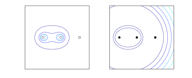
Figure 11: Deformations of the $\bm{k}=(1,1)$ monopole by changing $\mathfrak{v}_{2}$ away from zero. Here $\mathfrak{v}_{2}=1.2$. On the left is plotted the energy density and on the right the discriminant of $\hat{\Phi}$. There is no energy density associated with the coincident spectral points on the right. The discriminant vanishes on a line joining the spectral points on the left, and on a circle passing through the double spectral point and surrounding the other two.

$\underline{\mu_{2}\neq 0}$

In a similar way, we can fix the boundary conditions to $\mathfrak{v}_{2}=0$ and allow the moduli $\mu_{1}$ and $\mu_{2}$ to vary in such a way that the spectral points remain centered. The coefficients in (31) become

$$a_{1,1}\,=\,-\text{e}^{\mathfrak{v}_{1}}\qquad\qquad a_{1,0}\,=\,-(1+\mu_{1}\text{e}^{\mathfrak{v}_{1}})\qquad\qquad a_{2,1}\,=\,\text{e}^{\mathfrak{v}_{1}}\qquad\qquad a_{2,0}\,=\,3-\mu_{1}\text{e}^{\mathfrak{v}_{1}}.$$

Varying $\mu_{1}$ separates the three coincident spectral points and introduces a second fundamental monopole, as shown in fig. 12.

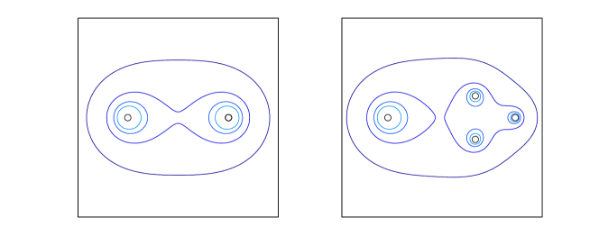
Figure 12: Deformations of the $\bm{k}=(1,1)$ monopole with $\mathfrak{v}_{2}=0$. On the left are contours of energy density for $\mu_{1}\text{e}^{\mathfrak{v}_{1}}=1$. On the right, for $\mu_{1}\text{e}^{\mathfrak{v}_{1}}=1.2$. For these examples, the discriminant pairs up the spectral points on the horizontal axis. The line of zero discriminant joining the other two points is found to wrap around the left hand spectral point.

5.2 Minimal Symmetry Breaking

The $\bm{k}=(2,1)$ spectral curve has

$$\bm{k}\,=\,(2,1)\qquad\left\{\begin{array}[]{c c c}a_{1,2}\,=\,-\text{e}^{\mathfrak{v}_{1}}&&a_{1,1}\,=\,-\mu_{1}\text{e}^{\mathfrak{v}_{1}}\\ a_{2,1}\,=\,\text{e}^{\mathfrak{v}_{1}+\mathfrak{v}_{2}}+\text{e}^{-\mathfrak{v}_{2}}&&a_{2,0}\,=\,(\mu_{1}+\mu_{2})\text{e}^{\mathfrak{v}_{1}+\mathfrak{v}_{2}}-\mu_{2}\text{e}^{-\mathfrak{v}_{2}},\end{array}\right.$$

and discriminant

$$\mathcal{D}_{(2,1)}\,=\,a_{1,2}^{2}\left(a_{2,1}^{2}+4a_{1,2}\right)\zeta^{6}+2a_{1,2}\left(a_{1,2}a_{2,1}a_{2,0}+a_{1,1}a_{2,1}^{2}+6a_{1,1}a_{1,2}\right)\zeta^{5}+\ldots$$

and the remaining coefficient, $a_{1,0}$, is to be considered a modulus. In this case, two of the $\ell_{i}$ are repeated, allowing minimal symmetry breaking if $\bm{\mathfrak{v}}=(2\mathfrak{v},-\mathfrak{v},-\mathfrak{v})$, for which centering implies that

$$a_{1,2}\,=\,-\text{e}^{2\mathfrak{v}}\qquad\qquad a_{1,1}\,=\,-\mu_{1}\text{e}^{2\mathfrak{v}}\qquad\qquad a_{2,1}\,=\,2\text{e}^{\mathfrak{v}}\qquad\qquad a_{2,0}\,=\,\mu_{1}\text{e}^{\mathfrak{v}}.$$

In fact, this condition is equivalent to the coefficient of $\zeta^{6}$ in $\mathcal{D}_{(2,1)}$ vanishing, which was not a possibility for the SU(2) or $\bm{k}=(1,1)$ cases considered so far. The coefficient of $\zeta^{4}$ also vanishes if we set $P_{1,2}=-\frac{1}{4}P_{2,1}^{2}$, such that three of the spectral points are sent to infinity. This leaves $\mu_{1}$ as a complex modulus, and a symmetric configuration is obtained by taking $\mu_{1}=0$, such that the coefficients of $\zeta^{2}$ and $\zeta$ also vanish, fig. 13.

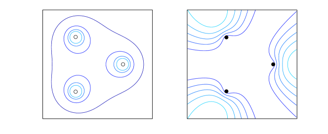
Figure 13: $\mathbb{Z}_{3}$-symmetric $\bm{k}=(2,1)$ periodic monopole with spectral curve $w^{3}-\zeta^{2}w^{2}+2\zeta w-1=0$. Energy density on the left and the discriminant of $\hat{\Phi}$ on the right.

$\underline{\mathfrak{v}_{2}\neq\mathfrak{v}_{3}}$

Following [10] we deform by adding to $\bm{\mathfrak{v}}$ a constant diagonal term $\delta\bm{\beta}_{2}^{\ast}$ for some complex $\delta$ (we can rearrange the entries such that $\Re(\delta)\geq 0$), fig. 14. The total energy (5) is unchanged, but there is a different pattern of symmetry breaking. Explicitly, $a_{1,2}$ and $a_{1,1}$ are unaltered, while

$$a_{2,1}\,=\,2\text{e}^{\mathfrak{v}}\cosh(\delta)\qquad\qquad a_{2,0}\,=\,\text{e}^{\mathfrak{v}}\left(\mu_{1}\text{e}^{\delta}+2\mu_{2}\sinh(\delta)\right).$$

Such deformations have the effect of moving the three remaining spectral points in from infinity. A particularly symmetric example, with $\delta=\text{i}\pi/2$, is shown in fig. 15.

Figure 14: Deformation of the subleading term. Starting from the shaded point we deform parallel to $\bm{\beta}_{2}^{\ast}$.

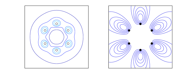
Figure 15: $\mathbb{Z}_{6}$-symmetric $\bm{k}=(2,1)$ periodic monopole with spectral curve $w^{3}-\zeta^{2}w^{2}-1=0$. On the left is plotted the energy density and on the right the discriminant of $\hat{\Phi}$.

The $\bm{k}=(2,1)$ Nahm data is of rank $2$, smooth, and has three zeroes. For the spectral curve $w^{3}-\zeta^{2}w^{2}+2a\zeta w-1=0$ relevant to both the cases considered above, the Hitchin Higgs fields have

$$\text{tr}(\Phi)\,=\,2aw^{-1}\qquad\qquad-\text{det}(\Phi)\,=\,w-w^{-2}.$$

The determinant has zeroes at $\beta s=0,\pm 2\text{i}\pi/3$. This is reminiscent of the fact that the most symmetric $\bm{k}=(2)$ configurations were found to have zeroes located symmetrically on the Hitchin cylinder (fig. 8).

5.3 Speculative Geodesic

In section 4.2 it was shown that of the four real relative moduli of the SU(2) monopole of charge $\bm{k}=(2)$, there was a two dimensional geodesic submanifold corresponding to varying the two moduli present in the spectral curve. This justified the deduction of one dimensional submanifolds in section 3.3. The SU(3) monopole of charge $\bm{k}=(1,1)$ also has four real relative moduli, and we will assume that the two which appear in the spectral curve again provide a geodesic submanifold.

The reduced moduli are constrained by looking for configurations invariant under a reflection in the $x$-axis, which we perform by mapping $\zeta\mapsto\bar{\zeta}$ and $w\mapsto\bar{w}$. This requires all the coefficients $a_{i,j}$ in (31) to be real. A symmetric choice of boundary conditions is provided by requiring the two fundamental monopoles to be of the same size, which we do by further imposing invariance of the spectral curve under $\zeta\mapsto-\zeta$ and $w\mapsto w^{-1}$, resulting in

$$a_{1,1}\,=\,-\text{e}^{\mathfrak{v}_{1}}\qquad a_{1,0}\,=\,1-\mu_{1}\text{e}^{\mathfrak{v}_{1}}\qquad a_{2,1}\,=\,-\text{e}^{\mathfrak{v}_{1}}\qquad a_{2,0}\,=\,\mu_{1}\text{e}^{\mathfrak{v}_{1}}-1,$$

where $\mathfrak{v}_{1}$ is fixed and $\mu_{1}\in\mathbb{R}$ provides a one parameter family (note this is a different situation from that of section 5.1, where $\mathfrak{v}_{2}=0$). Fig. 16

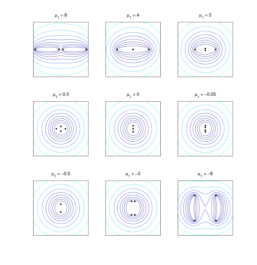
Figure 16: Sequence arising by varying the real parameter $\mu_{1}$ with $\mathfrak{v}_{1}=0$ and $\mathfrak{v}_{2}=\text{i}\pi$. Plots show the discriminant of $\hat{\Phi}$. In the Nahm transformed picture, motion of the zeroes of $\text{det}(\Phi)$ follows a similar pattern to that shown in fig. 8, though now with the third zero fixed at $s=0$ and the singularity at $s=\text{i}\pi/\beta$. The zeroes are coincident when $\mu_{1}=4$ and two of them reach the singularity when $\mu_{1}=0$.

illustrates the resulting scattering process. As mentioned in [9], the monopoles scatter back off each other in a head-on collision, though with a deformed shape. By allowing different boundary conditions, one can in fact find one parameter families describing the less symmetric cases where one monopole is larger than the other, or when one of the incoming monopoles is rotated by an angle of $\pi/2$. As was noted for the SU(2) periodic monopole in sections 2.2 and 3.3, we find that when the spectral points are well separated those of each fundamental monopole are joined by lines of zero discriminant.

6 Dirac Singularities and the Doubly Periodic Instanton

In the region where $z$ dependence can be ignored, the fields of a configuration of positive and negative Dirac monopoles at $\zeta=\zeta_{i}^{\pm}$ are

$$\text{i}\beta\hat{\Phi}\,=\,\frac{1}{2}\sum_{i=1}^{n_{+}}\log\left(|\zeta-\zeta_{i}^{+}|^{2}\right)-\frac{1}{2}\sum_{i=1}^{n_{-}}\log\left(|\zeta-\zeta_{i}^{-}|^{2}\right)$$

$$\text{i}\beta\hat{A}_{z}\,=\,\frac{\text{i}}{2}\sum_{i=1}^{n_{+}}\log\left(\frac{\bar{\zeta}-\bar{\zeta}_{i}^{+}}{\zeta-\zeta_{i}^{+}}\right)-\frac{\text{i}}{2}\sum_{i=1}^{n_{-}}\log\left(\frac{\bar{\zeta}-\bar{\zeta}_{i}^{-}}{\zeta-\zeta_{i}^{-}}\right)$$

allowing us to compute the holonomy and hence write down the spectral curve,

$$\left(\prod_{i=1}^{n_{-}}(\zeta-\zeta_{i}^{-})\right)\,w-\left(\prod_{i=1}^{n_{+}}(\zeta-\zeta_{i}^{+})\right)\,=\,0,$$ (32)

and there are thus no moduli. Cherkis & Kapustin [3] argue that singularities can be introduced to the periodic monopole by modifying the spectral curve (12) to

$$P_{0,n_{-}}(\zeta)w^{N}+P_{1,k_{1}}(\zeta)w^{N-1}+\ldots+P_{N-1,k_{N-1}}(\zeta)w+(-1)^{N}P_{N,n_{+}}(\zeta)\,=\,0$$

where $P_{0,n_{-}}(\zeta)$ and $P_{N,n_{+}}(\zeta)$ are the monic polynomials appearing in (32).

The principal use of Dirac singularities is in changing the boundary conditions on the Hitchin data. In particular, adding $K$ positive and $K$ negative singularities to the monopole with $\bm{k}=(K,K,\ldots,K)$ renders $\text{det}(\Phi)$ smooth at $|r|\to\infty$, albeit with singularities at finite $|r|$ due to $K$ appearing more than once. We illustrate this by looking at the SU(2) monopole with two singularities, where we require the spectral curve to be invariant under $w\mapsto w^{-1}$ in order that the monopole fields are valued in $\mathfrak{su}(2)$. The relevant spectral curve is

$$(\zeta-\zeta_{0})w^{2}-2(a\zeta+b)w+(\zeta-\zeta_{0})\,=\,0$$ (33)

such that the boundary conditions (7) translate to

$$a\,=\,\cosh(\mathfrak{v})\qquad\qquad b\,=\,\mu\sinh(\mathfrak{v})-\zeta_{0}\cosh(\mathfrak{v})$$

and the spectral curve (33) can be rearranged to give the Hitchin Higgs field

$$\Phi\,=\,\zeta\,=\,\zeta_{0}+\frac{\mu\sinh(\mathfrak{v})}{\cosh(\beta s)-\cosh(\mathfrak{v})}.$$ (34)

Applying the method of section 2, spectral points are located at

$$\zeta\,=\,\frac{\zeta_{0}+b}{1-a}\qquad\text{and}\qquad\zeta\,=\,\frac{\zeta_{0}-b}{1+a},$$

which are centered if $ab+\zeta_{0}=0$, and are coincident if $a\zeta_{0}+b=0$. The monopole Higgs field is

$$\hat{\Phi}\,=\,\frac{\text{i}}{\beta}\,\Re\cosh^{-1}\left(\cosh(\mathfrak{v})+\frac{\mu\sinh(\mathfrak{v})}{\zeta-\zeta_{0}}\right)\sigma_{3}.$$

In the case where $a=0$, $\text{i}b=C$, this simplifies to

$$\hat{\Phi}\,=\,\frac{\text{i}}{\beta}\,\Re\cosh^{-1}\left(\frac{C}{\zeta}\right)\sigma_{3}$$

which is related to the fields of sections 2.1 and 2.2 by a simple inversion transformation $\zeta\mapsto C^{2}/\bar{\zeta}$, with a corresponding change of boundary conditions.

In analogy with monopoles appearing as constituents of periodic instantons (see, for example, [28, 29, 11]), it is expected that the doubly periodic instanton will be related to the periodic monopole [3, 7]. The Nahm data for the doubly periodic instanton are Hitchin equations on a 2-torus $T^{2}$. The charge 1 case is considered by [7], where the Hitchin system is Abelian. This allows the Hitchin gauge potentials to be expressed as derivatives of a harmonic potential, and the Higgs field is chosen to be proportional to $A_{s}$ in order to share the same singularities,

$$A_{s}\,=\,\partial_{s}\varphi\qquad\qquad A_{\bar{s}}\,=\,-\partial_{\bar{s}}\varphi\qquad\qquad\Phi\,=\,\zeta_{0}+\alpha\partial_{s}\varphi$$

where, in our notation, the fundamental solution to Laplace’s equation on the torus is

$$\varphi\,=\,\frac{1}{2}\,\log\frac{\left|\vartheta_{3}\left(\tfrac{\text{i}}{2\pi}(\bar{s}\beta_{1}+\bar{\mathfrak{v}})+\tfrac{1}{2}+\tfrac{\text{i}\beta_{1}}{2\beta_{2}},\tfrac{\text{i}\beta_{1}}{\beta_{2}}\right)\right|^{2}}{\left|\vartheta_{3}\left(\tfrac{\text{i}}{2\pi}(\bar{s}\beta_{1}-\bar{\mathfrak{v}})+\tfrac{1}{2}+\tfrac{\text{i}\beta_{1}}{2\beta_{2}},\tfrac{\text{i}\beta_{1}}{\beta_{2}}\right)\right|^{2}}$$

with $\beta_{1}$ and $\beta_{2}$ the periods of the instanton, and $\vartheta_{3}$ is the doubly periodic Jacobi theta-function, which is conveniently expressed as

$$\vartheta_{3}(w,\tau)\,=\,\sum_{n=-\infty}^{\infty}\text{e}^{\text{i}\pi n^{2}\tau+2\text{i}\pi nw}.$$ (35)

The result (34) is recovered in the limit $\beta_{1}=\beta$, $\beta_{2}\to 0$, such that only the $n=0$ and $n=-1$ terms contribute to (35),

$$\varphi\,=\,\frac{1}{2}\,\log\frac{\left|1-\text{e}^{\beta\bar{s}+\bar{\mathfrak{v}}}\right|^{2}}{\left|1-\text{e}^{\beta\bar{s}-\bar{\mathfrak{v}}}\right|^{2}}\qquad\Rightarrow\qquad\Phi\,=\,\zeta_{0}-\frac{\alpha\beta}{2}\frac{\sinh(\mathfrak{v})}{\cosh(\beta s)-\cosh(\mathfrak{v})},$$

which is precisely of the form (34). In [7], $\alpha$ is interpreted as a size, which when set to zero provides axially symmetric fields. In the monopole picture this corresponds to setting $\mu=0$, in which case $a\zeta_{0}+b=0$ and the spectral points coincide, again leading to axial symmetry.

The need for singularities when making the comparison with the doubly periodic instanton is brought about by a change in the boundary conditions, and is reminiscent of the intepretation of periodic instantons as monopoles whose gauge group is a loop group [8]. In practice, this amounts to adding a root to the gauge group such that all of the $\ell_{i}$ vanish and we are at the origin of the root diagram, fig. 1. From the discussion of sections 1 and 2, the additional fundamental monopole expected from the extra root fits in with the observation in [7] that the doubly periodic instanton consists of two periodic monopole constituents, separated in one of the periodic directions. It would be interesting to explore this result further, although this would require a departure from the approximation presented in this paper.

7 Concluding Remarks

In this paper we developed a technique, motivated by [1, 3, 4, 5], to study the singly periodic BPS monopole. This was checked against numerical studies of the SU(2) cases of charge $1$ and $2$. Geodesic motion on an effective two dimensional moduli space compared favourably with analytic results for charge $2$. In particular, it was found that motion transverse to the periodic direction provides a geodesic submanifold. Some simple SU(3) configurations and singular periodic monopoles were also considered in this context. The Nahm transform relates the periodic monopole to a Hitchin system on the cylinder, giving rise to lumps whose motion is described, at large separations, by the motion of zeroes of the spectral curve polynomial.

Short of finding explicit solutions for the monopole fields or the moduli space metric, some unanswered questions which will provide the basis for future work include whether the two energy peaks associated to each fundamental monopole can be understood as ‘constituents’ in their own right. This has been done for the periodic instanton, which was reconstructed by [11] in terms of the Nahm data of its monopole constituents. It would also be of interest to study explicitly the limits of the periodic monopole for large and small periods. Preliminary numerical work indicates the Nahm data behaves as hoped (see section 4.3). As a step in this direction, a study of how the moduli describing a phase difference and $z$ separation appear in the Nahm dual picture will be presented in [22].

Appendix A Symmetries of the Nahm Operator

In this appendix we explain in detail the procedure followed in section 4.2, with reference to the example of the $K\in\mathbb{R}$ geodesic of the ‘zeroes together’ solution.

The map $(s;K)\mapsto(\bar{s};\bar{K})$ transforms $(r,t)\mapsto(r,-t)$,

$$\mu_{+}(s;K)\,=C\cosh(\beta s)+K/2\,\mapsto\,C\cosh(\beta\bar{s})+\bar{K}/2\,=\,\bar{\mu}_{+}(s;K)$$

and

$$\mu_{-}(s;K)\,=\,1\,\mapsto\,\bar{\mu}_{-}(s;K).$$

Equation (28) is invariant, so $\Re(\psi)(s;K)\mapsto\Re(\psi)(s;K)$. Recalling that in this case $\Im(\psi)=0$ gives the transformation of $a$,

$$a(s;K)\,=\,-\tfrac{1}{8}(\partial_{r}+\text{i}\partial_{t})\psi\,\mapsto\,-\tfrac{1}{8}(\partial_{r}-\text{i}\partial_{t})\psi\,=\,\bar{a}(s;K).$$

Combining these results we obtain the transformed Hitchin fields (27),

$$\Phi(s;K)\,=\begin{pmatrix}0&\mu_{+}\text{e}^{\psi/2}\\ \mu_{-}\text{e}^{-\psi/2}&0\end{pmatrix}(s;K)\mapsto\,\Phi^{\prime}(s^{\prime};K^{\prime})\,=\,\begin{pmatrix}0&\bar{\mu}_{+}\text{e}^{\psi/2}\\ \bar{\mu}_{-}\text{e}^{-\psi/2}&0\end{pmatrix}(s;K),$$

$$A_{\bar{s}}(s;K)\,=\,a(s;K)\sigma_{3}\,\mapsto\,A_{\bar{s}}^{\prime}(s^{\prime};K^{\prime})\,=\,\bar{a}(s;K)\sigma_{3}\,=\,-A_{s}(s;K)$$

$$A_{s}(s;K)\,=\,-\bar{a}(s;K)\sigma_{3}\,\mapsto\,A_{s}^{\prime}(s^{\prime};K^{\prime})\,=\,-a(s;K)\sigma_{3}\,=\,-A_{\bar{s}}(s;K).$$

The Nahm operator $\Delta$ constructed from the new fields is

$$\Delta^{\prime}\,=\,\begin{pmatrix}\bm{1}_{2}\otimes(2\partial_{s}-z)-2A_{s}&\bm{1}_{2}\otimes\zeta-(\Phi^{\prime})^{\dagger}\\ \bm{1}_{2}\otimes\bar{\zeta}-\Phi^{\prime}&\bm{1}_{2}\otimes(2\partial_{\bar{s}}+z)-2A_{\bar{s}}\end{pmatrix}.$$

Noting that $\Phi^{\prime}$ can be written in terms of $\Phi$ as $\Phi^{\prime}=\sigma_{1}\Phi^{\dagger}\sigma_{1}$, the new Nahm operator $\Delta^{\prime}$ can be obtained from the original one (30) by the combined transformation

$$\Delta^{\prime}\,=\,U^{-1}\Delta U\qquad\qquad(\zeta,z)\,\mapsto\,(\bar{\zeta},-z)$$

with $U=\sigma_{1}\otimes\sigma_{1}$. Consequently, $\Psi$ transforms as

$$\Psi_{\pm}\,\mapsto\,\sigma_{1}\Psi_{\mp}$$

such that the new monopole fields evaluated at $(\bar{\zeta},-z)$ are the same as the old ones at $(\zeta,z)$. A monopole configuration symmetric under $(\zeta,z)\mapsto(\bar{\zeta},-z)$ is thus invariant under $K\mapsto\bar{K}$, and leaves us with the one parameter family of solutions described by $\Im(K)=0$.

References

- [1] S. Cherkis, A. Kapustin, Nahm Transform for Periodic Monopoles and =2 Super Yang-Mills Theory, Commun. Math. Phys. 218 (2001) 333, arXiv:hep-th/0006050
- [2] S. A. Cherkis, A. Kapustin, Hyper-Kähler metrics from periodic monopoles, Phys. Rev. D 65 (2002) 084015, arXiv:hep-th/0109141
- [3] S. A. Cherkis, A. Kapustin, Periodic Monopoles With Singularities And =2 Super-QCD, Commun. Math. Phys. 234 (2003) 1-35, arXiv:hep-th/0011081
- [4] R. S. Ward, Periodic monopoles, Phys. Lett. B 619 (2005) 177, arXiv:hep-th/0505254
- [5] D. Harland, R. S. Ward, Dynamics of periodic monopoles, Phys. Lett. B 675 (2009) 262, arXiv:0901.4428 [hep-th]
- [6] M. Jardim, A survey on Nahm transform, J. Geom. Phys. 52 (2004) 313, arXiv:math/0309305 [math.DG]
- [7] C. Ford, J. M. Pawlowski, Doubly periodic instantons and their constituents, Phys. Rev. D 69 (2004) 065006, arXiv:hep-th/0302117
- [8] D. Harland, Chains of Solitons, PhD thesis, University of Durham (2008), etheses.dur.ac.uk/2303/
- [9] N. Manton, P. Sutcliffe, Topological Solitons, CUP (2007)
- [10] R. S. Ward, Deformations of the Embedding of the SU(2) Monopole Solution in SU(3), Commun. Math. Phys. 86 (1982) 437
- [11] K. Lee, C. Lu, SU(2) calorons and magnetic monopoles, Phys. Rev. D 58 (1998) 025011
- [12] P. J. Braam, P. van Baal, Nahm’s Transformation for Instantons, Commun. Math. Phys. 122 (1989) 267
- [13] E. Corrigan, P. Goddard, Construction of Instanton and Monopole Solutions and Reciprocity, Ann. Phys. 154 (1984) 253
- [14] N. J. Hitchin, The Self-Duality Equations on a Riemann Surface, Proc. Lond. Math. Soc. (3) 55 (1987) 59
- [15] A. Kapustin, Solution of N=2 gauge theories via compactification to three dimensions, Nucl. Phys. B 534 (1998) 531, arXiv:hep-th/9804069
- [16] R. S. Ward, A Yang-Mills-Higgs Monopole of Charge 2, Commun. Math. Phys. 79 (1981) 317
- [17] G. V. Dunne, V. Khemani, Numerical investigation of monopole chains, J. Phys. A 38 (2005) 9359
- [18] D. Harland, private communication
- [19] I. S. Gradshteyn, I. M. Ryzhik, A. Jeffrey (ed.), Table of Integrals, Series, and Products, Academic Press (1994), equations (3.617), (6.141), (6.142), (8.111)-(8.113), (8.126), (9.100)
- [20] S. Bolognesi, Multi-monopoles and magnetic bags, Nucl. Phys. B 752 (2006) 93, arXiv:hep-th/0512133
- [21] G. W. Gibbons, S. W. Hawking, Gravitational Multi-Instantons, Phys. Lett. B 78 (1978) 430
- [22] R. Maldonado, R. S. Ward, Geometry of periodic monopoles, Phys. Rev. D 88 (2013) 125013, arXiv:1309.7013 [hep-th]
- [23] R. Maldonado, Higher charge periodic monopoles, arXiv:1311.6354 [hep-th]
- [24] R. Maldonado, Periodic Monopoles, PhD thesis, University of Durham (2014), etheses.dur.ac.uk/10729/
- [25] E. J. Weinberg, Fundamental Monopoles and Multimonopole Solutions for Arbitrary Simple Gauge Groups, Nucl. Phys. B 167 (1980) 500
- [26] K. Lee, E. J. Weinberg, P. Yi, Moduli space of many BPS monopoles for arbitrary gauge groups, Phys. Rev. D 54 (1996) 1633
- [27] Ya. Shnir, SU(N) monopoles with and without SUSY, arXiv:hep-th/0508210
- [28] T. C. Kraan, P. van Baal, Periodic instantons with non-trivial holonomy, Nucl. Phys. B 533 (1998) 627, arXiv:hep-th/9805168
- [29] T. C. Kraan, P. van Baal, Monopole constituents inside SU(n) calorons, Phys. Lett. B 435 (1998) 389, arXiv:hep-th/9806034