Stability of eigenvalues of quantum graphs with respect to magnetic perturbation and the nodal count of the eigenfunctions

Abstract.

We prove an analogue of the magnetic nodal theorem on quantum graphs: the number of zeros $\phi$ of the $n$-th eigenfunction of the Schrödinger operator on a quantum graph is related to the stability of the $n$-th eigenvalue of the perturbation of the operator by magnetic potential. More precisely, we consider the $n$-th eigenvalue as a function of the magnetic perturbation and show that its Morse index at zero magnetic field is equal to $\phi-(n-1)$.

1. Introduction

A quantum graph is a metric graph equipped with a self-adjoint differential “Hamiltonian” operator (usually of Schrödinger type) defined on the edges and matching conditions specified at the vertices. Graph models in general, and quantum graphs in particular, have long been used as a simpler setting to study complicated phenomena. We refer the interested reader to the reviews [1, 2, 3], collections of papers [4, 5], and the recent monograph [6] for an introduction to quantum graphs and their applications.

Quantum graphs have been especially fruitful models for studying the properties of zeros of the eigenfunctions [7, 8]. Of particular interest is the relationship between the sequential number of the eigenfunction and the number of its zeros, which we will refer to as the nodal point count. It was on quantum graphs that the relationship between the stability of the nodal partition of an eigenfunction and its nodal deficiency was first discussed [9]. Since then, the result has been extended to discrete graphs [10] and bounded domains in $\mathbb{R}^{d}$ [11].

In a similar-spirited development, it has been discovered that the nodal point count on discrete graphs is connected to the stability of the eigenvalue with respect to a perturbation by a magnetic field [12] (see also [13] for an alternative proof). While the magnetic result drew inspiration from the developments for nodal partitions, the relationship between the two results was very implicit in the original proof [12] and was not at all relevant in the proof of [13].

The purpose of the current paper is three-fold. We prove an analogue of the magnetic theorem of [12] on quantum graphs. This is done by establishing a clear and explicit link between magnetic perturbation and the perturbation of the nodal partition. Along the way, we remove some superfluous (and troublesome) assumptions from the nodal partitions theorem of [9].

A proof of the magnetic theorem on the simplest of quantum graphs, a circle, has already been found in [13]. This proof uses the explicitly available nodal point count and thus is impossible to generalize to any non-trivial graph. However, we do acknowledge drawing inspiration (in particular, in the use of Wronskian) from the work of [13].

Finally, we would like to mention that the main result of the present paper has already been used by R. Band to prove an elegant “inverse nodal theorem” on quantum graphs [14], which appears in this same volume.

2. Main results

We start by defining the quantum graph, following the notational conventions of [6]. We also refer the reader to [6] for the proofs of all background results used in this section.

Let $\Gamma$ be a compact metric graph with vertex set $V$ and edge set $E$. Let $\widetilde{H}^{k}(\Gamma,\mathbb{C})$ be the space of all complex-valued functions that are in the Sobolev space $H^{k}(e)$ for each edge, or in other words

$$\widetilde{H}^{k}(\Gamma,\mathbb{C})=\oplus_{e\in E}H^{k}(e),$$

while $\widetilde{H}^{k}(\Gamma,\mathbb{R})$ will denote the space of all real-valued functions that are in the Sobolev space $H^{k}(e)$ for each edge. We define $\widetilde{L}^{k}(\Gamma,\mathbb{C})$ and $\widetilde{L}^{k}(\Gamma,\mathbb{R})$ similarly. Consider the Schrödinger operator with electric potential $q:\Gamma\rightarrow\mathbb{R}$ defined by

$$H^{0}:f\mapsto-\frac{d^{2}f}{dx^{2}}+qf,$$

acting on the functions from $\widetilde{H}^{2}(\Gamma,\mathbb{C})$ satisfying the $\delta$-type boundary conditions

(1) $$\left\{\begin{array}[]{l}f(x)\mbox{ is continuous at v},\\ \sum_{e\in{E_{v}}}\frac{df}{dx_{e}}(v)=\chi_{v}f(v),\qquad\chi_{v}\in\mathbb{R}.\end{array}\right.$$

Here the potential $q(x)$ is assumed to be piecewise continuous. The set $E_{v}$ is the set of edges joined at the vertex $v$; by convention, each derivative at a vertex is taken into the corresponding edge. We denote by $x_{e}$ the local coordinate on edge $e$.

On vertices of degree one, we also allow the Dirichlet condition $f(v)=0$, which is formally equivalent to $\chi_{v}=\infty$. In this case, we do not count the Dirichlet vertex as a zero, neither when specifying restrictions on the eigenfunction nor when counting its zeros.

The operator $H^{0}$ is self-adjoint, bounded from below, and has a discrete set of eigenvalues that can be ordered as

$$\lambda_{1}\leq\lambda_{2}\leq\ldots\leq\lambda_{n}\leq\ldots\hskip 7.22743pt.$$

The magnetic Schrödinger operator on $\Gamma$ is given by

$$H^{A}(\Gamma):f\mapsto-\left(\frac{d}{dx}-iA(x)\right)^{2}f+qf,\qquad f\in\widetilde{H}^{2}(\Gamma,\mathbb{C}),$$

where the one-form $A(x)$ is the magnetic potential (namely, the sign of $A(x)$ changes with the orientation of the edge). The $\delta$-type boundary conditions are now modified to

$$\left\{\begin{array}[]{l}f(x)\mbox{ is continuous at v},\\ \sum_{e\in{E_{v}}}\left(\frac{df}{dx_{e}}(v)-iA(v)f(v)\right)=\chi_{v}f(v),\qquad\chi_{v}\in\mathbb{R}.\end{array}\right.$$

Let $\beta=|E|-|V|+1$ be the first Betti number of the graph $\Gamma$, i.e. the rank of the fundamental group of the graph. Informally speaking, $\beta$ is the number of “independent” cycles on the graph. Up to a change of gauge, a magnetic field on a graph is fully specified by $\beta$ fluxes $\alpha_{1},\alpha_{2},\ldots,\alpha_{\beta}$, defined as

$$\alpha_{j}=\oint_{\sigma_{j}}A(x)dx\mod 2\pi,$$

where $\{\sigma_{j}\}$ is a set of generators of the fundamental group. In other words, magnetic Schrödinger operators with different magnetic potentials $A(x)$, but the same fluxes $(\alpha_{1},\ldots,\alpha_{\beta})$, are unitarily equivalent. Therefore, the eigenvalues $\lambda_{n}(H^{A})$ can be viewed as functions of $\boldsymbol{\alpha}=(\alpha_{1},\ldots,\alpha_{\beta})$.

In this paper, we will prove the following main result:

Theorem 1.

Let $\psi$ be the eigenfunction of $H^{0}$ that corresponds to a simple eigenvalue $\lambda=\lambda_{n}(H^{0})$. We assume that $\psi$ is non-zero on vertices of the graph. We denote by $\phi$ the number of internal zeros of $\psi$ on $\Gamma$.

Consider the perturbation $H^{A}$ of the operator $H^{0}$ by a magnetic field $A$ with fluxes $\boldsymbol{\alpha}=(\alpha_{1},\ldots,\alpha_{\beta})$. Then $\boldsymbol{\alpha}=(0,\ldots,0)$ is a non-degenerate critical point of the function $\lambda_{n}(\boldsymbol{\alpha}):=\lambda_{n}(H^{A})$ and its Morse index is equal to the nodal surplus $\phi-(n-1)$.

To prove this theorem, we will study the eigenvalues of a tree which is obtained from $\Gamma$ by cutting its cycles and introducing parameter-dependent $\delta$-type conditions on the newly formed vertices. The parameter-dependent eigenvalues of the cut tree will be related to the magnetic eigenvalues $\lambda_{n}(\boldsymbol{\alpha})$ via an intermediate operator, which can be viewed as a magnetic Schrödinger operator with imaginary magnetic field.

3. Cutting the graph

A spanning tree of a graph $\Gamma=\{V,E\}$ is a tree composed of all the vertices $V$ and a subset of the edges $E$ that connects all of the vertices but forms no cycles. Choose a spanning tree of the graph $\Gamma$ and let $C$ be the set of edges that is complementary to the chosen tree. It is a classical result that $|C|=\beta$ independently of the chosen spanning tree. On each of the edges from $C$, we choose an arbitrary point $c_{j}$. If we cut the graph at all points $\{c_{j}\}$, each point will give rise to two new vertices which will be denoted $c_{j}^{+}$ and $c_{j}^{-}$, see Figure 1. The new graph is a tree and will be denoted $T$; it can be viewed as a metric analogue of the notion of the spanning tree. By specifying different vertex conditions on the new vertices $c_{j}^{\pm}$, we will obtain several parameter-dependent families of quantum trees.

The first family makes precise the above discussion of equivalences among the magnetic operators $H^{A}$. This easy result can be found, for example, in [6, 15, 16].

Lemma 1.

The operator $H^{A}$ is unitarily equivalent to the operator $H^{\boldsymbol{\alpha}}:\widetilde{H^{2}}(T,\mathbb{C})\rightarrow\tilde{L}^{2}(T,\mathbb{C})$, defined as $-\frac{d^{2}}{dx^{2}}+q(x)$ on every edge, with the same vertex conditions on the vertices of $T$ inherited from $\Gamma$ (see equation (1)), and the Robin conditions

(2) $$\begin{split}f(c_{j}^{+})&=e^{i\alpha_{j}}f(c_{j}^{-}),\\ f^{\prime}(c_{j}^{+})&=-e^{i\alpha_{j}}f^{\prime}(c_{j}^{-}),\end{split}$$

at the new vertices, where the phases $\alpha_{j}$ are determined by

(3) $$\alpha_{j}=\int_{c_{j}^{-}}^{c_{j}^{+}}A(x)dx\mod 2\pi,$$

with the integral taken over the unique path on $\Gamma$ that does not pass through any other cut points $c_{i}$.

Remark 1.

The minus sign in the second equation of (2) is due to the fact that at the vertices $c_{j}^{-}$ and $c_{j}^{+}$ of the tree $T$, the derivatives are taken into the edges.

Henceforth, by $H^{\boldsymbol{\alpha}}$ we will also denote the equivalence class of operators $H^{A}$ on $\Gamma$ that are unitarily equivalent to $H^{\boldsymbol{\alpha}}$. Since we will be solely interested in the eigenvalues of $H^{A}$, this constitutes only a slight abuse of notation.

To use what we know about zeros of eigenfunctions on trees we need local conditions (unlike those in (2)) at the cut vertices $c_{j}^{\pm}$.

Starting with the graph $T$, we define a family of operators $H_{\boldsymbol{\gamma}}$ where $\boldsymbol{\gamma}=\left(\gamma_{1},\ldots,\gamma_{\beta}\right)\in\mathbb{R}^{\beta}$. The operator $H_{\boldsymbol{\gamma}}$ acts as $-\frac{d^{2}}{dx^{2}}+q(x)$ on $f\in\widetilde{H^{2}}(T,\mathbb{R})$ that satisfy the conditions

(4) $$\begin{split}f^{\prime}(c_{j}^{+})&=\gamma_{j}f(c_{j}^{+}),\\ f^{\prime}(c_{j}^{-})&=-\gamma_{j}f(c_{j}^{-}),\end{split}$$

at the cut points, together with whatever conditions were imposed on the vertices of the original graph $\Gamma$.

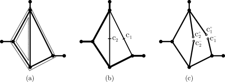
Figure 1. A graph with a choice of generators of the fundamental group (a); a choice of the spanning tree (thicker edges) and the cut points (b); the cut tree $T$ with new vertices $c_{j}^{\pm}$ (c).

We consider the $m$-th eigenvalue $\lambda_{m}(H_{\boldsymbol{\gamma}})$ as a function of $\boldsymbol{\gamma}$. We will prove that each eigenfunction $\psi_{n}$ of $H^{0}$ gives rise to a critical point of the function $\lambda_{m}(H_{\boldsymbol{\gamma}})$ (for a suitable $m$) and find the Morse index of this critical point. This problem was first considered in [9] to study the partitions of the graph $\Gamma$. The results of [9] contained an a priori condition of non-degeneracy of the critical point which rendered them unsuitable for the task of proving Theorem 1. Theorem 2 below removes this extraneous condition and generalizes the results of [9]. We discuss the connection to [9] in more detail in section 6.

Let $\lambda_{n}$ be a simple eigenvalue of $H^{0}$ and $\psi$ be the corresponding eigenfunction. Assume that the function $\psi$ is non-zero at the vertices of the graph and at the cut points $c_{j}$ (moving the cut points if necessary). Since $\psi\in\widetilde{H}^{2}(\Gamma,\mathbb{R})$, it is continuous and has continuous derivatives. Considering $\psi$ as a function on $T$, at every cut point $c^{\pm}_{j}$ we have

$$\psi(c_{j}^{+})=\psi(c_{j}^{-})\qquad\mbox{and}\qquad\psi^{\prime}(c_{j}^{+})=-\psi^{\prime}(c_{j}^{-}).$$

Theorem 2.

Let $\psi$ be the eigenfunction of $H^{0}$ that corresponds to a simple eigenvalue $\lambda_{n}(H^{0})$. We assume that $\psi$ is non-zero on vertices of the graph. We denote by $\phi$ the number of internal zeros of $\psi$ on $\Gamma$. Define

(5) $$\tilde{\gamma}_{j}:=\frac{\psi^{\prime}(c_{j}^{+})}{\psi(c_{j}^{+})}=-\frac{\psi^{\prime}(c_{j}^{-})}{\psi(c_{j}^{-})}$$

and let $\widetilde{\boldsymbol{\gamma}}=(\tilde{\gamma}_{1},\ldots,\tilde{\gamma}_{\beta})$. Consider the eigenvalues of $H_{\boldsymbol{\gamma}}$ as functions $\lambda_{n}(H_{\boldsymbol{\gamma}})$ of $\boldsymbol{\gamma}$. Then

1. $\lambda_{\phi+1}(H_{\boldsymbol{\gamma}})\Big{|}_{\boldsymbol{\gamma}=\widetilde{\boldsymbol{\gamma}}}=\lambda_{n}(H^{0})$ where $\phi$ is the number of zeros of $\psi$ on $\Gamma$,

2. $\boldsymbol{\gamma}=\widetilde{\boldsymbol{\gamma}}$ is a non-degenerate critical point of the function $\lambda_{\phi+1}(H_{\boldsymbol{\gamma}})$, and

3. the Morse index of the critical point $\boldsymbol{\gamma}=\widetilde{\boldsymbol{\gamma}}$ is equal to $n-1+\beta-\phi$.

4. Proof of Theorem 2

Before we prove Theorem 2, we collect some preliminary results in subsections 4.1 through 4.4.

4.1. Quadratic form of $H_{\boldsymbol{\gamma}}$

The quadratic form of the operator $H^{0}$ on the graph $\Gamma$ is

(6) $$h[f]=\sum_{e\in E(\Gamma)}\int_{e}\left(f^{\prime}(x)^{2}+q(x)f^{2}(x)\right)\,dx+\sum_{v\in V(\Gamma)}\chi_{v}f^{2}(v)$$

with the domain

$$D=\{f\in\widetilde{H}^{1}(\Gamma,\mathbb{R}):f\mbox{ is continuous at all vertices of $\Gamma$}\}.$$

The Dirichlet conditions, if any, are also imposed on the domain $D$. For $\boldsymbol{\gamma}\in\mathbb{R}^{\beta}$, the quadratic form of the operator $H_{\boldsymbol{\gamma}}$ acting on the tree $T$ is formally

(7) $$h_{\boldsymbol{\gamma}}[f]=h[f]+\sum_{j=1}^{\beta}\gamma_{j}\left(f^{2}(c_{j}^{+})-f^{2}(c_{j}^{-})\right)$$

with the domain

$$D_{\boldsymbol{\gamma}}=\{f\in\widetilde{H}^{1}(T,\mathbb{R}):f\mbox{ is continuous at all vertices of the tree $T$}\}.$$

Importantly, the domain $D_{\boldsymbol{\gamma}}$ is larger than $D$ since we no longer impose continuity at the cut points $c_{j}$ on the functions from $D_{\boldsymbol{\gamma}}$. More precisely, we can represent the domain $D$ as

$$D=\{f\in D_{\boldsymbol{\gamma}}:f(c_{j}^{+})=f(c_{j}^{-})\}.$$

Note that the domain $D_{\boldsymbol{\gamma}}$ is independent of the actual value of $\boldsymbol{\gamma}$.

Remark 2.

Observe that any function $f\in D_{\boldsymbol{\gamma}}$ can be written as

$$f=f_{0}+\sum_{j=1}^{\beta}s_{j}\rho_{j}$$

where $f_{0}\in D$, $s_{j}\in\mathbb{R}$ and $\rho_{j}\in D_{\boldsymbol{\gamma}}$. Moreover, we require that $\rho_{j}$ have a jump at $c_{j}$, but be continuous at all other cut points $c_{k}$, $k\neq j$ (i.e. each $\rho_{j}$ represents one jump of the function $f$). In particular, for a given $\lambda$, we will use the family of functions $\rho_{j,\lambda}$ that satisfy

$$-\rho_{j,\lambda}^{\prime\prime}(x)+(q(x)-\lambda)\rho_{j,\lambda}(x)=0$$

on every edge, the $\delta$-type conditions (1) at the vertices of $\Gamma$, and the following conditions at the cut points:

(8) $$\rho_{j,\lambda}(c_{j}^{-})=0, \rho_{j,\lambda}(c_{j}^{+})=1$$ and

(9) $$\rho_{j,\lambda}(c_{k}^{+})=\rho_{j,\lambda}(c_{k}^{-}), \rho_{j,\lambda}^{\prime}(c_{k}^{+})=-\rho_{j,\lambda}^{\prime}(c_{k}^{-})\hskip 14.45377pt\forall\hskip 3.61371ptk\neq j.$$ and

Note that condition (9) essentially glues these cut points back together.

Existence and uniqueness of the functions satisfying the above conditions is assured (see, for example [6], section 3.5.2) provided $\lambda$ stays away from the Dirichlet spectrum $\rho_{j,\lambda}(c_{j}^{+})=0$. Since we are interested in $\lambda$ close to the eignevalue $\lambda_{n}(H^{0})$ of the uncut graph, we check that $\lambda_{n}(H^{0})$ does not belong to the Dirichlet spectrum described above. The corresponding “Dirichlet graph” can be viewed as the uncut graph with an extra Dirichlet condition imposed at the vertex $c_{j}$ (in place of the Neumann condition effectively imposed there by $H^{0}$). However, by a simple extension of the interlacing theorem of [6, 17] (see Lemma 8 below for a precise formulation), one can see that the interlacing between Neumann and Dirichlet eigenvaules is strict since $\lambda_{n}(H^{0})$ is assumed to be simple and the corresponding eigenfunction $\psi$ is non-zero at the cut points.

4.2. Properties of Wronskian on graphs

It will be important to relate the values of the derivatives of the functions $\rho_{j,\lambda}$ at the cut points $c_{j}^{\pm}$. We will do this using the Wronskian. Therefore, in this subsection, we investigate the properties of the Wronskian on graphs. We will do this for the most general self-adjoint vertex conditions on the graph $\Gamma$.

Given any two functions $f_{1},f_{2}\in D$ that satisfy the differential equation $-f^{\prime\prime}(x)+(q(x)-\lambda)f(x)=0$, we know by Abel’s formula that the Wronskian of $f_{1}$ and $f_{2}$ is constant on any interval, or in particular, on any edge. Observe that the Wronskian is a one-form, that is its sign depends on direction. We will now show that the total sum of Wronskians at any vertex with self-adjoint conditions is zero (all Wronskians must be taken in the outgoing direction).

Lemma 2.

Let $\Gamma$ be a graph and let $f_{1},f_{2}\in\widetilde{H}^{2}(\Gamma,\mathbb{R})$ be two functions that satisfy the differential equation $-f^{\prime\prime}(x)+(q(x)-\lambda)f(x)=0$ and real self-adjoint vertex conditions. Then

$$\sum_{e\in E_{v}}W_{e}(f_{1},f_{2})(v)=0,$$

where $E_{v}$ denotes the set of all edges attached to the vertex $v$ and each Wronskian $W_{e}(f_{1},f_{2})$ is taken outward.

Proof.

We denote the self-adjoint operator acting as $-\frac{d^{2}}{dx^{2}}+q(x)$ by $H$. Define a smooth compactly supported function $\zeta$ on $\Gamma$ such that $\zeta\equiv 1$ in a neighborhood of the vertex $v$ and is zero at all other vertices of $\Gamma$. For the sake of convenience, we denote $\zeta f_{j}$ by $g_{j}$. Then using the self-adjointness of $H$ and integrating by parts, we obtain

$$0 =\langle Hg_{1},g_{2}\rangle-\langle g_{1},Hg_{2}\rangle$$

$$=\sum_{e\in E}\left.\left(g_{1}(x)g_{2}^{\prime}(x)-g_{1}^{\prime}(x)g_{2}(x)\right)\right|^{L_{e}}_{0}+\int_{e}\left(g_{1}^{\prime}(x)g_{2}^{\prime}(x)-g_{2}^{\prime}(x)g_{1}^{\prime}(x)\right)\,dx$$

$$=\sum_{e\in E_{v}}W_{e}(g_{1},g_{2})(v)=\sum_{e\in E_{v}}W_{e}(f_{1},f_{2})(v)$$

since $g_{j}=f_{j}$ near vertex $v$ and $g_{j}$ are zero near all other vertices. ∎

Lemma 3.

Let $a$ and $b$ be two leaves (i.e., vertices of degree one) of a graph $\Gamma$. Let $f_{1}$ and $f_{2}$ be two solutions of $-f^{\prime\prime}(x)+(q(x)-\lambda)f(x)=0$ on $\Gamma$ that satisfy the same self-adjoint vertex conditions at all vertices except $a$ and $b$. Then $W(f_{1},f_{2})(a)=-W(f_{1},f_{2})(b)$.

Proof.

In graph theory, a flow $\eta$ between two vertices $a$ and $b$ is defined as a non-negative function on the edges of a directed graph $\Gamma$ that satisfies Kirchhoff’s current conservation condition at every vertex other than $a$ or $b$: the total current flowing into a vertex must equal the total current flowing out of it (see Figure 2 for an example). Given a flow $\eta$ between $a$ and $b$, it is a standard result of graph theory that the total current flowing into $b$ is equal to the total current flowing out of $a$ [18].

We interpret the Wronskian as a flow by assigning directions to the edges of $\Gamma$ so that the Wronskian is always positive. The current conservation condition is then equivalent to Lemma 2. Therefore, the flow into $b$ equals the flow out of $a$ so $W(f_{1},f_{2})(a)=-W(f_{1},f_{2})(b)$. ∎

Figure 2. Let $\Gamma$ be the directed graph above and let $f$ be the function whose (constant) value on every edge is given by the number near each arrow. One can easily check that the function $f$ constitutes a flow on $\Gamma$.

4.3. Morse index with Lagrange multipliers

In the proof of Theorem 2, we will need to find the Morse index of the $n$-th eigenpair $(\lambda_{n},\psi)$ of $H^{0}$. The lemma below will help us to do just that.

Lemma 4.

Let $A$ be a bounded from below self-adjoint operator acting on a real Hilbert space $\mathcal{H}$. Assume that $A$ has only discrete spectrum below a certain $\Lambda$ and its eigenvalues are ordered in increasing order. Let $h[f]$ be the quadratic form corresponding to $A$. If the $n$-th eigenvalue $\lambda_{n}<\Lambda$ is simple and $\psi$ is the corresponding eigenfunction, then the Lagrange functional

(10) $$L(\lambda,f)=h[f]-\lambda(\|f\|^{2}-1)$$

has a non-degenerate critical point at $(\lambda_{n},\psi)$ whose Morse index is $n$.

Proof.

We split the Hilbert space $\mathcal{H}$ into the orthogonal sum $\mathcal{H}_{-}\oplus\mathcal{H}_{0}\oplus\mathcal{H}_{+}$. Here the space $\mathcal{H}_{-}$ is the span of the first $n-1$ eigenfunctions of $A$, the space $\mathcal{H}_{0}$ is the span of the $n$-th eigenfunction $\psi$, and $\mathcal{H}_{+}$ is their orthogonal complement. The quadratic form $h$ is reduced by the decomposition $\mathcal{H}=\mathcal{H}_{-}\oplus\mathcal{H}_{0}\oplus\mathcal{H}_{+}$, namely,

$$h\left[f_{-}+f_{0}+f_{+}\right]=h[f_{-}]+h[f_{0}]+h[f_{+}].$$

On $\mathcal{H}_{-}$, the quadratic form $h$ is bounded from above,

$$h[f_{-}]\leq\lambda_{n-1}\|f_{-}\|^{2}<\lambda_{n}\|f_{-}\|^{2}.$$

Similarly, on $\mathcal{H}_{+}$ the form $h$ is bounded from below,

$$h[f_{+}]>\lambda_{n}\|f_{+}\|^{2}.$$

Finally, on $\mathcal{H}_{0}$ we have

$$h[f_{0}]=\lambda_{n}s^{2},$$

where $f_{0}=s\psi$, $s\in\mathbb{R}$.

To show that $(\lambda_{n},\psi)$ is a critical point and calculate its index we evaluate

$$\delta L:=L(\lambda_{n}+\delta\lambda,\psi+\delta f)-L(\lambda_{n},\psi)=L(\lambda_{n}+\delta\lambda,\psi+\delta f)-\lambda_{n}.$$

Expanding $\delta f=\delta f_{-}+s\psi+\delta f_{+}$ according to our decomposition of $\mathcal{H}$, we see that

$$\delta L=h\left[\delta f_{-}\right] +\lambda_{n}(1+s)^{2}+h\left[\delta f_{+}\right]$$

$$-(\lambda_{n}+\delta\lambda)\left(\|\delta f_{-}\|^{2}+(1+s)^{2}+\|\delta f_{+}\|^{2}-1\right)-\lambda_{n}.$$

Simplifying and completing squares, we obtain

$$\delta L=\left(h\left[\delta f_{-}\right]-\lambda_{n}\|\delta f_{-}\|^{2}\right) -\frac{1}{2}(s+\delta\lambda)^{2}+\frac{1}{2}(s-\delta\lambda)^{2}$$

$$+\left(h\left[\delta f_{+}\right]-\lambda_{n}\|\delta f_{+}\|^{2}\right)+\mbox{ higher order terms},$$

where the two middle terms are representing $2s\delta\lambda$. We observe that all terms are quadratic or higher order and hence $(\lambda_{n},\psi)$ is a critical point as claimed. The first two terms represent the negative part of the Hessian. Their dimension is the dimension of $\mathcal{H}_{-}$ plus one. Thus the Morse index is $(n-1)+1=n$. ∎

We remark that in the finite-dimensional case the Hessian of $\delta L$ at the critical point is known as the “bordered Hessian” (see [19] for a brief history of the term).

4.4. Restriction to a critical manifold

We will also use the following simple result from [11].

Lemma 5.

Let $X=Y\bigoplus Y^{\prime}$ be a direct decomposition of a Banach space. Let also $f:X\to\mathbb{R}$ be a smooth functional such that $(0,0)\in X$ is its critical point of Morse index $\operatorname{ind}(f)$.

If for any $y$ in a neighborhood of zero in $Y$, the point $(y,0)$ is a critical point of $f$ over the affine subspace $\{y\}\times Y^{\prime}$, then the Hessian of $f$ at the origin, as a quadratic form in $X$, is reduced by the decomposition $X=Y\bigoplus Y^{\prime}$.

In particular,

(11) $$\operatorname{ind}(f)=\operatorname{ind}(f|_{Y})+\operatorname{ind}(f|_{Y^{\prime}}),$$

where $\operatorname{ind}(f|_{W})$ is the Morse index of $0$ as the critical point of the function $f$ restricted to the space $W$. Moreover, if $(0,0)$ is a non-degenerate critical point of $f$ on $X$, then $0$ is non-degenerate as a critical point of $f|_{Y}$.

The subspace $Y$, which is the locus of the critical points of $f$ over the affine subspaces $(y,\cdot)$, is called the critical manifold. In applications, the locus of the critical points with respect to a chosen direction is usually not a linear subspace. Then a simple change of variables is applied to reduce the situation to that of Lemma 5, while the Morse index remains unchanged.

4.5. Proof of Theorem 2

In this subsection, $\lambda$ is used as both an independent variable and a function (eigenvalue as a function of parameters). To reduce the confusion we denote $\xi=\lambda_{n}(H^{0})$. Recall that $\psi$ is the $n$-th eigenfunction of $H^{0}$ and $\phi$ denotes the number of internal zeros of $\psi$ on $\Gamma$.

Proof of Part 1 of Theorem 2.

By design, $\psi$ is an eigenfunction of $H_{\boldsymbol{\gamma}}$ when $\boldsymbol{\gamma}=\widetilde{\boldsymbol{\gamma}}$; the vertex conditions at the new vertices $c_{j}^{\pm}$ were specifically chosen to fit $\psi$. We conclude that $\xi\in\sigma\left(H_{\widetilde{\boldsymbol{\gamma}}}\right)$.

Since $\psi$ is non-zero on vertices, the corresponding eigenvalue of $H_{\widetilde{\boldsymbol{\gamma}}}$ is simple [20, 17]. Eigenfunctions on a tree are Courant-sharp [21, 20, 17]; in other words the eigenfunction number $n$ has $n-1$ internal zeros. We use this property in reverse, concluding that $\psi$ is the eigenfunction number $\phi+1$ of the tree operator $H_{\widetilde{\boldsymbol{\gamma}}}$. ∎

Proof of Part 2 of Theorem 2.

Here we prove that $\boldsymbol{\gamma}=\widetilde{\boldsymbol{\gamma}}$ is a critical point of $\lambda_{\phi+1}(H_{\boldsymbol{\gamma}})$.

Consider the Lagrange functional

(12) $$F_{3}(\lambda,f,\boldsymbol{\gamma})=h_{\boldsymbol{\gamma}}[f]-\lambda\left(\sum_{e\in E(T)}\int_{e}f^{2}(x)\,dx-1\right)$$

where $h_{\boldsymbol{\gamma}}[f]$ is the quadratic form of the operator $H_{\boldsymbol{\gamma}}$, given by equation (7). Observe that $\lambda_{\phi+1}(H_{\boldsymbol{\gamma}})=:\lambda(\boldsymbol{\gamma})$ is a restriction of $F_{3}$ onto a submanifold, namely,

(13) $$\lambda_{n}(\boldsymbol{\gamma})=F_{3}\Big{(}\lambda(\boldsymbol{\gamma}),f(\boldsymbol{\gamma}),\boldsymbol{\gamma}\Big{)},$$

where $f(\boldsymbol{\gamma})$ is the normalized $(\phi+1)$-th eigenfunction of $H_{\boldsymbol{\gamma}}$. We will now show that $(\xi,\psi,\widetilde{\boldsymbol{\gamma}})$ is a critical point of $F_{3}$; then criticality of the function $\lambda_{\phi+1}(H_{\boldsymbol{\gamma}})$ will follow immediately.

We know from Lemma 4 that the the eigenpair $(\xi,\psi)$ is a critical point of the Lagrange functional and therefore

$$\left.\frac{\partial F_{3}}{\partial\lambda}\right|_{(\lambda,f,\boldsymbol{\gamma})=(\xi,\psi,\widetilde{\boldsymbol{\gamma}})}=0\hskip 21.68121pt\mbox{and}\hskip 21.68121pt\left.\frac{\partial F_{3}}{\partial f}\right|_{(\lambda,f,\boldsymbol{\gamma})=(\xi,\psi,\widetilde{\boldsymbol{\gamma}})}=0.$$

Additionally, we calculate from equation (7) that

$$\left.\frac{\partial F_{3}}{\partial\gamma_{j}}\right|_{(\lambda,f,\boldsymbol{\gamma})=(\xi,\psi,\widetilde{\boldsymbol{\gamma}})}=\psi^{2}(c_{j}^{+})-\psi^{2}(c_{j}^{-})=0\hskip 14.45377pt\mbox{ for }j=1,\ldots,\beta,$$

since $\psi\in\widetilde{H}^{1}(\Gamma,\mathbb{R})$ is continuous at all cut points $c_{j}$. This proves that $\widetilde{\boldsymbol{\gamma}}$ is a critical point of $\lambda_{\phi+1}(H_{\boldsymbol{\gamma}})$. The non-degeneracy of the point will follow from the proof of part 3. ∎

Proof of Part 3 of Theorem 2.

We will calculate the index of the critical point $\widetilde{\boldsymbol{\gamma}}$ of $\lambda_{\phi+1}(H_{\boldsymbol{\gamma}})$ in two steps. We will first establish that the index of $(\xi,\psi,\widetilde{\boldsymbol{\gamma}})$ as a critical point of $F_{3}$ is equal to $n+\beta$. Then we will apply Lemma 5 to the restriction introduced in  (13) in order to deduce the final result. In fact the second step is simpler and we start with it to illustrate our technique.

Index of the critical point $\boldsymbol{\gamma}=\widetilde{\boldsymbol{\gamma}}$ of $\lambda(H_{\boldsymbol{\gamma}})$. Assume we have already shown that $(\xi,\psi,\widetilde{\boldsymbol{\gamma}})$ is a non-degenerate critical point of $F_{3}$ of index $n+\beta$. Define the following change of variables:

(14) $$\begin{cases}\hat{\lambda}=\lambda-\lambda(\boldsymbol{\gamma}),\\ \hat{f}=f-f(\boldsymbol{\gamma}),\\ \hat{\boldsymbol{\gamma}}=\boldsymbol{\gamma}-\widetilde{\boldsymbol{\gamma}},\end{cases}$$

where $\lambda(\boldsymbol{\gamma})$ is the $(\phi+1)$-th eigenvalue of the operator $H_{\boldsymbol{\gamma}}$ and $f(\boldsymbol{\gamma})$ is the corresponding normalized eigenfunction. The eigenvalue $\lambda(\boldsymbol{\gamma})$ is simple when $\boldsymbol{\gamma}=\widetilde{\boldsymbol{\gamma}}$ (see the proof of Part 1 above) and this property is preserved locally.

The critical point $(\xi,\psi,\widetilde{\boldsymbol{\gamma}})$ corresponds, in the new variables, to $(0,0,\boldsymbol{0})$. The change of variables is obviously non-degenerate and therefore the signature of a critical point remains unchanged.

For every fixed $\boldsymbol{\gamma}$, the function $F_{3}$ is the Lagrange functional of the operator $H_{\boldsymbol{\gamma}}$ and by Lemma 4 we conclude that $(\lambda(\boldsymbol{\gamma}),f(\boldsymbol{\gamma}))$ is its non-degenerate critical point of index $\phi+1$. In the new variables this translates to $(0,0,\hat{\boldsymbol{\gamma}})$ being a critical point with respect to the first two variables for any value of the third variable. Now we can apply Lemma 5 to conclude that $\hat{\boldsymbol{\gamma}}=\boldsymbol{0}$ is a non-degenerate critical point of $F_{3}(0,0,\hat{\boldsymbol{\gamma}})$ with index $(n+\beta)-(\phi+1)$.

Since $F_{3}(0,0,\hat{\boldsymbol{\gamma}})=\lambda_{\phi+1}(\boldsymbol{\gamma})$, we obtain the desired conclusion. It remains to verify the assumption that $(\xi,\psi,\widetilde{\boldsymbol{\gamma}})$ is a non-degenerate critical point of $F_{3}$ of index $n+\beta$.

Index of critical point of $F_{3}$. By Remark 2, any $f\in D_{\boldsymbol{\gamma}}$ can be written as

$$f=f_{0}+\sum_{j=1}^{\beta}s_{j}\rho_{j,\lambda}=:f_{0}+\boldsymbol{s}\cdot\boldsymbol{\rho_{{}_{\lambda}}},$$

where $f_{0}\in D$ and each $\rho_{j,\lambda}$ satisfies $g^{\prime\prime}(x)+(q(x)-\lambda)g(x)=0$. Therefore the Lagrange functional $F_{3}$ can be re-parametrized as follows:

$$F_{4}(\lambda,f_{0},\boldsymbol{s},\boldsymbol{\gamma}) :=F_{3}\left(\lambda,f_{0}+\boldsymbol{s}\cdot\boldsymbol{\rho_{{}_{\lambda}}},\boldsymbol{\gamma}\right)$$

$$=h_{\boldsymbol{\gamma}}[f_{0}+\boldsymbol{s}\cdot\boldsymbol{\rho_{{}_{\lambda}}}]-\lambda\left(\int_{T}\left(f_{0}+\boldsymbol{s}\cdot\boldsymbol{\rho_{{}_{\lambda}}}\right)^{2}\,dx-1\right),$$

where we understand the integral over the graph $T$ as the sum of integrals over all edges of $T$. We let

$$R_{j}(\lambda)=\rho_{j,\lambda}^{\prime}(c_{j}^{+})+\rho_{j,\lambda}^{\prime}(c_{j}^{-}),$$

and investigate $F_{4}$ as a function of $\boldsymbol{s}$ and $\boldsymbol{\gamma}$ while $\lambda$ and $f_{0}$ are held fixed. It turns out that $(\boldsymbol{s},\boldsymbol{\gamma})=(\boldsymbol{0},\boldsymbol{R})$ is a critical point. Indeed, we calculate explicitly that

$$\left.\frac{1}{2}\frac{\partial F_{4}}{\partial s_{j}}\right|_{\boldsymbol{s}=0} =\int_{T}\left(f_{0}^{\prime}\rho_{j,\lambda}^{\prime}+qf_{0}\rho_{j,\lambda}-\lambda f_{0}\rho_{j,\lambda}\right)\,dx$$

$$\hskip 85.35826pt+\gamma_{j}f_{0}(c_{j}^{+})(\rho_{j,\lambda}(c_{j}^{+})-\rho_{j,\lambda}(c_{j}^{-}))$$

$$=\int_{T}f_{0}\left(-\rho_{j,\lambda}^{\prime\prime}+(q-\lambda)\rho_{j,\lambda}\right)\,dx$$

$$\hskip 85.35826pt+f_{0}(x)\rho_{j,\lambda}^{\prime}(x)\Big{|}_{c_{j}^{-}}^{c_{j}^{+}}+\gamma_{j}f_{0}(c_{j}^{+})$$

$$=f_{0}(c_{j}^{+})\left(\gamma_{j}-\rho_{j,\lambda}^{\prime}(c_{j}^{+})-\rho_{j,\lambda}^{\prime}(c_{j}^{-})\right)$$

is equal to zero when $\gamma_{j}=R_{j}(\lambda)$. Note that we assumed $\chi_{v}=0$ at every vertex of the graph $\Gamma$. If this is not the case, the corresponding terms cancel out when the integration by parts is performed.

The partial derivatives with respect to $\gamma_{j}$ also vanish,

$$\left.\frac{\partial F_{4}}{\partial\gamma_{j}}\right|_{\boldsymbol{s}=0}=\left[f^{2}(c_{j}^{+})-f^{2}(c_{j}^{-})\right]_{\boldsymbol{s}=0}=f_{0}^{2}(c_{j}^{+})-f_{0}^{2}(c_{j}^{-})=0,$$

since the function $f_{0}\in D$ is continuous across the cut vertices $c_{j}$. Here we used the short-hand $f=f_{0}+\boldsymbol{s}\cdot\boldsymbol{\rho_{{}_{\lambda}}}$.

We can also calculate the Morse index of the critical point $(\boldsymbol{s},\boldsymbol{\gamma})=(\boldsymbol{0},\boldsymbol{R})$. The Hessian is block-diagonal with $\beta$ blocks of the form

$$\begin{bmatrix}\frac{\partial^{2}F}{\partial\gamma_{j}\partial\gamma_{j}}&\frac{\partial^{2}F}{\partial s_{j}\partial\gamma_{j}}\\ \frac{\partial^{2}F}{\partial\gamma_{j}\partial s_{j}}&\frac{\partial^{2}F}{\partial s_{j}\partial s_{j}}\\ \end{bmatrix}=\begin{bmatrix}0&2f_{0}(c_{j}^{+})\\ 2f_{0}(c_{j}^{+})&\cdot\end{bmatrix},$$

where the value of the second derivative with respect to $s_{j}$ is irrelevant. Each block has negative determinant and therefore contributes one negative and one positive eigenvalue. The total index is therefore $\beta$ and the critical point is obviously non-degenerate.

Finally, we observe that the critical manifold $(\lambda,f_{0},\boldsymbol{0},\boldsymbol{R}(\lambda))$ passes through the critical point $(\xi,\psi,\boldsymbol{0},\widetilde{\boldsymbol{\gamma}})$. To show this we need to verify that $R_{j}(\xi)=\widetilde{\boldsymbol{\gamma}}_{j}$ when $f_{0}=\psi$. Applying Lemma 3 to the Wronskian of $\psi$ and $\rho_{j}$ we obtain

$$\psi^{\prime}(c_{j}^{+})\rho_{j,\xi}(c_{j}^{+})-\rho^{\prime}_{j,\xi}(c_{j}^{+})\psi(c_{j}^{+})=-\psi^{\prime}(c_{j}^{-})\rho_{j,\lambda}(c_{j}^{-})+\rho^{\prime}_{j,\xi}(c_{j}^{-})\psi(c_{j}^{-}).$$

Substituting the boundary values of $\rho_{j}$ (see Remark 2), we arrive at

$$\tilde{\gamma_{j}}:=\frac{\psi^{\prime}(c_{j}^{+})}{\psi(c_{j}^{+})}=\rho^{\prime}_{j,\xi}(c_{j}^{+})+\rho^{\prime}_{j,\xi}(c_{j}^{-})=:R_{j}.$$

By using the non-degenerate change of variables

(15) $$\begin{cases}\hat{\lambda}=\lambda-\xi,\\ \hat{f}=f_{0}-\psi,\\ \hat{\boldsymbol{s}}=\boldsymbol{s}-\boldsymbol{0},\\ \hat{\boldsymbol{\gamma}}=\boldsymbol{\gamma}-\boldsymbol{R}(\lambda),\end{cases}$$

we can again apply Lemma 5 with $Y=\big{\{}(\hat{\lambda},\hat{f},\boldsymbol{0},\boldsymbol{0})\big{\}}$. On the subspace $Y$, the function $F_{3}$ is equal to $h[f_{0}]-\lambda\left(\|f_{0}\|^{2}-1\right)$, which is precisely the Lagrange functional for the operator $H^{0}$ with the correct domain. By Lemma 4 it has index $n$ at the point $(\lambda,f_{0})=(\xi,\psi)$. Adding the two indices together we obtain index $n+\beta$ for the critical point $(\xi,\psi,\boldsymbol{0},\widetilde{\boldsymbol{\gamma}})$ of $F_{4}$, which corresponds to the critical point $(\xi,\psi,\widetilde{\boldsymbol{\gamma}})$ of $F_{3}$. This concludes our proof. ∎

5. Critical Points of $\lambda_{n}(H^{\boldsymbol{\alpha}})$

In this section we show that $\boldsymbol{\alpha}=(0,\ldots,0)$ is a critical point of $\lambda(H^{\boldsymbol{\alpha}})$ and compute its Morse index, thus concluding the proof of Theorem 1.

5.1. Points of symmetry

Theorem 3.

Let $\sigma(\boldsymbol{\alpha})$ denote the spectrum of $H^{\boldsymbol{\alpha}}$ where $\boldsymbol{\alpha}=(\alpha_{1},\ldots,\alpha_{\beta})\in\mathbb{R}^{\beta}$. Then all points in the set

(16) $$\Sigma=\left\{\pi(b_{1},\ldots,b_{\beta}):b_{j}\in\{0,1\}\right\}$$

are points of symmetry of $\sigma(\boldsymbol{\alpha})$, i.e. for all $\boldsymbol{\alpha}\in\mathbb{R}^{\beta}$ and for all $\boldsymbol{\varsigma}\in\Sigma$,

(17) $$\sigma(\boldsymbol{\varsigma}-\boldsymbol{\alpha})=\sigma(\boldsymbol{\varsigma}+\boldsymbol{\alpha}),$$

together with multiplicity.

Consequently, if $\lambda_{n}(\boldsymbol{\alpha})$ is the $n$-th eigenvalue of $H^{\boldsymbol{\alpha}}$ that is simple at $\boldsymbol{\alpha}=\boldsymbol{\varsigma}\in\Sigma$, then $\boldsymbol{\varsigma}$ is a critical point of the function $\lambda_{n}(\boldsymbol{\alpha})$.

Proof.

We will show that if $f(x)$ is an eigenfunction of $H^{\boldsymbol{\varsigma}-\boldsymbol{\alpha}}$, then $\overline{f(x)}$ is an eigenfunction of $H^{\boldsymbol{\varsigma}+\boldsymbol{\alpha}}$. Since the operator $H^{\boldsymbol{\alpha}}$ is self-adjoint, we know that the eigenvalues are real. Taking the complex conjugate of the eigenvalue equation for $f$ we see that $\overline{f(x)}$ satisfies the same equation,

$$-\frac{d^{2}\overline{f(x)}}{dx^{2}}+q(x)\overline{f(x)}=\lambda\overline{f(x)}.$$

Similarly, all vertex conditions at the vertices of the tree $T$ inherited from $\Gamma$ have real coefficients and therefore $\overline{f(x)}$ satisfies them too. The only change occurs at the vertices $c^{\pm}_{j}$.

Note that for every $\boldsymbol{\sigma}\in\Sigma$, $\sigma_{j}$ is equal to either $0$ or $\pi$ so $e^{2i\sigma_{j}}=1$ for all $j=1,\ldots,\beta$. Therefore,

$$\overline{e^{i(\sigma_{j}-\alpha_{j})}}=e^{i(-\sigma_{j}+\alpha_{j})}=e^{i(\sigma_{j}+\alpha_{j})}e^{-2i\sigma_{j}}=e^{i(\sigma_{j}+\alpha_{j})}.$$

Conjugating the vertex conditions of $H^{\boldsymbol{\varsigma}-\boldsymbol{\alpha}}$ at $c^{\pm}_{j}$ we obtain

$$\overline{f(c_{j}^{-})}=\overline{e^{i(\sigma_{j}-\alpha_{j})}f(c_{j}^{+})}=e^{i(\sigma_{j}+\alpha_{j})}\overline{f(c_{j}^{+})},$$

and same for the derivative. Thus $\overline{f(x)}$ satisfies the vertex conditions of the operator $H^{\boldsymbol{\varsigma}+\boldsymbol{\alpha}}$ and vice versa. The spectra of these two operators are therefore identical. ∎

5.2. A non-self-adjoint continuation

We now consider the same operator $-\frac{d^{2}}{dx^{2}}+q(x)$ on the tree $T$ with different vertex conditions at $c_{j}^{\pm}$:

(18) $$\begin{split}f(c_{j}^{+})&=e^{\alpha_{j}}f(c_{j}^{-}),\\ f^{\prime}(c_{j}^{+})&=-e^{\alpha_{j}}f^{\prime}(c_{j}^{-}),\end{split}$$

i.e. the function has a jump in magnitude across the cut. It is easy to see that these conditions are obtained from (2) by changing $\boldsymbol{\alpha}$ to $-i\boldsymbol{\alpha}$. We will denote the operator with vertex conditions $\eqref{eq:real_jump_cond}$ at the vertices in $T\backslash\Gamma$ by $H^{i\boldsymbol{\alpha}}$.

Remark 3.

The operator of $H^{i\boldsymbol{\alpha}}$ is not self-adjoint for $\boldsymbol{\alpha}\in\mathbb{R}^{\beta}$. A simple example is the interval $[0,\pi]$ with $q(x)=0$ and conditions

$$f(0)=e^{\alpha}f(\pi)\qquad\mbox{and}\qquad f^{\prime}(0)=e^{\alpha}f^{\prime}(\pi),$$

which has complex eigenvalues when $\alpha\neq 0$. Indeed, the eigenvalues are easily calculated to be

$$\lambda_{n}=\left(2n\pm\frac{\alpha}{\pi}i\right)^{2}.$$

Lemma 6.

If $\lambda_{n}(H^{0})$ is simple, then locally around $\boldsymbol{\alpha}=(0,\ldots,0)$ the eigenvalue $\lambda_{n}(H^{i\boldsymbol{\alpha}})$ is real. The corresponding eigenfunction is real too.

Proof.

By standard perturbation theory [22] (see also [17] for results specifically on graphs) we know that $\lambda_{n}(H^{i\boldsymbol{\alpha}})$ is an analytic function of $\boldsymbol{\alpha}$ and since $\lambda_{n}(H^{0})$ is simple, $\lambda_{n}(H^{i\boldsymbol{\alpha}})$ remains simple in a neighborhood of $\boldsymbol{\alpha}=(0,\ldots,0)$. Since the operator $H^{i\boldsymbol{\alpha}}$ has real coefficients, its complex eigenvalues must come in conjugate pairs. For this to happen, the real eigenvalue must first become double. Since $\lambda_{n}(H^{i\boldsymbol{\alpha}})$ is simple near $(0,\ldots,0)$, the eigenvalue is real there. ∎

We note that since we impose no restrictions on the eigenvalues below $\lambda_{n}(H^{0})$, some of them might turn complex as soon as $\boldsymbol{\alpha}\neq 0$. In this case, the “$n$-th” eigenvalue $\lambda_{n}(H^{i\boldsymbol{\alpha}})$ refers to the unique continuation of $\lambda_{n}(H^{0})$. Locally, of course, it is the same as having the eigenvalues ordered by their real part.

5.3. Connection between $H_{\boldsymbol{\gamma}}$ and $H^{i\boldsymbol{\alpha}}$

Locally around $\boldsymbol{\gamma}=\widetilde{\boldsymbol{\gamma}}$ we introduce a mapping $R:\boldsymbol{\gamma}\mapsto\boldsymbol{\alpha}$ so that $\lambda_{\phi+1}\left(H_{\boldsymbol{\gamma}}\right)=\lambda_{n}\left(H^{i\boldsymbol{\alpha}}\right)$ when $R(\boldsymbol{\gamma})=\boldsymbol{\alpha}$.

For a given $\boldsymbol{\gamma}$, we find the $(\phi+1)$-th eigenfunction of $H_{\boldsymbol{\gamma}}$, denoting it by $g$. We then let

(19) $$e^{\alpha_{j}}=\frac{g(c_{j}^{+})}{g(c_{j}^{-})}$$

and, since $g$ satisfies equation (4), it is now easy to check that $g$ is indeed an eigenfunction of $H^{i\boldsymbol{\alpha}}$.

Lemma 7.

The function $R$ is a non-degenerate diffeomorphism. Therefore, the point $\boldsymbol{\alpha}=(0,\ldots,0)$ is a critical point of the function $\lambda_{n}\left(H^{i\boldsymbol{\alpha}}\right)$ of index $n-1+\beta-\phi$.

Proof.

The function $R$ is an analytic function in a neighborhood of $\widetilde{\boldsymbol{\gamma}}$ since the eigenfunctions are analytic functions of the parameters and therefore $R$ is a composition of analytic functions. We can define $R^{-1}$ by reversing the process, i.e. for a given $\boldsymbol{\alpha}$ find the (real) $n$-th eigenfunction $\varphi$ of $H^{i\boldsymbol{\alpha}}$ and let $\gamma_{j}=\varphi^{\prime}(c^{+}_{j})/\varphi(c^{+}_{j})$. By the same arguments, $R^{-1}$ is also an analytic function in a neighborhood of $(0,\ldots,0)$. Therefore $R$ is a non-degenerate diffeomorphism.

A diffeomorphism preserves the index and therefore the index of $(0,\ldots,0)$ of the function $\lambda_{n}\left(H^{i\boldsymbol{\alpha}}\right)$ is the same as the index of $\widetilde{\boldsymbol{\gamma}}$ of the function $\lambda_{\phi+1}\left(H_{\boldsymbol{\gamma}}\right)$, which was computed in Theorem 2. ∎

5.4. From $H^{i\boldsymbol{\alpha}}$ to $H^{\boldsymbol{\alpha}}$

Proof of Theorem 1.

The function $\lambda_{n}(H^{\boldsymbol{\alpha}})-\xi$ is analytic and, locally around $(0,\ldots,0)$, quadratic in $\{\alpha_{j}\}$ because $(0,\ldots,0)$ is a critical point so the linear term (the first derivative) is zero. Substituting $\boldsymbol{\alpha}\to-i\boldsymbol{\alpha}$ into the quadratic term results in an overall minus, that is

$$\lambda_{n}(H^{i\boldsymbol{\alpha}})-\xi=-\left(\lambda_{n}(H^{\boldsymbol{\alpha}})-\xi\right)+\mbox{higher order terms}.$$

Therefore the index of $(0,\ldots,0)$ as a critical point of $\lambda_{n}(H^{\boldsymbol{\alpha}})$ is the dimension of the space of variables minus the index of $\lambda_{n}(H^{i\boldsymbol{\alpha}})$. Thus it is equal to

$$\beta-(n-1+\beta-\phi)=\phi-(n-1).$$

∎

6. Connection to partitions on graphs

The set of points on which a real eigenfunction vanishes (called the nodal set) generically has co-dimension 1. Thus, when one considers a problem which is not 1-dimensional (or quasi-1-dimensional, like a graph), counting the number of zeros does not make sense. Then one usually counts the number of “nodal domains”: the connected components obtained after removing the nodal set from the domain. We refer to the number of nodal domains as the nodal domain count. It should be noted that the nodal domain count is a non-local property [7]. Let $\nu_{n}$ denote the number of nodal domains of the $n$-th eigenfunction. Then a classical result of Courant [23, 24], in the case of the Dirichlet Laplacian, bounds $\nu_{n}$ from above by $n$, independently of dimension.

An interesting new point of view on the nodal domains arose recently, see [25] and references therein. Namely, a domain is partitioned into subdomains and the following question is asked: when does a given partition coincide with the nodal partition corresponding to an eigenfunction of the Dirichlet Laplacian on the original domain? It turns out that there is a natural “energy” functional defined on partitions whose minima correspond to the eigenfunctions satisfying $\nu_{n}=n$. Restricting the set of allowed partitions, it was further found [9, 10, 11] that all critical points of this functional correspond to eigenfunctions and the “nodal deficiency” $n-\nu_{n}$ is equal to the Morse index of the critical point (which is zero for a minimum).

The latter result was first established on graphs in [9] and here we outline how its strengthened version follows from our Theorem 2. We define a proper $m$-partition $P$ of a graph $\Gamma$ as a set of $m$ points lying on the edges of the graph (and not on the vertices). Enforcing Dirichlet conditions at these vertices effectively separates the graph $\Gamma$ into partition subgraphs which we will denote $\Gamma_{j}$. The functional mentioned above is defined as

(20) $$\Lambda(P):=\max_{j}\lambda_{1}(\Gamma_{j}),$$

where $\lambda_{1}(\Gamma_{j})$ is the first eigenvalue of the partition subgraph $\Gamma_{j}$. The conditions on the vertices of $\Gamma_{j}$ are either inherited from $\Gamma$ or taken to be Dirichlet on the newly formed vertices.

The partition $P$ should be understood as a candidate for the nodal set of an eigenfunction of $\Gamma$. It is easy to see that the partition points break every cycle of $\Gamma$ if and only if the number $\nu(P)$ of the partition subgraphs is related to $m$ by

(21) $$\nu(P)=m-\beta+1.$$

We start by considering the partitions and eigenfunctions that satisfy the above property. In section 6.1 we will treat the case of partitions where some of the cycles survive.

Further, we call an $m$-partition an equipartition if all subgraphs $\Gamma_{j}$ share the same eigenvalue:

$$\lambda_{1}(\Gamma_{j_{1}})=\lambda_{1}(\Gamma_{j_{2}}),\qquad\mbox{for all }j_{1},j_{2}.$$

It is easy to see that the partition defined by the nodal set of an eigenfunction is an equipartition. In [9] it was shown that the set of $m$-equipartitions on $\Gamma$ can be parametrized using $\beta$ parameters $\{\gamma_{j}\}$ and the operator $H_{\boldsymbol{\gamma}}$ defined in section 3: we take the $(m+1)$-th eigenfunction of $H_{\boldsymbol{\gamma}}$ and its zeros (transplanted to the original graph $\Gamma$) define an equipartition. With such parametrization, the energy $\Lambda(P)$ of the partition is simply the $(m+1)$-th eigenvalue $\lambda_{m+1}(H_{\boldsymbol{\gamma}})$. Now Theorem 2 immediately implies the following.

Corollary 1.

Suppose the $n$-th eigenvalue of $\Gamma$ is simple and its eigenfunction $\psi$ is non-zero on vertices. Denote by $\phi$ the number of zeros of $\psi$ and by $\nu$ the number of its nodal domains. If the zeros of the eigenfunction break every cycle of $\Gamma$, then the $\phi$-partition defined by the zeros of $\psi$ is a non-degenerate critical point of the functional $\Lambda$ on the set of equipartitions. The Morse index of the critical point is equal to $n-\nu$.

Some remarks are in order. The “converse” fact that critical points of $\Lambda$ correspond to eigenfunctions is easy to establish. The main difficulty lies in calculating the Morse index. In the main theorem of [9], the non-degeneracy of the critical point had to be assumed a priori. In section 4, we established that this actually follows from the other assumptions. Eigenfunctions whose zeros do not break all cycles of $\Gamma$ correspond to low values of $\lambda$, and it can easily be shown that there are only finitely many such eigenfunctions. We will handle these eigenfunctions by introducing cut points only on those cycles which are broken by the zeros of $\psi$ and correspondingly adjusting the operator $H_{\boldsymbol{\gamma}}$. Finally, the mapping $R$ defined in section 5.3 essentially shows that the equipartitions can be parameterized using eigenfunctions of the “magnetic” Schrödinger operator with purely imaginary magnetic field.

6.1. Partitions with few zeros

For eigenfunctions corresponding to low eigenvalues, the nodal set might not break all the cycles of the graph, see Fig. 3(a). In this case, the parameterization of the nearby equipartitions is done via a modification of the operator $H_{\gamma}$. In this section we describe this parameterization and point out the changes in the proofs of the analogue of Theorem 2 that the new parameterization necessitates. An outline of the procedure has already appeared in [9, 10]; however some essential details have been omitted there.

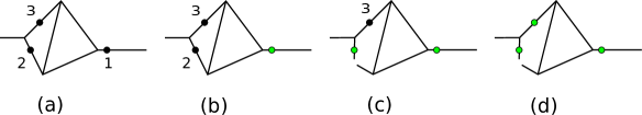
Figure 3. A partition with surviving cycles. (a) Zeros, marked 1, 2, and 3, do not lie on all the cycles of the graph. To find cut points we consider the zeros in sequence. (b) Cutting the graph at zero 1 would disconnect it. (c) Cutting the graph at zero 2 would not disconnect it; therefore, a cut point is placed nearby. (d) Now, cutting the graph at zero 3 would disconnect the graph, so we do not introduce any more cut points.

As mentioned previously, the eigenfunctions we are interested in here do not have a zero on every cycle. Hence, unlike the previous case for large eigenvalues where the corresponding eigenfunctions have at least one zero on every cycle, we must carefully pick our cut points to avoid cutting cycles that do not contain any zeros of the eigenfunction. To do this we look at the zeros of our eigenfunction $\psi$ one at a time. If cutting the edge that contains the zero will disconnect the graph, we do nothing and remove this zero from consideration (see Fig. 3(b)). If cutting the edge at the zero will not disconnect the graph, then we cut that edge at a nearby point $c_{j}$ at which $\psi$ is non-zero, calling the new vertices $c_{j}^{+}$ and $c_{j}^{-}$ as before (see Fig. 3(c)). Notice that the manner in which we order and analyze the zeros does not matter; while the cut positions and resulting graph may vary, we will make the same number of cuts.

Let us consider the number of cuts $\eta$ more explicitly. Denote by $\mathcal{N}$ the zero set of $\psi$ and remove $\mathcal{N}$ from $\Gamma$ to get the (disconnected) graph $\Gamma\backslash\mathcal{N}$. Let $\nu$ be the number of connected components {$\Gamma_{j}$} after the cutting (the components $\Gamma_{j}$ are the nodal domains of $\Gamma$ with respect to $\psi$). Denote

$$\beta_{\Gamma\backslash\mathcal{N}}=\sum_{i=1}^{\nu}\beta_{\Gamma_{j}}$$

where $\beta_{\kappa}$ is the Betti number of the graph $\kappa$. It is easy to see that

(22) $$\eta=\beta_{\Gamma}-\beta_{\Gamma\backslash\mathcal{N}}$$

and furthermore

(23) $$\eta=1+\phi-\nu.$$

For further details, see Lemma 5.2.1 of [6]. Now we continue with an alternative statement of Theorem 2.

Theorem 4.

Let $\psi$ be the eigenfunction of $H^{0}$ that corresponds to a simple eigenvalue $\lambda_{n}(H^{0})$. We assume that $\psi$ is non-zero on internal vertices of the graph. We denote by $\phi$ the number of internal zeros and $\nu$ the number of nodal domains of $\psi$ on $\Gamma$. Let $c_{j}^{\pm}$, $j=1,\ldots,\eta$, be the cut points created by following the procedure above, where $\eta=1+\phi-\nu$.

Let $H_{\boldsymbol{\gamma}}$, $\boldsymbol{\gamma}=(\gamma_{1},\ldots,\gamma_{\eta})$, be the operator obtained from $H^{0}$ by imposing the additional conditions

(24) $$\begin{split}f^{\prime}(c_{j}^{+})&=\gamma_{j}f(c_{j}^{+}),\\ f^{\prime}(c_{j}^{-})&=-\gamma_{j}f(c_{j}^{-}),\end{split}$$

at the cut points.

Define

$$\tilde{\gamma}_{j}:=\frac{\psi^{\prime}(c_{j}^{+})}{\psi(c_{j}^{+})}=-\frac{\psi^{\prime}(c_{j}^{-})}{\psi(c_{j}^{-})}$$

and let $\widetilde{\boldsymbol{\gamma}}=(\tilde{\gamma}_{1},\ldots,\tilde{\gamma}_{\eta})$. Consider the eigenvalues of $H_{\boldsymbol{\gamma}}$ as functions $\lambda_{n}(H_{\boldsymbol{\gamma}})$ of $\boldsymbol{\gamma}$. Then

1. $\lambda_{\phi+1}(H_{\boldsymbol{\gamma}})\Big{|}_{\boldsymbol{\gamma}=\widetilde{\boldsymbol{\gamma}}}=\lambda_{n}(H^{0})$ where $\phi$ is the number of zeros of $\psi$ on $\Gamma$,

2. $\boldsymbol{\gamma}=\widetilde{\boldsymbol{\gamma}}$ is a non-degenerate critical point of the function $\lambda_{\phi+1}(H_{\boldsymbol{\gamma}})$, and

3. the Morse index of the critical point $\boldsymbol{\gamma}=\widetilde{\boldsymbol{\gamma}}$ is equal to $n-\nu$.

We will map out the proof of the theorem in section 6.2 below, after explaining its significance to the question of equipartitions.

Theorem 5.

Suppose the $n$-th eigenvalue of $\Gamma$ is simple and its eigenfunction $\psi$ is non-zero on vertices. Denote by $\phi$ the number of internal zeros of $\psi$ and by $\nu$ the number of its nodal domains. Then the $\phi$-equipartitions in the vicinity of the nodal partition of $\psi$ are parametrized by the variables $\boldsymbol{\gamma}=(\gamma_{1},\ldots,\gamma_{\eta})$.

The nodal partition of $\psi$ corresponds to the point $\widetilde{\boldsymbol{\gamma}}=(\tilde{\gamma}_{1},\ldots,\tilde{\gamma}_{\eta})$ and is a non-degenerate critical point of the functional $\Lambda$ (equation (20)) on the set of equipartitions. The Morse index of the critical point is equal to $n-\nu$.

The mapping from $(\gamma_{1},\ldots,\gamma_{\eta})$ to the equipartitions is constructed as follows (see [9] for more details): the partition in question is generated by the zeros of the $(\phi+1)$-th eigenfunction of the operator $H_{\boldsymbol{\gamma}}$ placed upon the original graph $\Gamma$. Indeed, the groundstates of the nodal domains can be obtained by cutting the eigenfunction at zeros and gluing the cut points together (conditions (24) ensure the gluing is possible). To verify that all equipartitions are obtainable in this way we simply reverse the process and construct an eigenfunction of $H_{\boldsymbol{\gamma}}$ from the groundstates of the nodal domains. The gluing is now done at zeros, and it can be done recursively (since all cycles with zeros on them have been cut).

Once the parameterization of the equipartitions is accomplished, the Morse index result follows immediately from Theorem 4.

6.2. Proof of Theorem 4

The proof of Theorem 4 is identical to the proof of Theorem 2 once we collect some preliminary results. The following lemma can be found in [6] (Theorem 3.1.8 with a slight modification).

Lemma 8.

Let $\Gamma_{\alpha^{\prime}}$ be the graph obtained from the graph $\Gamma_{\alpha}$ by changing the coefficient of the $\delta$-type condition at a vertex $v$ from $\alpha$ to $\alpha^{\prime}$ (conditions at all other vertices are fixed). If $-\infty<\alpha<\alpha^{\prime}\leq\infty$ (where $\alpha^{\prime}=\infty$ corresponds to the Dirichlet condition at vertex $v$), then

(25) $$\lambda_{n}(\Gamma_{\alpha})\leq\lambda_{n}(\Gamma_{\alpha^{\prime}})\leq\lambda_{n+1}(\Gamma_{\alpha}).$$

If the eigenvalue $\lambda_{n}(\Gamma_{\alpha^{\prime}})$ is simple and its eigenfunction $f$ is such that either $f(v)$ or $\sum f^{\prime}(v)$ is non-zero, then the above inequalities can be made strict. If, in addition, $\alpha^{\prime}\neq\infty$, the inequalities become

$$\lambda_{n}(\Gamma_{\alpha})<\lambda_{n}(\Gamma_{\alpha^{\prime}})<\lambda_{n}(\Gamma_{\infty})\leq\lambda_{n+1}(\Gamma_{\alpha}).$$

The following theorem is a generalization of Corollary 3.1.9 of [6].

Theorem 6.

Let $\Gamma$ be a graph with $\delta$-type conditions at every internal vertex and extended $\delta$-type conditions on all leaves. Suppose an eigenvalue $\lambda$ of $\Gamma$ has an eigenfunction $f$ which is non-zero on internal vertices of $\Gamma$. Further, assume that no zeros of $f$ lie on the cycles of $\Gamma$. Then the eigenvalue $\lambda$ is simple and $f$ is eigenfunction number $\phi+1$, where $\phi$ is the number of internal zeros of $f$.

Remark 4.

The condition that no zeros lie on the cycles of the graph $\Gamma$ is equivalent to $\eta=0$ (see equation (22)) or to the number of nodal domains of $f$ being equal to $\phi+1$.

Proof.

We use induction on the number of internal zeros of $f$ to show that the eigenvalue is simple. If $f$ has no internal zeros, then we know $f$ corresponds to the groundstate eigenvalue, which is simple.

Now suppose $f$ has $\phi>0$ internal zeros. By way of contradiction, assume that $\lambda$ is not simple. Choose an arbitrary zero $\zeta$ of $f$ and another eigenfunction $g$. Cut $\Gamma$ at $\zeta$; making this cut will disconnect the graph into two subgraphs since $\zeta$ cannot lie on a cycle of $\Gamma$. On at least one of these subgraphs, $g$ is non-zero and not a multiple of $f$ (otherwise, it cannot be a different eigenfunction). We will now analyze the eigenfunctions on this subgraph $\Gamma^{\prime}$.

On the graph $\Gamma^{\prime}$, $f$ and $g$ satisfy the same $\delta$-type conditions at all vertices except possibly the new leaf $\zeta$. We denote by $\Gamma^{\prime}_{\tau}$ as the graph $\Gamma^{\prime}$ with the conditions $\Phi^{\prime}(\zeta)=\tau\Phi(\zeta)$. We know that $(\lambda,f)$ is an eigenpair on $\Gamma^{\prime}_{\infty}$ and similarly, there exists $\alpha$ such that $(\lambda,g)$ is an eigenpair on $\Gamma^{\prime}_{\alpha}$. However, since $\Gamma^{\prime}_{\infty}$ contains fewer internal zeros of $f$ than $\Gamma$ does, by the inductive hypothesis $\lambda$ is simple on $\Gamma^{\prime}_{\infty}$ so $\alpha\neq\infty$.

Observe that $f^{\prime}(\zeta)$ is non-zero; if it was, the function $f$ would be identically zero on the whole edge containing $\zeta$ and, therefore, at the end-vertices of the edge. Thus, the inequalities in (25) with $\alpha^{\prime}=\infty$ become strict and $\Gamma^{\prime}_{\alpha}$ and $\Gamma^{\prime}_{\infty}$ cannot have the same eigenvalue $\lambda$.

Now we show that $f$ is eigenfunction number $n=\phi+1$. By Remark 4 there are $\nu=\phi+1$ nodal domains. Since $\lambda$ is simple, we know from Theorem 5.2.8 of [6] that

$$n-\beta\leq\nu\leq n\qquad\mbox{and}\qquad n\leq\phi+1\leq n+\beta$$

where $\beta$ is the Betti number of $\Gamma$. However, since $\nu=\phi+1$, both inequalities hold only if $\nu=n=\phi+1$ so $f$ is indeed the eigenfunction number $\phi+1$. ∎

Below we only include the parts of the proof that differ from Theorem 2.

Proof of Theorem 4.

In the proof of Theorem 2 (section 4.5), the fact that $H_{\boldsymbol{\gamma}}$ is an operator on a tree was used to show that its eigenvalue is simple and to find the sequence number of $\lambda$ in the spectrum. Theorem 6 allows us to do the same in the graph with fewer cuts.

Indeed, on the cut graph $\Gamma_{\widetilde{\boldsymbol{\gamma}}}$, $\psi$ is non-zero on all cycles and internal vertices and therefore by Theorem 6, the eigenvalue is simple and has number $\phi+1$ in the spectrum of $H_{\boldsymbol{\widetilde{\gamma}}}$. Since the eigenvalue is simple, we can still apply Lemma 4. The rest of the proof goes through, with the amendment that the index of the critical point of $F_{3}$ is $n+\eta$, since we now have $\eta$ cuts instead of $\beta$ cuts. Using equation (23), we finally get that the Morse index of the critical point is

$$(n+\eta)-(\phi-1)=n+(1+\phi-\nu)-\phi-1=n-\nu.$$

∎

References

- [1] Kuchment, P. (2002) Graph models for waves in thin structures. Waves Random Media, 12, R1–R24.
- [2] Gnutzmann, S. and Smilansky, U. (2006) Quantum graphs: Applications to quantum chaos and universal spectral statistics. Adv. Phys., 55, 527–625.
- [3] Kuchment, P. (2008) Quantum graphs: an introduction and a brief survey. Analysis on graphs and its applications, vol. 77 of Proc. Sympos. Pure Math., pp. 291–312, Amer. Math. Soc.
- [4] Berkolaiko, G., Carlson, R., Fulling, S., and Kuchment, P. (eds.) (2006) Quantum graphs and their applications, vol. 415 of Contemp. Math., Amer. Math. Soc.
- [5] Exner, P., Keating, J. P., Kuchment, P., Sunada, T., and Teplyaev, A. (eds.) (2008) Analysis on graphs and its applications, vol. 77 of Proc. Sympos. Pure Math., Amer. Math. Soc.
- [6] Berkolaiko, G. and Kuchment, P. (2013) Introduction to Quantum Graphs, vol. 186 of Mathematical Surveys and Monographs. Amer. Math. Soc.
- [7] Band, R., Oren, I., and Smilansky, U. (2008) Nodal domains on graphs—how to count them and why? Analysis on graphs and its applications, vol. 77 of Proc. Sympos. Pure Math., pp. 5–27, Amer. Math. Soc.
- [8] Band, R., Berkolaiko, G., and Smilansky, U. (2012) Dynamics of nodal points and the nodal count on a family of quantum graphs. Ann. Henri Poincaré, 13, 145–184.
- [9] Band, R., Berkolaiko, G., Raz, H., and Smilansky, U. (2012) The number of nodal domains on quantum graphs as a stability index of graph partitions. Comm. Math. Phys., 311, 815–838.
- [10] Berkolaiko, G., Raz, H., and Smilansky, U. (2012) Stability of nodal structures in graph eigenfunctions and its relation to the nodal domain count. J. Phys. A, 45, 165203.
- [11] Berkolaiko, G., Kuchment, P., and Smilansky, U. (2012) Critical partitions and nodal deficiency of billiard eigenfunctions. Geom. Funct. Anal., 22, 1517–1540, also arXiv:1107.3489 [math-ph].
- [12] Berkolaiko, G. (2013) Nodal count of graph eigenfunctions via magnetic perturbation. Anal. PDE, 6, 1213–1233, also arXiv:1110.5373 [math-ph].
- [13] Colin de Verdière, Y. (2012) Magnetic interpretation of the nodal defect on graphs. Anal. PDE, 6, 1235–1242, also arXiv:1201.1110 [math-ph].
- [14] Band, R. (2014) The nodal count {0, 1, 2, 3, …} implies the graph is a tree. Phil. Trans. Roy. Soc. A, 372, 20120504, also arXiv:1212.6710 [math-ph].
- [15] Kostrykin, V. and Schrader, R. (2003) Quantum wires with magnetic fluxes. Comm. Math. Phys., 237, 161–179.
- [16] Rueckriemen, R. (2011) Recovering quantum graphs from their Bloch spectrum, to appear in Ann. Inst. Fourier, preprint arXiv:1101.6002.
- [17] Berkolaiko, G. and Kuchment, P. (2012) Dependence of the spectrum of a quantum graph on vertex conditions and edge lengths. Spectral Geometry, vol. 84 of Proceedings of Symposia in Pure Mathematics, Amer. Math. Soc., preprint arXiv:1008.0369.
- [18] Bollobás, B. (1998) Modern graph theory, vol. 184 of Graduate Texts in Mathematics. Springer-Verlag.
- [19] Spring, D. (1985) On the second derivative test for constrained local extrema. Amer. Math. Monthly, 92, 631–643.
- [20] Schapotschnikow, P. (2006) Eigenvalue and nodal properties on quantum graph trees. Waves Random Complex Media, 16, 167–178.
- [21] Pokornyĭ, Y. V., Pryadiev, V. L., and Al′-Obeĭd, A. (1996) On the oscillation of the spectrum of a boundary value problem on a graph. Mat. Zametki, 60, 468–470.
- [22] Kato, T. (1976) Perturbation theory for linear operators. Springer-Verlag, second edn., Grundlehren der Mathematischen Wissenschaften, Band 132.
- [23] Courant, R. (1923) Ein allgemeiner Satz zur Theorie der Eigenfuktionen selbstadjungierter Differentialausdrücke. Nachr. Ges. Wiss. Göttingen Math Phys, pp. 81–84.
- [24] Courant, R. and Hilbert, D. (1953) Methods of mathematical physics. Vol. I. Interscience Publishers, Inc., New York, N.Y.
- [25] Helffer, B., Hoffmann-Ostenhof, T., and Terracini, S. (2009) Nodal domains and spectral minimal partitions. Ann. Inst. H. Poincaré Anal. Non Linéaire, 26, 101–138.