Discrete Toeplitz/Hankel determinants and the width of non-intersecting processes

Abstract

We show that the ratio of a discrete Toeplitz/Hankel determinant and its continuous counterpart equals a Freholm determinant involving continuous orthogonal polynomials. This identity is used to evaluate a triple asymptotic of some discrete Toeplitz/Hankel determinants which arise in studying non-intersecting processes. We show that the asymptotic fluctuations of the width of such processes are given by the GUE Tracy-Widom distribution. This result leads us to an identity between the GUE Tracy-Widom distribution and the maximum of the sum of two independent Airy processes minus a parabola. We provide an independent proof of this identity.

1 Introduction

This paper consists of two parts. First, we develop a general method for an asymptotic analysis of the Toeplitz or Hankel determinants of discrete measure using orthogonal polynomials with respect to a continuous measure. In the second part, which is longer, we evaluate the limiting distribution of the “width” of non-intersecting processes as an application. This leads to the discovery of an interesting identity between the GUE Tracy-Widom distribution and the maximum of the sum of two independent Airy processes minus a parabola: see Theroem 1.3.

1.1 Discrete Toeplitz determinants

For a finite subset $\mathcal{D}$ of the unit circle $\Sigma$ in the complex plane and a function $f:\mathcal{D}\to\mathbb{R}$, the Toeplitz determinant of the discrete measure $\frac{1}{|\mathcal{D}|}\sum_{z\in\mathcal{D}}f(z)\delta_{z}$ is defined as

$$\mathbf{T}_{n}(f,\mathcal{D})=\det\bigg{[}\frac{1}{|\mathcal{D}|}\sum_{z\in\mathcal{D}}z^{-j+k}f(z)\bigg{]}_{j,k=0}^{n-1}.$$ (1)

Since the Cauchy-Viennet/Andreief’s formula implies that

$$\mathbf{T}_{n}(f,\mathcal{D})=\frac{1}{n!|\mathcal{D}|^{n}}\sum_{(z_{1},\cdots,z_{n})\in\mathcal{D}^{n}}\prod_{1\leq j<k\leq n}|z_{j}-z_{k}|^{2}\prod_{j=1}^{n}f(z_{j}),$$ (2)

this can also be thought of as the partition function of the discrete Coulomb gases with potential $f$ where the charges are confined to be on the discrete set $\mathcal{D}$.Note that $\mathbf{T}_{n}(f,\mathcal{D})=0$ unless $n\leq|\mathcal{D}|$.

The Toepltiz and Hankel determinants of discrete measures also arise in many other problems. A few examples are

1. joint distribution of maximal crossing and maximal nesting of random matchings [12, 8]

2. maximal height of non-intersecting excursions on the half-line [29, 34, 23, 30]

3. periodic totally asymmetric simple exclusion process [31], and

4. width of non-intersecting processes: see section 1.2 below.

For a continuous function $f$ on the unit circle, the usual Toeplitz determinant of the continuous symbol $f$ is defined as

$$\mathcal{T}_{n}(f)=\det\bigg{[}\int_{|z|=1}z^{-j+k}f(z)\frac{dz}{2\pi iz}\bigg{]}_{j,k=0}^{n-1}.$$ (3)

For convenience, we call this Toeplitz determinant continuous Toeplitz determinant, and the Toeplitz determinant with a discrete measure discrete Toeplitz determinant. They are denoted by $\mathcal{T}_{n}$ and $\mathbf{T}_{n}$ respectively.

A discrete Toeplitz determinant contains parameters

1. $n$, the size of the matrix,

2. $m=|\mathcal{D}|$, the size of the discrete set, and

3. $t$, a parameter of the function $f$.

It is often of interest to study the asymptotics of $\mathbf{T}_{n}(f,\mathcal{D})$ as all or some of the parameters become large. From the Coulomb gas interpretation, we see that the discrete set imposes the minimal distance between the Coulumb charges. This leads one to the doubly constrained equilibrium measure problem of finding a probability measure $\mu$ such that $0\leq\mu\leq\lim_{|\mathcal{D}|\to\infty}\frac{1}{|\mathcal{D}|}\sum_{z\in\mathcal{D}}\delta_{z}$. Note that the upper constraint is absent for the related equilibrium measure problem for continuous Toeplitz determinants. One way to evaluate the asymptotics of discrete Toeplitz determinants rigorously is to use the discrete orthogonal polynomials. A Deift-Zhou steepest-descent method [20, 19, 17] for the Riemann-Hilbert problems of general discrete orthogonal polynomials was previously developed in [9].

The observation of this paper is that it is possible to study the asymptotics using continuous orthogonal polynomials instead. This follows from a simple identity. To state this identity, let $\Sigma$ be the positively-oriented unit circle and we assume the followings:

• Let $\mathcal{D}$ be a finite discrete subset of $\Sigma$ and let $\Omega$ be a neighborhood of $\Sigma$.

• Let $f(z)$ be a non-trivial analytic function on $\Omega$ such that $f(z)\geq 0$ for all $z\in\Sigma$.

Let $p_{k}(z)=\kappa_{k}z^{k}+\cdots$ be the orthonormal polynomials with the continuous measure $f(z)\frac{dz}{2\pi iz}$ on the unit circle. The ‘reversed polynomials’ are defined by $p_{k}^{*}(z):=z^{k}\overline{p_{k}(\bar{z}^{-1})}$. Let $\gamma(z)$ be an analytic function on $\Omega$ such that $\gamma$ vanishes exactly on $\mathcal{D}$ and all the zeros are simple. There are such functions from complex analysis.

Theorem 1.1.

Assuming (a), (b) above, we have

$$\mathbf{T}_{n}(f,\mathcal{D})=\mathcal{T}_{n}(f)\det\left(1+K\right)_{L^{2}(\Sigma_{in}\cup\Sigma_{out},\frac{dz}{2\pi iz})},$$ (4)

where $K$ is the integral operator with kernel

$$K(z,w)=K_{conti}(z,w)\sqrt{v(z)v(w)f(z)f(w)}.$$ (5)

with

$$K_{conti}(z,w):=z^{-n}\frac{p_{n}(z)p^{*}_{n}(w)-p^{*}_{n}(z)p_{n}(w)}{1-z^{-1}w}.$$ (6)

Here the contours $\Sigma_{in}$ and $\Sigma_{out}$ are positively-oriented circles of radii $1-\epsilon$ and $1+\epsilon$, respectively, for a small $\epsilon>0$, and

$$v(z):=\begin{cases}-\frac{z\gamma^{\prime}(z)}{|\mathcal{D}|\gamma(z)},\quad&z\in\Sigma_{in},\\ \frac{z\gamma^{\prime}(z)}{|\mathcal{D}|\gamma(z)}-1,\quad&z\in\Sigma_{out}.\end{cases}$$ (7)

Remark 1.1.

Recall that the Christoffel-Darboux kernel for the orthogonal polynomials on the unit circle is

$$K_{CD}(z,w)=\sum_{k=0}^{n-1}\overline{p_{k}(z)}p_{k}(w)=\frac{\overline{p^{*}_{n}(z)}p^{*}_{n}(w)-\overline{p_{n}(z)}p_{n}(w)}{1-\bar{z}w}.$$ (8)

The kernel in (6) satisfies $K_{conti}(z,w)=K_{CD}(\bar{z}^{-1},w)$.

Note that only the term $v(z)v(w)$ depends on the discrete set $\mathcal{D}$ on the right-hand-side of (4).

As a special case, when $\mathcal{D}=\{z:z^{m}=1\}$, we can take $\gamma(z)=z^{m}-1$. In this case,

$$v(z):=\begin{cases}\frac{z^{m}}{1-z^{m}},&z\in\Sigma_{in},\\ \frac{z^{-m}}{1-z^{-m}},&z\in\Sigma_{out}.\end{cases}$$ (9)

Observe that $v(z)$ decays exponentially on $\Sigma_{in}$ and $\Sigma_{out}$. From this we can derive the following result when $f$ is fixed and $m$ and $n$ tend to infinity easily. See Section 2 for the proof. Note that if $n$ is fixed, then the result holds trivially.

Corollary 1.1.

Let $f$ satisfy the assumptions of Theorem 1.1 and we assume that $f(z)>0$ for all $|z|=1$. Let $\mathcal{D}=\mathcal{D}_{m}=\{z\in\mathbb{C}:z^{m}=1\}$. Then there is a positive constant $c$ such that

$$\mathbf{T}_{n}(f,\mathcal{D}_{m})=\mathcal{T}_{n}(f)(1+O(e^{-c(m-n)})$$ (10)

as $m-n\to\infty$ and $n\to\infty$.

In many applications we are interested in the ratio $\mathbf{T}_{n}(f,\mathcal{D}_{m})/\mathcal{T}_{n}(f)$ where $f$ depends on $n$ and another parameter, say $t$, in the limit as $m,n,t\to\infty$. An advantage of using the formula (4) over the Toeplitz determinants is that one may be able to find the asymptotic of the ratio even if it is not easy to obtain the asymptotics of the Toeplitz determinants themselves. See Remark 4.1 in Section 4.

We also consider discrete Hankel determinants. Let $\mathcal{D}$ be a discrete subset of $\mathbb{R}$. For a function $f$ on $\mathcal{D}$, we denote by

$$\mathbf{H}_{n}(f,\mathcal{D})=\det\bigg{[}\sum_{x\in\mathcal{D}}x^{j+k}f(x)\bigg{]}_{j,k=0}^{n}$$ (11)

the discrete Hankel determinant. For a function $f$ on $\mathbb{R}$, the continuous Hankel determinant is

$$\mathcal{H}_{n}(f)=\det\bigg{[}\int_{\mathbb{R}}x^{j+k}f(x)dx\bigg{]}_{j,k=0}^{n}.$$ (12)

See Theorem 2.1 for an analogue of Theorem 1.1 in the Hankel setting. In the next subsection, we use this theorem to study non-intersecting processes.

1.2 Width of non-intersecting Brownian bridges

The non-intersecting processes have been studied extensively in relation to random matrix theory, directed polymers, and random tilings (see, e.g., [22, 4, 26, 37]). In this paper, we consider the ‘width’ of three processes. We discuss the results on the Brownian bridges in this section. Symmetric simple random walks in both continuous time and discrete time are considered in Section 4.

Let $X_{i}(t)$, $i=1,\cdots,n$, be independent standard Brownian motions conditioned that $X_{1}(t)<X_{2}(t)<\cdots<X_{n}(t)$ for all $t\in(0,1)$ and $X_{i}(0)=X_{i}(1)=0$ for all $i=1,\cdots,n$. The width is defined as

$$W_{n}:=\sup_{0\leq t\leq 1}\left(X_{n}(t)-X_{1}(t)\right).$$ (13)

Note that the event that $W_{n}<M$ equals the event that the Brownian motions stay in the chamber $x_{1}<x_{2}<\cdots<x_{n}<x_{1}+M$ for all $t\in(0,1)$. An application of the Karlin-McGregor argument in the chamber [28, 24] implies the following formula. See Section 3.1 for the proof.

Proposition 1.1.

Let $W_{n}$ be defined in (13). Then

$$\mathbb{P}\left(W_{n}<0pt\right)=\frac{\left(\frac{\sqrt{2}\pi}{0pt\sqrt{n}}\right)^{n}}{\mathcal{H}_{n}(F)}\int_{0}^{1}\mathbf{H}_{n}(F,\mathcal{D}_{s})ds,\qquad F(x)=e^{-nx^{2}},$$ (14)

where

$$\mathcal{D}_{s}:=\bigg{\{}\frac{\sqrt{2}\pi}{0pt\sqrt{n}}(m-{s}):m\in\mathbb{Z}\bigg{\}}.$$ (15)

From the Hankel analogue of Theorem 1.1, the asymptotics of the above probability can be studied by using the orthogonal polynomials with respect to $e^{-nx^{2}}$, i.e. Hermite polynomials. We obtain:

Theorem 1.2.

Let $W_{n}$ be the width of $n$ non-intersecting Brownian bridges with duration $1$ given in (13). Then for every $x\in\mathbb{R}$,

$$\lim_{n\to\infty}\mathbb{P}\left((W_{n}-2\sqrt{n})2^{2/3}n^{1/6}\leq x\right)=F(x)$$ (16)

where $F(x)$ is the GUE Tracy-Widom distribution function [36].

Remark 1.2.

The discrete Hankel determinant $\mathbf{H}_{n}(F,\mathcal{D}_{0})$ with $s=0$ was also appeared in [23] (see Model I and the equation (14), which is given in terms of a multiple sum) in the context of a certain normalized reunion probability of non-intersecting Brownian motions with periodic boundary condition. In the same paper, a heuristic argument that a double scaling limit is $F(x)$ was discussed. Nevertheless, the interpretation in terms of the width of non-intersecting Brownian motions and a rigorous asymptotic analysis were not given in [23].

Non-intersecting Brownian bridges have been studied extensively using the determinantal point process point of view. It is known that as $n\to\infty$, the top path $X_{n}(t)$ converges to the curve $x=2\sqrt{nt(1-t)}$, $0\leq t\leq 1$, and the fluctuations around the curve in an appropriate scaling is given by the Airy process $\mathcal{A}(\tau)$ [33]. Especially near the peak location it is known that (see e.g. [27],[1])

$$2n^{1/6}\left(X_{n}\left(\frac{1}{2}+\frac{2\tau}{n^{1/3}}\right)-\sqrt{n}\right)\rightarrow\mathcal{A}(\tau)-\tau^{2}$$ (17)

in the sense of finite distribution. By symmetry, $-X_{1}$ has the same fluctuations. It is reasonable to expect that the fluctuations of the top path and the bottom path become independent near $t=\frac{1}{2}$ as $n\to\infty$. Therefore, it is natural to conjecture that

$$2n^{1/6}(W_{n}-2\sqrt{n})\Rightarrow\max_{\tau\in\mathbb{R}}\left(\mathcal{A}^{(1)}(\tau)+\mathcal{A}^{(2)}(\tau)-2\tau^{2}\right)$$ (18)

where $\mathcal{A}^{(1)}$ and $\mathcal{A}^{(2)}$ are two independent copies of Airy processes. Combining (18) and (16), we expect the following interesting identity:

$$2^{-1/3}\cdot\max_{\tau\in\mathbb{R}}\left(\mathcal{A}^{(1)}(\tau)+\mathcal{A}^{(2)}(\tau)-2\tau^{2}\right)=\chi_{GUE},$$ (19)

where $\chi_{GUE}$ is the GUE Tracy-Widom random variable. Indeed we have the following identity:

Theorem 1.3.

Let $\mathcal{A}^{(1)}$ and $\mathcal{A}^{(2)}$ be two independent copies of Airy processes. Then for any positive constants $\alpha$ and $\beta$,

$$(\alpha+\beta)^{-1/3}\cdot\max_{\tau\in\mathbb{R}}\left(\alpha^{1/3}\mathcal{A}^{(1)}(\alpha^{-2/3}\tau)+\beta^{1/3}\mathcal{A}^{(2)}(\beta^{-2/3}\tau)-(\alpha^{-1}+\beta^{-1})\tau^{2}\right)=\chi_{GUE}.$$ (20)

It may be possible to establish (18) using the results obtained in [14], and therefore prove this theorem using (16). However, we do not follow this approach and instead give an independent proof of Theorem 1.3. The proof is obtained by considering the point-to-point directed last passage time of a solvable directed last passage percolation model in two different ways. This indirect proof is analogous to the proof of Johansson [27] for the identity

$$2^{2/3}\cdot\max_{\tau\in\mathbb{R}}\left(\mathcal{A}(\tau)-\tau^{2}\right)=\chi_{GOE},$$ (21)

where $\chi_{GOE}$ stands for the GOE Tracy-Widom random variable. Indeed (20) follows easily from the estimates already established in [27]. The proof is given in Section 5. Considering other versions of directed last passage percolation models, one can also obtain other identities involving Airy processes and Brownian motions. See [15].

A direct proof of (21) was recently obtained in [16]. This paper also obtained a Fredholm determinant formula for $\mathbb{P}(\mathcal{A}(\tau)\leq g(\tau),\,t\in[-L,L])$ for general non-random functions $g$. It is an interesting question to generalize this approach to random functions $g$ and use it to give a direct proof of (20).

Organization of paper

This paper is organized as follows. In Section 2 we prove Theorem 1.1 and its Hankel version. The proof of Corollary 1.1 is also given in this section. The results on the width of non-intersecting Brownian processes, Proposition 1.1 and Theorem 1.2, are presented in Section 3. The analogous results for symmetric simple random walks in both continuous-time and discrete-time are in Section 4. Finally, the proof of Theorem 1.3 is given in Section 5.

Acknowledgments

We would like to thank Ivan Corwin, Gregory Schehr, and Dong Wang for useful conversations. The work of Jinho Baik was supported in part by NSF grants DMS1068646.

2 Discrete Toeplitz and Hankel determinants

In this section we prove Theorem 1.1 and its Hankel version. At the end we prove Corollary 1.1.

Proof of Theorem 1.1.

From the Cauchy’s integral formula,

$$\sum_{z\in\mathcal{D}}z^{-j+k}f(z)=\int_{\Sigma_{out}\cup(-\Sigma_{in})}z^{-j+k}f(z)\frac{z\gamma^{\prime}(z)}{\gamma(z)}\frac{dz}{2\pi iz}.$$ (22)

Inserting this into the definition of the discrete Toeplitz determinant and performing simple row and column operations, we find that $\mathbf{T}_{n}(f,\mathcal{D})$ equals

$$\frac{1}{\kappa_{0}^{2}\cdots\kappa_{n-1}^{2}}\det\left[\int_{\Sigma_{out}\cup(-\Sigma_{in})}\overline{p_{j}(\bar{z}^{-1})}p_{k}(z)f(z)\frac{z\gamma^{\prime}(z)}{|\mathcal{D}|\gamma(z)}\frac{dz}{2\pi iz}\right]_{j,k=0}^{n-1}.$$ (23)

Note that $\kappa_{j}$ are positive by definition. Now from the general theory of orthogonal polynomials, $\frac{1}{\kappa_{0}^{2}\cdots\kappa_{n-1}^{2}}$ is precisely the continuous Toeplitz determinant $\mathcal{T}_{n}(f)$. The orthonormality conditions of $p_{k}$ are $\delta_{jk}=\int_{|z|=1}\overline{p_{j}(z)}p_{k}(z)f(z)\frac{dz}{2\pi iz}$. Using the fact that $z=\bar{z}^{-1}$ on the circle and using the analyticity of $f$ , these conditions imply that $\delta_{jk}=\int_{\Sigma_{out}}\overline{p_{j}(\bar{z}^{-1})}p_{k}(z)f(z)\frac{dz}{2\pi iz}$. Using this the determinant in (23) can be written as

$$\det\left[\delta_{jk}+\int_{\Sigma_{out}\cup\Sigma_{in}}\overline{p_{j}(\bar{z}^{-1})}p_{k}(z)f(z)v(z)\frac{dz}{2\pi iz}\right]_{j,k=0}^{n-1}$$ (24)

with $v$ defined in (7). Now the theorem follows by applying the general identity $\det(1+AB)=\det(1+BA)$ and using the Christoffel-Darboux formula. ∎

Remark 2.1.

Theorem 1.1 can be slightly generalized as follows. Let $b(z)$ be a non-trivial analytic function in a neighborhood of $\Sigma$ such that $b(z)\geq 0$ for $z\in\Sigma$ and let $p_{k}$ be the orthonormal polynomials with respect to the measure $f(z)b(z)\frac{dz}{2\pi iz}$ on the circle. Then

$$\mathbf{T}_{n}(f,\mathcal{D})=\mathcal{T}_{n}(fb)\det\left(1+K\right)_{L^{2}(\Sigma_{in}\cup\Sigma_{out},\frac{dz}{2\pi iz})}$$ (25)

with

$$v(z)=\begin{cases}-\frac{z\gamma^{\prime}(z)}{|\mathcal{D}|\gamma(z)},\quad&z\in\Sigma_{in},\\ \frac{z\gamma^{\prime}(z)}{|\mathcal{D}|\gamma(z)}-b(z),\quad&z\in\Sigma_{out}.\end{cases}$$ (26)

The proof is essentially same.

The Hankel version is as follows. The proof is almost same as that of Theorem 1.1 and we do not present it. Assume:

1. Let $\mathcal{D}$ be a (either finite or infinite) discrete subset of $\mathbb{R}$ with no accumulating points.

2. Let $f(x)\geq 0$ be a non-trivial function on $\mathbb{R}$ which is analytic in a neighborhood $\Omega=\{z=x+iy:x\in\mathbb{R},|y|<\delta\}$ of $\mathbb{R}$ for some $\delta>0$. We also assume that the discrete Hankel determinant $\mathbf{H}_{n}(f,\mathcal{D})$ is well defined.

3. Let $b(z)$ be a non-trivial analytic function in $\Omega$ such that $b(x)\geq 0$ for $x\in\mathbb{R}$ and $|z|^{k}|f(z)b(z)|\to 0$ as $|z|\to\infty$ in $\Omega$ for every $k\geq 0$.

4. Let $\gamma(z)$ be an analytic function in $\Omega$ such that $\gamma(x)$ vanishes exactly on $\mathcal{D}$, all the roots are simple, and $|z^{k}f(z)\frac{\gamma^{\prime}(z)}{\gamma(z)}|\to 0$ as $z\in\Omega$, $|Re(z)|\to\infty$ for all $k\geq 0$.

Let $p_{k}(x)$ be the (continuous) orthonormal polynomials with respect to the weight $f(x)b(x)$ on $\mathbb{R}$. Let $\kappa_{k}$ denote the leading coefficient of $p_{k}(x)$. Set the Christoffel-Darboux kernel

$$K_{CD}(z,w)=\frac{\kappa_{n-1}}{\kappa_{n}}\frac{p_{n}(z)p_{n-1}(w)-p_{n-1}(z)p_{n}(w)}{z-w}.$$ (27)

Theorem 2.1.

Assuming (a)–(d) above, we have

$$\mathbf{H}_{n}(f,\mathcal{D})=\mathcal{H}_{n}(fb)\det\left(1+K\right)_{L^{2}(C_{+}\cup C_{-},dz)},$$ (28)

where $K$ is the integral operator with kernel

$$K(z,w)=K_{CD}(z,w)\sqrt{f(z)f(w)v(z)v(w)}$$ (29)

where $C_{\pm}=\mathbb{R}\pm i\delta/2$, oriented from left to right, and

$$v(z):=\begin{cases}-\frac{\gamma^{\prime}(z)}{2\pi i\gamma(z)}-\frac{b(z)}{2},&z\in C_{+},\\ \frac{\gamma^{\prime}(z)}{2\pi i\gamma(z)}-\frac{b(z)}{2},&z\in C_{-}.\end{cases}$$ (30)

We now prove Corollary 1.1.

Proof of Corollary 1.1.

Let $\epsilon>0$ be small enough so that $f(z)$ is analytic in the annulus $1-2\epsilon<|z|<1+2\epsilon$. We now apply Theorem 1.1 where we take $\Sigma_{in}$ and $\Sigma_{out}$ as the circles of radii $1-\epsilon$ and $1+\epsilon$ respectively. Using the fact that the Fredholm determinant is invariant under conjugations, it is enough to prove that

$$|(z/w)^{n/2}K(z,w)|=O(e^{-c(m-n)})$$ (31)

uniformly for $z,w\in\Sigma_{in}\cup\Sigma_{out}$, for some constant $c>0$.

The asymptotics of orthonormal polynomials with respect to a fixed measure of form $f(z)\frac{dz}{2\pi z}$ on the unit circle are well known (see, for example, [35]). When $f$ is positive and analytic on the circle, an explicit asymptotic expansion of $p_{n}(z)$ as $n\to\infty$ for all complex $z$ can be found in [32]. These results imply that for a given $\epsilon>0$, there is a constant $C>0$ such that

$$p_{n}(z),\,p_{n}^{\prime}(z)=\begin{cases}z^{n}O(e^{-Cn}),\qquad&|z|\geq 1+\epsilon,\\ O(e^{-Cn}),&|z|\leq 1-\epsilon,\end{cases}$$ (32)

uniformly. Since $p_{n}^{*}(z)=z^{n}\overline{p_{n}(1/{\bar{z}})}$, the above estimates also hold with $p_{n}(z)$ replaced by $p_{n}^{*}(z)$. Inserting these into (6), we find that $|(z/w)^{n/2}K_{conti}(z,w)|$ is

$$\begin{cases}(1-\epsilon)^{-n}(1+O(e^{-2Cn})),\qquad&|z|=|w|=1-\epsilon,\\ (1+\epsilon)^{n}(1+O(e^{-2Cn})),\qquad&|z|=|w|=1+\epsilon,\\ \left(\frac{1+\epsilon}{1-\epsilon}\right)^{n/2}(1+O(e^{-2Cn})),&|z|=1\mp\epsilon,\,|w|=1\pm\epsilon.\end{cases}$$ (33)

On the other hand, from the formula (9), it is easy to check that

$$|v(z)|\leq\begin{cases}2(1-\epsilon)^{m},\qquad&|z|=1-\epsilon,\\ 2(1+\epsilon)^{-m},\qquad&|z|=1+\epsilon,\end{cases}$$ (34)

for all large enough $m$. Inserting (33) and (34) into (5), we obtain (31). This completes the proof. ∎

3 Non-intersecting Brownian bridges

3.1 Hankel determinant formula

We prove Proposition 1.1.

Let $D_{n}:=\{x_{0}<x_{1}<\cdots<x_{n-1}\}\subset\mathbb{R}^{n}$. Fix $\alpha=(\alpha_{0},\cdots,\alpha_{n-1})\in D_{n}$ and $\beta=(\beta_{0},\cdots,\beta_{n-1})\in D_{n}$. Let $X(t)=(X_{0}(t),X_{1}(t),\cdots,X_{n-1}(t))$ be $n$ independent standard Brownian motions. We denote the conditional probability that $X(0)=\alpha$ and $X(1)=\beta$ by $\mathbb{P}_{\alpha,\beta}$. Let $\mathcal{N}_{0}$ be the event that $X(t)\in D_{n}$ for all $t\in(0,1)$ and let $\mathcal{N}_{1}$ be the event that $X(t)\in D_{n}(0pt):=\{x_{0}<x_{1}<\cdots<x_{n-1}<x_{0}+0pt\}$. Then $\mathbb{P}(W_{n}<0pt)$ may be computed by taking the limit of $\frac{\mathbb{P}_{\alpha,\beta}(\mathcal{N}_{1})}{\mathbb{P}_{\alpha,\beta}(\mathcal{N}_{0})}$ as $\alpha,\beta\to 0$.

From the Karlin-McGregor argument [28], $\mathbb{P}_{\alpha,\beta}(\mathcal{N}_{0})=\frac{\det\left[p(\alpha_{j}-\beta_{k})\right]_{j,k=0}^{n-1}}{\prod_{j=0}^{n-1}p(\alpha_{j}-\beta_{j})}$, where $p(x)=\frac{1}{\sqrt{2\pi}}e^{-\frac{x^{2}}{2}}$. On the other hand, the Karlin-McGregor argument in the chamber $D_{n}(0pt)$ was given for example in [24] and implies the following. For convenience of the reader, we include a proof.

Lemma 3.1.

The probability $\mathbb{P}_{\alpha,\beta}(\mathcal{N}_{1})$ equals

$$\frac{1}{\prod_{j=0}^{n-1}p(\alpha_{j}-\beta_{j})}\sum_{\begin{subarray}{c}h_{j}\in\mathbb{Z}\\ h_{0}+h_{1}+\cdots+h_{n-1}=0\end{subarray}}\det\left[p(\alpha_{j}-\beta_{k}+h_{k}0pt)\right]_{j,k=0}^{n-1}.$$ (35)

Proof.

For $\beta=(\beta_{0},\cdots,\beta_{n-1})\in D(M)$, let $\mathbb{L}_{0}pt(\beta)$ be the set of all $n$-tuples $(\beta^{\prime}_{0}+h_{0}0pt,\cdots,\beta^{\prime}_{n-1}+h_{n-1}0pt)$ where $(\beta^{\prime}_{0},\cdots,\beta^{\prime}_{n-1})$ is an re-arrangment of $(\beta_{0},\cdots,\beta_{n-1})$ and $h_{0},\cdots,h_{n-1}$ are $n$ integers of which the sum is $0$. The key property of $\mathbb{L}_{0}pt(\beta)$ is that $\mathbb{L}_{0}pt(\beta)\cap D_{n}(0pt)=\{\beta\}$. Indeed note that since $\beta\in D_{n}(0pt)$, we have $|\beta^{\prime}_{i}-\beta^{\prime}_{j}|<0pt$ for all $i,j$. Thus if $(\beta^{\prime}_{0}+h_{0}0pt,\cdots,\beta^{\prime}_{n-1}+h_{n-1}0pt)\in D_{n}(0pt)$, then we have $h_{0}\leq\cdots\leq h_{n-1}\leq h_{0}+1$. Since $h_{0}+\cdots+h_{n-1}=0$, this implies that $h_{0}=\cdots=h_{n-1}=0$. This implies that $\beta^{\prime}_{j}=\beta_{j}$ for $j$ and $\mathbb{L}_{0}pt(\beta)\cap D_{n}(0pt)=\{\beta\}$.

Now we consider $n$ independent standard Brownian motions $X(t)$, $0\leq t\leq 1$, satisfying $X(0)=\alpha$ and $X(1)\in\mathbb{L}_{0}pt(\beta)$. Then one of the following two events happens:

(a) $X(t)\in D_{n}(0pt)$ for all $t\in[0,1]$. In this case, $X(1)=\beta$.

(b) There exists a smallest time $t_{min}$ such that $X(t_{min})$ is on the boundary of the chamber $D_{n}(0pt)$. Then almost surely one of the following two events happens: (b1) a unique pair of two neighboring Brownian motions intersect each other at time $t_{min}$, (b2) $X_{n-1}(t_{min})-X_{0}(t_{min})=0pt$. By exchanging the two corresponding Brownian motions after time $t_{min}$ in the case (b1), or replacing $X_{0}(t),X_{n-1}(t)$ by $X_{n-1}(t)-0pt,X_{0}(t)+0pt$ respectively after time $t_{min}$ in the case (b2), we obtain two new Brownian motions. Define $X^{*}(t)$ be the these two new Brownian motions together with the other $n-2$ Brownian motions. Then clearly, $X^{*}(1)\in\mathbb{L}_{0}pt(\beta)$. It is easy to see that $(X^{*})^{*}(t)=X(t)$ and hence this defines an involution on the event (b) almost surely. By expanding the determinant in the sum in (35) and applying the involution, we find that that this sum equals the probability that $X(t)$ is from $\alpha$ to $\beta$ such that $X(t)$ stays in $D_{n}(M)$. Hence Lemma 3.1 follows. ∎

Define the generating function

$$g(x,\theta):=\sum_{h\in\mathbb{Z}}p(x+h0pt)e^{i0pth\theta}.$$ (36)

It is direct to check that the sum in  (35) equals $\frac{0pt}{2\pi}\int_{0}^{\frac{2\pi}{0pt}}\det\left[g(\alpha_{j}-\beta_{k},\theta)\right]_{j,k=0}^{n-1}d\theta$. Thus, we find that

$$\frac{\mathbb{P}_{\alpha,\beta}(\mathcal{N}_{1})}{\mathbb{P}_{\alpha,\beta}(\mathcal{N}_{0})}=\frac{\frac{0pt}{2\pi}\int_{0}^{\frac{2\pi}{0pt}}\det\left[g(\alpha_{j}-\beta_{k},\theta)\right]_{j,k=0}^{n-1}d\theta}{\det\left[p(\alpha_{j}-\beta_{k})\right]_{j,k=0}^{n-1}}.$$ (37)

By taking the limit $\alpha,\beta\to 0$, we obtain:

Lemma 3.2.

We have

$$\mathbb{P}\left(W_{n}<0pt\right)=\int_{0}^{1}\frac{\left(\frac{\sqrt{2}\pi}{0pt\sqrt{n}}\right)^{n}\sum_{x\in\mathcal{D}_{s}^{n}}\Delta(x)^{2}\prod_{j=0}^{n-1}e^{-nx_{j}^{2}}}{\int_{x\in\mathbb{R}^{n}}\Delta(x)^{2}\prod_{j=0}^{n-1}e^{-nx_{j}^{2}}dx_{j}}ds,$$ (38)

where $\mathcal{D}_{s}:=\left\{\frac{\sqrt{2}\pi}{0pt\sqrt{n}}(m-{s}):m\in\mathbb{Z}\right\}\subset\mathbb{R}$ and $\Delta(x)$ denotes the the Vandermonde determinant of $x=(x_{0},\cdots,x_{n-1})$.

Proof.

We insert $p(x)=\frac{1}{\sqrt{2\pi}}e^{-\frac{x^{2}}{2}}$ into (36) and then use the Poisson summation formula to obtain

$$g(x,\theta)=\frac{1}{0pt}\sum_{h\in\mathbb{Z}}e^{-\frac{1}{2}(\frac{2\pi h}{0pt}-\theta)^{2}+ix(\frac{2\pi h}{0pt}-\theta)}.$$ (39)

Using the Andreief’s formula [3], $\det\left[g(\alpha_{j}-\beta_{k},\theta)\right]_{j,k=0}^{n-1}$ equals

$$\begin{split}\frac{1}{n!0pt^{n}}\sum_{h\in\mathbb{Z}^{n}}\det\left[e^{i\alpha_{j}(\frac{2\pi h_{k}}{M}-\theta)}\right]_{j,k=0}^{n-1}\det\left[e^{-i\beta_{j}(\frac{2\pi h_{k}}{M}-\theta)}\right]_{j,k=0}^{n-1}\prod_{j=0}^{n-1}e^{-\frac{1}{2}(\frac{2\pi h_{j}}{0pt}-\theta)^{2}}.\end{split}$$ (40)

Since $\det\left[e^{x_{j}y_{k}}\right]_{j,k=0}^{n-1}=c\Delta(x)\Delta(y)(1+O(y))$ with $c=\prod_{j=0}^{n-1}\frac{1}{j!}$ as $y\to 0$ for each $x$, we find that

$$\lim_{\alpha,\beta\to 0}\frac{\det\left[g(\alpha_{j}-\beta_{k},\theta)\right]_{j,k=0}^{n-1}}{c^{2}\Delta(\alpha)\Delta(\beta)}=\frac{(2\pi/0pt)^{n(n-1)}}{n!0pt^{n}}\sum_{h\in\mathbb{Z}^{n}}\Delta\left(h\right)^{2}\prod_{j=0}^{n-1}e^{-\frac{1}{2}(\frac{2\pi h_{j}}{0pt}-\theta)^{2}}$$ (41)

On the other hand, using $p(x)=\frac{1}{2\pi}\int_{\mathbb{R}}e^{-\frac{1}{2}y^{2}+ixy}dy$,

$$\lim_{\alpha,\beta\to 0}\frac{\det\left[p(\alpha_{j}-\beta_{k})\right]_{j,k=0}^{n-1}}{c^{2}\Delta(\alpha)\Delta(\beta)}=\frac{1}{(2\pi)^{n}n!}\int_{h\in\mathbb{R}^{n}}\Delta(h)^{2}\prod_{j=0}^{n-1}e^{-\frac{1}{2}h_{j}^{2}}dh_{j}.$$ (42)

Inserting (41) and (42) into (37), we obtain (38) after appropriate changes of variables. ∎

Proposition 1.1 follows from Lemma 3.2 immediately.

3.2 Proof of Theorem 1.2

We apply Theorem 2.1 to Proposition 1.1. Set

$$d=d_{M,n}:=\frac{0pt\sqrt{n}}{\sqrt{2}\pi}.$$ (43)

Noting that $d^{-n}\mathbf{H}_{n}(F,\mathcal{D}_{s})=\mathbf{H}_{n}(d^{-1}F,\mathcal{D}_{s})$, we set

$$f(z)=d^{-1}e^{-nz^{2}},\quad b(z)=d,\quad\gamma(z)=\sin\left(\pi(dz+s)\right)$$ (44)

in Theorem 2.1. Then $v(z)=v_{s}(z)d$, where

$$v_{s}(z):=\begin{cases}-\frac{\cos\left(\pi(dz+s)\right)}{2i\sin\left(\pi(dz+s)\right)}-\frac{1}{2}=\frac{e^{2i\alpha(z)}}{1-e^{2i\alpha(z)}},\quad&z\in C_{+},\\ \frac{\cos\left(\pi(dz+s)\right)}{2i\sin\left(\pi(dz+s)\right)}-\frac{1}{2}=\frac{e^{-2i\alpha(z)}}{1-e^{-2i\alpha(z)}},\quad&z\in C_{-},\end{cases}$$ (45)

where $\alpha(z)=\pi(dz+s)$. Let $p_{j}(x)=\kappa_{j}x^{j}+\cdots$ be the orthonormal polynomials with respect to $f(x)b(x)=e^{-nx^{2}}$ on $\mathbb{R}$ and set

$$K_{CD}(z,w)=\frac{\kappa_{n-1}}{\kappa_{n}}\frac{p_{n}(z)p_{n-1}(w)-p_{n-1}(z)p_{n}(w)}{z-w}.$$ (46)

Then from Theorem 2.1,

$$\mathbb{P}\left(W_{n}<0pt\right)=\int_{0}^{1}P_{s}(0pt)ds,\quad P_{s}(0pt)=\det\left(1+K_{s}\right)_{L^{2}(C_{+}\cup C_{-},dz)}.$$ (47)

where

$$K_{s}(z,w)=K_{CD}(z,w)v_{s}(z)^{\frac{1}{2}}v_{s}(w)^{\frac{1}{2}}e^{-\frac{n}{2}(z^{2}+w^{2})}.$$ (48)

We set (see (16))

$$0pt=2\sqrt{n}+2^{-2/3}n^{-1/6}x,$$ (49)

where $x\in\mathbb{R}$ is fixed.

The asymptotic of $P_{s}(0pt)$ is obtained in two steps. The first step is to find the asymptotics of the orthonormal polynomials for $z$ in complex plane. The second step is to insert them into the formula of $K_{s}$ and then to prove the convergence of an appropriately scaled operator in trace class. It turns out that the most important information is the asymptotics of the orthonormal polynomials for $z$ close to $z=0$ with order $n^{-1/3}$. Such asymptotics can be obtained from the method of steepest-descent applied to the integral representation of Hermite polynomials. However, here we proceed using the Riemann-Hilbert method as a way of illustration since the orthonormal polynomials for the other two non-intersecting processes to be discussed in the next section are not classical and hence lack the integral representation.

For the weight $e^{-nx^{2}}$, the details of the asymptotic analysis of the Riemann-Hilbert problem can be found in [19] and [17]. Let $Y(z)$ be the (unique) $2\times 2$ matrix which (a) is analytic in $\mathbb{C}\backslash\mathbb{R}$, (b) satisfies $Y_{+}(z)=Y_{-}(z)\big{(}\begin{smallmatrix}1&e^{-nz^{2}}\\ 0&1\end{smallmatrix}\big{)}$ for $z\in\mathbb{R}$, and (c) $Y(z)=(1+O(z^{-1}))\big{(}\begin{smallmatrix}z^{n}&0\\ 0&z^{-n}\end{smallmatrix}\big{)}$ as $z\to\infty$. It is well-known ([21]) that

$$K_{CD}(z,w)=\frac{Y_{11}(z)Y_{21}(w)-Y_{21}(z)Y_{11}(w)}{-2\pi i(z-w)}.$$ (50)

Let

$$g(z):=\frac{1}{\pi}\int_{-\sqrt{2}}^{\sqrt{2}}\log(z-s)\sqrt{2-s^{2}}ds$$ (51)

be the so-called $g$-function. Here $\log$ denotes the the principal branch of the logarithm. It can be checked that $-g_{+}(z)-g_{-}(z)+z^{2}$ is a constant independent of $z\in(-\sqrt{2},\sqrt{2})$. Set $\ell$ to be this constant:

$$l:=-g_{+}(z)-g_{-}(z)+z^{2},\quad z\in(-\sqrt{2},\sqrt{2}).$$ (52)

Set

$$m_{\infty}(z):=\begin{pmatrix}\frac{\beta+\beta^{-1}}{2}&\frac{\beta-\beta^{-1}}{2i}\\ \frac{\beta-\beta^{-1}}{-2i}&\frac{\beta+\beta^{-1}}{2}\end{pmatrix},\qquad\beta(z):=\left(\frac{z-\sqrt{2}}{z+\sqrt{2}}\right)^{1/4},$$ (53)

where the function $\beta(z)$ is defined to be analytic in $\mathbb{C}\backslash[-\sqrt{2},\sqrt{2}]$ and to satisfy $\beta(z)\rightarrow 1$ as $z\rightarrow\infty$. Then the asymptotic results from the Riemann-Hilbert analysis is given in Theorem 7.171 in [17]:

$$Y(z)=e^{-\frac{nl}{2}\sigma_{3}}(\mathbb{I}+Er(n,z))m_{\infty}(z)e^{\frac{nl}{2}\sigma_{3}}e^{ng(z)\sigma_{3}},\quad z\in\mathbb{C}\backslash\mathbb{R},$$ (54)

where the error term $Er(n,z)$ satisfies (see the remark after theorem 7.171) $\sup_{|{\mathrm{I}m}\,z|\geq\eta}|Er(n,z)|\leq\frac{C(\eta)}{n}$ for a positive constant $C(\eta)$, for each $\eta>0$. An inspection of the proof shows that the same analysis yields the following estimate. The proof is basically the same and we do not repeat.

Lemma 3.3.

Let $\eta>0$. There exists a constant $C(\eta)>0$ such that for each $0<\alpha<1$,

$$\sup_{z\in D_{n}}|Er(n,z)|\leq\frac{C(\eta)}{n^{1-\alpha}},$$ (55)

where $D_{n}:=\{z:|{\mathrm{I}m}\,z|>\frac{\eta}{n^{\alpha}},|z\pm\sqrt{2}|>\eta\}$.

We now insert (54) into (50), and find the asymptotics of $K$. Before we do so, we first note that the contours $C_{+}$ and $C_{-}$ in the formula of $P_{s}(0pt)$ can be deformed thanks to the Cauchy’s theorem. We choose the contours as follows, and we call them $C_{1}$ and $C_{2}$ respectively. Let $C_{1}$ be an infinite simple contour in the upper half-plane of shape shown in Figure 1 satisfying

$$\text{dist}(\mathbb{R},C_{1})=O(n^{-1/3}),\qquad\text{dist}(\pm\sqrt{2},C_{1})=O(1).$$ (56)

Set $C_{2}=\overline{C_{1}}$. Later we will make a more specific choice of the contours.

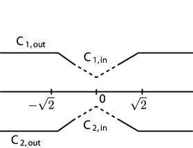
Figure 1: $C_{1}=C_{1,\mathrm{out}}\cup C_{1,\mathrm{in}},\quad C_{2}=C_{2,\mathrm{out}}\cup C_{2,\mathrm{in}}$

Then from Lemma 3.3, $Er(n,z)=O(n^{-2/3})$ for $z\in C_{1}\cup C_{2}$. Also since $\beta(z)=O(1)$, $\beta(z)^{-1}=O(1)$, and $\text{arg}(\beta(z))\in\left(-\frac{\pi}{4},\frac{\pi}{4}\right)$ for $z\in C_{1}\cup C_{2}$, we have $\frac{\beta-\beta^{-1}}{\beta+\beta^{-1}}=O(1)$ for $z\in C_{1}\cup C_{2}$. Thus, we find from (54) that

$$Y_{11}(z)=e^{ng(z)}\frac{\beta(z)+\beta(z)^{-1}}{2}(1+O(n^{-2/3}))$$ (57)

and

$$Y_{21}(z)=e^{ng(z)+nl}\left(O(n^{-2/3})+\frac{\beta(z)-\beta(z)^{-1}}{-2i}(1+O(n^{-2/3}))\right)$$ (58)

for $z\in C_{1}\cup C_{2}$. On the other hand, from the definition (45) of $v_{s}$ and the choice of $C_{1}$ there exists a positive constant $c$ such that

$$\begin{split}v_{s}(z)&=\begin{cases}e^{2i\alpha(z)}(1+O(e^{-cn^{1/6}})),\quad z\in C_{1},\\ e^{-2i\alpha(z)}(1+O(e^{-cn^{1/6}})),\quad z\in C_{2},\end{cases}\end{split}$$ (59)

where $\alpha(z)=\pi(dz+s)=\frac{0pt\sqrt{n}}{\sqrt{2}}z+s\pi$ is defined earlier. Therefore, we find that for $z,w\in C_{1}\cup C_{2}$,

$$K_{s}(z,w)=\frac{f_{1}(z)f_{2}(w)-f_{2}(z)f_{1}(w)}{-2\pi i(z-w)}e^{n\phi(z)+n\phi(w)},$$ (60)

where

$$\phi(z):=\begin{cases}g(z)-\frac{1}{2}z^{2}+\frac{1}{2}l+\frac{i0pt}{\sqrt{2n}}z,\qquad&\textrm{Im}(z)>0,\\ g(z)-\frac{1}{2}z^{2}+\frac{1}{2}l-\frac{i0pt}{\sqrt{2n}}z,\qquad&\textrm{Im}(z)<0,\end{cases}$$ (61)

and $f_{1},f_{2}$ are both analytic in $\mathbb{C}\backslash\mathbb{R}$ and satisfy

$$f_{1}(z)=\begin{cases}e^{is\pi}\frac{\beta(z)+\beta(z)^{-1}}{2}(1+O(n^{-2/3})),\qquad&z\in C_{1},\\ e^{-is\pi}\frac{\beta(z)+\beta(z)^{-1}}{2}(1+O(n^{-2/3})),\qquad&z\in C_{2},\end{cases}$$ (62)

$$f_{2}(z)=\begin{cases}e^{is\pi}\left(O(n^{-2/3})+\frac{\beta(z)-\beta(z)^{-1}}{-2i}(1+O(n^{-2/3}))\right),\qquad&z\in C_{1},\\ e^{-is\pi}\left(O(n^{-2/3})+\frac{\beta(z)-\beta(z)^{-1}}{-2i}(1+O(n^{-2/3}))\right),\qquad&z\in C_{2}.\end{cases}$$ (63)

Note that $f_{1}(z)$, $f_{2}(z)$, and their derivatives are bounded on $C_{1}\cup C_{2}$.

So far we only used the fact that the contours $C_{1}$ and $C_{2}$ satisfy the conditions (56). Now we make a more specific choice of the contours as follows (see Figure 1). For a small fixed $\epsilon>0$ to be chosen in Lemma 3.4, set

$$\Sigma=\{u+iv:\,-\epsilon\leq u\leq\epsilon,\,v=n^{-1/3}+|u|/\sqrt{3}\}.$$ (64)

Define $C_{1,in}$ to be the part of $\Sigma$ such that $|u|\leq n^{-1/4}$:

$$C_{1,\mathrm{in}}=\{u+iv:\,-n^{-1/4}\leq u\leq n^{-1/4},\,v=n^{-1/3}+|u|/\sqrt{3}\}.$$ (65)

Define $C_{1,\mathrm{out}}$ be the union of $\Sigma\setminus C_{1,\mathrm{in}}$ and the horizontal line segments $u+iv_{0}$, $|u|\geq\epsilon$ where $v_{0}$ is the maximal imaginary value of $\Sigma$ given by $v_{0}=n^{-1/3}+\epsilon/\sqrt{2}$. Set $C_{1}=C_{1,\mathrm{in}}\cup C_{1,\mathrm{out}}$. Define $C_{2}=\overline{C_{1}}$. It is clear from the definition that the contours satisfy the conditions (56).

Recall that (see (49)) $0pt=2\sqrt{n}+2^{-2/3}n^{-1/6}x$ where $x\in\mathbb{R}$ is fixed. We have

Lemma 3.4.

There exist $\epsilon>0$, $n_{0}\in\mathbb{N}$, and positive constants $c_{1}$ and $c_{2}$ such that with the definition (64) of $\Sigma$ with this $\epsilon$, $\phi(z)$ defined in (61) satisfies

$$\begin{split}\textrm{Re }\phi(z)\leq c_{1}n^{-1},\qquad&z\in C_{1,\mathrm{in}}\cup C_{2,\mathrm{in}},\\ \textrm{Re }\phi(z)\leq-c_{2}n^{-3/4},\qquad&z\in C_{1,\mathrm{out}}\cup C_{2,\mathrm{out}},\end{split}$$ (66)

for all $n\geq n_{0}$.

Proof.

From the properties of $g(z)$ and $l$, it is easy to show that $g(z)-\frac{1}{2}z^{2}+\frac{1}{2}l=\int_{z}^{\sqrt{2}}\sqrt{s^{2}-2}ds$ for $z\in\mathbb{C}\setminus(-\infty,\sqrt{2}]$ (see e.g. (7.60) [17]). Thus,

$$\phi(z)=\int_{z}^{\sqrt{2}}\sqrt{s^{2}-2}ds\pm\frac{i0pt}{\sqrt{2n}}z,\qquad z\in\mathbb{C}_{\pm}.$$ (67)

This implies that for $\phi_{\pm}(u)$ is purely imaginary for $z=u\in(-\sqrt{2},\sqrt{2})$ where $\phi_{\pm}$ denotes the boundary values from $\mathbb{C}_{\pm}$ respectively. Hence for $u\in(-\sqrt{2},\sqrt{2})$ and $v>0$, $\textrm{Re}\,\phi(u+iv)=\textrm{Re}\,(\phi(u+iv)-\phi_{+}(u))$. For $u^{2}+v^{2}$ small enough and $v>0$, using the Taylor’s series about $s=0$ and also (49), we have

$$\begin{split}\textrm{Re}\,\phi(u+iv)&=-\textrm{Re}\left(\int_{u}^{u+iv}\sqrt{s^{2}-2}ds\right)-\frac{0ptv}{\sqrt{2n}}\\ &=-\frac{1}{2^{3/2}}\textrm{Im}\left(\int_{u}^{u+iv}(s^{2}+O(s^{4}))ds\right)-\frac{x}{2^{7/6}n^{2/3}}v.\end{split}$$ (68)

The integral involving $O(s^{4})$ is $O(|u^{2}+v^{2}|^{5/2})$. On the other hand,

$$-\frac{1}{2^{3/2}}\textrm{Im}\left(\int_{u}^{u+iv}s^{2}ds\right)-\frac{xv}{2^{7/6}n^{2/3}}=-\frac{1}{2^{2/3}3}(3u^{2}v-v^{3})-\frac{xv}{2^{7/6}n^{2/3}}.$$ (69)

For $z=u+iv$ such that $v=n^{-1/3}+|u|/\sqrt{3}$ (see (64)), (69) equals

$$n^{-1}\left(-\frac{2^{7/3}}{3^{5/2}}t^{3}-\frac{2^{1/3}}{3}t^{2}+\frac{(2^{1/2}-x)}{2^{7/6}3^{1/2}}t+\frac{1}{2^{7/6}3}(2^{1/2}-3x)\right),$$ (70)

by setting $t=|u|n^{1/3}$. The polynomial in $t$ is cubic and is of form $f(t)=-a_{1}t^{3}-a_{2}t^{2}+a_{3}t+a_{4}$ where $a_{1},a_{2}>0$ and $a_{3},a_{4}\in\mathbb{R}$. It is easy to check that this function is concave down for positive $t$. Hence

1. $\sup_{t\geq 0}f(t)$ is bounded above and

2. there are $c>0$ and $t_{0}>0$ such that $f(t)\leq-ct^{3}$ for $t>t_{0}$.

Note that for $z\in C_{1,\mathrm{in}}$, $t\in[0,n^{1/12}]$. Using $(i)$, we find that (70) is bounded above by a constant time $n^{-1}$ for uniformly in $z\in C_{1,\mathrm{in}}$. Since the integral involving $O(s^{4})$ in (68) is $O(n^{-5/4})$ when $z\in C_{1,\mathrm{in}}$, we find that there is a constant $c_{1}>0$ such that $\textrm{Re}\,\phi(z)\leq c_{1}n^{-1}$ for $z\in C_{1,\mathrm{in}}$.

Now, for $z=u+iv$ such that $v=n^{-1/3}+|u|/\sqrt{3}$ and $|u|\geq n^{-1/4}$, we have $t=|u|n^{1/3}\geq n^{1/12}$ and hence from (ii),  (70) is bounded above by $-ct^{3}n^{-1}=-c|u|^{3}$ for all large enough $n$. On the other hand, for such $z$, the integral involving $O(s^{4})$ in (68) is $O(|z|^{5})=O(|u|^{5})$. Hence $\textrm{Re}\,\phi(z)\leq-c|u|^{3}+O(|u|^{5})$ for such $z$. Now if we take $\epsilon>0$ small enough, then there is $c_{2}>0$ such that $\textrm{Re}\,\phi(z)\leq-c_{2}|u|^{3}$ for $|u|\leq\epsilon$. Combining this, we find that there exist $\epsilon>0$, $n_{0}\in\mathbb{N}$, and $c_{2}>0$ such that for $\Sigma$ with this $\epsilon$, we have $\textrm{Re}\,\phi(z)\leq-c_{2}|u|^{3}$ for $z=u+iv\in\Sigma\setminus C_{1,\mathrm{in}}$. Since $|u|\geq n^{-1/4}$ for such $z$, we find $\textrm{Re}\,\phi(z)\leq-c_{2}n^{-3/4}$ for $z\in\Sigma\setminus C_{1,\mathrm{in}}$.

We now fix $\epsilon$ as above and consider the horizontal part of $C_{1,\mathrm{out}}$. Note that from (67), for fixed $v_{0}>0$,

$$\begin{split}\frac{\partial}{\partial u}\text{Re}\,\phi(u+iv_{0})=\text{Re}\,\phi^{\prime}(u+iv_{0})=-\text{Re}\,\sqrt{(u+iv_{0})^{2}-2}.\end{split}$$ (71)

It is straightforward to check that this is $<0$ for $u>0$ and $>0$ for $u<0$. Hence the value of $\text{Re}\,\phi(z)$ for $z$ on the horizontal part of $C_{1,\mathrm{out}}$ is the largest at the end which are the intersection points of the horizontal segments and $\Sigma$. Since $\textrm{Re}\,\phi(z)\leq-c_{2}n^{-3/4}$ for $z\in\Sigma\setminus C_{1,\mathrm{in}}$, we find that the same bound holds for all $z$ on the horizontal segments of $C_{1,\mathrm{out}}$. Therefore, we obtain $\textrm{Re }\phi(z)\leq-c_{2}n^{-3/4}$ for all $z\in C_{1,\mathrm{out}}$.

The estimates on $C_{2}$ follows from the estimates on $C_{1}$ due to the symmetry of $\phi$ about the real axis. ∎

Inserting the estimates in Lemma 3.4 to the formula (60) and using the fact that $f_{j}(z)$, $j=1,2$, and their derivatives are bounded on $C_{1}\cup C_{2}$ (see (62) and (63)), we find that

$$K_{s}(z,w)\leq O(e^{-c_{2}n^{1/4}}),\qquad\text{if one of $z$ or $w$ is in $C_{1,\mathrm{out}}\cup C_{2,\mathrm{out}}$.}$$ (72)

We now analyze the kernel $K_{s}(z,w)$ when $z,w\in C_{1,\mathrm{in}}\cup C_{2,\mathrm{in}}$. We first scale the kernel. Set

$$\hat{K}_{s}(\xi,\eta):=2\pi i\cdot i2^{1/6}n^{-1/3}K_{s}(i2^{1/6}n^{-1/3}\xi,i2^{1/6}n^{-1/3}\eta).$$ (73)

We also set

$$\begin{split}\Sigma_{1}^{(n)}:=\left\{u+iv:\,u=2^{-1/6}+3^{-1/2}|v|,\,-2^{-1/6}n^{1/12}\leq v\leq 2^{-1/6}n^{1/12}\right\}.\end{split}$$ (74)

This contour is oriented from top to bottom. Note that if $\zeta\in\Sigma_{1}^{(n)}$, then

$$z=i2^{1/6}n^{-1/3}\zeta\in C_{1,\mathrm{in}}.$$ (75)

We also set $\Sigma_{2}^{(n)}=\{-\xi:\xi\in\Sigma_{1}^{(n)}\}$ with the orientation from top to bottom. Then

$$\det(1+K_{s})_{L^{2}(C_{1,in}\cup C_{2,in},dz)}=\det(1+\hat{K}_{s})_{L^{2}(\Sigma_{1}^{(n)}\cup\Sigma_{2}^{(n)},\frac{d\zeta}{2\pi i})}.$$ (76)

From (67),

$$\phi(z)=\begin{cases}\frac{\pi i}{2}+\left(\frac{0pt-2\sqrt{n}}{\sqrt{2n}}\right)iz+2^{-3/2}3^{-1}iz^{3}+O(z^{5}),\quad&z\in C_{1,\mathrm{in}},\\ -\frac{\pi i}{2}-\left(\frac{0pt-2\sqrt{n}}{\sqrt{2n}}\right)iz-2^{-3/2}3^{-1}iz^{3}+O(z^{5}),\quad&z\in C_{2,\mathrm{in}}.\end{cases}$$ (77)

This implies that, using (49) and $|z|=O(n^{-1/4})$ for $z\in C_{1,\mathrm{in}}\cup C_{2,\mathrm{in}}$,

$$n\phi(i2^{1/6}n^{-1/3}\zeta)=\begin{cases}\frac{n\pi i}{2}+m_{x}(\zeta)+O(n^{-1/4}),\qquad&\zeta\in\Sigma_{1}^{(n)},\\ -\frac{n\pi i}{2}-m_{x}(\zeta)+O(n^{-1/4}),\qquad&\zeta\in\Sigma_{2}^{(n)},\end{cases}$$ (78)

where

$$m_{x}(\zeta):=-\frac{1}{2}x\zeta+\frac{1}{6}\zeta^{3},\qquad\zeta\in\mathbb{C}.$$ (79)

It is also easy to check from the definition (53) that

$$\beta(i2^{\frac{1}{6}}n^{-\frac{1}{3}}\zeta)=\begin{cases}e^{\frac{i\pi}{4}}\left(1-i2^{-\frac{4}{3}}n^{-\frac{1}{3}}\zeta+O(n^{-\frac{1}{2}})\right),\qquad&\zeta\in\Sigma_{1}^{(n)},\\ e^{\frac{-i\pi}{4}}\left(1-i2^{-\frac{4}{3}}n^{-\frac{1}{3}}\zeta+O(n^{-\frac{1}{2}})\right),\qquad&\zeta\in\Sigma_{2}^{(n)}.\end{cases}$$ (80)

Using these we now evaluate (73). Set

$$z=i2^{1/6}n^{-1/3}\xi,\qquad w=i2^{1/6}n^{-1/3}\eta.$$ (81)

We consider two cases separately: (a) $z,w\in C_{1,\mathrm{in}}$ or $z,w\in C_{2,\mathrm{in}}$, and (b) $z\in C_{1,\mathrm{in}},w\in C_{2,\mathrm{in}}$, or $z\in C_{2,\mathrm{in}},w\in C_{1,\mathrm{in}}$. From (80),

$$\begin{split}\frac{\beta(z)-\beta(w)}{z-w}=O(1)\qquad\text{for case (a),}\end{split}$$ (82)

and

$$\begin{split}\frac{\beta(z)-\beta(w)}{z-w}=\pm n^{1/3}\frac{2^{5/6}\sin\frac{\pi}{4}}{\xi-\eta}(1+O(n^{-\frac{1}{4}}))\quad\text{for case (b).}\end{split}$$ (83)

Here the sign is $+$ when $z\in C_{1,\mathrm{in}},w\in C_{2,\mathrm{in}}$ and $-$ when $z\in C_{2,\mathrm{in}},w\in C_{1,\mathrm{in}}$. We also note that using (80), for $z\in C_{1,\mathrm{in}}\cup C_{2,\mathrm{in}}$ the asymptotic formula (63) can be expressed as

$$f_{2}(z)=\begin{cases}e^{is\pi}\frac{\beta(z)-\beta(z)^{-1}}{-2i}\left(1+O(n^{-5/12})\right),\qquad&z\in C_{1,\mathrm{in}},\\ e^{-is\pi}\frac{\beta(z)-\beta(z)^{-1}}{-2i}\left(1+O(n^{-5/12})\right),\qquad&z\in C_{2,\mathrm{in}}.\end{cases}$$ (84)

Thus, (62), (80), and (83), implies that for case (b),

$$\begin{split}\frac{f_{1}(z)f_{2}(w)-f_{1}(z)f_{2}(w)}{-2\pi i(z-w)}=&-(\beta(z)^{-1}+\beta(w)^{-1})\frac{\beta(z)-\beta(w)}{4\pi(z-w)}\left(1+O(n^{-5/12})\right)\\ =&\mp n^{1/3}\frac{\cos(\frac{\pi}{4})\sin(\frac{\pi}{4})}{2^{1/6}\pi(\xi-\eta)}(1+O(n^{-\frac{1}{4}})).\end{split}$$ (85)

Inserting this and (78) into (60) (recall (73)), we find that

$$\hat{K}_{s}(\xi,\eta)=\pm\frac{e^{\pm(m_{x}(\xi)-m_{x}(\eta))}}{\xi-\eta}(1+O(n^{-1/4})),$$ (86)

for case (b). A similar calculation using (82) instead of (83) implies that $\hat{K}_{s}(\xi,\eta)=O(n^{-1/3})$ for case (a).

The above calculations imply that $\hat{K}_{s}$ converges to the operator given by the leading term in (87) or $0$ depending on whether $\xi$ and $\eta$ are on different limiting contours or on the same limiting contours. From this structure, we find that $\hat{K}_{s}$ converges to $\big{(}\begin{smallmatrix}0&K_{12}^{(\infty)}\\ K_{21}^{(\infty)}&0\end{smallmatrix}\big{)}$ on $L^{2}(\Sigma^{(\infty)}_{1},\frac{d\zeta}{2\pi i})\oplus L^{2}(\Sigma^{(\infty)}_{2},\frac{d\zeta}{2\pi i})$ in the sense of pointwise limit of the kernel where

$$K_{12}^{(\infty)}(\xi,\eta)=\frac{e^{m_{x}(\xi)-m_{x}(\eta)}}{\xi-\eta},\quad K_{21}^{(\infty)}(\xi,\eta)=-\frac{e^{-(m_{x}(\xi)-m_{x}(\eta))}}{\xi-\eta},$$ (87)

and $\Sigma^{(\infty)}_{1}$ is a simple contour from $e^{i\pi/3}\infty$ to $e^{-i\pi/3}\infty$ staying in the right half plane, and $\Sigma^{(\infty)}_{2}=-\Sigma^{(\infty)}_{1}$ from $e^{2\pi i/3}\infty$ to $e^{-2\pi i/3}\infty$. Note that the limiting kernel does not depend on $s$.

In order to ensure that the Fredholm determinant also converges to the Fredholm determinant of the limiting operator, we need additional estimates for the derivatives to establish the convergence in trace norm. It is not difficult to check that the formal derivatives of the limiting operators indeed yields the correct limits of the derivatives of the kernel. We do not provide the details of these estimates since the arguments are similar and the calculation follows the standard argument. Then we obtain

$$\lim_{n\rightarrow\infty}\det\left.\big{(}1+\hat{K}_{s}\big{)}\right|_{L^{2}(\Sigma_{1}^{(n)}\cup\Sigma_{2}^{(n)},\frac{d\zeta}{2\pi i})}=\det\left.\big{(}1-K^{(\infty)}_{x}\big{)}\right|_{L^{2}(\Sigma_{1}^{(\infty)},\frac{d\zeta}{2\pi i})},$$ (88)

where $K^{(\infty)}_{x}=K_{12}^{(\infty)}K_{21}^{(\infty)}$ of which the kernel is

$$K^{(\infty)}_{x}(\xi,\eta):=e^{m_{x}(\xi)+m_{x}(\eta)}\int_{\Sigma^{(\infty)}_{2}}\frac{e^{-2m_{x}(\zeta)}}{(\xi-\zeta)(\eta-\zeta)}\frac{d\zeta}{2\pi i}.$$ (89)

The determinant $\det(1-K^{(\infty)}_{x})$ equals the Fredholm determinant of the Airy operator. Indeed, this determinant is a conjugated version of the determinant in the paper [38] on ASEP. If we call the operator in (33) of [38] $L_{s}(\eta,\eta^{\prime})$, then $K^{(\infty)}_{x}(\xi,\eta)=e^{m_{x}(\xi)}L_{x}(\xi,\eta)e^{-m_{x}(\eta)}$. It was shown in page 153 in [38] that $\det(1+L_{s})=\det(1-K_{Airy})_{(s,\infty)}=F(s)$.

Now, since $\lim_{n\to\infty}P_{s}(M)=\lim_{n\to\infty}\det(1+K)_{L^{2}(C_{+}\cup C_{-})}$ by (72),  (76) and (88) implies that $P_{s}(2\sqrt{n}+2^{-\frac{2}{3}}n^{-\frac{1}{6}}x)\rightarrow F(x)$ for all $s$. All the estimates are uniform in $s\in[0,1]$ and we obtain $\mathbb{P}\left(W_{n}<2\sqrt{n}+2^{-2/3}n^{-1/6}x\right)=\int_{0}^{1}P_{s}(M)ds\to F(x)$. This proves Theorem 1.2.

4 Symmetric simple random walks

4.1 Continuous-time symmetric simple random walks

Let $Y(t)$ be a continuous-time symmetric simple random walk. This can also be thought of as the difference of two independent rate $1/2$ Poisson processes. The transition probability is given by $p_{t}(x,y)=p_{t}(y-x)$ where

$$p_{t}(k)=e^{-t}\sum_{n\in\mathbb{Z}}\frac{(t/2)^{2n+k}}{n!(n+k)!},\qquad k\in\mathbb{Z}.$$ (90)

where $\frac{1}{k!}:=0$ for $k<0$ by definition. Let $Y_{i}(t)$ be independent copies of $Y$ and set $X_{i}(t)=Y_{i}(t)+i$, $i=0,1,2,\cdots,n-1$. Also set $X(t):=(X_{0}(t),X_{1}(t),\cdots,X_{n-1}(t))$. Then $X(0)=\left(0,1,\cdots,n-1\right)$. We condition on the event that (a) $X(T)=X(0)$ and (b) $X_{0}(t)<X_{1}(t)<\cdots<X_{n-1}(t)$ for all $t\in[0,T]$. See, for example, [2]. We use the notation $\mathbb{P}$ to denote this conditional probability.

Define the ‘width’ as

$$W_{n}(T)=\sup_{t\in[0,T]}(X_{n-1}(t)-X_{1}(t)).$$ (91)

The analogue of Proposition 1.1 is the following. The proof is given at the end of this section.

Proposition 4.1.

For non-intersecting continuous-time symmetric simple random walks,

$$\mathbb{P}(W_{n}(T)<0pt)=\frac{1}{\mathcal{T}_{n}(f)}\oint_{|s|=1}\mathbf{T}_{n}(f,\mathcal{D}_{s})\frac{ds}{2\pi is},\quad f(z)=e^{\frac{T}{2}(z+z^{-1})},$$ (92)

and $\mathcal{D}_{s}=\{z\in\mathbb{C}:z^{M}=s\}$.

The limit theorem is:

Theorem 4.1.

For each $x\in\mathbb{R}$,

$$\lim_{\min\{n,T\}\to\infty}\mathbb{P}\left(\frac{W_{n}(T)-\mu(n,T)}{\sigma(n,T)}\leq x\right)=F(x)$$ (93)

where

$$\mu(n,T):=\begin{cases}2\sqrt{nT},\qquad&n<T,\\ n+T,\qquad&n\geq T,\end{cases}$$ (94)

and

$$\sigma(n,T):=\begin{cases}2^{-2/3}T^{1/3}\big{(}\sqrt{\frac{n}{T}}+\sqrt{\frac{T}{n}}\big{)}^{1/3},\quad&n<T,\\ 2^{-1/3}T^{1/3},\quad&n\geq T.\end{cases}$$ (95)

Note that due to the initial condition and the fact that at most one of $X_{j}$’s moves with probability $1$ at any given time, if $X_{i}$ is to move downward at time $t$, it is necessary that $X_{0},\cdots,X_{i-1}$ should have moved downward at least once during the time interval $[0,t)$. Thus, if $T$ is small compared to $n$, then only a few bottom walkers can move downard (and similarly, only a few top walkers can move upward), and hence the middle walkers are ‘frozen’(See Figure 2). On the other hand, if $T$ is large compared to $n$, then there is no frozen region. The above result shows that the transition occurs when $T=n$ at which point the scalings (94) and (95) change.

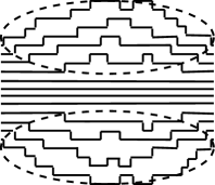
Figure 2: Frozen region when $T<n$

Using Theorem 1.1, Theorem 4.1 can be obtained following the similar analysis as in Section 3.2 once we have the asymptotics of the (continuous) orthonormal polynomials with respect to the measure $e^{\frac{T}{2}(z+z^{-1})}\frac{dz}{2\pi iz}$ on the unit circle. The asymptotics of these particular orthonormal polynomials were studied in [6] and [5] using the Deift-Zhou steepest-descent analysis of Riemann-Hilbert problems. In order to be able to control the operator (5), the estimates on the error terms in the asymptotics need to be improved. It is not difficult to achieve such estimates by keeping track of the error terms more carefully in the analysis of [6] and [5]. We do not provide any details. Instead we only comment that the difference of the scalings for $n<T$ and $n>T$ is natural from the Riemann-Hilbert analysis of the orthonormal polynomials. If we consider the orthonormal polynomial of degree $n$, $p_{n}(z)$, with weight $e^{\frac{T}{2}(z+z^{-1})}$, the support of the equilibrium measure changes from the full circle when $\frac{n}{T}>1$ to an arc when $\frac{n}{T}<1$. The “gap” in the support starts to appear at the point $z=-1$ when $n=T$ and grows as $\frac{n}{T}$ decreases. This results in different asymptotic formulas of the orthonormal polynomials in two different regimes of parameters. However, we point out that the main contribution to the kernel (5) turns out to come from the other point on the circle, namely $z=1$.

For technical reasons, the Riemann-Hilbert analysis is done separately for the following four overlapping regimes of the parameters: (I) $n\geq T+C_{1}T^{1/3}$, (II) $T-C_{2}T^{1/3}\leq n\leq T+C_{3}T^{1/3}$, (III) $c_{1}T\leq n\leq T-C_{4}T^{1/3}$, (IV) $n\leq c_{2}T$ where $0<c_{k}<1$ and $C_{k}>0$.

Here we only indicate how the leading order calculation leads to the GUE Tracy-Widom distribution for the case (I). We take

$$M=n+T+2^{-1/3}T^{1/3}x.$$ (96)

Let $p_{n}(z)$ be the orthonormal polynomial and $\kappa_{n}$ be its leading coefficient. For case (I), the Riemann-Hilbert analysis implies that

$$\kappa_{n}^{-1}p_{n}(z)\approx\begin{cases}z^{n}e^{-\frac{T}{2}z^{-1}},\qquad&|z|>1,\\ o(e^{-\frac{T}{2}z}),\qquad&|z|<1,\end{cases}$$ (97)

and

$$\kappa_{n}p_{n}^{*}(z)\approx\begin{cases}o(z^{n}e^{-\frac{T}{2}z^{-1}}),\qquad&|z|>1,\\ e^{-\frac{T}{2}z},\qquad&|z|<1.\end{cases}$$ (98)

Here these asymptotics can be made uniform for $|z-1|\geq O(T^{-1/3})$. In the below, we always assume that $z$ and $w$ satisfy this condition even if we do not state it explicitly. The above estimates imply that the leading order of $z^{n/2}K_{conti}w^{-n/2}$, where $K_{conti}$ is defined in (6), becomes

$$z^{n/2}K_{conti}(z,w)w^{-n/2}\approx\begin{cases}z^{n/2}\frac{e^{-\frac{T}{2}(z^{-1}+w)}}{1-z^{-1}w}w^{-n/2},\quad&|z|>1,\,|w|<1,\\ -z^{-n/2}\frac{e^{-\frac{T}{2}(z+w^{-1})}}{1-z^{-1}w}w^{n/2},\quad&|z|<1,\,|w|>1.\end{cases}$$ (99)

The kernel is of smaller order than the above when $|z|<1,|w|<1$ or $|z|>1,|w|>1$. Since $\mathcal{D}=\mathcal{D}_{s}=\{z\in\mathbb{C}:z^{M}=s\}$, we choose $\gamma(z)=z^{M}-s$ and

$$v(z):=\begin{cases}\frac{s}{z^{M}-s}\approx sz^{-M},\quad&|z|>1,\\ \frac{z^{M}}{s-z^{M}}\approx\frac{1}{s}z^{M},\quad&|z|<1.\end{cases}$$ (100)

Here again the approximation is uniform for $|z-1|\geq O(T^{-1/3})$. Hence inserting $f(z)=e^{\frac{T}{2}(z+z^{-1})}$, we find that the leading order term of (5) is

$$z^{n/2}K(z,w)w^{-n/2}\approx\pm\frac{e^{\pm(\phi(z)-\phi(w)})}{1-z^{-1}w},\quad\phi(z):=\frac{T}{4}(z-z^{-1})-\frac{M-n}{2}\log z$$ (101)

where the sign is $+$ is when $|z|>1,|w|<1$ and is $-$ when $|z|<1,|w|>1$. Using (96), we note that

$$\phi(z)=-\frac{T^{1/3}}{2^{4/3}}x(z-1)+\frac{T}{12}(z-1)^{3}+O(T^{1/3}(z-1)^{2})+O(T(z-1)^{4}).$$ (102)

Hence for $\zeta=O(1)$,

$$\phi(1+\frac{2^{1/3}}{T^{1/3}}\zeta)=-\frac{1}{2}x\zeta+\frac{1}{6}\zeta^{3}+O(T^{-1/3}).$$ (103)

After the scaling $z=1+\frac{2^{1/3}}{T^{1/3}}\zeta$ and $w=1+\frac{2^{1/3}}{T^{1/3}}\eta$, (101) converges to the leading term of (87), except for the overall sign change which is due to the reverse orientation of the contour. Thus we end up with the same limit (88) which is $F(x)$.

Proof of Proposition 4.1.

Similarly to Lemma 3.1 we apply the Karlin-McGregor argument in the chamber $\{x_{0}<x_{1}<\cdots<x_{n-1}<x_{0}+0pt\}$ and obtain that

$$\mathbb{P}\left(W_{n}(T)<0pt\right)=\frac{\sum_{h_{j}\in\mathbb{Z},h_{0}+h_{1}+\cdots+h_{n-1}=0}\det\left[p_{T}(x_{j}-y_{k}+h_{k}0pt)\right]_{j,k=0}^{n-1}}{\det\left[p_{T}(x_{j}-y_{k})\right]_{j,k=0}^{n-1}}.$$ (104)

Note that numerator equals

$$\oint_{|s|=1}\det\left[\sum_{h\in\mathbb{Z}}p_{T}(x_{j}-y_{k}+h0pt)s^{h}\right]_{j,k=0}^{n-1}\frac{ds}{2\pi is}.$$ (105)

Since (90) can be written as

$$p_{T}(x)=e^{-T}\oint_{|z|=1}z^{-x}e^{\frac{T}{2}(z+z^{-1})}\frac{dz}{2\pi iz},$$ (106)

we find that

$$\sum_{h\in\mathbb{Z}}p_{T}(x+h0pt)s^{h}=\frac{e^{-T}}{0pt}\sum_{z^{0}pt=s}z^{-x}e^{\frac{T}{2}(z+z^{-1})}.$$ (107)

Proposition 4.1 follows immediately. ∎

Remark 4.1.

If we were to evaluate the ratio $\frac{\mathbf{T}_{n}(f,\mathcal{D}_{s})}{\mathcal{T}_{n}(f)}$ directly instead of using the Fredholm determinant formula, we need to find the asymptotic expansion of the log of the determinants to the order $o(1)$ including the constant term. This is relatively easy to obtain for $\mathcal{T}_{n}(f)$ when $\frac{T}{n}<1$: the Szegö limit theorem essentially applies with an exponentially decaying error term. However, when $\frac{T}{n}>1$, this calculation is cumbersome and complicated [6], and the asymptotic expansions had not been obtained to the desired order . Especially, the determination of the constant term in the asymptotic expansion would require some sophisticated analysis (see e.g. [18, 5]). The difficulty is due to the following fact that the orthogonal polynomials only give the asymptotics of the ratio $\mathcal{T}_{k}(f)/\mathcal{T}_{k-1}(f)$, whose error terms are of exponential type when $\frac{T}{n}<1$ but are of polynomial type when $\frac{T}{n}>1$. This technicality is also directly related to the difficulty in obtaining the precise asymptotic in the lower tail regime for the length of the longest increasing subsequences or other directed last passage percolation models [6, 7]. For $f$ above, it turns out that the discrete Toeplitz determinant $\mathbf{T}_{n}(f,\mathcal{D}_{m})$ essentially factors into two parts asymptotically, one of which is same as the asymptotic of the continuous Toeplitz determinant [8]. The formula (4) is precisely of the form that this cancellation is already taken into account. By this reason, we could evaluate the limit of $\frac{\mathbf{T}_{n}(f,\mathcal{D}_{s})}{\mathcal{T}_{n}(f)}$ for certain $m$ even if we do not have the asymptotic formula of each determinant to the order $o(1)$. We note that the asymptotic evaluation of the Fredholm determinant may become difficult for other choices of $m$, especially for those which correspond to the so-called ‘saturated region’ conditions for the discrete orthogonal polynomials.

4.2 Discrete-time symmetric simple random walks

Let $X_{0}(k),\cdots,X_{n-1}(k)$, $k=0,1,\cdots,n-1$, be independent discrete-time symmetric simple random walks. Set $X(k):=(X_{0}(k),X_{1}(k),\cdots,X_{n-1}(k))$. We take the initial condition as

$$X(0)=(0,2,\cdots,2n-2).$$ (108)

and consider the process conditional of the event that (a) $X(2T)=X(0)$ and (b) $X_{0}(k)<X_{1}(k)<\cdots<X_{n-1}(k)$ for all $k=0,1,\cdots,2T$. The non-intersecting discrete-time simple random walks can also be interpreted as random tiling of a hexagon and were studied in many papers. See, for example, [13, 26, 9, 11]. The notation $\mathbb{P}$ denotes this conditional probability. Define the width $W_{n}(2T):=\max_{k=0,1,\cdots,2T}\big{(}X_{n-1}(k)-X_{0}(k)\big{)}$ as before.

Proposition 4.2.

For non-intersecting discrete-time symmetric simple random walks,

$$\mathbb{P}(W_{n}(2T)<20pt)=\frac{1}{\mathcal{T}_{n}(f)}\oint_{|s|=1}\mathbf{T}_{n}(f,\mathcal{D}_{s})\frac{ds}{2\pi is},\quad f(z)=z^{-T}(1+z)^{2T},$$ (109)

and $\mathcal{D}_{s}=\{z\in\mathbb{C}:z^{M}=s\}$.

The fluctuations are again given by $F$. Note that $2n\leq W_{n}(2T)\leq 2n+2T$ for all $n$ and $T$.

Theorem 4.2.

Fix $\gamma>0$ and $0<\beta<2$. Then for $n=[\gamma T^{\beta}]$,

$$\lim_{T\to\infty}\mathbb{P}\left(\frac{W_{n}(2T)-2\sqrt{n^{2}+2nT}}{(n^{2}+2nT)^{-\frac{1}{6}}T^{\frac{2}{3}}}\leq x\right)=F(x).$$ (110)

for each $x\in\mathbb{R}$.

Note that the parameter $(n^{2}+2nT)^{-\frac{1}{6}}T^{\frac{2}{3}}\to\infty$ as $T\to\infty$ when $\beta<2$. This parameter is $O(1)$ when $\beta=2$. Indeed one can show that when $\beta>2$,

$$\lim_{T\to\infty}\mathbb{P}(W_{n}(2T)=2n+2T)=1.$$ (111)

The proofs of the proposition and the theorem are similar to those for the continuous-time symmetric simple random walks and we omit them.

5 Proof of Theorem 1.3

In this section we give a proof of Theorem 1.3. The proof is based on the results on a solvable directed last passage percolation model and is similar to the proof of the identity (21) by Johansson [27].

By symmetry we may assume $\alpha\leq\beta$. Let $w(i,j),(i,j)\in\mathbb{N}^{2},$ be independent random variables with geometric distribution, $\mathbb{P}(w(i,j)=k)=(1-q)q^{k}$, $k=0,1,2,\cdots$. Define the random variable (point-to-point directed last passage time)

$$G(M,N)=\max_{\pi}\bigg{(}\sum_{(i,j)\in\pi}w(i,j)\bigg{)},$$ (112)

where the maximum is taken over all possible up/right paths from $(1,1)$ to $(M,N)$. The limiting fluctuations of $G(M,N)$ are known to be $F$ in [25] as $M$ and $N$ tend to infinite with a finite ratio. In particular, when $M=N=(\alpha+\beta)n$,

$$\lim_{n\rightarrow\infty}\mathbb{P}\left(\frac{G((\alpha+\beta)n,(\alpha+\beta)n)-\mu(\alpha+\beta)n}{\sigma(\alpha+\beta)^{1/3}n^{1/3}}\leq s\right)=F(s),$$ (113)

where

$$\mu=\frac{2\sqrt{q}}{1-\sqrt{q}},\qquad\sigma=\frac{q^{1/6}(1+\sqrt{q})^{1/3}}{1-\sqrt{q}}.$$ (114)

Consider the lattice points on the line connecting the points $(1,2\alpha n)$ and $(2\alpha n,1)$, i.e. $\mathcal{L}:=\{(\alpha n+u,\alpha n-u):|u|<\alpha n\}$. An up/right path from $(1,1)$ to $((\alpha+\beta)n,(\alpha+\beta)n)$ passes through a point on $\mathcal{L}$. Considering the up/right path from $(1,1)$ to a point on $\mathcal{L}$ and the down/left path from $((\alpha+\beta)n,(\alpha+\beta)n)$ to the same point on $\mathcal{L}$ (see Figure 3), we find that $G((\alpha+\beta)n,(\alpha+\beta)n)$ equals

$$\max_{|u|<\alpha n}\left(G^{(1)}(\alpha n+u,\alpha n-u)+G^{(2)}(\beta n+u,\beta n-u)\right)+O(1),$$ (115)

where $G^{(1)}$ and $G^{(2)}$ are two independent copies of $G$, and the error term $O(1)$ comes from the duplicate diagonal term $w(\alpha n+u,\alpha n-u)$.

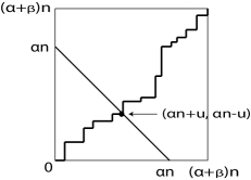
Figure 3: Intersection of an up/right path with $\mathcal{L}$

Consider $G^{(i)}(\alpha n+u,\alpha n-u)$ as a process in time $u$. For $u$ of order $n^{2/3}$, it was shown in [27] that the fluctuations of this process converge the Airy process in the functional convergence. More precisely, if we set

$$H^{(1)}_{n}(\tau):=\frac{G^{(1)}(\alpha n+d^{-1}(\alpha n)^{2/3}\tau,\alpha n-d^{-1}(\alpha n)^{2/3}\tau)-\mu\alpha n}{\sigma(\alpha n)^{1/3}},$$ (116)

and

$$H^{(2)}_{n}(\tau):=\frac{G^{(2)}(\beta n+d^{-1}(\beta n)^{2/3}\tau,\beta n-d^{-1}(\beta n)^{2/3}\tau)-\mu\beta n}{\sigma(\beta n)^{1/3}},$$ (117)

for $|\tau|<d(\alpha n)^{1/3}$, where $d:=q^{1/6}(1+\sqrt{q})^{-2/3}$, then $H^{(i)}_{n}(\tau)$ converges to the Airy process $\mathcal{A}^{(i)}(\tau)-\tau^{2}$, $i=1,2$. (We note that there is a typographical error in the formula (1.8) in [27] where, in terms of our notations, $\sigma$ is changed to $\frac{q^{1/6}(1+\sqrt{q})^{1/3}}{1-q}$. However, the correct formula of $\sigma$ is $\frac{q^{1/6}(1+\sqrt{q})^{1/3}}{1-\sqrt{q}}$ as in (114) which is also same as in [25].) Since (115) implies that

$$\begin{split}&\mathbb{P}\left(\frac{G(N,N)-\mu N}{\sigma N^{1/3}}\leq s\right)\\ &=\mathbb{P}\left(\max_{|\tau|<d\alpha n^{1/3}}\left(\alpha^{1/3}H_{n}^{(1)}(\alpha^{-2/3}\tau)+\beta^{1/3}H_{n}^{(2)}(\beta^{-2/3}\tau)\right)\leq(\alpha+\beta)^{1/3}s\right)+O(N^{-1/3}),\end{split}$$ (118)

we obtain Theorem 1.3 if we prove that

$$\begin{split}&\lim_{n\to\infty}\mathbb{P}\left(\max_{|\tau|<d\alpha n^{1/3}}\left(\alpha^{1/3}H_{n}^{(1)}(\alpha^{-2/3}\tau)+\beta^{1/3}H_{n}^{(2)}(\beta^{-2/3}\tau)\right)\leq(\alpha+\beta)^{1/3}s\right)\\ &=\mathbb{P}\left(\max_{\tau\in\mathbb{R}}\left(\alpha^{1/3}\mathcal{A}^{(1)}(\alpha^{-2/3}\tau)+\beta^{1/3}\mathcal{A}^{(2)}(\beta^{-2/3}\tau)-(\alpha^{-1}+\beta^{-1})\tau^{2}\right)\leq(\alpha+\beta)^{1/3}s\right).\end{split}$$ (119)

In [27], a similar identity

$$\lim_{n\to\infty}\mathbb{P}\left(\max_{|\tau|<dn^{1/3}}H_{n}(\tau)\leq s\right)=\mathbb{P}\left(\max_{\tau\in\mathbb{R}}(\mathcal{A}(\tau)-\tau^{2})\leq s\right)$$ (120)

was proved as a part of the proof of (21). We proceed similarly and use the estimates obtained in [27] .

Set

$$\begin{split}X_{n,T}:=(\alpha+\beta)^{-1/3}\cdot\max_{|\tau|\leq T}\left(\alpha^{1/3}H_{n}^{(1)}(\alpha^{-2/3}\tau)+\beta^{1/3}H_{n}^{(2)}(\beta^{-2/3}\tau)\right)\end{split}$$ (121)

and

$$\begin{split}Y_{n,T}:=(\alpha+\beta)^{-1/3}\cdot\max_{|\tau|>T}\left(\alpha^{1/3}H_{n}^{(1)}(\alpha^{-2/3}\tau)+\beta^{1/3}H_{n}^{(2)}(\beta^{-2/3}\tau)\right).\end{split}$$ (122)

Since

$$\begin{split}&\mathbb{P}(X_{n,T}\leq s)\\ &\geq\mathbb{P}\left(\max_{|\tau|<d\alpha n^{1/3}}\left(\alpha^{1/3}H^{(1)}(\alpha^{-2/3}\tau)+\beta^{1/3}H_{n}^{(2)}(\beta^{-2/3}\tau)\right)\leq(\alpha+\beta)^{1/3}s\right)\\ &\geq\mathbb{P}(X_{n,T}\leq s)-\mathbb{P}(Y_{n,T}>s)\end{split}$$ (123)

for all large enough $n$ for each fixed $T$, (119) follows from the following three properties:

1. For each $\epsilon>0$, there are positive constants $T_{0}$ and $n_{0}$ such that $\mathbb{P}\left(Y_{n,T}>s\right)<\epsilon$ for all $T>T_{0}$ and $n>n_{0}$,

2. For each fixed $T$, $\mathbb{P}\left(X_{n,T}\leq s\right)\to\mathbb{P}\left(A_{T}\leq s\right)$ as $n\to\infty$.

3. Finally, $\mathbb{P}(A_{T}\leq s)\to\mathbb{P}(A_{\infty}\leq s)$ as $T\to\infty$.

Here

$$\begin{split}A_{T}:=(\alpha+\beta)^{-1/3}\cdot\max_{|\tau|\leq T}\left(\alpha^{1/3}\mathcal{A}^{(1)}(\alpha^{-2/3}\tau)+\beta^{1/3}\mathcal{A}^{(2)}(\beta^{-2/3}\tau)-(\alpha^{-1}+\beta^{-1})\tau^{2}\right)\end{split}$$ (124)

and $A_{\infty}$ is the same random variable with the maximum taken over $\tau\in\mathbb{R}$.

A functional limit theorem to the Airy process was proved in [27] (Theorem 1.2). This means that $H_{n}^{(i)}(\tau)\to\mathcal{A}^{(i)}(\tau)-\tau^{2}$ at $n\to\infty$ in the sense of weak convergence of the probability measures on $C[-T,T]$ for each fixed $T$. Hence the property (b) follows a theorem on the convergence of product measures ([10], Theorem 3.2).

The property (c) follows from the monotone convergence theorem since $\{A_{\infty}\leq s\}=\cap_{T>0}\{A_{T}\leq s\}$.

For the property (a), we use the estimates (5.19) and (5.20) in [27]: there are positive constants $C$ and $c$ such that

$$\begin{split}&\mathbb{P}\left(\max_{T<\tau\leq\log n}H_{n}^{(i)}(\alpha^{-2/3}\tau)>M\right)\\ &\leq\int_{\alpha^{-2/3}T-1}^{\infty}e^{-c(M-1+x^{2})^{3/2}}dx+C\int_{\alpha^{-2/3}T-1}^{\infty}e^{-x^{3}}dx\end{split}$$ (125)

and

$$\mathbb{P}\left(\max_{\tau\geq\log n}H_{n}^{(i)}(\alpha^{-2/3}\tau)>M\right)\leq Cne^{-c(\log n)^{3}}$$ (126)

for all $M$. Therefore, taking $M=\alpha^{-1/3}(\alpha+\beta)^{1/3}s/2$, for any $\epsilon>0$, we have

$$\mathbb{P}\left((\alpha+\beta)^{-1/3}\max_{\tau\geq T}\alpha^{1/3}H_{n}^{(i)}(\alpha^{-2/3}\tau)>\frac{s}{2}\right)<\frac{\epsilon}{2},$$ (127)

if $T,n$ are both large enough. This proves (a).

References

• [1] M. Adler, J. Delépine, and P. van Moerbeke. Dyson’s nonintersecting Brownian motions with a few outliers. Comm. Pure Appl. Math., 62(3):334–395, 2009.
• [2] M. Adler, P. Ferrari, and P. van Moerbeke. Non-intersecting random walks in the neighborhood of a symmetric tacnode. arxiv.org/abs/1007.1163.
• [3] C. Andréief. Note sur une relation les integrales definies des produits des fonctions. Mem. de la Soc. Sci. Bordeaux, 2:1–14, 1886.
• [4] J. Baik. Random vicious walks and random matrices. Comm. Pure Appl. Math., 53(11):1385–1410, 2000.
• [5] J. Baik, R. Buckingham, and J. DiFranco. Asymptotics of Tracy-Widom distributions and the total integral of a Painlevé II function. Comm. Math. Phys., 280(2):463–497, 2008.
• [6] J. Baik, P. Deift, and K. Johansson. On the distribution of the length of the longest increasing subsequence of random permutations. J. Amer. Math. Soc., 12(4):1119–1178, 1999.
• [7] J. Baik, P. Deift, K. T.-R. McLaughlin, P. D. Miller, and X. Zhou. Optimal tail estimates for directed last passage site percolation with geometric random variables. Adv. Theor. Math. Phys., 5(6):1207–1250, 2001.
• [8] J. Baik and R. Jenkins. Limiting distribution of maximal crossing and nesting of poissonized random matchings. arXiv:1111.0269. To appear in Ann. Probab.
• [9] J. Baik, T. Kriecherbauer, K. T.-R. McLaughlin, and P. D. Miller. Discrete orthogonal polynomials. Asymptotics and applications, volume 164 of Annals of Mathematics Studies. Princeton University Press, Princeton, NJ, 2007.
• [10] P. Billingsley. Convergence of Probability Measures. John Wiley & Sons, New York, 1968.
• [11] A. Borodin and V. Gorin. Shuffling algorithm for boxed plane partitions. Adv. Math., 220(6):1739–1770, 2009.
• [12] W. Y. C. Chen, E. Y. P. Deng, R. R. X. Du, R. P. Stanley, and C. H. Yan. Crossings and nestings of matchings and partitions. Trans. Amer. Math. Soc., 359(4):1555–1575, 2007.
• [13] H. Cohn, M. Larsen, and J. Propp. The shape of a typical boxed plane partition. New York J. Math., 4:137–165 (electronic), 1998.
• [14] I. Corwin and A. Hammond. Brownian Gibbs property for Airy line ensembles. arXiv:1108.2291.
• [15] I. Corwin, , Z. Liu, and D. Wang. in preparation.
• [16] I. Corwin, J. Quastel, and D. Remenik. Continuum statistics of the Airy2 process. arXiv:1106.2717. To appear in Comm. Math. Phys.
• [17] P. Deift. Orthogonal polynomials and random matrices: a Riemann-Hilbert approach, volume 3 of Courant Lecture Notes in Mathematics. New York University Courant Institute of Mathematical Sciences, New York, 1999.
• [18] P. Deift, A. R. Its, and I. Krasovsky. Asymptotics of the Airy-kernel determinant. Comm. Math. Phys., 278(3):643–678, 2008.
• [19] P. Deift, T. Kriecherbauer, K. T.-R. McLaughlin, S. Venakides, and X. Zhou. Uniform asymptotics for polynomials orthogonal with respect to varying exponential weights and applications to universality questions in random matrix theory. Comm. Pure Appl. Math., 52(11):1335–1425, 1999.
• [20] P. Deift and X. Zhou. A steepest descent method for oscillatory Riemann-Hilbert problems. Asymptotics for the MKdV equation. Ann. of Math. (2), 137(2):295–368, 1993.
• [21] A. S. Fokas, A. R. Its, and A. V. Kitaev. The isomonodromy approach to matrix models in $2$D quantum gravity. Comm. Math. Phys., 147(2):395–430, 1992.
• [22] P. J. Forrester. Random walks and random permutations. J. Phys. A, 34(31):L417–L423, 2001.
• [23] P. J. Forrester, S. N. Majumdar, and G. Schehr. Non-intersecting Brownian walkers and Yang-Mills theory on the sphere. Nuclear Phys. B, 844(3):500–526, 2011.
• [24] D. G. Hobson and W. Werner. Non-colliding Brownian motions on the circle. Bull. London Math. Soc., 28(6):643–650, 1996.
• [25] K. Johansson. Shape fluctuations and random matrices. Comm. Math. Phys., 209(2):437–476, 2000.
• [26] K. Johansson. Non-intersecting paths, random tilings and random matrices. Probab. Theory Related Fields, 123(2):225–280, 2002.
• [27] K. Johansson. Discrete polynuclear growth and determinantal processes. Comm. Math. Phys., 242(1-2):277–329, 2003.
• [28] S. Karlin and J. McGregor. Coincidence probabilities. Pacific J. Math., 9:1141–1164, 1959.
• [29] N. Kobayashi, M. Izumi, and M. Katori. Maximum distributions of bridges of noncolliding Brownian paths. Phys. Rev. E (3), 78(5):051102, 2008.
• [30] K. Liechty. Nonintersecting Brownian motions on the half-line and discrete Gaussian orthogonal polynomials. J. Stat. Phys., 147(3):582–622, 2012.
• [31] Z. Liu. Exact formulas for periodic TASEP. in preparation.
• [32] A. Martínez-Finkelshtein, K. T.-R. McLaughlin, and E. B. Saff. Szegő orthogonal polynomials with respect to an analytic weight: canonical representation and strong asymptotics. Constr. Approx., 24(3):319–363, 2006.
• [33] M. Prähofer and H. Spohn. Scale invariance of the PNG droplet and the Airy process. J. Statist. Phys., 108(5-6):1071–1106, 2002.
• [34] G. Schehr, S. N. Majumdar, A. Comtet, and J. Random-Furling. Exact distribution of the maximal height of p vicious walkers. Phys. Rev. Lett., 101:150601, 2008.
• [35] G. Szegö. Orthogonal Polynomials. Number v. 23, pt. 2 in Colloquium Publications - American Mathematical Society. American Mathematical Society, 1939.
• [36] C. A. Tracy and H. Widom. Level-spacing distributions and the Airy kernel. Comm. Math. Phys., 159(1):151–174, 1994.
• [37] C. A. Tracy and H. Widom. Nonintersecting Brownian excursions. Ann. Appl. Probab., 17(3):953–979, 2007.
• [38] C. A. Tracy and H. Widom. Asymptotics in ASEP with step initial condition. Comm. Math. Phys., 290(1):129–154, 2009.