Berry phase in atom optics

Abstract

We consider the scattering of an atom by a sequence of two near-resonant standing light waves each formed by two running waves with slightly different wave vectors. Due to opposite detunings of the two standing waves and within the rotating wave approximation, the adiabatic approximation applied to the atomic center-of-mass motion and a smooth turn-on and -off of the interaction, the dynamical phase cancels out and the final state of the atom differs from the initial one only by the sum of the two Berry phases accumulated in the two interaction regions. This phase depends on the position of the atom in a way such that the wave packet emerging from the scattering region will focus, which constitutes a novel method to observe the Berry phase without resorting to interferometric methods.

I Introduction

The geometric phase Berry84 ; Shapere-Wilczek ; Bohm manifests itself in many different phenomena of physics ranging from the polarization change in the propagation of light in fibers Tomita , via the precession of a neutron in a magnetic field Bitter ; Wien ; Rauch01 ; Rauch05 ; Rauch09 , to the quantum dynamics of dark states in an atom Oberthaler . The geometric phase has also been used in topological quantum computing Vedral as realized, for example, with trapped ions Leibfried . In the present paper we propose a scheme to observe the geometric phase in the context of atom optics.

I.1 Brief review of geometric phases

The concept of the geometric phase arises in the context of a Hamiltonian which depends on a parameter which is slowly varying in time. When this variation is cyclic, that is the Hamiltonian returns to its initial form, the instantaneous eigenstate will not necessarily regain its original value, but will pick up a phase. This phenomenon has been verified in experiments with polarized light, radio waves, molecules, and many other systems. The most prominent example is the Aharonov-Bohm effect Aharonov59 , which was observed in 1959 and interpreted Berry84 in terms of the geometric phase. Moreover, many familiar problems, such as the Foucault pendulum, or the motion of a charged particle in a strong magnetic field, usually not associated with the Berry phase, may be explained elegantly Shapere-Wilczek ; Bohm in terms of it.

Since the landmark paper Berry84 on the geometric phase, extensive research, both theoretical and experimental, has been pursued on quantum holonomy Shapere-Wilczek ; Bohm , adiabatic Simon ; Samuel ; Barut ; Hannay ; Keck ; Tomita ; Bitter ; Zwanziger and non-adiabatic Moore ; Wang , cyclic Aharonov ; Baudon and non-cyclic Rauch05 ; Ioffe , Abelian Sanders and non-Abelian Sarandy ; Zee , as well as off-diagonal Pistolesi ; Rauch01 geometric phases. Moreover, geometric phase effects in the coherent excitation of a two-level atom have been identified Barnett ; Tewari ; Thomaz . Since geometric phases are rather insensitive to a particular kind of noise Chiara ; Rauch09 , they are useful in the construction of robust quantum gates Vedral ; Uranyan ; Matsumoto ; Pascazio ; Moelmer . Although proposals have already been given for the observation of the geometric phase in atom interferometry Reich ; Oberthaler , so far only the dependence on the internal atomic degrees of freedom was investigated. In the present paper we extend this approach by taking into account external atomic degrees of freedom, that is the center-of-mass-motion of the atom.

I.2 Our approach

We consider the scattering of a two-level atom from a near-resonant standing light wave formed by two linear polarized running waves with identical electric field amplitudes and frequencies. The propagation direction of the two waves is slightly different and the electromagnetic field is detuned with respect to the resonance frequency of the atom. Within the Raman-Nath approximation Sch ; Yakovlev on the atomic center-of-mass motion, adiabatic turn-on and -off of the interaction and with the rotating wave approximation, we obtain a condition for the cancellation of the dynamical phase and show that the scattering process is determined solely by the Berry phase depending on the internal and external atomic degrees of freedom. The key observation in establishing this condition is the fact that the dynamical phase is antisymmetric in the detuning, whereas the geometric phase is symmetric. As a result, a sequence of two such scattering arrangements which differ in the sign of their detunings eliminates the dynamical phase and leads to the sum the two corresponding geometric phases. To analyze the geometric phase we use the approach Dalibard based on the adiabatic eigenstates, that is the dressed state picture.

Since the geometric phase imprinted onto the internal state is position-dependent, we propose a scheme to observe the geometric phase based on the narrowing of the atomic wave packet. This application of the Berry phase might be useful in the realm of atom lithography Oberthaler-Pfau .

I.3 Relation to earlier work

It is for three reasons that our approach is different from earlier work on the Berry phase arising in the internal dynamics of two-level atoms driven by laser fields: (i) in our scheme we compensate the dynamical phase; (ii) the geometric phase acquired by the internal states is imprinted onto the center-of-mass motion of the atoms, and (iii) our setup does not require a traditional interference arrangement.

In a landmark experiment the dynamical phase of a neutron precessing in a magnetic field has been compensated Rauch09 by an additional $\pi$-pulse. In our scheme this cancellation of the dynamical phase is achieved by changing the sign of the detuning as the atom interacts with the first and then with the second standing light field. Moreover, in the experiment described in Oberthaler the Berry phase is observed in the internal states only and is read out by interferometry of these states.

We extend these ideas to atom optics where the center-of-mass motion is treated quantum mechanically. Here we take advantage of the entanglement between the atomic states and the center-of-mass motion, which allows us to read out the information about the geometric phase using the dynamics and the self-interference of the wave packet.

I.4 Outline of the article

Our article is organized as follows. In Sec. II we formulate the problem addressed in the present paper, define our model and evaluate the Hamiltonian describing the interaction of a two-level atom with an appropriately designed standing wave. Next we connect in Sec. III our model with the one of Ref. Berry84 and recall the expressions for the dynamical and geometric phases. Here we emphasize the connection between the dressed and atomic states. Since the geometric phase is determined by the path in parameter space, we construct in Sec. IV the circuit determined by the envelope of the electric field. Section V is devoted to the derivation of explicit expressions for the geometric and dynamical phases. In particular, we consider the weak field limit where the Rabi frequency is much smaller than the detuning. As an example, we evaluate the geometric and dynamical phases for the Eckart envelope in Section VI. Sections VII and VIII are dedicated to the discussions of the cancellation of the dynamical phase and the read-out of the geometric phase with the help of the center-of-mass motion. We summarize our main results in Section IX.

In order to keep the paper self-contained we have included detailed calculations in several appendices. For example, in Appendix A we apply the WKB-method and perturbation theory to rederive the dynamical and geometric phase for a two-level atom. Moreover, in Appendix B we calculate the integrals determining the geometric and dynamical phases for a special form of the field envelope, which smoothly switches on and off. In this case the path in parameter space circles many times around the origin. Finally, in Appendix C we evaluate the flux through these infinitely many windings.

II Formulation of the problem

In the present section we formulate the problem of a two-level atom scattering off two running electromagnetic waves with almost opposite wave vectors. For this purpose we first establish the relevant Hamiltonian and then evaluate the matrix element of the interaction. We show that under appropriate conditions this quantity factorizes into a product of three terms, which allows us to imprint the center-of-mass motion onto a geometric phase.

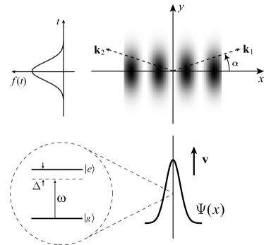
Figure 1: Scattering of the wave packet $\Psi=\Psi(x)$ of a two-level atom by a standing electromagnetic field formed by two propagating waves of wave vectors $\mathbf{k}_{1}$ and $\mathbf{k}_{2}$. The latter assume an angle $\alpha$ and $\pi-\alpha$ with respect to the $x$-axis. The field envelope along the $y$-axis translates, according to the relation $y=vt$, into the time-dependent function $f=f(t)$ as the atom propagates through the field with velocity $\mathbf{v}=v\,{\rm{\mathbf{e}}}_{y}$. The frequency $\omega$ of the field is detuned from the frequency of the atomic transition between the ground and excited states $|g\rangle$ and $|e\rangle$ by $\Delta$.

II.1 Set-up

We consider the scattering of a two-level atom off a near-resonant standing light field created by two traveling waves of wave vectors $\mathbf{k}_{1}\equiv(k\cos\alpha,k\sin\alpha)$ and $\mathbf{k}_{2}\equiv(-k\cos\alpha,k\sin\alpha)$. Both fields form an angle $\alpha$ relative to the $x$-axis of a Cartesian coordinate system as shown in Fig. 1. The two running waves have identical wave number, that is $|\mathbf{k}_{1}|=|\mathbf{k}_{2}|\equiv k$, but propagate against each other since $\left(\mathbf{k}_{1}\right)_{x}=-\left(\mathbf{k}_{2}\right)_{x}$. As a result the electric field reads

$$\mathbf{E}(t,\mathbf{r})=\mathbf{E}_{0}(\mathbf{r})\left[\sin(\mathbf{k}_{2}\mathbf{r}-\omega t)-\sin(\mathbf{k}_{1}\mathbf{r}-\omega t)\right],$$ (1)

where $\mathbf{E}_{0}=\mathbf{E}_{0}(\mathbf{r})$ describes the position-dependent real-valued amplitude of the wave with frequency $\omega$.

The time evolution of the state vector $|\Psi\rangle$ of the two-level atom interacting with the electromagnetic field $\mathbf{E}$ follows from the Schrödinger equation Sch ; Yakovlev

$$i\hbar\frac{d}{dt}|\Psi\rangle=\left(\hat{H}_{cm}+\hat{H}_{a}-\hat{\mathbf{d}}\cdot\hat{\mathbf{E}}\right)|\Psi\rangle,$$ (2)

where the Hamiltonian

$$\hat{H}_{cm}\equiv\frac{\hat{\mathbf{p}}^{2}}{2M}$$ (3)

is the kinetic energy operator of the center-of-mass motion of the atom of mass $M$. Here, $\hat{H}_{a}$ denotes the Hamiltonian of the free two-level atom with energy eigenstates $|e\rangle$ and $|g\rangle$ and the corresponding energy eigenvalues $E_{e}\equiv\hbar\omega_{e}$ and $E_{g}\equiv\hbar\omega_{g}$, shown in Fig. 1. The field frequency $\omega$ is assumed to be detuned from the frequency of the atomic transition between $|g\rangle$ and $|e\rangle$ by $\Delta\equiv\omega_{e}-\omega_{g}-\omega$. The interaction between the atom and the electromagnetic wave is described by the dipole moment operator $\hat{\mathbf{d}}$. Moreover, the carrot on $\mathbf{E}$ indicates the operator nature due to the quantum mechanical description of the motion of the atom.

The mean value of the velocity $v$ of the atom in the direction of the $y$-axis is large and remains almost constant during the scattering process. For this reason we consider this motion classically, which allows us to set $y\equiv vt$.

In contrast, the motion along the $x$-axis is described quantum mechanically. Moreover, we make the Raman-Nath approximation Sch ; Yakovlev , that is we neglect the kinetic energy operator $\hat{H}_{cm}$ in the Schrödinger equation (2). Hence, the displacement of the atom along the $x$-axis caused by the interaction with the standing light wave is assumed to be small compared to the corresponding wave length. Since $\hat{H}_{cm}$ is omitted in Eq. (2), the coordinate $x$ is considered to be a parameter. Moreover, we neglect spontaneous emission due to the small interaction time $\tau$ and the non-vanishing detuning $\Delta$.

As a result the Schrödinger equation (2) reduces to

$$i\hbar\frac{d}{dt}|\Psi\rangle\cong\left(\hat{H}_{a}-\hat{\mathbf{d}}\cdot\mathbf{E}\right)|\Psi\rangle.$$ (4)

In order to solve this equation we make the ansatz

$$|\Psi\rangle=A_{e}(t;\mathbf{r})e^{-i(\omega_{e}-\Delta/2)t}|e\rangle+A_{g}(t;\mathbf{r})e^{-i(\omega_{g}+\Delta/2)t}|g\rangle,$$ (5)

where the amplitudes $A_{g}$ and $A_{e}$ are functions of time $t$, but depend on the position vector $\mathbf{r}$ as a parameter. It is for this reason that we have dropped in Eq. (4) the carrot on $\mathbf{E}$.

Substituting the ansatz Eq. (5) into the approximate Schrödinger equation (4), we arrive at

$$i\hbar\frac{d}{dt}{{A}_{e}\choose{A}_{g}}=\hat{H}{A_{e}\choose A_{g}},$$ (6)

with the Hamiltonian

$$\hat{H}\equiv\frac{1}{2}\left(\begin{array}[]{ccc}\hbar\Delta&V^{*}\\ V&-\hbar\Delta\end{array}\right)$$ (7)

containing the complex-valued coupling matrix element

$$V(t;\mathbf{r})=-2e^{-i\omega t}\boldsymbol{\wp}\cdot\mathbf{E}(t,\mathbf{r}).$$ (8)

Here we have introduced the dipole matrix element $\boldsymbol{\wp}\equiv\langle g|\hat{\mathbf{d}}|e\rangle$, which can be considered as real-valued in the case of the two-level atom.

II.2 Matrix element of interaction

The remaining task is to derive an explicit expression for the matrix element $V$ defined by Eq. (8) in the presence of the two running waves. For this purpose we represent the sine functions in Eq. (1) as a sum of exponentials

$$\mathbf{E}=\frac{\mathbf{E}_{0}}{2i}\left[(e^{i\mathbf{k}_{2}\mathbf{r}}-e^{i\mathbf{k}_{1}\mathbf{r}})e^{-i\omega t}-(e^{-i\mathbf{k}_{2}\mathbf{r}}-e^{-i\mathbf{k}_{1}\mathbf{r}})e^{i\omega t}\right]$$ (9)

and evaluate $V$ neglecting terms oscillating with $2\omega$ which yields

$$V(t;\mathbf{r})\simeq-i\boldsymbol{\wp}\mathbf{E}_{0}(\mathbf{r})(e^{-i\mathbf{k}_{2}\mathbf{r}}-e^{-i\mathbf{k}_{1}\mathbf{r}}).$$ (10)

Next we substitute the explicit form of the wave vectors $\mathbf{k}_{1}$ and $\mathbf{k}_{2}$ into Eq. (10) and find

$$V(t;\mathbf{r})=2\boldsymbol{\wp}\mathbf{E}_{0}(x,y)e^{-iky\sin\alpha}\sin(kx\cos\alpha).$$ (11)

At this point we make use of the fact that the motion of the atom along the $y$-axis is treated classically and we can replace the $y$-coordinate by $y=vt$. Moreover, for the sake of simplicity we assume that $\mathbf{E}_{0}$ is independent of $x$, resulting in $\mathbf{E}_{0}(x,y)=\mathbf{E}_{0}(vt)=\boldsymbol{\mathcal{E}}_{0}f(t)$, where $f=f(t)$ denotes the envelope function along the $y$-axis, as indicated in Fig. 1. The coupling matrix element $V$ given by (11) takes then the form

$$V(t;\mathbf{r})=\hbar\Omega(x)f(t)e^{-i\omega_{\alpha}t}\;,$$ (12)

where

$$\omega_{\alpha}\equiv kv\sin\alpha$$ (13)

and

$$\Omega(x)\equiv\frac{2}{\hbar}\boldsymbol{\wp}\boldsymbol{\mathcal{E}}_{0}\sin(kx\cos\alpha)\equiv\Omega_{0}\sin(kx\cos\alpha)$$ (14)

are the velocity-dependent Doppler and position-dependent Rabi frequencies, respectively.

Hence, the coupling matrix element $V$ consists of the product of three terms: (i) the position-dependent coupling energy $\hbar\Omega(x)$, (ii) the envelope function $f=f(t)$, and (iii) the time-dependent phase factor $\exp(-i\omega_{\alpha}t)$ due to the motion of the atom through the field.

III Dynamical and geometric phases

In the present section we connect the Hamiltonian Eq. (7) together with the explicit expression for the matrix element $V$, Eq. (12), to the Hamiltonian used in Ref. Berry84 to derive the geometric phase. This approach allows us to take advantage of the results obtained in Ref. Berry84 . Moreover, we establish the connection between the dressed and the atomic states.

III.1 Connection to Berry’s approach

For this purpose we make the identifications

$$X\equiv{\rm Re}\,V,\;Y\equiv{\rm Im}\,V,\;Z\equiv\hbar\Delta$$ (15)

and the Hamiltonian (7) takes the form

$$H(\boldsymbol{\mathcal{R}})=\frac{1}{2}\left(\begin{array}[]{ccc}Z&X-iY\\ X+iY&-Z\end{array}\right),$$ (16)

where the real-valued parameters $X$, $Y$ and $Z$ form the cartesian coordinates of the vector $\boldsymbol{\mathcal{R}}$. Here we have chosen the calligraphic letter rather than the normal one in order to bring out the fact that the vector $\boldsymbol{\mathcal{R}}$ is not in three-dimensional position space but in parameter space.

This Hamiltonian has the eigenvalues $\varepsilon^{(\pm)}=\pm\varepsilon$ with

$$\varepsilon\equiv\frac{1}{2}\sqrt{X^{2}+Y^{2}+Z^{2}}=\frac{1}{2}\sqrt{|V|^{2}+(\hbar\Delta)^{2}}\;.$$ (17)

and the corresponding eigenstates

$$|\Psi^{(\pm)}\rangle\equiv\frac{1}{\sqrt{2\mathcal{R}(\mathcal{R}\pm Z)}}{Z\pm\mathcal{R}\choose X+iY},$$ (18)

where $\mathcal{R}=|\boldsymbol{\mathcal{R}}|$.

Now we return to the determination of the adiabaticity criterion. The condition for an adiabatic turn-on and -off of the interaction is that at any time $t$ the rate of change of the light-field amplitude is much smaller than the spacing between the time-dependent quasi-energy levels. Hence, the parameters of the system should satisfy the following inequality

$$\left|\frac{\hbar}{V}\frac{\partial V}{\partial t}\right|\ll|\varepsilon_{+}-\varepsilon_{-}|.$$ (19)

The expression Eq. (12) for the coupling matrix element $V$ allows us to cast Eq. (19) into the form

$$\left|\frac{1}{f}\frac{df}{dt}-i\omega_{\alpha}\right|\ll\sqrt{\Delta^{2}+|\Omega|^{2}f^{2}(t)}\;.$$ (20)

For a function $f(t)$ which decreases exponentially at large $t$, that is $f(t\rightarrow\pm\infty)\propto\exp(-|t|/\tau)$, we arrive at the adiabaticity criterion

$$|\Delta|\tau\gg\sqrt{1+(\omega_{\alpha}\tau)^{2}}\;.$$ (21)

In the adiabatic limit, we remain in the adiabatic states $|\Psi^{(\pm)}\rangle$ which accumulate the phases in the course of time. When the time dependence of $\boldsymbol{\mathcal{R}}$ is such that $\boldsymbol{\mathcal{R}}(t)$ returns at time $t=T$ to its initial value $\boldsymbol{\mathcal{R}}(-T)$, the two instantaneous eigenstates $|\Psi^{(\pm)}\rangle$ acquire Berry84 the dynamical and geometric phases

$$\varphi_{D}=\frac{1}{\hbar}\int\limits_{-T}^{T}\varepsilon(t)dt$$ (22)

and

$$\varphi_{B}=\iint\limits_{S_{0}}\frac{\boldsymbol{\mathcal{R}}\cdot d\mathbf{S}}{2\mathcal{R}^{3}}\;,$$ (23)

where $S_{0}$ denotes the surface of integration, i.e. the surface determined by a closed circuit forming during the one cycle of parameter change from $t=-T$ to $t=T$. As a result the eigenstates after a cyclic change read

$$|\Psi^{(\pm)}(T)\rangle=\exp(\mp i\varphi_{D})\exp(\mp i\varphi_{B})|\Psi^{(\pm)}(-T)\rangle.$$ (24)

The geometric phase is solely determined by the flux of the effective field $\boldsymbol{\mathcal{R}}/2\mathcal{R}^{3}$ through the area enclosed by the parameter $\boldsymbol{\mathcal{R}}=\boldsymbol{\mathcal{R}}(t)$ during one period of the parameter change, i.e. during the time interval $2T$.

III.2 Connection between dressed and atomic states

The dynamical as well as the geometric phase are formulated in terms of the dressed states Eq. (18) which arise due to the atom-field interaction. However, in order to observe the geometric phase in an experiment, the atom should be prepared in a well-defined free-atom internal state. For this reason we need to connect the dressed states $|\Psi^{(\pm)}\rangle$ with the atomic ones, that is with $|g\rangle$ and $|e\rangle$.

Before the atom enters the light field, that is at the time $t=-T$, the interaction $V$ vanishes, leading to $X=Y=0$ and $\mathcal{R}=|Z|=\hbar|\Delta|$. Here we have assumed for the sake of simplicity that the envelope function is a mesa function with a sharp turn-on at $-T$ and a sharp turn-off at $T$. Needless to say this assumption is not necessary and we will consider later a smooth envelope function. Due to appearance of the absolute value $|\Delta|$ of the detuning it is useful to consider the two cases of $\Delta<0$ and $\Delta>0$. Indeed, for $\Delta<0$ we find

$$|\Psi^{(+)}(-T)\rangle=|g\rangle\;\text{and}\;|\Psi^{(-)}(-T)\rangle=-|e\rangle,$$ (25)

whereas for $\Delta>0$ we arrive at

$$|\Psi^{(+)}(-T)\rangle=|e\rangle\;\text{and}\;|\Psi^{(-)}(-T)\rangle=|g\rangle.$$ (26)

Hence, in the case of $\Delta<0$ the ground and excited states follow $|\Psi^{(+)}\rangle$ and $|\Psi^{(-)}\rangle$, respectively, whereas, for $\Delta>0$ the ground and excited states follow $|\Psi^{(-)}\rangle$ and $|\Psi^{(+)}\rangle$.

By using Eqs. (5), (24), (25), and (26), we obtain the total phase

$$\varphi_{g}\equiv\beta\,{\rm sign}\Delta+\gamma,$$ (27)

of the ground state acquired during the interaction time $2T$, where

$$\beta\equiv\varphi_{D}-|\Delta|T$$ (28)

and

$$\gamma\equiv\varphi_{B}\,{\rm sign}\Delta$$ (29)

are the total dynamical and Berry phases, respectively.

The same procedure results in the total phase of the excited state

$$\varphi_{e}=-\varphi_{g}-\pi\,\Theta(-\Delta),$$ (30)

with $\Theta$ being the Heaviside function.

Note, that we have neglected the phase contributions proportional to $\omega_{g}$ and $\omega_{e}$ arising from Eq. (5), since they are independent of the coordinate of the atom. Indeed, we shall show that the Berry phase as well as the dynamical phase depend appropriately on the position and therefore can be detected by a narrowing of the atomic wave packet.

IV Circuit in parameter space

In Sec. II we have derived the explicit expression Eq. (12) for the interaction matrix element $V$ of the atom-field coupling. We are now in the position to discuss the path $\boldsymbol{\mathcal{R}}=\boldsymbol{\mathcal{R}}(t)$ in parameter space traversed in the course of time.

Since according to Eq. (15) the $Z$-component of $\boldsymbol{\mathcal{R}}$ is given by the constant detuning $\Delta$, the circuit lies parallel to the $XY$-plane and is given by

$$X(t;x)=\hbar|\Omega(x)|f(t)\cos(\omega_{\alpha}t)$$ (31)

and

$$Y(t;x)=-\hbar|\Omega(x)|f(t)\sin(\omega_{\alpha}t).$$ (32)

Due to the position-dependence of $\Omega$ the circuit depends on $x$ as a parameter.

This curve is most conveniently described by the polar coordinates

$$\rho\equiv\hbar|\Omega|f(t),\;\;\;\phi\equiv\omega_{\alpha}t$$ (33)

leading to

$$\rho=\rho(\phi)=\hbar|\Omega|f(\phi/\omega_{\alpha}).$$ (34)

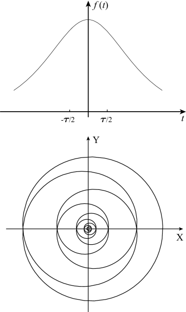
Figure 2: Translation of the electromagnetic field envelope $f=f(t)$ shown on the top into a circuit in parameter space, depicted at the bottom, illustrated here for the Eckart envelope Eq. (35). This function leads to an infinite amount of windings around the origin of parameter space.

A model of relevant for an experiment relies on a smooth envelope, for instance, by the Eckart envelope

$$f_{E}(t)\equiv\frac{1}{\cosh(t/\tau)}.$$ (35)

Although laser beams are usually modeled by a Gaussian profile, results obtained with the Eckart envelope are believed to be similar to those with a Gaussian one. Moreover, in the case of the Eckart envelope the Schrödinger equation (6) for the probability amplitudes to be in the ground and the excited state has an exact solution, which can be used to compare the results obtained within the Berry approach.

We emphasize that in the case of the Eckert envelope the amplitude $\rho$ given by Eq. (33) vanishes for $t=\pm\infty$ and consequently the circuit starts from and terminates at the origin. In the course of time the amplitude $\rho$ first increases and then decreases again. At the same time the angle $\phi$ increases monotonously. As a result the curve $\boldsymbol{\mathcal{R}}=\boldsymbol{\mathcal{R}}(t)$ defining the circuit circumvents the origin infinitely many times before it returns to it, as shown in Fig. 2. However, due to the increase and decrease of $\rho$ not all windings will be visible. The number of the prominent loops is determined by the value of $\omega_{\alpha}\tau$.

V Explicit expressions for phases

In the preceding section we have discussed the form of the circuit in parameter space dictated by the longitudinal mode function of the electromagnetic field. In the present section we calculate the resulting geometric and dynamical phases and analyze the weak-field limit.

V.1 General case

We start by obtaining explicit formulae for the phases due to an arbitrary but smooth envelope function. In Appendix A we rederive these expressions within the WKB-approach.

V.1.1 Geometric phase

According to Eq. (23) we have to calculate the flux of the effective field $\boldsymbol{\mathcal{R}}/(2\mathcal{R}^{3})$ through the area enclosed by the circuit in parameter space. Since the vector normal to this surface is in the opposite direction to the $Z$-axis of the Cartesian coordinate system we find that $\boldsymbol{\mathcal{R}}\cdot d\mathbf{S}=-\hbar\Delta dS$ and Eq. (23) with the definition Eq. (29) reduces to

$$\gamma=-\frac{1}{2}\hbar|\Delta|\int dX\int dY\frac{1}{(X^{2}+Y^{2}+(\hbar\Delta)^{2})^{3/2}}\;.$$ (36)

In terms of the polar coordinates $\rho$ and $\phi$ defined by Eq. (33) this integral takes the form

$$\gamma=-\frac{1}{2}\hbar|\Delta|\int\limits_{\phi_{i}}^{\phi_{f}}d\phi\int\limits_{0}^{\rho(\phi)}\frac{\rho\,d\rho}{(\rho^{2}+\hbar^{2}\Delta^{2})^{3/2}}\;.$$ (37)

Here the upper limit $\rho=\rho(\phi)$ of the radial integral depends on the circuit in parameter space parameterized by the angle $\phi$. The integration over $\phi$ runs between the initial $\phi_{i}\equiv\phi(-T)$ and final $\phi_{f}\equiv\phi(T)$ angles of the curve. Their precise form is dictated by the shape of the circuit.

The integration over $\rho$ can be performed and with the help of Eq. (34) and the new integration variable $t\equiv\phi/\omega_{\alpha}$ we arrive at

$$\gamma=\frac{\omega_{\alpha}}{2}\int\limits_{-T}^{T}dt\left(\frac{|\Delta|}{\sqrt{|\Delta|^{2}+|\Omega(x)|^{2}f^{2}(t)}}-1\right),$$ (38)

or

$$\gamma=\frac{\omega_{\alpha}}{2}\int\limits_{-T}^{T}dt\left(\frac{1}{\sqrt{1+a^{2}(x)f^{2}(t)}}-1\right),$$ (39)

where

$$a(x)\equiv\frac{|\Omega(x)|}{|\Delta|}$$ (40)

is the dimensionless Rabi frequency. The position dependence of the geometric phase arises from the position dependence of $a=a(x)$.

V.1.2 Dynamical phase

Next we turn to the dynamical phase. For this purpose we substitute the expression for $V$, Eq. (12), into the one for the quasi-energy $\varepsilon$, Eq. (17), and find

$$\varepsilon(t)=\frac{\hbar}{2}\sqrt{\Delta^{2}+|\Omega(x)|^{2}f^{2}(t)}.$$ (41)

Together with Eqs. (22) and (28) for the total dynamical phase, we arrive at

$$\beta=\frac{1}{2}\int\limits_{-T}^{T}dt\left(\sqrt{|\Delta|^{2}+|\Omega(x)|^{2}f^{2}(t)}-|\Delta|\right),$$ (42)

or

$$\beta=\frac{|\Delta|}{2}\int\limits_{-T}^{T}dt\left(\sqrt{1+a^{2}f^{2}(t)}-1\right),$$ (43)

where we have recalled the definition Eq. (40) of the dimensionless Rabi frequency $a$.

When we compare the expressions Eqs. (38) and (42) for the geometric and the dynamical phases we find the identity

$$\gamma=\omega_{\alpha}\frac{\partial\beta}{\partial|\Delta|}\,,$$ (44)

which is reminiscent of the Kramers-Kronig relations. However, the WKB-analysis presented in Appendix A shows that Eq. (44) is merely a consequence of a Taylor expansion in powers of $\omega_{\alpha}/|\Delta|$. It is interesting to note that in the formalism employed in the preceding sections this fact is hidden.

V.2 Weak-field limit

Finally we consider these phases in the weak-field limit, that is for $a\ll 1$, when Eq. (43) for the dynamical phase reduces to

$$\beta\cong\frac{1}{4}\,|\Delta|a^{2}\int\limits_{-T}^{T}dtf^{2}(t),$$ (45)

while the geometric phase given by Eq. (39) reads

$$\gamma\cong-\frac{1}{4}\,\omega_{\alpha}a^{2}\int\limits_{-T}^{T}dtf^{2}(t).$$ (46)

In Appendix A we rederive these expressions directly by second-order perturbation theory.

A comparison between Eqs. (45) and (46) reveals that in the weak-field limit, $|\Omega|\ll|\Delta|$, the ratio of the geometric and dynamical phases is equal to

$$\left|\frac{\gamma}{\beta}\right|=\frac{\omega_{\alpha}}{|\Delta|},$$ (47)

and thus independent of the field envelope.

We conclude by estimating this ratio for typical experimental values. For instance, for the $\quad 1s_{5}(J=2)\rightarrow 2p_{3}(J=3)$ transition in argon Oberthaler , the wave length $\lambda=812\,\text{nm}$, the resonance detuning $\Delta\cong 3\cdot 10^{7}\,\text{s}^{-1}$, the velocity $v_{y}=700\,\text{m/s}$ and angle $\alpha=10^{-3}$, we obtain $|\gamma/\beta|\cong 0.1$, which is feasible in an experiment.

VI Application to Eckart envelope

In this section we evaluate the geometric and dynamical phases for the Eckart envelope defined by Eq. (35). For the details of the integrations we refer to Appendix B and C.

VI.1 Geometric phase

For the Eckart envelope we have $T=\infty$ and Eq. (39) takes the form

$$\gamma_{E}=\omega_{\alpha}\tau\int\limits_{0}^{\infty}d\theta\left(\frac{\cosh\theta}{\sqrt{\cosh^{2}\theta+a^{2}}}-1\right),$$ (48)

where we have introduced $\theta\equiv t/\tau$ and used the symmetry of the integrand.

In Appendix B we perform this integral and find the geometric phase

$$\gamma_{E}(x)=-\frac{1}{2}\,\omega_{\alpha}\tau\ln\left(1+a^{2}(x)\right),$$ (49)

which in the weak-field limit $a(x)\ll 1$ reduces to

$$\gamma_{E}(x)\cong-\frac{1}{2}\,\omega_{\alpha}\tau a^{2}(x).$$ (50)

We conclude by noting that we can rederive the expression Eq. (49) for $\gamma_{E}$ by decomposing the path in the parameter space into a sequence of closed circuits and calculating the sum of the fluxes through each of these areas, as shown in Appendix C.

VI.2 Dynamical phase

For the Eckart envelope the expression Eq. (43) for the dynamical phase takes the form

$$\beta_{E}=|\Delta|\tau\int\limits_{0}^{\infty}d\theta\left(\sqrt{1+\frac{a^{2}}{\cosh^{2}\theta}}-1\right)$$ (51)

and according to Appendix B we find

$$\beta_{E}=|\Delta|\tau\left[a\arctan(a)-\frac{1}{2}\ln(1+a^{2})\right],$$ (52)

which for $a^{2}\ll 1$ reduces to

$$\beta_{E}\cong\frac{1}{2}|\Delta|\tau a^{2}=\frac{|\Delta|}{\omega_{\alpha}}\,|\gamma_{E}|.$$ (53)

In the last step we have recalled Eq. (50) for $\gamma_{E}$.

Hence, we confirm the fact that the ratio of the geometric to the dynamical phase is given by Eq. (47).

VII Cancellation of dynamical phase

Next we use the results obtained in the previous sections to propose a scheme to cancel the dynamical phase, which always dominates the geometric one. Moreover, due to its dependence on the energy of the system, the dynamical phase is particularly sensitive to the slightest change of the parameters.

From the expressions Eqs. (27) and (30) for the total phases acquired by the ground and excited states, we recall that the dynamical part given by $\beta\,{\rm sign}(\Delta)$ depends on the sign of the detuning $\Delta$, whereas the geometric part $\gamma$ only on its absolute value.

This fact allows us to suggest a rather intuitive scheme to compensate the dynamical phase. We propose to use two consecutive interactions of the atom with the standing waves, that is, firstly with blue-detuned waves ($\Delta>0$), secondly with red-detuned waves ($\Delta^{\prime}\equiv-\Delta<0$). Here we have introduced a prime to indicate the second standing wave. As a result of the opposite signs of the detunings, the dynamical contributions cancel each other provided the condition $k\cos\alpha=k^{\prime}\cos\alpha^{\prime}$ is fulfilled, or when the position-dependent Rabi frequencies $\Omega(x)$ and $\Omega^{\prime}(x)$ defined by Eq. (14) are equal.

At the same time, the geometric phases add up and result in the total phase

$$\varphi_{g}^{(tot)}=\varphi_{g}+\varphi_{g}^{\prime}=\gamma+\gamma^{\prime}$$ (54)

of the ground state.

Thus, in a scheme of two consecutive scatterings of the atom by oppositely detuned standing waves, we obtain a cancellation of the dynamical phase and summation of the Berry phase. Of course, the time interval between the two interaction zones should be larger than the interaction time $\tau$ itself, in order to be consistent with the adiabatic approximation on the turn-on and turn-off of the interactions.

VIII Focusing due to geometric phase

In the previous section we have shown that in our scattering setup with first an interaction with the red-detuned wave, and then with the blue-detuned wave, the atom acquires only the geometric phase. We now demonstrate that this phase manifests itself in a focusing of the atomic wave packet.

For this purpose we assume for the wave function of the center-of-mass motion of an atom in the ground state moving in the $y$-direction a Gaussian

$$\Psi_{0}(x)\equiv\frac{1}{(\sqrt{\pi}\Delta x_{0})^{1/2}}\exp\left[-\frac{x^{2}}{2\Delta x_{0}^{2}}+i\gamma(x)\right]$$ (55)

of width $\Delta x_{0}$ and the additional scattering-induced geometric phase $\gamma(x)$.

The time evolution of this wave packet in the absence of an external field is given by

$$\Psi(x,t)=\sqrt{\frac{M}{2\pi i\hbar t}}\int\limits_{-\infty}^{\infty}dx^{\prime}\exp\left[i\frac{M}{2\hbar\,t}(x-x^{\prime})^{2}\right]\Psi_{0}(x^{\prime}).$$ (56)

In the case of the Eckart envelope and in the limit of $k\Delta x_{0}<1$ and $(|\Omega_{0}|/|\Delta|)(k\Delta x_{0})<1$, the geometric phase $\gamma(x)$ given by Eq. (49) near the nodes of the standing wave, for instance near $x=0$, is a quadratic function

$$\gamma(x)\cong-\frac{b}{2}\frac{x^{2}}{\Delta x_{0}^{2}}$$ (57)

of $x$ with

$$b\equiv\omega_{\alpha}\tau\,\frac{|\Omega_{0}|^{2}}{|\Delta|^{2}}(k\cos\alpha\Delta x_{0})^{2}.$$ (58)

Here we have used the definitions Eqs. (14) and (40).

By substituting the initial wave function Eq. (55) into Eq. (56), we obtain the time-dependent distribution

$$\left|\Psi(x,t)\right|^{2}=\frac{1}{\sqrt{\pi}\Delta x(t)}\exp\left(-\frac{x^{2}}{\Delta x^{2}(t)}\right)$$ (59)

of finding an atom with the coordinate $x$, where the width

$$\Delta x(t)\equiv\Delta x_{0}\sqrt{\left(1-b\frac{t}{t_{s}}\right)^{2}+\left(\frac{t}{t_{s}}\right)^{2}}.$$ (60)

is determined by the initial width $\Delta x_{0}$ and the Berry phase contribution. Here $t_{s}\equiv M\Delta x_{0}^{2}/\hbar$ is the characteristic time of field-free spreading, that is

$$\Delta x^{(0)}(t)\equiv\Delta x_{0}\sqrt{1+\frac{t^{2}}{t_{s}^{2}}}\,.$$ (61)

The minimal possible width

$$\Delta x_{min}\equiv\frac{\Delta x_{0}}{\sqrt{1+b^{2}}}$$ (62)

of the packet is reached at the time

$$t_{min}=\frac{b}{1+b^{2}}\,t_{s}.$$ (63)

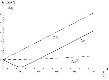
Figure 3: Influence of the geometric phase on the free propagation of an atomic wave packet represented by its time-dependent width $\Delta x(t)$ given by Eq. (60). For an atom in the ground state ($\Delta x_{g}$ and $b=5$) the wave packet first focuses and then spreads, whereas for the excited state ($\Delta x_{e}$ and $b=-5$) it spreads from the beginning. This spreading is larger than that associated with the free propagation of the Gaussian ($\Delta x^{(0)}$ and $b=0$) given by Eq. (61).

In Fig. 3, we present the focusing of the atomic wave packet induced by the geometric phase for relatively small values of the parameter $b$. For example, the value $b\approx 5$ is achieved for $\omega_{\alpha}\tau=4\pi$, the Rabi frequency $\Omega_{0}=1.8\,|\Delta|$ and the initial width $k\Delta x_{0}=0.25$. For $b=5$ the expression Eq. (62) for the minimal width predicts a shrinking up to around five times compared to the initial width, as indicated by the solid curve on Fig. 3 denoted by $\Delta x_{g}$. After the point $t\approx 0.19\,t_{s}$ the wave packet expands faster than the free wave packet represented by the dashed line $\Delta x^{(0)}$.

The atom in the excited state acquires the same geometric phase as the ground state but with the opposite sign. Therefore, the parameter $b$ determining the narrowing appears with the opposite sign and results in an accelerated spreading rather than a focusing of the wave packet, as shown by $\Delta x_{e}$ in Fig. 3.

IX Conclusions

In this article we propose a scheme to observe the geometric phase in atom optics based on the scattering of a two-level atom by two consecutive standing light waves with the same envelope but opposite detunings. The dynamical and the geometric phases acquired by the two-level atom during the interaction are calculated within (i) the rotating wave approximation, (ii) the Raman-Nath approximation, and (iii) adiabatically slow switch-on and -off of the interaction. Both the dynamical and the geometric phases are evaluated for a field envelope given by the Eckart function.

We now specify the conditions under which these approximations are valid and self-consistent. Indeed, the velocity acquired due to a resonant atom-field interaction can be estimated as

$$\langle v_{x}\rangle\sim\frac{\hbar k}{M}\,\Omega_{0}\tau,$$

where $\Omega_{0}$ is a characteristic value of the Rabi frequency. Hence, we can omit the kinetic energy operator in the Schrödinger equation when $\langle v_{x}\rangle\tau\ll 1/k$, or

$$\omega_{rec}\tau^{2}\Omega_{0}\ll 1,$$

with $\omega_{rec}\equiv\hbar k^{2}/(2M)$ being the recoil frequency.

Moreover, we can neglect the spontaneous emission due to the small interaction time $\tau$, provided

$$\Gamma\tau w\lesssim 1,$$

where $\Gamma$ and $w$ are the spontaneous emission rate and the occupation probability of the excited level, respectively. In the case of near resonance, $|\Delta|>\Omega_{0}$, the maximum value of the population probability is $w\sim(\Omega_{0}/\Delta)^{2}$.

In a sequence of two such scattering arrangements with opposite signs of their detunings the dynamical phases compensate each other, whereas the geometric phases add. Therefore, the final state of the atom is different from the initial one only by the acquired Berry phase, which in our case depends not only on the internal, but also on the external degrees of freedom, such as the position of atom. This dynamical phase cancellation provides us with a completely different technique of measuring the geometric phase, employing the narrowing of the atomic wave-packet prepared initially in the ground state. This novel suggestion of the Berry phase measurement based on self-lensing beneficially differs from the previous interferometric schemes of observing the geometric phase and might also constitute a useful tool in atomic lithography.

The familiar WKB-technique is used as an independent method to verify the results obtained within the standard approach Berry84 and the results are shown to coincide. However, we emphasize that the treatment of Ref. Berry84 is more general in the sense that it can be employed for any dependence of the interaction envelope and the detuning on time. We consider in this paper the particular case of a constant detuning.

We conclude by emphasizing again that the Raman-Nath regime takes place for a small interaction time $\tau$, that is $\tau\ll 1/(\omega_{rec}\Omega_{0})^{1/2}$. In this case, we are allowed to neglect the kinetic energy operator. However, for large interaction times, that is for $1/(\omega_{rec}\Omega_{0})^{1/2}\ll\tau\ll 1/\Gamma$ it should be taken into account. To do this in an exact way we could consider the scattering of the atom by a sequence of two near-resonant running rather than standing light waves PM . In this case the formulae for the geometric and dynamical phases are analogous to those of the standing wave case, but independent on the external atomic degrees of freedom, i.e. the atomic position. Therefore, no lensing occurs and we can only use the standard interferometric scheme for the observation of the geometric phase.

Appendix A Alternative derivation of phases

In this appendix we present alternative routes toward the expressions Eqs. (39) and (43) obtained within Berry’s formalism. To solve the Schrödinger equation (4) we make the ansatz

$$|\Psi\rangle=\tilde{A}_{e}(t;{\bf r})\,e^{-i(\omega_{e}-\tilde{\Delta}/2)t}|e\rangle+\tilde{A}_{g}(t;{\bf r})\,e^{-i(\omega_{g}+\tilde{\Delta}/2)t}|g\rangle,$$ (64)

which is different from Eq. (5) due to the effective detuning

$$\tilde{\Delta}\equiv\Delta+\omega_{\alpha}.$$ (65)

Substituting Eq. (64) into Eq. (4) and making the rotating wave approximation, we arrive at

$$i\hbar\frac{d}{dt}\left({\tilde{A}_{e}\atop\tilde{A}_{g}}\right)=\frac{1}{2}\begin{pmatrix}\hbar\tilde{\Delta}&\tilde{V}\\ \tilde{V}&-\hbar\tilde{\Delta}\end{pmatrix}\left({\tilde{A}_{e}\atop\tilde{A}_{g}}\right),$$ (66)

where in contrast to $V$ given by Eq. (12) the coupling matrix element

$$\tilde{V}(t;\mathbf{r})=\hbar\Omega(x)f(t)\equiv\hbar\tilde{\Omega}(x,t)$$ (67)

is now real and depends on time only through the envelope $f(t)$, describing the adiabatic turn-on and turn-off of the interaction.

Two approaches to solve Eq. (66) and obtain the relevant phases offer themselves : (i) the WKB-technique and (ii) second-order perturbation theory.

A.1 WKB-approach

In order to transform the two first order differential equations, Eq. (66), into a single one of second order, we introduce the two functions

$$\left({u}\atop{v}\right)\equiv\frac{1}{2}\left({\tilde{A}_{g}+\tilde{A}_{e}}\atop{\tilde{A}_{e}-\tilde{A}_{g}}\right),$$ (68)

resulting in the differential equation Fedorov

$$\frac{d^{2}}{dt^{2}}u+\frac{1}{4}\left(\tilde{\Delta}^{2}+\tilde{\Omega}^{2}+2i\frac{d\tilde{\Omega}}{dt}\right)u=0$$ (69)

for $u=u(t)$.

This equation can be represented in a form similar to the stationary Schrödinger equation in position space by introducing the dimensionless variable $\xi\equiv t/\tau$, where $\tau$ is the characteristic time scale of the envelope $f$. In terms of $\xi$, Eq. (69) reads

$$\frac{1}{\tau^{2}}\frac{d^{2}}{d\xi^{2}}\;u+\left(\tilde{\varepsilon}^{2}+\frac{i}{2\tau}\frac{d\tilde{\Omega}}{d\xi}\right)u=0,$$ (70)

where

$$\tilde{\varepsilon}(\xi)\equiv\frac{1}{2}\sqrt{\tilde{\Delta}^{2}+\tilde{\Omega}^{2}(\xi)}\;.$$ (71)

Equation (70) is analogous to the stationary one-dimensional Schrödinger equation where $\xi$ and $\tilde{\varepsilon}$ play the role of the ”effective coordinate” and ”effective momentum”, respectively. The small parameter $1/\tau$ mimics Planck’s constant in the conventional WKB-approach.

Due to the adiabaticity condition

$$\frac{1}{\tau\tilde{\varepsilon}^{2}}\cfrac{d\tilde{\varepsilon}}{d\xi}\ll 1,$$ (72)

we can employ the semiclassical approach to search for the solution $u(\xi)$ in the form

$$u(\xi)=e^{i\tau S(\xi)},$$ (73)

where the complex-valued function $S(\xi)$ obeys the equation

$$-\left(\frac{dS}{d\xi}\right)^{2}+\tilde{\varepsilon}^{2}+\frac{i}{\tau}\frac{d^{2}S}{d\xi^{2}}+\frac{i}{2\tau}\frac{d\tilde{\Omega}}{d\xi}=0\,.$$ (74)

Within the WKB approach $S(\xi)$ is expanded into the perturbation series

$$S(\xi)=S^{(0)}(\xi)+\frac{1}{\tau}S^{(1)}(\xi)+\frac{1}{\tau^{2}}S^{(2)}(\xi)+\,...$$ (75)

in powers of $1/\tau$ and from Eq. (74) we find the zero-order term

$$S^{(0)}(\xi)=\pm\int\limits_{-T/\tau}^{\xi}d\xi^{\prime}\;\tilde{\varepsilon}(\xi^{\prime})$$ (76)

and the first adiabatic correction

$$S^{(1)}(\xi)=\frac{i}{2}\left[\ln\left(\frac{2\tilde{\varepsilon}(\xi)}{|\tilde{\Delta}|}\right)\pm\ln{\mathcal{N}}(\xi)\right]$$ (77)

with

$${\mathcal{N}}(\xi)\equiv\frac{\tilde{\Omega}(\xi)}{|\tilde{\Delta}|}+\left(1+\frac{\tilde{\Omega}^{2}(\xi)}{\tilde{\Delta}^{2}}\right)^{1/2}.$$ (78)

The second term on the right-hand side of Eq. (77) is a consequence of the last term in the left-hand side of Eq. (74) and appears in addition to the conventional WKB solution. Moreover, the next-order correction to $S$ gives negligible contribution to $u$.

The general solution of Eq. (70) can then be written in the form

$$u(\xi)=\sqrt{\frac{|\tilde{\Delta}|}{2\tilde{\varepsilon}}}\sum_{\pm}A_{\pm}\exp\left[\pm i\tau\int\limits_{-T/\tau}^{\xi}d\xi^{\prime}\tilde{\varepsilon}(\xi^{\prime})\mp\frac{\ln{\mathcal{N}(\xi)}}{2}\right],$$ (79)

where the coefficients $A_{\pm}$ can be found from the initial conditions $\tilde{A}_{g}(-T)=1$ and $\tilde{A}_{e}(-T)=0$ for $\tilde{A}_{g}(t)$ and $\tilde{A}_{e}(t)$. By using Eq. (68) and the connection between $u$ and $v$ we get $u(\xi)=1/2$ and $(du/d\xi)=i\tilde{\Delta}\tau/4$ at $\xi=-T/\tau$, which results in

$$A_{\pm}=\frac{1}{4}(1\pm{\rm sign}\tilde{\Delta})=\frac{1}{2}\,\Theta(\pm\tilde{\Delta}).$$ (80)

Here we have used the fact that at $\xi=-T/\tau$ the Rabi frequency $\tilde{\Omega}$ defined by Eq. (67) vanishes and therefore ${\mathcal{N}}(-T/\tau)=1$ and $2\tilde{\varepsilon}(-T/\tau)=|\tilde{\Delta}|$.

The same procedure can be applied to find $v(t)$, leading to $v(t)=-u(t)$. We then obtain the relations $\tilde{A}_{g}=u-v=2u$ and $\tilde{A}_{e}=u+v=0$. The latter confirms the fact that there are no transitions into the excited state due to the adiabatically slow time dependence of the interaction.

Thus, the probability amplitude $\tilde{A}_{g}$ is given by

$$\tilde{A}_{g}(t)=\sqrt{\frac{|\tilde{\Delta}|}{2\tilde{\varepsilon}}}\sum_{\pm}\Theta(\pm\tilde{\Delta})\exp\left[\pm i\tau\int\limits_{-T}^{t}dt^{\prime}\tilde{\varepsilon}(t^{\prime})\mp\frac{\ln{\mathcal{N}}}{2}\right].$$ (81)

By taking into account the exponential prefactor $\exp(-i\tilde{\Delta}t/2)$ in Eq. (64), we obtain from Eq. (81) the total phase

$$\tilde{\varphi}_{g}=\frac{{\rm sign}(\tilde{\Delta})}{2}\int\limits_{-T}^{T}dt\left(\sqrt{\tilde{\Delta}^{2}+\tilde{\Omega}^{2}(t)}-|\tilde{\Delta}|\right)$$ (82)

acquired by the ground state at $t=T$, when the interaction switches off, that is $\tilde{A}_{g}(T)\equiv\exp(i\tilde{\varphi}_{g})$.

According to Eq. (82) the total phase $\tilde{\varphi}_{g}$ is a function of the effective detuning $\tilde{\Delta}=\Delta+\omega_{\alpha}$. When $\omega_{\alpha}\ll|\Delta|$ we can expand $\tilde{\varphi}_{g}$ into a Taylor series

$$\tilde{\varphi}_{g}(\tilde{\Delta})=\tilde{\varphi}_{g}(\Delta+\omega_{\alpha})\cong\tilde{\varphi}_{g}(\Delta)+\omega_{\alpha}\frac{\partial\tilde{\varphi}_{g}}{\partial\Delta}$$ (83)

over $\omega_{\alpha}/|\Delta|$ and arrive at

$$\tilde{\varphi}_{g}=\frac{\Delta}{2}\int\limits_{-T}^{T}dt\left(\sqrt{1+a^{2}f^{2}(t)}-1\right)$$

$$+\frac{\omega_{\alpha}}{2}\int\limits_{-T}^{T}dt\left(\frac{1}{\sqrt{1+a^{2}f^{2}(t)}}-1\right).$$ (84)

Here we have recalled the definitions Eqs. (40) and (67).

A comparison between Eqs. (27) and (84) reveals that the first term in Eq. (84) gives the expression Eq. (43) for the dynamical phase, whereas the second term is the geometric phase given by Eq. (39). Moreover, Eq. (83) shows that the Kramers-Kronig-like relation, Eq. (44), between the dynamical and geometric phases is a consequaence of a Taylor expension.

We conclude by noting that Eq. (69) for the Eckart envelope can be solved exactly Fedorov in terms of hypergeometric functions. In the adiabatic limit, $|\Delta|\tau\gg 1$ and $\omega_{\alpha}\ll|\Delta|$, the probability amplitudes $\tilde{A}_{g}$ and $\tilde{A}_{e}$ obtained from the exact solution coincide PM with those derived within the WKB approach.

A.2 Perturbation theory

The Schrödinger equation (66) can be solved perturbatively using the coupling matrix element $\tilde{V}$ as the expansion parameter. Indeed, the second-order correction to the probability amplitudes $\tilde{a}_{e}\equiv\tilde{A}_{e}\,e^{i\tilde{\Delta}t/2}$ and $\tilde{a}_{g}\equiv\tilde{A}_{g}\,e^{-i\tilde{\Delta}t/2}$ are given by

$$\tilde{a}_{e}^{(2)}(T)=-\frac{\tilde{a}_{e}(-T)}{4}\int\limits_{-T}^{T}dt\tilde{V}(t)e^{i\tilde{\Delta}t}\int\limits_{-T}^{t}dt^{\prime}\tilde{V}(t^{\prime})e^{-i\tilde{\Delta}t^{\prime}}$$ (85)

and

$$\tilde{a}_{g}^{(2)}(T)=-\frac{\tilde{a}_{g}(-T)}{4}\int\limits_{-T}^{T}dt\tilde{V}(t)e^{-i\tilde{\Delta}t}\int\limits_{-T}^{t}dt^{\prime}\tilde{V}(t^{\prime})e^{i\tilde{\Delta}t^{\prime}}.$$ (86)

By using the adiabaticity condition Eq. (19), we find

$$\int\limits_{-T}^{t}dt^{\prime}\tilde{V}(t^{\prime})e^{\pm i\tilde{\Delta}t^{\prime}}\cong\mp\,\frac{i\tilde{V}(t)}{\tilde{\Delta}}\,e^{\pm i\tilde{\Delta}t}\,,$$

which results in

$$\tilde{a}_{e}(T)=\tilde{a}_{e}(-T)+\tilde{a}_{e}^{(2)}=\tilde{a}_{e}(-T)\left[1-\frac{i}{4}\int\limits_{-T}^{T}dt\frac{\tilde{V}^{2}(t)}{\tilde{\Delta}}\right],$$

that is

$$\tilde{a}_{e}(T)\cong\tilde{a}_{e}(-T)e^{-i\varphi}$$ (87)

with the phase

$$\varphi\equiv\frac{1}{4}\int\limits_{-T}^{T}dt\frac{\tilde{V}^{2}(t)}{\tilde{\Delta}}.$$ (88)

Similarly, we obtain

$$\tilde{a}_{g}(T)=\tilde{a}_{g}(-T)+\tilde{a}_{g}^{(2)}=\tilde{a}_{g}(-T)\left[1+\frac{i}{4}\int\limits_{-T}^{T}dt\frac{\tilde{V}^{2}(t)}{\tilde{\Delta}}\right],$$

or

$$\tilde{a}_{g}(T)\cong\tilde{a}_{g}(-T)e^{i\varphi}.$$ (89)

By using the definitions Eqs. (40), (65) and (67) we derive for the total phase $\varphi$ given by Eq. (88) the expression

$$\varphi=\frac{a^{2}}{4}\frac{\Delta^{2}}{\Delta+\omega_{\alpha}}\int\limits_{-T}^{T}dtf^{2}(t).$$ (90)

In the case when $\omega_{\alpha}\ll|\Delta|$ the phase reads

$$\varphi\cong\frac{a^{2}}{4}\Delta\int\limits_{-T}^{T}dtf^{2}(t)-\frac{a^{2}}{4}\omega_{\alpha}\int\limits_{-T}^{T}dtf^{2}(t).$$ (91)

With the help of Eq. (27) we find that the first and second terms in Eq. (91) give the dynamical and geometric phases in the weak-field limit defined by Eqs. (45) and (46), respectively.

Appendix B Evaluation of integrals

In this appendix we evaluate the integrals Eqs. (48) and (51) determining the geometric and dynamical phase in the case of the Eckart envelope. We note that some of the relations are also useful for Appendix C.

B.1 Integral determining the geometric phase

In order to calculate the integral

$$I_{E}\equiv\int\limits_{0}^{\infty}d\theta\left[\frac{\cosh\theta}{\sqrt{\cosh^{2}\theta+a^{2}}}-1\right]$$ (92)

we recall the integral relation

$$\int d\theta\frac{\cosh\theta}{\sqrt{\cosh^{2}\theta+a^{2}}}=\ln\left(\sinh\theta+\sqrt{\cosh^{2}\theta+a^{2}}\;\right)$$ (93)

and find

$$I_{E}=\lim_{\theta\rightarrow\infty}\left\{\ln\left[\frac{\sinh\theta+\sqrt{\cosh^{2}\theta+a^{2}}}{\sqrt{1+a^{2}}}\right]-\theta\right\},$$ (94)

which with the help of the asymptotic behavior

$$\sinh\theta\cong\cosh\theta\cong\frac{1}{2}\,e^{\theta}$$ (95)

in the limit of $\theta\rightarrow\infty$ reduces to

$$I_{E}=-\frac{1}{2}\ln\left(1+a^{2}\right).$$ (96)

B.2 Integral determining the dynamical phase

The dynamical phase is determined by the integral

$$\tilde{I}_{E}\equiv\int\limits_{0}^{\infty}d\theta\left(\sqrt{1+\frac{a^{2}}{\cosh^{2}\theta}}-1\right),$$ (97)

or

$$\tilde{I}_{E}\equiv a^{2}\int\limits_{0}^{\infty}\frac{d\theta}{\cosh^{2}\theta}\frac{1}{1+\sqrt{1+a^{2}\cosh^{-2}\theta}}.$$

The change of the integration variable

$$\sin\vartheta\equiv\sqrt{\frac{a^{2}}{1+a^{2}}}\,\tanh\theta$$

gives

$$\tilde{I}_{E}=a\left[\arctan(a)-\int\limits_{0}^{\arctan(a)}\frac{d\vartheta}{1+\sqrt{1+a^{2}}\cos\vartheta}\right].$$ (98)

When we recall the integral relation

$$\int\limits_{0}^{\vartheta_{0}}\frac{d\vartheta}{A+B\cos\vartheta}=$$

$$\frac{1}{\sqrt{B^{2}-A^{2}}}\ln\Bigg{|}\frac{\sqrt{B^{2}-A^{2}}\tan(\vartheta_{0}/2)+A+B}{\sqrt{B^{2}-A^{2}}\tan(\vartheta_{0}/2)-A-B}\Bigg{|}$$

for $A<B$, we arrive at

$$\tilde{I}_{E}=a\arctan(a)-\frac{1}{2}\ln(1+a^{2}).$$ (99)

Appendix C Evaluation of flux

In this appendix we evaluate the flux through the area in parameter space defined by the trajectory following from the Eckart envelope of the electromagnetic field. In this case the separation of the trajectory from the origin, determined by the strength of the envelope, first increases from zero to a maximum value and then decreases again to zero. As a result, we obtain infinitely many windings and thus infinitely many areas of different sizes.

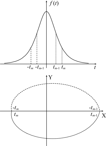
Figure 4: Translation of the field envelope $f=f(t)$ during two symmetrically located time intervals (top) into a closed circuit in parameter space (bottom). Indeed, the $m$-th circuit arises from the envelope $f=f(t)$ during the time intervals $-t_{m}\leq t\leq-t_{m-1}$ and $t_{m-1}\leq t\leq t_{m}$.

In order to calculate the total flux through them, we present the expression Eq. (37) for the geometric phase $\gamma_{E}$ as a sum

$$\gamma=-\sum_{m}\frac{1}{2}\int\limits_{\phi_{i}^{m}}^{\phi_{f}^{m}}d\phi\int\limits_{0}^{\rho(\phi)}\frac{\tilde{\rho}\,d\tilde{\rho}}{(1+\tilde{\rho}^{2})^{3/2}}\equiv\sum_{m}\gamma^{(m)}$$ (100)

of the fluxes through the $m$-th area with

$$\rho(\phi)\equiv\frac{a}{\cosh[\phi/(\omega_{\alpha}\tau)]}.$$ (101)

Here we have recalled the definitions Eqs. (34), (35) and (40).

In order to perform the integration in Eq. (100) we need to determine the angles $\phi$ corresponding to the path defining the $m$-th area. This path is dictated by the envelope during the time intervals $-t_{m}\leq t\leq-t_{m-1}$ and $t_{m-1}\leq t\leq t_{m}$, where $t_{m}\equiv m\pi/\omega_{\alpha}$, as shown in Fig. 4. Since $\phi=\omega_{\alpha}t$ these time domains translate into the integration intervals $-\phi_{m}\leq\phi\leq-\phi_{m-1}$ and $\phi_{m-1}\leq\phi\leq\phi_{m}$ with $\phi_{m}\equiv m\pi$.

Therefore, the geometric phase $\gamma^{(m)}$ given by the flux through the $m$-th area reads

$$\gamma^{(m)}=-\frac{1}{2}\int\limits_{-m\pi}^{-(m-1)\pi}d\phi\int\limits_{0}^{\rho(\phi)}\frac{\tilde{\rho}\,d\tilde{\rho}}{(1+\tilde{\rho}^{2})^{3/2}}$$

$$-\frac{1}{2}\int\limits_{(m-1)\pi}^{m\pi}d\phi\int\limits_{0}^{\rho(\phi)}\frac{\tilde{\rho}\,d\tilde{\rho}}{(1+\tilde{\rho}^{2})^{3/2}}\,,$$ (102)

which due to the symmetry of the Eckart envelope giving rise via Eq. (101) to $\rho(-\phi)=\rho(\phi)$ simplifies to

$$\gamma^{(m)}=-\int\limits_{(m-1)\pi}^{m\pi}d\phi\int\limits_{0}^{\rho(\phi)}\frac{\tilde{\rho}\,d\tilde{\rho}}{(1+\tilde{\rho}^{2})^{3/2}}\,,$$ (103)

or

$$\gamma^{(m)}=\omega_{\alpha}\tau\int\limits_{\theta_{m-1}}^{\theta_{m}}d\theta\left(\frac{\cosh\theta}{\sqrt{\cosh^{2}\theta+a^{2}}}-1\right)$$ (104)

with $\theta_{m}\equiv m\pi/(\omega_{\alpha}\tau)$.

With the help of the integral relation Eq. (93) we arrive at

$$\gamma^{(m)}=\omega_{\alpha}\tau\left(\ln\frac{F_{m}}{F_{m-1}}-\frac{\pi}{\omega_{\alpha}\tau}\right),$$ (105)

where

$$F_{m}\equiv\sinh\theta_{m}+\sqrt{\cosh^{2}\theta_{m}+a^{2}}.$$

The total geometric phase $\gamma_{E}$ is the sum of the fluxes through all areas, that is

$$\gamma_{E}=\sum_{m=1}^{\infty}\gamma^{(m)}=\omega_{\alpha}\tau\lim_{N\rightarrow\infty}\sum_{m=1}^{N}\left(\ln\frac{F_{m}}{F_{m-1}}-\frac{\pi}{\omega_{\alpha}\tau}\right).$$ (106)

Using the functional relation

$$\ln\frac{F_{m}}{F_{m-1}}=\ln F_{m}-\ln F_{m-1}$$

of the logarithm we find

$$\gamma_{E}=\omega_{\alpha}\tau\lim_{N\rightarrow\infty}\left(\ln F_{N}-\ln F_{0}-N\frac{\pi}{\omega_{\alpha}\tau}\right).$$ (107)

The asymptotic expansion Eq. (95) yields

$$F_{N}\cong\exp\left(N\frac{\pi}{\omega_{\alpha}\tau}\right),$$ (108)

which together with $F_{0}=(1+a^{2})^{1/2}$ leads us to the total geometrical phase

$$\gamma_{E}=-\frac{\omega_{\alpha}\tau}{2}\ln\left(1+a^{2}\right),$$ (109)

which coincides with Eq. (49).

References

• (1) M.V. Berry, Proc. R. Soc. London A 392, 45 (1984)
• (2) A. Shapere and F. Wilczek, Geometric Phases in Physics (World Scientific, Singapore, 1989)
• (3) A. Bohm, A. Mostafazadeh, H. Koizumi, Q. Niu and J. Zwanziger, The geometric phase in quantum systems. Foundations, mathematical concepts, and applications in molecular and condenced matter physics (Springer, Berlin, Heidelberg, 2003)
• (4) A. Tomita and R.Y. Chiao, Phys. Rev. Lett. 57, 937 (1986)
• (5) T. Bitter and D. Dubbers, Phys. Rev. Lett. 59, 251 (1987)
• (6) H. Weinfurter and G. Badurek, Phys. Rev. Lett. 64, 1318 (1990)
• (7) Y. Hasegawa, R. Loidl, M. Baron, G. Badurek, and H. Rauch, Phys. Rev. Lett. 87, 070401 (2001)
• (8) S. Filipp, Y. Hasegawa, R. Loidl, and H. Rauch, Phys. Rev. A 72, 021602 (2005)
• (9) S. Filipp, J. Klepp, Y. Hasegawa, C. Plonka-Spehr, U. Schmidt, P. Geltenbort, and H. Rauch, Phys. Rev. Lett. 102, 030404 (2009)
• (10) C.L. Webb, R.M. Godun, G.S. Summy, M.K. Oberthaler, P.D. Featonby, C.J. Foot, and K. Burnett, Phys. Rev. A 60, R1783 (1999)
• (11) J.A. Jones, V. Vedral, A. Ekert, and G. Castagnoli, Nature 403, 869 (2000)
• (12) D. Leibfried, B. DeMarco, V. Meyer, D. Lucas, M. Barrett, J. Britton, W.M. Itano, B. Jelenkovic, C. Langer, T. Rosenband, and D. J. Wineland, Nature 422, 412 (2003)
• (13) Y. Aharonov and D. Bohm, Phys. Rev. 115, 485 (1959)
• (14) B. Simon, Phys. Rev. Lett. 51, 2167 (1983)
• (15) J. Samuel and R. Bhandari, Phys. Rev. Lett. 60, 2339 (1988)
• (16) A.O. Barut, M. BoΕΎiΔ‡, S. Klarsfeld, and Z. MariΔ‡, Phys. Rev. A 47, 2581 (1993)
• (17) J. H. Hannay, J. Phys. A 31, L53 (1998)
• (18) F. Keck, H.J. Korsch, and S. Mossmann, J. Phys. A 36, 2125 (2003)
• (19) J.W. Zwanziger, S.P. Rucker, and G.C. Chingas, Phys. Rev. A 43, 3232 (1991)
• (20) D.J. Moore and G.E. Stedman, Phys. Rev. A 45, 513 (1992)
• (21) S.-J. Wang, Phys. Rev. A 42, 5107 (1990)
• (22) Y. Aharonov and J. Anandan, Phys. Rev. Lett. 58, 1593 (1987)
• (23) Ch. Miniatura, J. Robert, O. Gorceix, V. Lorent, S. Le Boiteux, J. Reinhardt, and J. Baudon, Phys. Rev. Lett. 69, 261 (1992)
• (24) A.G. Wagh, V.C. Rakhecha, P. Fischer, and A. Ioffe, Phys. Rev. Lett. 81, 1992 (1998)
• (25) B.C. Sanders, H. de Guise, S.D. Bartlett, and W. Zhang, Phys. Rev. Lett. 86, 369 (2001)
• (26) M.S. Sarandy and D.A. Lidar, Phys. Rev. A 73, 062101 (2006)
• (27) A. Zee, Phys. Rev. A 38, 1 (1988)
• (28) N. Manini and F. Pistolesi, Phys. Rev. Lett. 85, 3067 (2000)
• (29) S.M. Barnett, D. Ellinas and M.A. Dupertuis, J. Mod. Opt. 35, 565 (1988)
• (30) S.P. Tewari, Phys. Rev. A 39, 6082 (1989)
• (31) A.C. Aguiar Pinto, M. Moutinho, and M. T. Thomaz, Braz. J. Phys. 39, 326 (2009)
• (32) G. De Chiara and G.M. Palma, Phys. Rev. Lett. 91, 090404 (2003)
• (33) R.G. Unanyan and M. Fleischhauer, Phys. Rev. A 69, 050302(R) (2004)
• (34) X. Wang and K. Matsumoto, J. Phys. A 34, L631 (2001).
• (35) G. Florio, P. Facchi, R. Fazio, V. Giovannetti, and S. Pascazio, Phys. Rev. A 73, 022327 (2006)
• (36) D. MΓΈller, L. B. Madsen, and K. MΓΈlmer, Phys. Rev. A 75, 062302 (2007)
• (37) M. Reich, U. Sterr, and W. Ertmer, Phys. Rev. A 47, 2518 (1993)
• (38) W.P. Schleich, Quantum Optics in Phase Space (Wiley-VCH, Weinheim, 2001)
• (39) A.P. Kazantsev, G.I. Surdutovich, and V.P. Yakovlev, Mechanical Action of Light on Atoms (World Scientific, Singapore, 1990)
• (40) J. Dalibard and C. Cohen-Tannoudji, J. Opt. Soc. Am. B 2, 1707 (1985)
• (41) M.K. Oberthaler and T. Pfau, J. Phys.: Condens. Matter 15, R233 (2003)
• (42) P.V. Mironova, PhD Thesis at the University of Ulm (2011)
• (43) M.V. Fedorov, Atomic and free electrons in a strong light field (World Scientific, Singapore, 1997)