Supplementary Material

Characterizing the dynamics of rubella relative to measles:

the role of stochasticity

Ganna Rozhnova, C. Jessica E. Metcalf and Bryan T. Grenfell

1 Analytical spectrum

In this section we describe how to derive the analytical power spectrum for the stochastic SIR model. We use the method known in the physics literature [14] as the van Kampen or system size (total population size, $N$) expansion. The discussion of this standard method in the context of compartmental epidemiological models such as the SIR model we consider here or other related models of infectious diseases can be found in [1, 5, 10, 12, 11]. The most recent description of the method in application to the SIRSI model is given in the supplemental information to Ref. [11]. Refs [1, 5] outline the derivation for the SIR model with immigration and term-time forcing. Here we briefly revise the steps of the calculation for this model with sinusoidal forcing and without imports, see Sec. 2.1 of the main text.

We begin by listing the transition rates, $\mathcal{T}(\sigma^{\prime}|\sigma)$, between an initial state $\sigma$ and a final state $\sigma^{\prime}$ of the system, where $\sigma=\{S(t),I(t)\}$. $S(t)$ and $I(t)$ are the numbers of susceptible and infectious individuals at time $t$. We consider the case of linked birth and death events, so that $N$ is constant and the number of recovered individuals is given by $R(t)=N-S(t)-I(t)$. The transition rates associated to the processes of infection, recovery, birth and death read as follows:

• Infection: $S\stackrel{{\scriptstyle\lambda}}{{\longrightarrow}}I$, where $\lambda=\beta(t)I(t)/N$ is the force of infection and $\beta(t)=\beta_{0}(1+\epsilon\cos 2\pi t)$ is a sinusoidally varying transmission rate:

  $$\mathcal{T}(S-1,I+1|S,I)=\beta(t)I(t)/NS(t).$$ (1)

• Recovery: $I\stackrel{{\scriptstyle\nu}}{{\rightarrow}}R$, where $\nu$ is the rate of recovery:

  $$\mathcal{T}(S,I-1|S,I)=\nu I(t).$$ (2)

• Birth and death: $R\stackrel{{\scriptstyle\mu}}{{\rightarrow}}S$ and $I\stackrel{{\scriptstyle\mu}}{{\rightarrow}}S$, where $\mu$ is the rate of birth and death:

  $$\mathcal{T}(S+1,I|S,I)=\mu[N-S(t)-I(t)],$$ (3)

  $$\mathcal{T}(S+1,I-1|S,I)=\mu I(t).$$ (4)

Note that in some Refs. the birth and death events are not linked (e.g. [13, 10, 11]), that is why the transition rates for these processes are different from Eqs. (3)-(4) and so the final expressions for the spectrum too. Stochastic simulations of the system, defined by Eqs. (1)-(4), based on the time-dependent extension [2] of Gillespie’s algorithm [7], produce exact realisations of the stochastic process. From a sample of such simulations we compute numerical spectra and their characteristics (amplification, coherence and the main period), as described in the main text.

The underlying stochastic process is Markovian because the transition rates, Eqs. (1)-(4), depend only on the present state and not on the previous states. The full dynamics of this system is completely described by the master equation for the probability distribution of having the system in state $\sigma$ at time $t$ [14]:

$$\frac{d\mathcal{P}(\sigma,t)}{dt}=\sum\limits_{\sigma^{\prime}\neq\sigma}\mathcal{T}(\sigma|\sigma^{\prime})\mathcal{P}(\sigma^{\prime},t)-\sum\limits_{\sigma^{\prime}\neq\sigma}\mathcal{T}(\sigma^{\prime}|\sigma)\mathcal{P}(\sigma,t).$$ (5)

The approximate analytical spectrum of the fluctuations, ${\bf x}=\{x_{S}(t),x_{I}(t)\}$, around the densities of susceptible, $\bar{s}$, and infective, $\bar{i}$, individuals, can be derived from the master equation for large but finite $N$ [14] by making the substitutions

$$S(t)=N\bar{s}+\sqrt{N}x_{S}(t),\ \ \ I(t)=N\bar{i}+\sqrt{N}x_{I}(t)$$ (6)

into Eqs. (1)-(4), inserting these into Eq. (5) and expanding it in powers of $1/\sqrt{N}$. This leads to the equation in which terms multiplied by different powers of $1/\sqrt{N}$ appear. The leading order terms are proportional to $\sqrt{N}$, then the terms of order $N^{0}$, etc. The leading order terms give rise to the seasonally-forced deterministic SIR model for the densities of susceptible and infective individuals:

$$\dfrac{d\bar{s}}{dt} = \mu\left(1-\bar{s}\right)-\beta(t)\bar{s}\bar{i},$$

$$\dfrac{d\bar{i}}{dt} = \beta(t)\bar{s}\bar{i}-(\nu+\mu)\bar{i}.$$ (7)

At the next to leading order we obtain a linear Fokker-Planck equation for the probability distribution $\Pi({\bf x},t)$ [14]:

$$\dfrac{\partial\Pi}{\partial t}=-\sum\limits_{k,j}{A_{kj}(t)\dfrac{\partial(x_{j}\Pi)}{\partial x_{k}}}+\frac{1}{2}\sum\limits_{k,j}{B_{kj}(t)\dfrac{{\partial}^{2}\Pi}{\partial x_{k}\partial x_{j}}},\ \ \ k,j=S,I.$$ (8)

Since the above equation is linear its solution, $\Pi({\bf x},t)$, is a multivariate Gaussian distribution completely determined by the first and the second moments [14]. The matrices ${\bf A}(t)$ and ${\bf B}(t)$ in this equation are time-dependent through $\bar{s}$, $\bar{i}$ and $\beta(t)$ in the case of seasonal forcing ($\epsilon>0$), and time-independent when the forcing is absent ($\epsilon=0$). Carrying out the calculation shows that ${\bf A}(t)$ is the Jacobian of Eq. (7) and ${\bf B}(t)$ is the symmetric matrix which must be obtained directly from the expansion. When $\epsilon=0$, we evaluate the Jacobian and matrix ${\bf B}(t)$ at the non-trivial fixed point of Eq. (7) (with $\epsilon=0$), and Eq. (8) describes the fluctuations about the endemic steady state. For $\epsilon>0$, the matrices ${\bf A}(t)$ and ${\bf B}(t)$ are evaluated on the attractors of Eq. (7), which are limit cycles with periods multiples of 1 year, and are thus periodic with the period of the cycle. In this case Eq. (8) describes the fluctuations about the cycle, around which the expansion is performed.

The power spectrum of the fluctuations for infectives is most readily obtained from the Langevin equation [14] to which Eq. (8) is equivalent:

$$\dfrac{d{\bf x}(t)}{dt}={\bf A}(t){\bf x}(t)+{\bf f}(t),$$ (9)

where ${\bf f}(t)$ are Gaussian white noise terms with correlator $\left\langle{\bf f}(t){\bf f}(t^{\prime})\right\rangle={\bf B}(t)\delta(t-t^{\prime})$.

For $\epsilon=0$, the spectrum about the non-trivial fixed point is defined as the averaged squared modulus of the Fourier transform of $x_{I}(t)$ (see e.g. [1, 11, 12]). Eq. (9) is linear so that the calculation of the Fourier transform is straightforward. We give here the final expression for the spectrum [11, 13]:

$$P_{I}(\omega)=\dfrac{2\mu(\beta_{0}-\nu-\mu)}{Z\beta_{0}}\left(\omega^{2}+\dfrac{(\mu\beta_{0})^{2}}{(\nu+\mu)^{2}}\right),$$ (10)

where $Z=(D-\omega^{2})^{2}+T^{2}\omega^{2}$, $D=\mu(\beta_{0}-\nu-\mu)$ and $T=-\beta_{0}\mu/(\nu+\mu)$. The results are shown in the units of $f=\omega/2\pi$, where $\omega$ is the cyclic frequency.

For $\epsilon>0$, the calculations are more evolved and have to be done numerically because no closed expression for a limit cycle can be found and because of the time-dependence of ${\bf A}(t)$ and ${\bf B}(t)$. Recurring to the Floquet theory, the spectrum can be computed as the Fourier transform of the autocorrelation function of the fluctuations $x_{I}(t)$. We refer the reader to [5, 10] for the mathematical details of this theory necessary to perform the calculation. If several stable coexisting limit cycles are present for a given set of parameters, the spectrum of fluctuations around each of them can be obtained separately.

2 Additional results

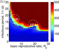
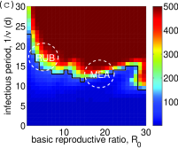
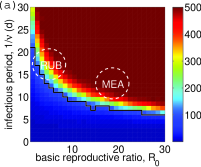
Figure 1: (Color online) The average length of simulations in years for 250 runs with the fixed length of 500 years. Below the black stairstep graph (the extinction boundary) all simulations went extinct within 500 years. In this region the time to extinction is below 200 years. In most of the region above the black line the average length of simulations is 500 years which means that none of the simulations went extinct and that the summary statistics of power spectra estimated from simulations are carried out on 250 runs. For points close to the extinction boundary the statistics are calculated on a variable number of runs. In practice, the spectra computed from as few as 30 runs are very smooth so that the sample size effects become negligible and the discrepancies between simulations and analytic predictions arise purely because of the breakdown of the theory [5, 10, 13]. This is seen from, for example, Figure 4 (b) in the main text which was computed from 30 runs (for parameters 2 points away from the extinction boundary). The sampling errors might appear only for parameters at the very border with the black line, where running long simulations becomes prohibitively computationally intensive. In that region few points may stand out from the general pattern as, for example, seen from the surface plots for amplification and coherence in Figures 3 and 5 of the main text. The same figures show that the dominant period is not affected by sampling. Parameters: $\mu=0.02$ 1/y, $N=10^{6}$, (a) $\epsilon=0$, (b) $\epsilon=0.05$ and (c) $\epsilon=0.1$.

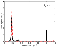
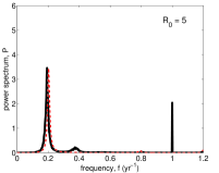
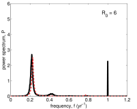
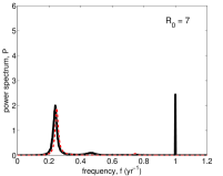
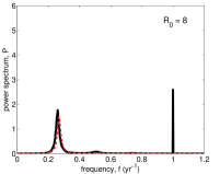
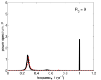
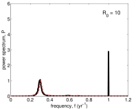
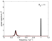
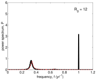
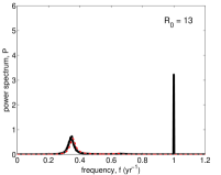
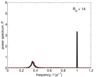
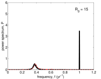
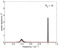
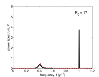
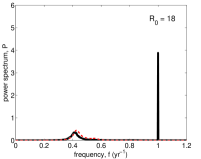
Figure 2: (Color online) Analytical spectra (dashed red lines) and full numerical spectra (solid black lines) for the seasonally forced model. Parameters: $\epsilon=0.05$, $\mu=0.02$ 1/y, $1/\nu=18$ d and $N=10^{6}$.

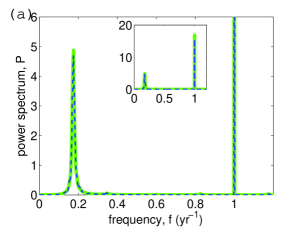
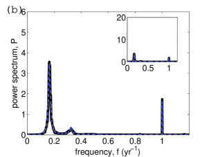
Figure 3: (Color online) Full numerical spectra for the model with sinusoidal forcing (solid green and black lines) and term-time forcing (dashed blue lines). The green and black lines are the same as in Figure 4 of the main text. In the term-time forced simulations we used $\beta(t)=\beta_{0}[1+\epsilon\text{Term}(t)]$, where $\text{Term}(t)$ is a periodic function that takes on value 1 during school terms and -1 during school holidays [8, 5]. The times of terms and holidays are taken from [8]. These define the fraction of time spent in school, $f=92/365$. The basic reproductive ratio is given by $R_{0}\approx\langle\beta\rangle/(\nu+\mu)$ [3, 8, 5], where $\langle\beta\rangle=\beta_{0}[(1+\epsilon)f+(1-\epsilon)(1-f)]$ is the time-averaged transmission rate. The perfect agreement between the spectra is achieved if the term-time forcing amplitude is 2.7 times larger than the sinusoidal forcing amplitude. This is consistent with the discussion in Ref [13] of [6] and in the Appendix B of [4]. Parameters: $\mu=0.02$ 1/y, $R_{0}=4$, $1/\nu=18$ d, $\epsilon=0.05$ (sinusoidal forcing, green and black lines), $\epsilon=0.135$ (term-time forcing, blue lines) (a) $N=10^{7}$ and (b) $N=10^{6}$.

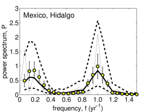
Figure 4: (Color online) Comparison of the full numerical spectrum of monthly incidence from simulations of the SIR model with seasonal forcing (yellow circles) and the spectrum obtained from the time series for Hidalgo, Mexico (lines). The lines are repeated from Figure 1 (d) of the main text. The simulated time series were 16 years long and sampled every month. The error bars correspond to the standard deviation for 20 simulations. In simulations we took $N=2100000$, the reporting rate of 0.01 [9] and $R_{0}=4$. This value of $R_{0}$ is slightly lower than that estimated in [9]. Its justification is two-fold: 1) the last years of the data time series correspond to post-vaccination and were not included in the analysis in [9]; 2) the lifespan, $1/\mu$, is likely to be longer than the one we used for all data sets in the main text because the Mexico data is more recent. Parameters: $\mu=0.02$ 1/y, $1/\nu=18$ d, $\epsilon=0.17$.

References

• [1] D.Β Alonso, A.Β J. McKane, and M.Β Pascual. Stochastic amplification in epidemics. Journal of the Royal Society Interface, 4:575–582, 2007.
• [2] D.Β F. Anderson. A modified next reaction method for simulating chemical systems with time dependent propensities and delays. Journal of Chemical Physics, 127:214107, 2007.
• [3] R.Β M. Anderson and R.Β M. May. Infectious diseases of humans. Oxford University Press, Oxford, OX2 6PD, 1991.
• [4] C.Β T. Bauch and D.Β J.Β D. Earn. Transients and attractors in epidemics. Proceedings of the Royal Society of London, Series B, 270:1573–1578, 2003.
• [5] A.Β J. Black and A.Β J. McKane. Stochastic amplification in an epidemic model with seasonal forcing. Journal of Theoretical Biology, 267:85–94, 2010.
• [6] D.Β J.Β D. Earn, P.Β Rohani, B.Β M. Bolker, and B.Β T. Grenfell. A simple model for complex dynamical transitions in epidemics. Nature, 287:667–670, 2000.
• [7] D.Β Gillespie. A general method for numerically simulating the stochastic time evolution of coupled chemical reactions. Journal of Computational Physics, 22:403–434, 1976.
• [8] M.Β J. Keeling, P.Β Rohani, and B.Β T. Grenfell. Seasonally forced disease dynamics explored as switching between attractors. Physica D, 148:317–335, 2001.
• [9] C.Β J.Β E. Metcalf, P.Β Klepac, M.Β Ferrari, N.Β Bharti, O.Β N. BjΓΈrnstad, and B.Β T. Grenfell. The epidemiology of rubella in Mexico: seasonality, stochasticity and regional variation. Epidemiology and Infection, 139:1029–1038, 2011.
• [10] G.Β Rozhnova and A.Β Nunes. Stochastic effects in a seasonally forced epidemic model. Physical Review E, 82:041906, 2010.
• [11] G.Β Rozhnova and A.Β Nunes. Modelling the long-term dynamics of pre-vaccination pertussis. Journal of the Royal Society Interface, 9:2959–2970, 2012.
• [12] G.Β Rozhnova, A.Β Nunes, and A.Β J. McKane. Stochastic oscillations in models of epidemics on a network of cities. Physical Review E, 84:051919, 2011.
• [13] M.Β SimΓ΅es, M.Β M. TeloΒ da Gama, and A.Β Nunes. Stochastic fluctuations in epidemics on networks. Journal of the Royal Society Interface, 5:555–566, 2008.
• [14] N.Β G. van Kampen. Stochastic Processes in Physics and Chemistry. Elsevier, Amsterdam, 1981.