Bayesian Group Nonnegative Matrix Factorization for EEG Analysis

Abstract

We propose a generative model of a group EEG analysis, based on appropriate kernel assumptions on EEG data. We derive the variational inference update rule using various approximation techniques. The proposed model outperforms the current state-of-the-art algorithms in terms of common pattern extraction. The validity of the proposed model is tested on the BCI competition dataset.

1 Introduction

Electroencephalography (EEG) is a multivariate time-series recording of electrical potentials induced by ionic flows among neurons in the brain. Since EEG has the highest temporal resolution among other non-invasive brain imaging techniques, it is widely used in the brain computer interface (BCI) research, especially on the applications where realtime capability is required, such as controlling a computer cursor [14], mobile robots [11], wheelchair [5, 13], and a humanoid robot [1]

There have been many approaches to classify mental state based on the preprocessed EEG signals. They include SVM [2], L1 regularized logistic regression [6], and nonnegative matrix factorization (NMF) [9]. According to [9], NMF based methods do not require any cross-validation in determining basis vectors which contain useful spectral traits in motor imagery EEG signals.

For each mental state, brain images consist of subject-dependent patterns and common patterns shared across multiple subjects. Most approaches proposed in the literature had not considered the latter. Since those methods can not capture common features occurring across all subjects, a pilot training phase is always required whenever a new subject comes to the system. To deal with this limitation, group-NMF [10] (GNMF) was proposed by modifying the cost functions of the standard NMF. The advantage of group analysis of EEG is twofold. First, it finds common patterns that can be used in the testing phase of other subjects without each pilot test, and second, it finds individual patterns that reflect intra-subject variability.

Most NMF algorithms, including GNMF, are based on optimization of the cost function under some constraints on the variables. Although non-generative models give more accurate results in general, we can not incorporate prior knowledge into them. It is well known that EEG data can be well represented with exponential distribution [15], but there is no mean to exploit this valuable information in the non-generative models of NMF. In addition, the non-generative models is not robust to the small size of data. while generative models are capable of embedding prior knowledge, and competitive performance can be achieved with little data.

With this motivation, we devise a generative mode of group EEG analysis, based on Bayesian nonnegative matrix factorization. We derive the variational inference update rule using various approximation techniques. The validity of the proposed model is tested on the BCI competition III dataset [3].

2 Model Description

We use preprocessed EEG signals applied power spectral density to have data matrix $X\in R^{l\times m\times n}$ for each subject $l$. Each $m$ dimension in $X$ represents frequency bin, and each $n$ dimension is associated with time stamp. In general, the NMF [12] finds a decomposition represented as $X=AS$. However, we assume two kinds of base matrices. One is common base matrix, $A_{C}\in R^{m\times k}$. It reflects activated regions and frequency kinds for a specific task class. And the other one is individual base, $A_{I}\in R^{l\times m\times j}$. The individual patterns vary depending on each subject, even though the task is the same. Hence we model $X$ as $X_{mnl}=\sum_{k=1}^{K}(A_{C})_{mk}(S_{C})_{lkn}+\sum_{j=1}^{J}(A_{I})_{lmj}(S_{I})_{ljn})$, where $S_{C}$ represents class indicator, and $S_{I}$ mixes individual factors appropriately. It is well known that EEG data can be well represented with exponential distribution [15], so we can construct a generative process as follows:

$$X_{mnl}|A_{C},(A_{I})_{l},(S_{C})_{l},(S_{I})_{l} \sim\textrm{Exponential}(\sum_{k=1}^{K}(A_{C})_{mk}(S_{C})_{lkn}+\sum_{j=1}^{J}(A_{I})_{lmj}(S_{I})_{ljn})$$

$$(A_{C})_{mk}|a \sim\textrm{Gamma}(a,a)$$

$$(A_{I})_{mkl}|b \sim\textrm{Gamma}(b,b)$$

$$(S_{C})_{lkn} =1(Y_{ln}=k)$$

$$(S_{I})_{ljn}|Y_{ln},c \sim\textrm{Gamma}(c_{Y_{ln}},c_{Y_{ln}})$$ (1)

Figure 1: Graphical Model for Bayesian NMF

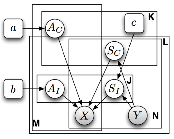
The graphical model for this is shown in Fig. 1. We assume gamma distribution for all priors, because we can have mathematical advantages of the inference algorithm, which is shown in Gap-NMF [7]. We design $A_{C}$ to have class specific image. Hence, we assume the number of common bases, $K$, is the same with the number of classes. The individual bases are designed to be dependent on a subject and a task class.

At the training phase, both $X$ and $Y$ are used as dataset to predict posterior of $A_{C},A_{I}$, while $X$ is the only available data in the testing (Note that we use the posterior of $A_{C},A_{I}$ predicted in the training phase). For a given estimated posterior of $A_{C}$,$A_{I}$, and test data $X^{test}$, we predict class label $Y^{test}$ as
$Y_{ln}^{test}=\underset{k}{\operatorname{arg\,max}}\,||X^{test}_{ln}-\hat{X_{ln}^{k}}||^{2},\,\,\hat{X_{ln}^{k}}=(A_{C})_{k}^{train}$

3 Variational Inference

There are two kinds of inference techniques in Bayesian graphical models, Markov Chain Monte Carlo (MCMC) and variational inference. Although MCMC is simple and easy to implement, it suffers from slow converge speed and no convergence guarantees. Therefore we derive variational inference algorithm of the proposed model.

We derive variational inference algorithms using the similar technique as introduced Gap-NMF [7] model. A typical mean-field variational inference uses the same distribution family as a variational distribution for each variable, but Hoffman et al. [7] showed that using Generalized Inverse-Gaussian (GIG) family [8] as a variational distribution gives tighter bound. Therefore we use GIG to approximate $q(A_{C})$ and $q(A_{I})$.

3.1 Lower Bound of the Marginal Likelihood

We can derive the lower bound of the marginal likelihood of $X$ after we factorize each variable fully.

$$\log p(X|a,b,c,Y) \geq E_{q}[\log p(X|A_{C},S_{C},A_{I},S_{I})]$$

$$+E_{q}[\log p(A_{C}|a)]+E_{q}[\log p(A_{I}|b)]+E_{q}[\log p(S_{I}|c,Y)]$$

$$-E_{q}[\log q(A_{C})]-E_{q}[\log q(A_{I})]-E_{q}[\log q(S_{I})]$$ (2)

The first term of the bound in (3.1) can be expanded to (3).

$$E_{q}[\log p(X|A_{C},S_{C},A_{I},S_{I})] =\sum_{lmn}\{E_{q}[\frac{-X_{lmn}}{\sum_{k}(A_{C})_{mk}(S_{C})_{lkn}+\sum_{j}(A_{I})_{lmj}(S_{I})_{ljn}}]$$ (3)

$$+E_{q}[-\log({\sum_{k}(A_{C})_{mk}(S_{C})_{lkn}+\sum_{j}(A_{I})_{lmj}(S_{I})_{ljn}})]\}$$

The first term in (3) can be approximated using Jensen’s inequality, because $-(\cdot)^{-1}$ is a concave function.

$$E_{q}[\frac{-X_{lmn}}{\sum_{k}(A_{C})_{mk}(S_{C})_{lkn}+\sum_{j}(A_{I})_{lmj}(S_{I})_{ljn}}]$$ (4)

$$\geq-\pi_{lnm1}^{2}X_{lmn}(\sum_{k}\phi_{lmnk}^{2}\frac{1}{(S_{C})_{lkn}}E_{q}[\frac{1}{(A_{C})_{mk}}])-\pi_{lnm2}^{2}X_{lmn}(\sum_{j}\psi_{lmnj}^{2}E_{q}[\frac{1}{(A_{I})_{lmj}(S_{I})_{ljn}}])$$

$$\pi_{lnm1}+\pi_{lnm2}=1,\,\,\sum_{k}\phi_{lmnk}=1,\,\,\sum_{j}\psi_{lmnj}=1$$

And for the second term in (3), we use the same method in [4], which gets lower bound of the convex function, $-\log x$, using a first order Taylor approximation.

$$E_{q}[-\log ({\sum_{k}(A_{C})_{mk}(S_{C})_{lkn}+\sum_{j}(A_{I})_{lmj}(S_{I})_{ljn}})]$$ (5)

$$\geq-\log w_{lmn}+1-\frac{1}{w_{lmn}}(\sum_{k}E_{q}[(A_{C})_{mk}](S_{C})_{lkn}+\sum_{j}E_{q}[(A_{I})_{lmj}(S_{I})_{ljn}])$$

3.2 Optimization

We present the optimization algorithm that maximizes the lower bound in (3.1), and it gives the approximated $p(A_{C})$ and $p(A_{I})$ through $Q(A_{C})$ and $Q(A_{I})$.

To optimize $\phi$, $\psi$, and $\pi$, we use Lagrange multipliers with sum-to-one constraints.

$$\phi_{lmnk} \propto(S_{C})_{lkn}E_{q}[\frac{1}{(A_{C})_{mk}}]^{-1},\,\,\,\,\psi_{lmnj}\propto E_{q}[\frac{1}{(A_{I})_{lmj}(S_{I})_{ljn}}]^{-1}$$

$$\pi_{lmn1} =\frac{\sum_{j}\psi_{lmnj}^{2}E_{q}[\frac{1}{(A_{I})_{lmj}(S_{I})_{ljn}}]}{\sum_{k}\phi_{mnk}^{2}E_{q}[\frac{1}{(A_{C})_{mk}(S_{C})_{lkn}}]+\sum_{j}\psi_{lmnj}^{2}E_{q}[\frac{1}{(A_{I})_{lmj}(S_{I})_{ljn}}]}$$ (6)

And for the inference of $w$ and other variational parameters, we use coordinate ascent algorithm to maximize the bound.

$$w_{lmn} =\sum_{k}E_{q}[(A_{C})_{mk}(S_{C})_{lkn}]+\sum_{j}E_{q}[(A_{I})_{lmj}(S_{I})_{ljn}]$$

$$\gamma_{(A_{C})_{mk}} =a,\,\,\,\,\rho_{(A_{C})_{mk}}=a+\sum_{ln}\frac{1}{w_{lmn}}(S_{C})_{lkn},\,\,\,\,\tau_{(A_{C})_{mk}}=\sum_{ln}\{\pi_{lnm1}^{2}X_{lmn}(\sum_{k}\phi_{lmnk}^{2}\frac{1}{(S_{C})_{lkn}})\}$$

$$\gamma_{(A_{I})_{lmj}} =b,\,\,\,\,\rho_{(A_{I})_{lmj}}=b+\sum_{n}\frac{1}{w_{lmn}}E_{q}[(S_{I})_{ljn}],\,\,\,\,\tau_{(A_{I})_{lmj}}=\sum_{n}\{\pi_{lmn2}^{2}X_{lmn}(\psi_{lmnj}^{2}E_{q}[\frac{1}{(S_{I})_{ljn}}])\}$$

$$\gamma_{(S_{I})_{ljn}} =c_{Y_{ln}},\,\,\,\,\rho_{(S_{I})_{ljn}}=c_{Y_{ln}}+\sum_{m}\frac{1}{w_{lmn}}E_{q}[(A_{I})_{lmj}],\,\,\,\,\tau_{(S_{I})_{ljn}}=\sum_{m}\{\pi_{lmn2}^{2}X_{lmn}(\psi_{lmnj}^{2}E_{q}[\frac{1}{(A_{I})_{lmj}}])\}$$ (7)

4 Experiments

We demonstrate the proposed model on the real EEG dataset. We compare our model to GNMF, the only group analysis model in the literature. The performance measure is the classification accuracy. Throughout the experiments we set all hyper parameters ($a,b,c_{1},c_{2}.c_{3}$) to 0.1, the number of common parameter to 3, and the number of individual parameter to 1.

4.1 IDIAP Dataset

The IDIAP Dataset [3] is comprised of precomputed features of EEG recorded from three subjects. Each subjects were asked to perform one of the three tasks for some duration of time. The tasks include imagination of left or right hand movements and generation of words beginning with the same random letter.

The preprocessing of the raw EEG is done by spatial filtering and power spectral density (PSD). The raw EEG has 8 centro-parietal channels, and PSD uses 12 frequency bins at every 62.5 ms, which constitutes the 96 dimensional feature vector.

4.2 Common and Individual Factor Extraction

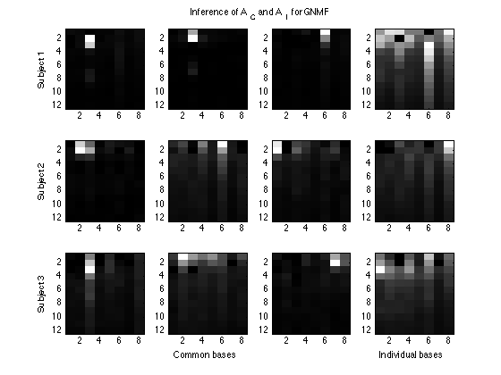
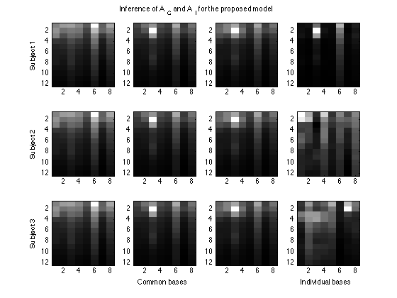
In neuroimaging, discovering subject independent patterns for a specific task is desirable, but intra subject variability often thwarts seeking them. If we can separate the two kinds of patterns, then the common activation patterns would be more clearly visible. In Fig. 2, we show a side-by-side comparison of the results of GNMF (Fig. 2(a)) and our proposed model (Fig. 2(b)) in terms of the separation of the common and individual bases. The common bases found by our model are in fact common patterns shared by all three subjects, whereas the common bases found by GNMF are not quite the same across the subjects. This shows that our model is better able to separate the common patterns from the individual patterns. Additionally, according to the results of the BCI competition, subject 1 showed the best performance, indicating that he was able to concentrate better on the task than subjects 2 and 3. Hence, we expect the individual pattern of subject 1 to be clearer (more concentrated in a small region) than those of subjects 2 and 3. The rightmost column of Fig. 2(b) shows the concentrated pattern around a small region for subject 1 and less concentrated patterns for subject 2 and subject3. On the other hand, GNMF does not reflect this individual performance difference in the individual bases in the rightmost column of in Fig. 2(a).

(a) Inference of bases of GNMF

(b) Inference of bases of the proposed model

Figure 2: According to the result of the BCI competition III, the best performance was achieved in subject 1, which means he or she is less distracted. Likewise, the subject 3 is more distracted than subject 2. This fact is well reflected in the proposed model, (b)

4.3 Sensitivity of the Training Data Size

Figure 3: Performance comparison under various training data size for each subject

In general, the performance of a Bayesian graphical model is less sensitive to the size of training data because it can take advantage of the prior. The proposed model inherits this advantage, so the performance is robust to the size of the training data. In practice, a smaller training dataset is desirable if it can achieve comparable performance because gathering of training data often costs time and money. Fig. 3 shows such robustness of our model. Note that our model performs well with only the common bases (except the subject 3). This shows that while our model captures the common patterns well, it does not capture the individual patterns well. This shows the limitation of our model in its current form and shows potential for better performance once the model can also capture the individual variability.

5 Conclusion

We presented a generative model for analyzing group EEG data. The proposed models finds common patterns for a specific task class across all subjects as well as individual patterns that capture intra-subject variability. The proposed model seems to capture the common patterns better than previously proposed group NMF model, and it seems less sensitive to the size of the training data because it is a generative model. However, the limitation of the model is that it does not model the individual variability well, and that is left for future research. We believe that better modeling the individual variability, combined with the good performance for common pattern discovery, will result in an overall improved model.

References

- [1] Bell, C., Shenoy, P., Chalodhorn, R., Rao, R.: Control of a humanoid robot by a noninvasive brain–computer interface in humans. Journal of Neural Engineering 5(2), 214 (2008)
- [2] Blankertz, B., Curio, G., Muller, K.: Classifying single trial eeg: Towards brain computer interfacing. Advances in neural information processing systems 1, 157–164 (2002)
- [3] Blankertz, B., Muller, K., Krusienski, D., Schalk, G., Wolpaw, J., Schlogl, A., Pfurtscheller, G., Millan, J., Schroder, M., Birbaumer, N.: The bci competition iii: Validating alternative approaches to actual bci problems. Neural Systems and Rehabilitation Engineering, IEEE Transactions on 14(2), 153–159 (2006)
- [4] Blei, D., Lafferty, J.: Correlated topic models. Advances in neural information processing systems 18, 147 (2006)
- [5] Galán, F., Nuttin, M., Lew, E., Ferrez, P., Vanacker, G., Philips, J., Millán, J.: A brain-actuated wheelchair: asynchronous and non-invasive brain–computer interfaces for continuous control of robots. Clinical Neurophysiology 119(9), 2159–2169 (2008)
- [6] Grosse-Wentrup, M., Liefhold, C., Gramann, K., Buss, M.: Beamforming in noninvasive brain–computer interfaces. Biomedical Engineering, IEEE Transactions on 56(4), 1209–1219 (2009)
- [7] Hoffman, M.D., Blei, D.M., Cook, P.R.: Bayesian nonparametric matrix factorization for recorded music. Proc. ICML pp. 641–648 (2010)
- [8] Jørgensen, B.: Statistical properties of the generalized inverse Gaussian distribution, vol. 21. Springer New York (1982)
- [9] Lee, H., Cichocki, A., Choi, S.: Nonnegative matrix factorization for motor imagery eeg classification. Artificial Neural Networks–ICANN 2006 pp. 250–259 (2006)
- [10] Lee, H., Choi, S.: Group nonnegative matrix factorization for EEG classification. International Conference on Artificial Intelligence and Statistics (2009)
- [11] Millan, J., Renkens, F., Mouriño, J., Gerstner, W.: Noninvasive brain-actuated control of a mobile robot by human eeg. Biomedical Engineering, IEEE Transactions on 51(6), 1026–1033 (2004)
- [12] Seung, D., Lee, L.: Algorithms for non-negative matrix factorization. Advances in neural information processing systems 13, 556–562 (2001)
- [13] Shin, B., Kim, T., Jo, S.: Non-invasive brain signal interface for a wheelchair navigation. In: Control Automation and Systems (ICCAS), 2010 International Conference on. pp. 2257–2260. IEEE (2010)
- [14] Wolpaw, J., McFarland, D.: Control of a two-dimensional movement signal by a noninvasive brain-computer interface in humans. Proceedings of the National Academy of Sciences of the United States of America 101(51), 17849–17854 (2004)
- [15] Zaveri, H., Williams, W., Iasemidis, L., Sackellares, J.: Time-frequency representation of electrocorticograms in temporal lobe epilepsy. Biomedical Engineering, IEEE Transactions on 39(5), 502–509 (1992)