Prediction of Parallel Speed-ups for Las Vegas Algorithms

Abstract

We propose a probabilistic model for the parallel execution of Las Vegas algorithms, i.e., randomized algorithms whose runtime might vary from one execution to another, even with the same input. This model aims at predicting the parallel performances (i.e., speedups) by analysis the runtime distribution of the sequential runs of the algorithm. Then, we study in practice the case of a particular Las Vegas algorithm for combinatorial optimization, on three classical problems, and compare with an actual parallel implementation up to 256 cores. We show that the prediction can be quite accurate, matching the actual speedups very well up to 100 parallel cores and then with a deviation of about 20% up to 256 cores.

heory, Algorithms, Performance.

1 Introduction

We will consider in this paper Las Vegas algorithms, introduced a few decades ago by Babai [1979], i.e. randomized algorithms whose runtime might vary from one execution to another, even with the same input. An important class of Las Vegas algorithms is the family of Stochastic Local Search methods Hoos and Stütze [2005]. They have been used in Combinatorial Optimization for finding optimal or near-optimal solutions for several decades Aarts and Lenstra [1997], stemming from the pioneering work of Lin on the Traveling Salesman Problem Lin [1965]. Theses methods are now widely used in combinatorial optimization to solve real-life problems when the search space is too large to be explored by complete search algorithm, such as Mixed Integer Programming or Constraint Solving, c.f. Gonzalez [2007].

In the last years, several proposal for implementing local search algorithms on parallel computer have been proposed, the most popular being to run several competing instances of the algorithms on different cores, with different initial conditions or parameters, and let the fastest process win over others. We thus have an algorithm with the minimal execution time among the launched processes. This lead to so-called independent multi-walk algorithms in the local search community Verhoeven and Aarts [1995] and portfolio algorithms in the SAT community (satisfiability of Boolean formula) Gomes and Selman [2001]. This parallelization scheme can of course be generalized to any Las Vegas algorithm.

The goal of this paper is to study the parallel performances of Las Vegas algorithms under this independent multi-walk scheme, and to predict the performances of the parallel execution from the runtime distribution of the sequential runs of a given algorithm. We will confront these predictions with actual speedups obtained for a parallel implementation of a local search algorithm and show that the prediction can be quite accurate, matching the actual speedup very well up to 100 parallel cores and then with a deviation limited to about 20% up to 256 cores.

The paper is organized as follows. Section 2 is devoted to present the definition of Las Vegas algorithms, their parallel multi-walk execution scheme, and the main idea for predicting the parallel speedups. Section 3 will detail the probabilistic model of Las Vegas algorithms and their parallel execution scheme. Section 4 will present the example of local search algorithms for combinatorial optimization, while Section 5 will detail the benchmark problems and the sequential performances. Then, Section 6 will apply the general probabilistic model to the benchmark results and thus predict their parallel speedup, which will be compared to actual speedups of a parallel implementation in Section 7. A short conclusion and future work end will the paper.

2 Preliminaries

2.1 Las Vegas Algorithms

We borrow the following definition from Hoos and Stütze [2005], Chapter 4.

Definition 1 (Las Vegas Algorithm).

An algorithm A for a problem class $\Pi$ is a (generalized) Las Vegas algorithm if and only if it has the following properties:

1. If for a given problem instance $\pi\in\Pi$, algorithm A terminates returning a solution $s$, $s$ is guaranteed to be a correct solution of $\pi$.

2. For any given instance $\pi\in\Pi$, the run-time of A applied to $\pi$ is a random variable.

This is a slight generalization of the classical definition, as it includes algorithms which are not guaranteed to return a solution.

A large class of Las Vegas algorithms is the so-called family of metaheuristics, such as Simulated Annealing, Genetic Algorithms, Tabu Search, Swarm Optimization, Ant-Colony optimization, etc, which have been applied to different sets of problems ranging from resource allocation, scheduling, packing, layout design, frequency allocation, etc.

2.2 Multi-walk Parallel Extension

Parallel implementation of local search metaheuristics Gonzalez [2007]; Ibaraki et al. [2005] has been studied since the early 1990s, when parallel machines started to become widely available Pardalos et al. [1995]; Verhoeven and Aarts [1995]. With the increasing availability of PC clusters in the early 2000s, this domain became active again Alba [2004]; Crainic and Toulouse [2002]. Apart from domain-decomposition methods and population-based method (such as genetic algorithms), Verhoeven and Aarts [1995] distinguishes between single-walk and multi-walk methods for Local Search. Single-walk methods consist in using parallelism inside a single search process, e.g., for parallelizing the exploration of the neighborhood (see for instance Van Luong et al. [2010] for such a method making use of GPUs for the parallel phase). Multi-walk methods (parallel execution of multi-start methods) consist in developing concurrent explorations of the search space, either independently or cooperatively with some communication between concurrent processes. Sophisticated cooperative strategies for multi-walk methods can be devised by using solution pools Crainic et al. [2004], but require shared-memory or emulation of central memory in distributed clusters, thus impacting on performance. A key point is that a multi-walk scheme is easier to implement on parallel computers without shared memory and can lead, in theory at least, to linear speedups Verhoeven and Aarts [1995]. However this is only true under certain assumptions and we will see that we need to develop a more realistic model in order to cope with the performance actually observed in parallel executions.

Let us now formally define a parallel multi-walk Las Vegas algorithm.

Definition 2 (Multi-walk Las Vegas Algorithm).

An algorithm A’ for a problem class $\Pi$ is a (parallel) multi-walk Las Vegas algorithm if and only if it has the following properties:

1. It consists of $n$ instances of a sequential Las Vegas algorithm A for $\Pi$, say $A_{1},...,A_{n}$.

2. If, for a given problem instance $\pi\in\Pi$, there exists at least one $i\in[1,n]$ such that $A_{i}$ terminates, then let $A_{m},m\in[1,n]$, be the instance of A terminating with the minimal runtime and let $s$ be the solution returned by $A_{m}$. Then algorithm A’ terminates in the same time as $A_{m}$ and returns solution $s$.

3. If, for a given problem instance $\pi\in\Pi$, all $A_{i},i\in[1,n]$, do not terminate then A’ does not terminate.

2.3 How to Estimate Parallel Speedup ?

The multi-walk parallel scheme is rather simple, yet it provides an interesting test-case to study how Las Vegas algorithms can scale-up in parallel. Indeed runtime will vary among the processes launched in parallel and the overall runtime will be that of the instance with minimal execution time (i.e. ”long” runs are killed by ”shorter” ones). The question is thus to quantify the (relative) notion of short and long runs and their probability distribution. This might gives us a key to quantify the expected parallel speed-up. Obviously, this can be observed from the sequential behavior of the algorithm, and more precisely from the proportion of long and short runs in the sequential runtime distribution.

In the following, we propose a probabilistic model to quantify the expected speed-up of multi-walk Las Vegas algorithms. This makes it possible to give a general formula for the speed-up, depending on the sequential behavior of the algorithm. Our model is related to order statistics, a rather new domain of statistics David and Nagaraja [2003], which is the statistics of sorted random draws. Indeed, explicit formulas have been given for several well-known distributions. Relying on an approximation of the sequential distribution, we compute the average speed-up for the multi-walk extension. Experiments show that the prediction is quite good and opens the way for defining more accurate models and apply them to larger classes of algorithms.

Previous works Verhoeven and Aarts [1995] studied the case of a particular distribution for the sequential algorithm, the exponential distribution. This case is ideal and the best possible, as it yields a linear speed-up. Our model makes it possible to approximate Las Vegas algorithms by other types of distribution, such as a shifted exponential distribution or a lognormal distribution. In the last two cases the speed-up is no longer linear, but admits a finite limit when the number of processors tends toward infinity. We will see that it fits experimental data for some problems.

3 Probabilistic Model

Local Search algorithms are stochastic processes. They include several random components: choice of an initial configuration, choice of a move among several candidates, plateau mechanism, random restart, etc. In the following, we will consider the computation time of an algorithm (whatever it is) as a random variable, and use elements of probability theory to study its multi-walk parallel version. Notice that the computation time is not necessarily the cpu-time; it can also be the number of iterations performed during the execution of the algorithm.

3.1 Min Distribution

Consider a given algorithm on a given problem of a given size, say, the Magic-Square $10\times 10$. Depending on the result of some random components inside the algorithm, it may find a solution after $0$ iterations, $10$ iterations, or $10^{6}$ iterations. The number of iterations of the algorithm is thus a discrete random variable, let’s call it $Y$, with values in $\mathbb{N}$. $Y$ can be studied through its cumulative distribution, which is by definition, the function $\mathcal{F}_{Y}$ s.t. $\mathcal{F}_{Y}(x)=\mathbb{P}[Y\leq x]$, or by its distribution, which is by definition the derivative of $\mathcal{F}_{Y}$: $f_{Y}=\mathcal{F}_{Y}^{\prime}$.

It is often more convenient to consider distributions with values in $\mathbb{R}$ because it makes calculations easier. For the same reason, although $f_{Y}$ is defined in $\mathbb{N}$, we will use its natural extension to $\mathbb{R}$. The expectation of the computation is then defined as $\mathbb{E}[Y]=\int_{0}^{\infty}tf_{Y}(t)dt$

Assume that the base algorithm is concurrently run in parallel on $n$ cores. In other words, over each core the running process is a fork of the algorithm. The first process which finds a solution then kills all others. and the algorithm terminates. The $i$-th process corresponds to a draw of a random variable $X_{i}$, following distribution $f_{Y}$. The variables $X_{i}$ are thus independently and identically distributed (i.i.d.). The computation time of the whole parallel process is also a random variable, let $Z^{(n)}$, with a distribution $f_{Z^{(n)}}$ that depends both on $n$ and on $f_{Y}$. Since all the $X_{i}$ are i.i.d., the cumulative distribution $\mathcal{F}_{Z^{(n)}}$ can be computed as follows:

$$\mathcal{F}_{Z^{(n)}} = \mathbb{P}[Z^{(n)}\leq x]$$

$$= \mathbb{P}[\exists i\in\{1...n\},X_{i}\leq x]$$

$$= 1-\mathbb{P}[\forall i\in\{1...n\},X_{i}>x]$$

$$= 1-\prod_{i=1}^{n}\mathbb{P}[X_{i}>x]$$

$$= 1-\left(1-\mathcal{F}_{Y}(x)\right)^{n}$$

which leads to:

$$f_{Z^{(n)}} = \left(1-(1-\mathcal{F}_{Y}\right)^{n})^{\prime}$$

$$= nf_{Y}(1-\mathcal{F}_{Y})^{n-1}$$

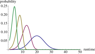
Thus, knowing the distribution for the base algorithm $Y$, one can calculate the distribution for $Z^{(n)}$. In the general case, the formula shows that the parallel algorithm favors short runs, by killing the slower processes. Thus, we can expect that the distribution of $Z^{(n)}$ moves toward the origin, and is more peaked. As an example, Figure 1 shows this phenomenon when the base algorithm admits a gaussian distribution.

Figure 1: Distribution of $Z^{(n)}$, in the case where $Y$ admits a gaussian distribution (cut on $\mathbb{R}^{-}$ and renormalized). The blue curve is $Y$. The distributions of $Z^{(n)}$ are in pink for $n=10$, in yellow for $n=100$ and in green for $n=1000$.

3.2 Expectation and Speed-up

The model described above gives the probability distribution of a parallelized version of any random algorithm. We can now calculate the expectation for the parallel process with the following relation:

$$\mathbb{E}[Z^{(n)}] = \int_{0}^{\infty}tf_{Z^{(n)}}(t)dt$$

$$= n\int_{0}^{\infty}tf_{Y}(t)(1-\mathcal{F}_{Y}(t))^{n-1}dt$$

Unfortunately, this does not lead to a general formula for $\mathbb{E}[Z^{(n)}]$. In the following, we will study it for different specific distributions.

To measure the gain obtained by parallelizing the algorithm on $n$ core, we will study the speed-up $\mathcal{G}_{n}$ defined as:

$$\mathcal{G}_{n}=\mathbb{E}[Y]/\mathbb{E}[Z^{(n)}]$$

Again, no general formula can be computed and the expression of the speed-up will depend on the distribution of $Y$.

However, it is worth noting that our computation of the speed-up is related to order statistics, see David and Nagaraja [2003] for a detailed presentation. For instance, the first order statistics of a distribution is its minimal value, and the $k^{th}$ order statistic is its $k^{th}$-smallest value. For predicting the speedup, we are indeed interested in computing the expectation of the distribution of the minimum draw. As the above formula suggests, this may lead to heavy calculations, but recent studies such as Nadarajah [2008] give explicit formulas for this quantity for several classical probability distributions.

3.3 Case of an Exponential Distribution

Assume that $Y$ has a shifted exponential distribution, as it has been suggested by Aiex et al. [2002, 2007].

$$f_{Y}(t)= \left\{\begin{array}[]{l l}0&\text{ if }t<x_{0}\\ \lambda e^{-\lambda(t-x_{0})}&\text{ if }t>x_{0}\\ \end{array}\right.$$

$$\mathcal{F}_{Y}(t)= \left\{\begin{array}[]{l l}0&\text{ if }t<x_{0}\\ 1-e^{-\lambda(t-x_{0})}&\text{ if }t>x_{0}\\ \end{array}\right.$$

$$\mathbb{E}[Y]= x_{0}+1/\lambda$$

Then the above formula can be symbolically computed by hand:

$$f_{Z^{(n)}}(t)= \left\{\begin{array}[]{l l}0&\text{ if }t<x_{0}\\ n\lambda e^{-n\lambda(t-x_{0})}&\text{ if }t>x_{0}\\ \end{array}\right.$$

$$\mathcal{F}_{Z^{(n)}}(t)= \left\{\begin{array}[]{l l}0&\text{ if }t<x_{0}\\ 1-e^{-n\lambda(t-x_{0})}&\text{ if }t>x_{0}\\ \end{array}\right.$$

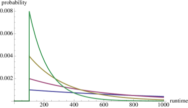
The intuitive observation of section 3.1 is easily seen on the expression of the parallel distribution, which has an initial value multiplied by $n$ but an exponential factor decreasing $n$-times faster, as shown on the curves of Figure 2.

Figure 2: For an exponential distribution, here in blue with $x_{0}=100$ and $\lambda=1/1000$, simulations of the distribution of $Z^{(n)}$for $n=2$ (pink), $n=4$ (yellow) and $n=8$ (green).

And in this case, one can symbolically compute both the expectation and speed-up for $Z^{(n)}$:

$$\mathbb{E}[Z^{(n)}] = n\lambda\int_{x_{0}}^{\infty}te^{-n\lambda(t-x_{0})}dt$$

$$= x_{0}+\frac{1}{n\lambda}$$

$$\mathcal{G}_{n} = \frac{x_{0}+\frac{1}{\lambda}}{x_{0}+\frac{1}{n\lambda}}$$

Figure 3 shows the evolution of the speed-up when the number of cores increases. With such a rather simple formula for the speed-up, it is worth studying what happens when the number of cores $n$ tends to infinity. Depending on the chosen algorithm, $x_{0}$ may be null or not. If $x_{0}=0$, then the expectation tends to $0$ and the speed-up is equal to $n$. This case has already been studied by Verhoeven and Aarts [1995]. For $x_{0}>0$, the speed-up admits a finite limit which is $\frac{x_{0}+\frac{1}{\lambda}}{x_{0}}=1+\frac{1}{x_{0}\lambda}$. Yet, this limit may be reached slowly, but depends on the value of $x_{0}$ and $\lambda$: obviously, the closest $x_{0}$ is to zero and the higher it will be. Another interesting value is the coefficient of the tangent at the origin, which approximates the speed-up for a small number of cores. In case of an exponential, it is $(x_{0}*\lambda+1)$. The higher $x_{0}$ and $\lambda$, the bigger is the speed-up at the beginning. In the following, we will see that, depending on the combinations of $x_{0}$ and $\lambda$, different behaviors can be observed.

Figure 3: Predicted speed-up in case of an exponential distribution, with $x_{0}=100$ and $\lambda=1/1000$, w.r.t. the number of cores.

3.4 Case of a Lognormal Distribution

Other distributions can be considered, depending on the behavior of the base algorithm. We will study the case of a lognormal distribution, which is the log of a gaussian distribution, because it will be shown in Section 6.2 that it fits one experiment. It has two parameters, the mean $\mu$ and the standard deviation $\sigma$. In the same way as the shifted exponential, we shift the distribution so that it starts at a given parameter $x_{0}$. Formally, a (shifted) lognormal distribution is defined as:

$$f_{Y}(t)= \left\{\begin{array}[]{l l}0&\text{ if }t<x_{0}\\ \frac{e^{-\frac{(-\mu+log(t-x_{0}))^{2}}{2\sigma^{2}}}}{\sqrt{2\pi}(t-x_{0})\sigma}&\text{ if }t>x_{0}\\ \end{array}\right.$$

$$\mathcal{F}_{Y}(t)= \left\{\begin{array}[]{l l}0&\text{ if }t<x_{0}\\ \frac{1}{2}\text{erfc}(\frac{\mu-log(t-x_{0})}{\sqrt{2}\sigma})&\text{ if }t>x_{0}\\ \end{array}\right.$$

where erfc is the complementary error function defined by $\text{erfc}(z)=\frac{2}{\sqrt{\pi}}\int_{z}^{\infty}e^{-t^{2}}dt$.

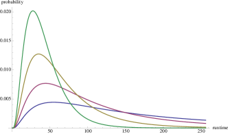
Figure 4 depicts lognormal distributions of $Z^{(n)}$, for several $n$. The computations for the distribution of $Z^{(n)}$, its expectation and the theoretical speed-up are quite complicated formulas. But Nadarajah [2008] gives an explicit formula for all the moments of lognormal order statistics with only a numerical integration step, from which we can derive a computation of the speed-up (since the expectation of $Z^{(n)}$is the first order moment for the first order statistics). This allows us to draw the general shape of the speed-up, an example being given on Figure 5. Due to the numerical integration step, which requires numerical values for the number of cores $n$, we restrict the computation to integer values of $n$. This is a reasonable limitation as the number of cores is indeed an integer.

Figure 4: For a lognormal distribution, here in blue with $x_{0}=0$, $\mu=5$ and $\sigma=1$, simulations of the distribution of $Z^{(n)}$for $n=2$ (pink), $n=4$ (yellow) and $n=8$ (green).

Figure 5: Predicted speed-up in case of a lognormal distribution, with $x_{0}=0$, $\mu=5$ and $\sigma=1$, depending on the number of cores (on the abscissa).

4 Application to Local Search

Since about a decade, the interest for the family of Local Search methods and Metaheuristics for solving large combinatorial problems has been growing and has attracted much attention from both the Operations Research and the Artificial Intelligence communities for solving real-life problems Gonzalez [2007]; Hentenryck and Michel [2005]; Ibaraki et al. [2005].

4.1 Local Search for Constraint Solving

Local Search starts from a random configuration and tries to improve this configuration, little by little, through small changes in the values of the problem variables. Hence the term “local search” as, at each time step, only new configurations that are “neighbors” of the current configuration are explored. The definition of what constitutes a neighborhood will of course be problem-dependent, but basically it consists in changing the value of a few variables only (usually one or two). The advantage of Local Search methods is that they will usually quickly converge towards a solution (if the optimality criterion and the notion of neighborhood are defined correctly…) and not exhaustively explore the entire search space.

Applying Local Search to Constraint Satisfaction Problems (CSP) has been attracting some interest since about a decade Codognet and Diaz [2001]; Galinier and Hao [2000]; Hentenryck and Michel [2005], as it can tackle CSPs instances far beyond the reach of classical propagation-based constraint solvers Hentenryck [1989]; Bessiere [2006]. A generic, domain-independent constraint-based local search method, named Adaptive Search, has been proposed by Codognet and Diaz [2001, 2003]. This meta-heuristic takes advantage of the structure of the problem in terms of constraints and variables and can guide the search more precisely than a single global cost function to optimize, such as for instance the number of violated constraints. The algorithm also uses a short-term adaptive memory in the spirit of Tabu Search in order to prevent stagnation in local minima and loops.

4.2 Adaptive Search

An implementation of Adaptive Search (AS) has been developed in C language as a framework library and is available as a freeware at the URL:
http://cri-dist.univ-paris1.fr/diaz/adaptive/

We used this reference implementation for our experiments. The Adaptive Search method can be applied to a large class of constraints (e.g. linear and non-linear arithmetic constraints, symbolic constraints, etc.) and naturally copes with over-constrained problems Truchet [2004]. The input of the method is a Constraint Satisfaction Problem (CSP for short), which is defined as a triple (X;D;C), where X is a set of variables, D is a set of domains, i.e., finite sets of possible values (one domain for each variable), and C a set of constraints restricting the values that the variables can simultaneously take. For each constraint, an error function needs to be defined; it gives, for each tuple of variable values, an indication of how much the constraint is violated. This idea has also been proposed independently by Galinier and Hao [2000], where it is called “penalty functions”, and then reused by the Comet system Hentenryck and Michel [2005], where it is called “violations”. For example, the error function associated with an arithmetic constraint $|X-Y|<c$, for a given constant $c\geq 0$, can be $max(0,|X-Y|-c)$.

Adaptive Search relies on iterative repair, based on variable and constraint error information, seeking to reduce the error on the worst variable so far. The basic idea is to compute the error function for each constraint, then combine for each variable the errors of all constraints in which it appears, thereby projecting constraint errors onto the relevant variables. This combination of errors is problem-dependent, see Codognet and Diaz [2001] for details and examples, but it is usually a simple sum or a sum of absolute values, although it might also be a weighted sum if constraints are given different priorities. Finally, the variable with the highest error is designated as the “culprit” and its value is modified. In this second step, the well known min-conflict heuristic Minton et al. [1992] is used to select the value in the variable domain which is the most promising, that is, the value for which the total error in the next configuration is minimal.

In order to prevent being trapped in local minima, the Adaptive Search method also includes a short-term memory mechanism to store configurations to avoid (variables can be marked Tabu and “frozen” for a number of iterations). It also integrates reset transitions to escape stagnation around local minima. A reset consists in assigning fresh random values to some variables (also randomly chosen). A reset is guided by the number of variables being marked Tabu. It is also possible to restart from scratch when the number of iterations becomes too large (this can be viewed as a reset of all variables but it is guided by the number of iterations). The core ideas of adaptive search can be summarized as follow:

• to consider for each constraint a heuristic function that is able to compute an approximated degree of satisfaction of the goals (the current error on the constraint);

• to aggregate constraints on each variable and project the error on variables thus trying to repair the worst variable with the most promising value;

• to keep a short-term memory of bad configurations to avoid looping (i.e. some sort of tabu list) together with a reset mechanism.

5 Benchmark Problems and Experimental Results

We have chosen to test this method on two problems from the CSPLib benchmark library Gent and Walsh [1999], and on a hard combinatorial problem abstracted from radar and sonar applications. After briefly introducing the classical benchmarks, we detail the latter problem, called Costas Array. Then we show the performance and the speed-ups obtained with both sequential and a multi-walk Adaptive Search algorithm on these problems.

We use two classical benchmarks from CSPLib consisting of:

• The All-Interval Series problem (prob007 in CSPLib),

• The Magic-Square problem (prob019 in CSPLib).

Although these benchmarks are academic, they are abstractions of real-world problems and could involve very large combinatorial search spaces, e.g., the 200$\times$200 Magic-Square problem requires 40,000 variables whose domains range over 40,000 values. Indeed the search space in the Adaptive Search model (using permutations) is $40,000!$, i.e., more than $10^{166713}$ configurations. Classical propagation-based constraint solvers cannot solve this problem for instances higher than 20x20. Also note that we are tackling constraint satisfaction problems as optimization problems, that is, we want to minimize the global error (representing the violation of constraints) to value zero, therefore finding a solution means that we actually reach the bound (zero) of the objective function to minimize.

5.1 The All-Interval Series Problem

This problem is described as prob007 in the CSPLib. This benchmark is in fact a well-known exercise in music Truchet and Codognet [2004] where the goal is to compose a sequence of $N$ notes such that all are different and tonal intervals between consecutive notes are also distinct. This problem is equivalent to finding a permutation of the $N$ first integers such that the absolute difference between two consecutive pairs of numbers are all different. This amounts to finding a permutation $(X1,\ldots X_{N})$ of $\{0,\ldots N-1\}$ such that the list $(abs(X_{1}-X_{2}),abs(X_{2}-X_{3})\ldots abs(X_{N-1}-x_{N}))$ is a permutation of ${1,\ldots,N-1}$. A possible solution for $N=8$ is $(3,6,0,7,2,4,5,1)$ since all consecutive distances are different:

3 $\frac{3}{~{}~{}~{}~{}}$ 6 $\frac{6}{~{}~{}~{}~{}}$ 0 $\frac{7}{~{}~{}~{}~{}}$ 7 $\frac{5}{~{}~{}~{}~{}}$ 2 $\frac{2}{~{}~{}~{}~{}}$ 4 $\frac{1}{~{}~{}~{}~{}}$ 5 $\frac{4}{~{}~{}~{}~{}}$ 1

5.2 The Magic-Square Problem

The Magic-Square problem is catalogued as prob019 in CSPLib and consists in placing the numbers $\{1,2\cdots N^{2}\}$ on an $N\times N$ square such that each row, column and main diagonal equal the same sum (the constant $N(N^{2}+1)/2$).

For instance, this figure shows a well-known solution for $N=4$ (depicted by Albrecht Dürer in his engraving Melancholia I, 1514).

5.3 The Costas Array Problem

A Costas array is an $N\times N$ grid containing $N$ marks such that there is exactly one mark per row and per column and the $N(N-1)/2$ vectors joining the marks are all different. We give here an example of Costas array of size 5. It is convenient to see the Costas Array Problem (CAP) as a permutation problem by considering an array of $N$ variables $(V_{1},\ldots,V_{N})$ which forms a permutation of $\{1,2,\ldots,N\}$. The above Costas array can thus be represented by the array $[3,4,2,1,5]$.

Historically these arrays have been developed in the 1960’s to compute a set of sonar and radar frequencies avoiding noise Costas [1984]. A very complete survey on Costas arrays can be found in Drakakis [2006]. The problem of finding a Costas array of size $N$ is very complex since the required time grows exponentially with $N$. In the 1980’s, several algorithms have been proposed to build a Costas array given $N$ (methods to produce Costas arrays of order 24 to 29 can be found in Beard et al. [2007]; Drakakis et al. [2011a, b]; Russo et al. [2010]), such as the Welch construction Golomb [1984] and the Golomb construction Golomb and Taylor [1984], but these methods cannot built Costas arrays of size $32$ and some higher non-prime sizes. Nowadays, after many decades of research, it remains unknown if there exist any Costas arrays of size $32$ or $33$. Another difficult problem is to enumerate all Costas arrays for a given size. Using the Golomb and Welch constructions, Drakakis et. al present in Drakakis et al. [2011b] all Costas arrays for $N=29$. They show that among the $29!$ permutations, there are only 164 Costas arrays, and 23 unique Costas arrays up to rotation and reflection.

5.4 Sequential Results

We run our benchmarks in a sequential manner in order to have about 650 runtimes for each. Sequential experiments, as well as parallel experiments, have been done on the Griffon cluster of the Grid’5000 platform. The following Tables 1 and 2 shows the minimum, mean, median and maximum respectively among the runtimes and the number of iterations of our benchmarks.

Problem	Min	Mean	Median	Max
MS 200	5.51	382.0	126.3	7,441.6
AI 700	23.25	1,354.0	945.4	10,243.4
Costas 21	6.55	3,744.4	2,457.4	19,972.0

Table 1: Sequential execution times (in seconds)

Problem	Min	Mean	Median	Max
MS 200	6,210	443,969	164,042	7,895,872
AI 700	1,217	110,393	76,242	826,871
Costas 21	321,361	183,428,617	119,667,588	977,709,115

Table 2: Sequential number of iterations

One can see that runtimes and the number of iterations, respectively from Tables 1 and 2, are spread over a large interval, illustrating the stochasticity of the algorithm. Depending on the benchmark, there is a ratio of a few thousands between the minimum and the maximum runtimes.

5.5 Parallel Results

We have conduct parallel experiments on the Grid5000 platform Bolze and al. [2006], the French national grid for research, which contains 8,596 cores deployed on 11 sites distributed in France. For our experiments, we used the Griffon cluster at Nancy, composed of 184 Intel Xeon L5420 (Quad-core, 2.5GHz, 12MB of L2-cache, bus frequency at 1333MHz), thus with a total of 736 cores available giving a peak performances of 7.36TFlops.

Tables 3 and 4 present the execution times and the number of iterations, respectively, with speed-ups for executions of large benchmarks Magic-Square 200$\times$200, All-Interval with $n$ = 700 and Costas Array with $n=21$, up to 256 cores. The same code has been ported and executed, timings are given in seconds and are the average of 50 runs. One can notice there are no significant differences between speed-ups of these two tables, therefore we will prefer as a time measurement the number of iterations, which has the good property of not being machine-dependent. Anyway, similar speed-ups have been achieved on other parallel machines Caniou et al. [2012].

Problem	time on 1 core	speed-up on $k$ cores
	(seconds)	16	32	64	128	256
MS 200	382.0	18.3	24.5	32.3	37.0	47.8
AI 700	1,354.0	12.9	19.3	30.6	39.2	45.5
Costas 21	3,744.4	15.7	26.4	59.8	154.5	274.8

Table 3: Speed-ups with respect to sequential time

Problem	# of iterations	speed-up on $k$ cores
	on 1 core	16	32	64	128	256
MS 200	443,969	16.6	22.2	29.9	34.3	45.0
AI 700	110,393	12.8	20.2	29.3	37.3	48.0
Costas 21	183,428,617	15.8	26.4	60.0	159.2	290.5

Table 4: Speed-ups with respect to sequential number of iterations

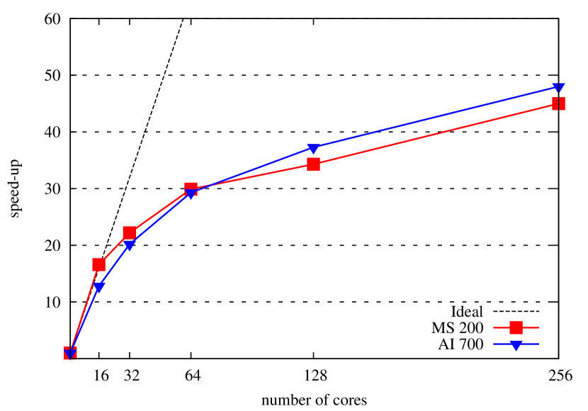
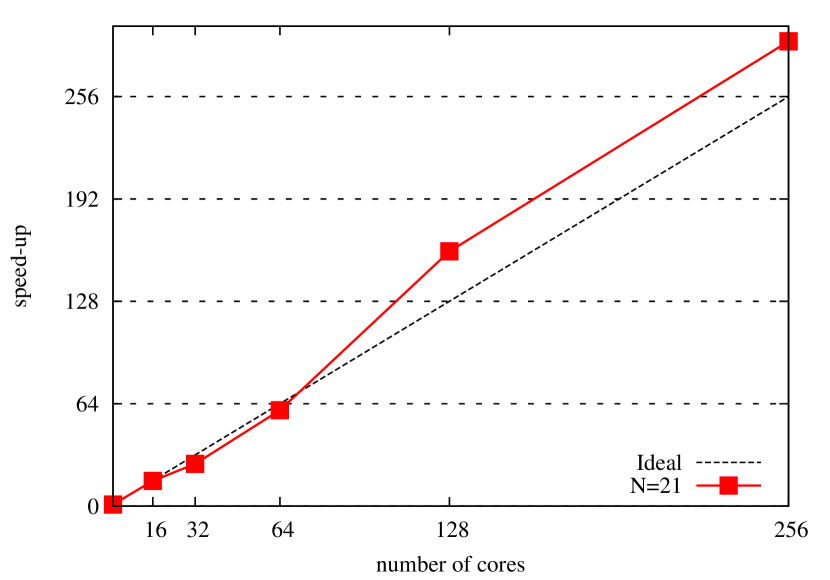
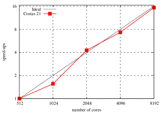
For the two CSPLib benchmarks, one can observe the stabilization point is not yet obtained for 256 cores, even if speed-ups do not increase as fast as the number of cores, i.e., are getting further away from linear speed-up. This is visually depicted on Figure 6. For the Costas Array Problem, the AS algorithm reaches linear or even supra-linear speed-ups up to 256 cores, as depicted in Figure 7. Actually, it scales linearly far beyond this point, i.e., at least up to 8,192 cores, as reported in Diaz et al. [2012].

Figure 6: Speed-ups for CSPLib benchmarks

Figure 7: Speed-ups for the Costas Array Problem

6 Prediction of Parallel Speed-ups

On each problem, the sequential benchmark gives observations of the distribution of the algorithm runtime $f_{Y}$. Yet, the exact distribution is still unknown. It can be any real distribution, not even a classical one. In the following, we will rely on the assumption that $Y$ is distributed with a known parametric distribution. We perform a statistical test, called Kolmogorov-Smirnov test, on the hypothesis $\mathcal{H}_{0}$ that the collected observations correspond to a theoretical distribution. Assuming $\mathcal{H}_{0}$, the test first computes the probability that the distance between the collected data and the theoretical distribution, does not significantly differ from its theoretical value. This probability is called the p-value. Then, the p-value is compared to a fixed threshhold (usually $0.05$). If it is smaller, one rejects $\mathcal{H}_{0}$. For us, it means that the observations do not correspond to the theoretical distribution. If the p-value is high, we will consider that the distribution of $Y$ is approximated by the theoretical one. Note that the Kolmogorov-Smirnov test is a statistical test, which in no way proves that $Y$ follows the distribution. However, it measures how well the observations fit a theoretical curve and, as it will be seen in the following, it is accurate enough for our purpose.

The distributions tested for local search algorithms are the exponential distribution, as suggested by Eadie [1971] , and the lognormal distribution, because it appears to fit the Magic-Square problem. We have also performed the Kolmogorov-Smirnov test on other distributions (e.g. gaussian and Lévy), but obtained negative results w.r.t. the experimental benchmarks, thus we do not include them in the sequel. For each problem, we will need to estimate the value of the parameters of the distribution, which is done on a case by case basis.

Once we have an estimated distribution for the runtimes of $Y$, it becomes possible to compute the expectation of the parallel runtimes and the speed-up thanks to formulas of Section 3.2. All the mathematical calculations are done with Mathematica, a commercial software for symbolic computation Wolfram [2003].

In the following, all the analyses are done on the number of iterations, because they are more likely to be unbiased.

6.1 The All-Interval Series Problem

The analysis is done on $720$ runs of the Adaptive Search algorithm on the instance of All-Interval series for $700$ notes. The sequence of observations is written AI 700 in the following.

We test the hypothesis that the observations admit a shifted exponential distribution as introduced in Section 3.3. The first step consists in estimating the parameter of the distribution, which for a shifted exponential are the value of the shift $x_{0}$ and $\lambda$. We take for $x_{0}$ the minimum observed value, $x_{0}=1217$. The exponential parameter is estimated thanks to the following relation: for a non-shifted exponential distribution, the expectation is $1/\lambda$. Thus we take $\lambda=1/(\text{mean}(\text{AI~{}700})-x_{0})$, which gives $\lambda=9.15956*10^{-6}$.

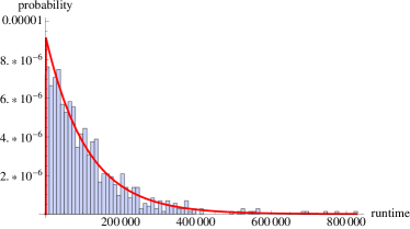
We then run the Kolmogorov-Smirnov test on the shifted exponential distribution with these values of $x_{0}$ and $\lambda$, which answers positively (computed p-value: $0.77435$). We thus admit the hypothesis that AI 700 fits this shifted exponential distribution. As an illustration, Figure 8 shows the normalized histogram of the observed runtimes and the theoretical distribution.

Figure 8: Histogram of the observed number of iterations for $720$ runs on the All-Interval series problem with $N=700$, in blue. In red, the corresponding shifted exponential distribution, statistically estimated.

It is then possible to symbolically compute the speed-up that can be expected with the parallel scheme described in Section 2.2. We use the formulas of Section 3.3 with the estimated parameters and obtain a theoretical expression for the speed-up. This allows us to calculate its value for different number of cores.

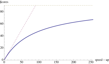
The results are given on Figure 9. With this approximated distribution, the limit of the speed-up when the number of cores tends to infinity is $90.7087$. One can see that, with a 256 cores, the curve has not reached its limit, but comes close. Thus, the speed-up for this instance of All-Interval appears significantly less than linear (linear meaning: equal to the number of cores).

Figure 9: Predicted speed-up for AI 700 as a function of the number of cores (plain blue), with its limit (dashed yellow) and the ideal linear speed-up (dashed pink).

6.2 The Magic-Square Series Problem

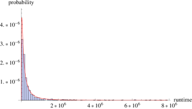
For the Magic-Square problem with $N=200$, the observations are the number of iterations on $662$ runs, with a minimum of $x_{0}=6210$. The Kolmogorov-Smirnov test on a shifted exponential distribution fails, but we obtain a positive result with a lognormal distribution, with $\mu=12.0275$ and $\sigma=1.3398$, shifted to $x_{0}$. These parameters have been estimated with the use of the Mathematica software. As an illustration, Figure 10 shows the observations and the theoretical estimated distribution.

Figure 10: Histogram of the observed number of iterations for $662$ runs on the Magic-Square problem with $N=200$, in blue. In red, the corresponding shifted lognormal distribution, statistically estimated.

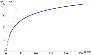
The speed-up can be computed by integrating the minimum distribution with numerical integration techniques. The results are presented on Figure 11. We can observe that the speed-up grows very fast at the origin, which can be explained by the high peak of the lognormal distribution with these parameters. Again, the speed-up is computed with a numerical integration step, and we only draw the curve for integer values of $n$. In this case again, the speed-up is significantly less than linear from 50 cores onwards, and the limit of the speed-up when the number of cores tends to infinity is about 71.5.

Figure 11: Predicted speed-up for MS 200 as a function of the numbers of cores (blue dots), with the ideal linear speed-up (dashed pink).

6.3 The Costas Array Problem

The same analysis is done for the runs of the AS algorithm on the Costas Array problem with $N=21$. The observations are taken from the benchmark with $638$ runs. The sequence of observations is written Costas 21.

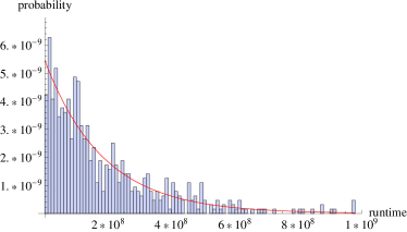
This benchmark has an interesting property: the observed minimum, $3.2*10^{5}$ is neglictible compared to its mean ($1.8*10^{8}$). Thus, we estimate $x_{0}=0$ and perform a Kolmogorov-Smirnov test for a (non-shifted) exponential distribution, with $\lambda=1/\text{mean}(Costas~{}21)=5.4*10^{-9}$. The test is positive for this exponential distribution, with a p-value of $0.751915$. Figure 12 shows the estimated distribution compared to the observations.

Figure 12: Histogram of the observed number of iterations for $638$ runs on the Costas Array problem with $N=21$, in blue. In red, the corresponding shifted exponential distribution, statistically estimated.

The computation of the theoretical speed-up is also done in the same way as for AI 700. Yet, in this case, the observed minimum for $x_{0}$ is so small that we can approximate the observations with a non-shifted distribution, thus the predicted speed-up is strictly linear, as shown in Section 3.3. The results are given on Figure 13. This explains that one may observe linear speed-up when parallelizing Costas Array.

Figure 13: Predicted speed-up for Costas 21 as a function of the number of cores.

7 Analysis

Table 5 presents the comparison between the predicted and the experimental speedups. We can see that the accuracy of the prediction is very good up to 64 parallel cores and then the divergence is limited even for 256 parallel cores.

For the MS 200 problem, the experimental speed-up and the predicted one are almost identical up to 128 cores and diverging by 10% for 256 cores. For the AI 700 problem, the experimental speed-up is less good than the predicted one by a maximum of 30% for 128 and 256 cores. For the Costas 21 problem, the experimental speed-up is better than the predicted one by 15% for 128 and 256 cores.

Problem		speed-up on $k$ cores
		16	32	64	128	256
MS 200	experimental	16.6	22.2	29.9	34.3	45.0
	predicted	15.94	22.04	28.28	34.26	39.7
AI 700	experimental	12.8	20.2	29.3	37.3	48.0
	predicted	13.7	23.8	37.8	53.3	67.2
Costas 21	experimental	15.8	26.4	60.0	159.2	290.5
	predicted	16.0	32.0	64.0	128.0	256.0

Table 5: Comparison: experimental and predicted speedups

It is worth noticing that our model approximates the behaviors of experimental results very closely, as shown by the predicted speed-ups matching closely the real ones. Moreover we can see that on the three benchmark programs, we needed to use three different types of distribution (exponential, shifted exponential and lognormal), in order to approximate the experimental data most closely. This shows that our model is quite general and can accommodate different types of parallel behaviors.

A quite interesting behavior is exhibited by the Costas 21 problem. Our model predicts a linear speedup, up to 10,000 cores and beyond, and the experimental data gathered for this paper confirms this linear speed-up up to 256 cores. Would it scale up with a larger number of cores? Indeed such an experiment has been done up to 8,192 cores on the JUGENE IBM Bluegene/P at the Jülich Supercomputing Center in Germany (with a total 294,912 cores), and reported in Diaz et al. [2012], of which Figure 14 is adapted. We can see that the speed-up is indeed linear up to 8,192 cores, thus showing the adequation of the prediction model with the real data.

Figure 14: Speed-ups for Costas 21 up to 8,192 cores

Finally, let us note that our method exhibits an interesting phenomenon. For the three problems considered, the probability of returning a solution in no iterations is non-null: since they start by a uniform random draw on the search space, there is a very small, but not null, probability that this random initialization directly returns the solution. Hence, in theory, $x_{0}=0$ and the speed-up should be linear, with an infinite limit when the number of cores tends to infinity. Intuitively, if the number of cores tends to infinity, at some point it will be large compared to the size of the search space and one of the cores is likely to immediately find the solution.

Yet, in practice, observations shows that the experimental curves may be better approximated by a shifted exponential with $x_{0}>0$, as it is the case for AI 700. With an exponential distribution, this leads to non-linear speed-up with a finite limit. Indeed, the experimental speed-up for AI 700 is far from linear. On the contrary, Costas 21 has a linear speed-up due to its $x_{0}<<1/\lambda$, which makes the statistical test succeed for $x_{0}\simeq 0$. Firstly, this suggests that the comparison between $x_{0}$ and $1/\lambda$ on a number of observations is a key element for the parallel behavior. It also means that the number of observations needed to properly approximate the sequential distribution probably depends on the problem.

8 Conclusion

We have proposed a theoretical model for predicting and analyzing the speed-ups of Las Vegas algorithms. It is worth noticing that our model mimics the behaviors of the experimental results very closely, as shown by the predicted speedups matching closely the real ones. Our practical experiments consisted in testing the accuracy of the model with respect to three instances of a local search algorithm for combinatorial optimization problems. We showed that the parallel speed-ups predicted by our statistical model are accurate, matching the actual speed-ups very well up to 64 parallel cores and then with a deviation of about 10%, 15% or 30% (depending on the benchmark problem) up to 256 cores.

However, one limitation of our approach is that, in practice, we need to be able to compute the expectation of the minimum distribution. Nevertheless, apart from the exponential distribution for which this computation is easy, recent results in the field of order statistics gives explicit formulas for a number of useful distributions: gaussian, lognormal, gamma, beta. This provides a wide range of tools to analyze different behaviors. In this paper we validated our approach on classical combinatorial optimization and CSP benchmarks, but further research will consider a larger class of problems and algorithms, such as SAT solvers and other randomized algorithms (e.g. quick sort).

Another interesting extension of this work would be to devise a method for predicting the speed-up from scratch, that is, without any knowledge on the algorithm distribution. Preliminary observation suggests that, given a problem and an algorithm, the general shape of the distribution is the same when the size of the instances varies. For example, the different instances of All-Interval that we tested all admit a shifted exponential distribution. If this property is valid on a wide range of problems/algorithms, then we can develop a method for predicting the speed-up for large instances by learning the distribution shape on small instances (which are easier to solve), and then estimating the parallel speed-up for larger instances with our model.

References

- Aarts and Lenstra [1997] E. Aarts and J. K. Lenstra, editors. Local Search in Combinatorial Optimization. John Wiley and Sons, Chichester, UK, 1997.
- Aiex et al. [2007] R. Aiex, M. Resende, and C. Ribeiro. TTT plots: a perl program to create time-to-target plots. Optimization Letters, 1:355–366, 2007. ISSN 1862-4472.
- Aiex et al. [2002] R. M. Aiex, M. G. C. Resende, and C. C. Ribeiro. Probability distribution of solution time in grasp: An experimental investigation. Journal of Heuristics, 8(3):343–373, 2002.
- Alba [2004] E. Alba. Special issue on new advances on parallel meta-heuristics for complex problems. Journal of Heuristics, 10(3):239–380, 2004.
- Babai [1979] L. Babai. Monte-carlo algorithms in graph isomorphism testing. Research Report D.M.S. No. 79-10, Université de Montréal, 1979.
- Beard et al. [2007] J. Beard, J. Russo, K. Erickson, M. Monteleone, and M. Wright. Costas array generation and search methodology. Aerospace and Electronic Systems, IEEE Transactions on, 43(2):522 –538, april 2007. ISSN 0018-9251. 10.1109/TAES.2007.4285351.
- Bessiere [2006] C. Bessiere. Constraint propagation. In F. Rossi, P. van Beek, and T. Walsh, editors, Handbook of Constraint Programming, pages 29–83. Elsevier, 2006.
- Bolze and al. [2006] R. Bolze and al. Grid’5000: A large scale and highly reconfigurable experimental grid testbed. Int. J. High Perform. Comput. Appl., 20(4):481–494, 2006.
- Caniou et al. [2012] Y. Caniou, D. Diaz, F. Richoux, P. Codognet, and S. Abreu. Performance analysis of parallel constraint-based local search. In PPoPP 2012, 17th ACM SIGPLAN Symposium on Principles and Practice of Parallel Programming, New Orleans, LA, USA, 2012. ACM Press. poster paper.
- Codognet and Diaz [2001] P. Codognet and D. Diaz. Yet another local search method for constraint solving. In proceedings of SAGA’01, pages 73–90. Springer Verlag, 2001.
- Codognet and Diaz [2003] P. Codognet and D. Diaz. An efficient library for solving CSP with local search. In T. Ibaraki, editor, MIC’03, 5th International Conference on Metaheuristics, 2003.
- Costas [1984] J. Costas. A study of detection waveforms having nearly ideal range-doppler ambiguity properties. Proceedings of the IEEE, 72(8):996–1009, 1984.
- Crainic and Toulouse [2002] T. Crainic and M. Toulouse. Special issue on parallel meta-heuristics. Journal of Heuristics, 8(3):247–388, 2002.
- Crainic et al. [2004] T. G. Crainic, M. Gendreau, P. Hansen, and N. Mladenovic. Cooperative parallel variable neighborhood search for the -median. Journal of Heuristics, 10(3):293–314, 2004.
- David and Nagaraja [2003] H. David and H. Nagaraja. Order Statistics. Wiley series in probability and mathematical statistics. Probability and mathematical statistics. John Wiley, 2003. ISBN 9780471389262.
- Diaz et al. [2012] D. Diaz, F. Richoux, Y. Caniou, P. Codognet, and S. Abreu. Parallel local search for the costas array problem. In IEEE Workshop on new trends in Parallel Computing and Optimization (PC012), in conjunction with IPDPS 2012, Shanghai, China, May 2012. IEEE Press.
- Drakakis [2006] K. Drakakis. A review of costas arrays. Journal of Applied Mathematics, 2006:1–32, 2006.
- Drakakis et al. [2011a] K. Drakakis, F. Iorio, and S. Rickard. The enumeration of costas arrays of order 28 and its consequences. Advances in Mathematics of Communications, 5(1):69–86, 2011a.
- Drakakis et al. [2011b] K. Drakakis, F. Iorio, S. Rickard, and J. Walsh. Results of the enumeration of costas arrays of order 29. Advances in Mathematics of Communications, 5(3):547–553, 2011b.
- Eadie [1971] W. Eadie. Statistical methods in experimental physics. North-Holland Pub. Co., 1971.
- Galinier and Hao [2000] P. Galinier and J.-K. Hao. A general approach for constraint solving by local search. In 2nd workshop CP-AI-OR’00, Paderborn, Germany, 2000.
- Gent and Walsh [1999] I. P. Gent and T. Walsh. CSPLIB: A benchmark library for constraints. In proceedings of CP’99, pages 480–481. Springer Verlag, 1999.
- Golomb [1984] S. Golomb. Algebraic constructions for Costas arrays. Journal Of Combinatorial Theory Series A, 37(1):13–21, 1984.
- Golomb and Taylor [1984] S. Golomb and H. Taylor. Constructions and properties of Costas arrays. Proceedings of the IEEE, 72(9):1143–1163, 1984.
- Gomes and Selman [2001] C. P. Gomes and B. Selman. Algorithm portfolios. Artificial Intelligence, 126(1-2):43–62, 2001.
- Gonzalez [2007] T. Gonzalez, editor. Handbook of Approximation Algorithms and Metaheuristics. Chapman and Hall / CRC, 2007.
- Hentenryck [1989] P. V. Hentenryck. Constraint Satisfaction in Logic Programming. The MIT Press, 1989.
- Hentenryck and Michel [2005] P. V. Hentenryck and L. Michel. Constraint-Based Local Search. The MIT Press, 2005.
- Hoos and Stütze [2005] H. Hoos and T. Stütze. Stochastic Local Search: Foundations and Applications. Morgan Kaufmann, 2005.
- Ibaraki et al. [2005] T. Ibaraki, K. Nonobe, and M. Yagiura, editors. Metaheuristics: Progress as Real Problem Solvers. Springer Verlag, 2005.
- Lin [1965] S. Lin. Computer solutions of the traveling salesman problem. Bell System Technical Journal, 44:2245–2269, 1965.
- Minton et al. [1992] S. Minton, M. D. Johnston, A. B. Philips, and P. Laird. Minimizing conflicts: A heuristic repair method for constraint satisfaction and scheduling problems. Artificial Intelligence, 58(1-3):161–205, 1992.
- Nadarajah [2008] S. Nadarajah. Explicit expressions for moments of order statistics. Statistics & Probability Letters, 78(2):196–205, Feb. 2008.
- Pardalos et al. [1995] P. M. Pardalos, L. S. Pitsoulis, T. D. Mavridou, and M. G. C. Resende. Parallel search for combinatorial optimization: Genetic algorithms, simulated annealing, tabu search and GRASP. In proceedings of IRREGULAR, pages 317–331, 1995.
- Russo et al. [2010] J. C. Russo, K. G. Erickson, and J. K. Beard. Costas array search technique that maximizes backtrack and symmetry exploitation. In CISS, pages 1–8, 2010.
- Truchet [2004] C. Truchet. Constraints, Local Search and Computer-Aided Music Composition. PhD thesis, University of Paris 7, 2004.
- Truchet and Codognet [2004] C. Truchet and P. Codognet. Musical constraint satisfaction problems solved with adaptive search. Soft Comput., 8(9):633–640, 2004.
- Van Luong et al. [2010] T. Van Luong, N. Melab, and E.-G. Talbi. Local search algorithms on graphics processing units. In Evolutionary Computation in Combinatorial Optimization, pages 264–275. LNCS 6022, Springer Verlag, 2010.
- Verhoeven and Aarts [1995] M. Verhoeven and E. Aarts. Parallel local search. Journal of Heuristics, 1(1):43–65, 1995.
- Wolfram [2003] S. Wolfram. The Mathematica Book, 5th edition. Wolfram Media, 2003. URL http://reference.wolfram.com.