Uncertainty and certainty relations for complementary qubit observables in terms of Tsallis’ entropies

Abstract

Uncertainty relations for more than two observables have found use in quantum information, though commonly known relations pertain to a pair of observables. We present novel uncertainty and certainty relations of state-independent form for the three Pauli observables with use of the Tsallis $\alpha$-entropies. For all real $\alpha\in(0;1]$ and integer $\alpha\geq 2$, lower bounds on the sum of three $\alpha$-entropies are obtained. These bounds are tight in the sense that they are always reached with certain pure states. The necessary and sufficient condition for equality is that the qubit state is an eigenstate of one of the Pauli observables. Using concavity with respect to the parameter $\alpha$, we derive approximate lower bounds for non-integer $\alpha\in(1;+\infty)$. In the case of pure states, the developed method also allows to obtain upper bounds on the entropic sum for real $\alpha\in(0;1]$ and integer $\alpha\geq 2$. For applied purposes, entropic bounds are often used with averaging over the individual entropies. Combining the obtained bounds leads to a band, in which the rescaled average $\alpha$-entropy ranges in the pure-state case. A width of this band is essentially dependent on $\alpha$. It can be interpreted as an evidence for sensitivity in quantifying the complementarity.

I Introduction

The quantum-mechanical concept of complementarity is naturally posed by means of uncertainty relations. Since original Heisenberg’s result heisenberg had been given, numerous ways to pose the uncertainty principle were proposed hall99 ; lahti . Historically, uncertainty relations were focused on pairs of canonically conjugate variables. Today, uncertainty relations attract an attention also due to potential applications in quantum information processing dmg07 ; renes09 ; vsw09 . Entropic functions provide a flexible tool for expressing an uncertainty in quantum measurements. In view of the existing reviews ww10 ; brud11 , we mention here only selected developments. The most traditional form of uncertainty relations was proposed by Robertson robert . Deutsch has discussed advantages of the entropic approach deutsch . For the case of two measurements, the inequality of Maassen and Uffink maass is widely used. This advance has been inspired by the previous conjecture of Kraus kraus87 . It is based on a deep mathematical result known as Riesz’s theorem. In this way, the Maassen–Uffink relation can be extended to a pair of POVM measurements krpr02 ; rast102 .

Entropic inequalities of the Maassen–Uffink type have emphasized a role of mutual unbiasedness. In this regard, we can ask for the entropic uncertainty tradeoff between more than two observables ww10 ; aamb10 . Entropic uncertainty bounds for several observables are also of interest in studying the security of quantum cryptographic protocols dmg07 ; ngbw12 . Uncertainties are mainly quantified by means of the Shannon entropy. An entropic uncertainty relation for $(d+1)$ mutually unbiased bases in $d$-dimensional Hilbert space was obtained ivan92 ; jsan93 and improved jsan95 . The case of arbitrary number of mutually unbiased bases was examined in molm09 . The writer of jsan93 also gave the exact bounds for the qubit case $d=2$. In ww08 , uncertainty relations for a set of anti-commuting observables were given in terms of the Shannon entropy and the so-called collision one (Rényi’s entropy of order 2). Although the Shannon entropy is of great importance, both the Rényi renyi61 and Tsallis tsallis entropies have found use in many issues.

For the traditional case of canonically conjugate observables, the formulation in terms of Rényi’s entropies was given in birula3 . Both the Rényi and Tsallis entropies have been used in expressing the uncertainty principle for trace-preserving super-operators rast104 and the number and annihilation operators rast105 . Reformulations of the entropic uncertainty principle in the presence of quantum memory are considered in BCCRR10 ; clz11 ; fan12 . For quasi-Hermitian models, uncertainty relations have been derived in terms of the so-called unified entropies rastnnh . The Rényi and Tsallis entropies are both included in the family of unified entropies proposed in hey06 . In the papers lars90 ; diaz , the complementarity issue is examined with the sum of squares of probabilities. This sum is closely related to Tsallis’ $2$-entropy. Basing on the Riesz theorem, unified-entropy uncertainty relations for various pairs of measurement have been obtained in rast12qic . In rastijtp , we considered entropic inequalities beyond the scope of Riesz’s theorem. For some pairs of measurements, uncertainty relations were posed in terms of both the Rényi and Tsalis $1/2$-entropies rastijtp .

In the present work, we consider lower and upper bounds on the sum of Tsallis’ $\alpha$-entropies, which quantify uncertainties in measurement of complementary qubit observables. These observables are commonly represented by the Pauli matrices. Results of such a kind may be useful in studying the security of six-state protocols of quantum key distribution. From this viewpoint, some uncertainty relations in information-theoretical terms are extensively treated in dmg07 ; ngbw12 ; bfw11 . The paper is organized as follows. The preliminary material is given in Sect. II. In Sect. III, tight lower bounds on the sum of three entropies of degree $\alpha\in(0;1]$ are obtained. The conditions for equality are considered as well. Tight lower bounds on the entropic sum for integer $\alpha\geq 2$ are derived in Sect. IV. Using concavity with respect to the parameter $\alpha$, we also obtain approximate lower bounds for non-integer $\alpha\in(1;+\infty)$. In Sect. V, we examine upper bounds on the sum of three $\alpha$-entropies in the case of pure states. Here, the bounds are given for all real $\alpha\in(0;1]$ and integer $\alpha\geq 2$. In Sect. VI, we conclude the paper with a summary of results.

II Definition and notation

In this section, the preliminary material is given. In the considered approach, uncertainties of quantum measurements are quantified by means of entropies. In the following, we use the Tsallis entropy. Let $p=\{p_{j}\}$ be a probability distribution supported on $n$ points. For real $\alpha>0\neq 1$, the non-extensive $\alpha$-entropy is defined by tsallis

$$H_{\alpha}(p):=\frac{1}{1-\alpha}{\,}\left(\sum\nolimits_{j=1}^{n}p_{j}^{\alpha}-1\right)=\sum\nolimits_{j=1}^{n}h_{\alpha}(p_{j})\ .$$ (1)

For brevity, we introduce here the function

$$h_{\alpha}(u):=\frac{u^{\alpha}-u}{1-\alpha}=-u^{\alpha}\ln_{\alpha}(u)\ ,$$ (2)

and the $\alpha$-logarithm $\ln_{\alpha}(u):=\bigl{(}u^{1-\alpha}-1\bigr{)}/(1-\alpha)$. When $\alpha\to 1$, we obtain the usual logarithm $\ln{u}$ and the Shannon entropy

$$H_{1}(p)=\sum\nolimits_{j=1}^{n}h_{1}(p_{j})=-\sum\nolimits_{j=1}^{n}p_{j}\ln{p}_{j}\ .$$ (3)

With the factor $\left(2^{1-\alpha}-1\right)^{-1}$ instead of $(1-\alpha)^{-1}$, the entropic function (1) was derived from several axioms by Havrda and Charvát HC67 . In the context of statistical physics, the entropy (1) was developed by Tsallis tsallis .

The $\alpha$-entropy (1) is a concave function of probability distribution. Namely, for all $\lambda\in[0;1]$ and two probability distributions $p=\{p_{j}\}$ and $q=\{q_{j}\}$, we have

$$H_{\alpha}\bigl{(}\lambda{p}+(1-\lambda)q\bigr{)}\geq\lambda{\,}H_{\alpha}(p)+(1-\lambda)H_{\alpha}(q)\ .$$ (4)

This follows from concavity of the function (2) with respect to the variable $u$. Combining this property with $h_{\alpha}(0)=h_{\alpha}(1)=0$, we also get $h_{\alpha}(u)\geq 0$. Tsallis’ $\alpha$-entropy (1) satisfies

$$0\leq{H}_{\alpha}(p)\leq\ln_{\alpha}(n)\ .$$ (5)

The maximum $\ln_{\alpha}(n)$ is reached with the equiprobable distribution, i.e. $p_{j}=1/n$ for all $1\leq{j}\leq{n}$. The minimal zero value is reached with any deterministic distribution, when one of probabilities is 1 and other are all zeros. In fact, the values $u=0$ and $u=1$ are only ones, for which the function $h_{\alpha}(u)$ vanishes. This is actually a manifestation of the fact that the function is strictly concave. Indeed, for $u>0$ we have the relation $h_{\alpha}^{\prime\prime}(u)=-\alpha{u}^{\alpha-2}<0$ sufficient for strict concavity. Following the paper rastijtp , we also put the quantity

$$\Phi_{\alpha}(p):=\sum\nolimits_{j}p_{j}^{\alpha}\ .$$ (6)

As $p_{j}\leq 1$, we have $\Phi_{\alpha}(p)\geq\Phi_{\beta}(p)$ whenever $\alpha<\beta$. With respect to the distribution $p=\{p_{j}\}$, the functional (6) is concave for $\alpha\in(0;1)$ and convex for $\alpha\in(1;+\infty)$. Using this functional, we represent the entropy (1) as

$$H_{\alpha}(p)=\frac{\Phi_{\alpha}(p)-1}{1-\alpha}\ .$$ (7)

Rényi entropies form another especially important family of one-parametric extensions of the Shannon entropy. Basic properties of this extension are examined in the original work renyi61 . Some of applications of the Rényi and Tsallis entropies in quantum information theory are discussed in bengtsson .

In the present paper, we will deal with the qubit case $n=2$. In this case, three complementary observables are usually represented by the Pauli matrices $\boldsymbol{\sigma}_{x}$, $\boldsymbol{\sigma}_{y}$, $\boldsymbol{\sigma}_{z}$, namely

$$\boldsymbol{\sigma}_{x}=\begin{pmatrix}0&1\\ 1&0\end{pmatrix}\ ,\qquad\boldsymbol{\sigma}_{y}=\begin{pmatrix}0&-i\\ i&0\end{pmatrix}\ ,\qquad\boldsymbol{\sigma}_{z}=\begin{pmatrix}1&0\\ 0&-1\end{pmatrix}\ .$$ (8)

Historically, these matrices were introduced in describing spin-$1/2$ observables. Each of the matrices has the eigenvalues $\pm 1$. Let $\bigl{\{}|0\rangle,|1\rangle\bigr{\}}$ denote the eigenbasis of $\boldsymbol{\sigma}_{z}$, in the matrix form

$$|0\rangle=\begin{pmatrix}1\\ 0\end{pmatrix}\ ,\qquad|1\rangle=\begin{pmatrix}0\\ 1\end{pmatrix}\ .$$ (9)

The normalized eigenvectors of $\boldsymbol{\sigma}_{x}$ and $\boldsymbol{\sigma}_{y}$ can be written as

$$|x_{\pm}\rangle=\frac{1}{\sqrt{2}}\begin{pmatrix}1\\ \pm 1\end{pmatrix}\ ,\qquad|y_{\pm}\rangle=\frac{1}{\sqrt{2}}\begin{pmatrix}1\\ \pm{i}\end{pmatrix}\ .$$ (10)

We obviously have $\boldsymbol{\sigma}_{x}|x_{\pm}\rangle=\pm|x_{\pm}\rangle$ and $\boldsymbol{\sigma}_{y}|y_{\pm}\rangle=\pm|y_{\pm}\rangle$. Note that the kets $|y_{+}\rangle$ and $|y_{-}\rangle$ correspond to the states of right and left circular polarizations, respectively. The three bases given by (9) and (10) are mutually unbiased. Measurements in these eigenbases are used in six-state cryptographic protocols ngbw12 ; bfw11 .

Let us write the probabilities corresponding to measurement of each of the observables $\boldsymbol{\sigma}_{x}$, $\boldsymbol{\sigma}_{y}$, $\boldsymbol{\sigma}_{z}$. Up to a unimodular factor, we can express a normalized pure state as

$$|\psi\rangle=\cos\tau|0\rangle+e^{i\varphi}\sin\tau|1\rangle=\begin{pmatrix}\cos\tau\\ e^{i\varphi}\sin\tau\end{pmatrix}\ ,$$ (11)

where $\tau$ and $\varphi$ are real numbers. Assuming $\varphi\in[0;2\pi)$, we will take $\tau\in[0;\pi/2]$, since the reversed sign in the state vector has no physical relevance. The probabilities are calculated as follows. With respect to the basis $\bigl{\{}|x_{+}\rangle,|x_{-}\rangle\bigr{\}}$, we obtain

$$p_{\pm}=\bigl{|}\langle{x}_{\pm}|\psi\rangle\bigr{|}^{2}=\frac{1\pm\sin 2\tau\cos\varphi}{2}\ .$$ (12)

With respect to the basis $\bigl{\{}|y_{+}\rangle,|y_{-}\rangle\bigr{\}}$, we further have

$$q_{\pm}=\bigl{|}\langle{y}_{\pm}|\psi\rangle\bigr{|}^{2}=\frac{1\pm\sin 2\tau\sin\varphi}{2}\ .$$ (13)

With respect to the basis $\bigl{\{}|0\rangle,|1\rangle\bigr{\}}$, we obtain $r_{+}=\bigl{|}\langle 0|\psi\rangle\bigr{|}^{2}=\cos^{2}\tau$ and $r_{-}=\bigl{|}\langle 1|\psi\rangle\bigr{|}^{2}=\sin^{2}\tau$, or merely

$$r_{\pm}=\frac{1\pm\cos 2\tau}{2}\ .$$ (14)

Substituting the post-measurements distributions (12), (13), (14) into the right-hand side of (1), we respectively obtain the entropies $H_{\alpha}\bigl{(}\boldsymbol{\sigma}_{x}|\psi\bigr{)}$, $H_{\alpha}\bigl{(}\boldsymbol{\sigma}_{y}|\psi\bigr{)}$, $H_{\alpha}\bigl{(}\boldsymbol{\sigma}_{z}|\psi\bigr{)}$ for the state (11). We will derive lower and upper bounds on the sum of such entropies for pure states and, by concavity, for mixed ones.

III Tight lower bounds on the sum of entropies of degree $\alpha\in(0;1]$

In this section, we derive tight lower bounds on the entropic sum for $\alpha\in(0;1]$. A desired bound will firstly be obtained for pure states of the form (11), when the probabilities are given by (12), (13) and (14). Using the concavity properties, we then extend the result to mixed states of a qubit. For $\alpha>0\neq 1$, we introduce the function

$$F_{\alpha}(\tau,\varphi)=\frac{1}{1-\alpha}{\,}\left(\sum\nolimits_{j=\pm}\left(p_{j}^{\alpha}+q_{j}^{\alpha}+r_{j}^{\alpha}\right)-3\right)\ .$$ (15)

This function represents the entropic sum $H_{\alpha}\bigl{(}\boldsymbol{\sigma}_{x}|\psi\bigr{)}+H_{\alpha}\bigl{(}\boldsymbol{\sigma}_{y}|\psi\bigr{)}+H_{\alpha}\bigl{(}\boldsymbol{\sigma}_{z}|\psi\bigr{)}$ in terms of the variables $\tau$ and $\varphi$. Formally, we aim to minimize (15) in the domain of interest. As was noted above, the variables are initially in the intervals $\tau\in[0;\pi/2]$ and $\varphi\in[0;2\pi)$. In the task of optimization, however, we can restrict a consideration to the rectangular domain

$$D:=\bigl{\{}(\tau,\varphi):{\>}\tau\in[0;\pi/4],{\>}\varphi\in[0;\pi/4]\bigr{\}}\ .$$ (16)

In the total domain $\bigl{\{}(\tau,\varphi):{\>}\tau\in[0;\pi/2],{\>}\varphi\in[0;2\pi)\bigr{\}}$, the function $F_{\alpha}(\tau,\varphi)$ takes the same range of values as on the domain (16). The justification is as follows. First, mapping $\varphi\mapsto\varphi-\pi$ merely swaps two values in the pairs (12) and (13). For each of the pair $p_{\pm}$ and $q_{\pm}$, therefore, the interval $\varphi\in[\pi;2\pi]$ leads to the same values as the interval $\varphi\in[0;\pi]$. Further, under mapping $\varphi\mapsto\pi-\varphi$ the probabilities $p_{\pm}$ are swapped and the probabilities $q_{\pm}$ are unchanged. Hence, we can restrict a consideration to values of $F_{\alpha}(\tau,\varphi)$ for $\varphi\in[0;\pi/2]$. Acting in this interval, mapping $\varphi\mapsto\pi/2-\varphi$ implies swapping $p_{j}$ and $q_{j}$, where $j=\pm$. So, the interval $\varphi\in[\pi/4;\pi/2]$ does not give new values of the function $F_{\alpha}(\tau,\varphi)$, and we shall now assume $\varphi\in[0;\pi/4]$. Finally, we use mapping $\tau\mapsto\pi/2-\tau$, which does not alter $\sin 2\tau$ and reverses the sign of $\cos 2\tau$. Hence, only the probabilities $r_{\pm}$ are merely swapped. The following statement takes place.

Theorem 1

Let qubit state be described by density matrix $\boldsymbol{\rho}$. For all $\alpha\in(0;1]$, the entropic sum satisfies

$$H_{\alpha}\bigl{(}\boldsymbol{\sigma}_{x}|\boldsymbol{\rho}\bigr{)}+H_{\alpha}\bigl{(}\boldsymbol{\sigma}_{y}|\boldsymbol{\rho}\bigr{)}+H_{\alpha}\bigl{(}\boldsymbol{\sigma}_{z}|\boldsymbol{\rho}\bigr{)}\geq 2\ln_{\alpha}(2)\ ,$$ (17)

with equality if and only if the qubit state is an eigenstate of either of the observables $\boldsymbol{\sigma}_{x}$, $\boldsymbol{\sigma}_{y}$, $\boldsymbol{\sigma}_{z}$.

Proof. We first assume that $\alpha\neq 1$. Let us show that the right-hand side of (17) gives the minimum of (15) in the domain (16). Differentiating with respect to $\varphi$, we obtain

$$\frac{\partial}{\partial\varphi}{\>}F_{\alpha}(\tau,\varphi)=-\frac{\alpha}{2(1-\alpha)}\left(p_{+}^{\alpha-1}-p_{-}^{\alpha-1}\right)\sin 2\tau\sin\varphi$$

$$+\frac{\alpha}{2(1-\alpha)}\left(q_{+}^{\alpha-1}-q_{-}^{\alpha-1}\right)\sin 2\tau\cos\varphi=\alpha 2^{-\alpha}uv\bigl{[}f_{\alpha}(u)-f_{\alpha}(v)\bigr{]}{\>}.$$ (18)

For brevity, we introduce here the variables $u=\sin 2\tau\cos\varphi$, $v=\sin 2\tau\sin\varphi$, and the function

$$f_{\alpha}(u)=\frac{(1-u)^{\alpha-1}-(1+u)^{\alpha-1}}{(1-\alpha)u}\ .$$ (19)

Except for the boundary lines of the rectangle (16), we have $0<v<u<1$. We now claim that the function $f_{\alpha}(u)$ monotonically increases with $u\in(0;1)$ for all real $\alpha\in(0;1)$. This fact easily follows from its expansion as a power series about the origin. Using the binomial theorem, we actually obtain

$$f_{\alpha}(u)=\sum_{k=0}^{\infty}\frac{2}{1-\alpha}{\,}\binom{2k+1-\alpha}{2k+1}u^{2k}\ .$$ (20)

We stress that this series contains only strictly positive coefficients. In fact, for $k\geq 0$ and $\alpha\in(0;1)$ we have

$$\frac{2}{1-\alpha}{\,}\binom{2k+1-\alpha}{2k+1}=2{\>}\frac{(2k+1-\alpha)(2k-\alpha)\cdots(2-\alpha)}{(2k+1)!}>0\ .$$ (21)

So the function (20) monotonically increases with $u\in(0;1)$. Hence, the inequality $v<u$ implies $f_{\alpha}(v)<f_{\alpha}(u)$. In the interior of the domain (16), therefore, the derivative (18) is strictly positive. Here, the function $F_{\alpha}(\tau,\varphi)$ increases with $\varphi$. On the boundary lines $\tau=0$ and $\tau=\pi/4$, we have $\partial{F}_{\alpha}/\partial\varphi=0$. These facts implies that the minimal and maximal values of $F_{\alpha}(\tau,\varphi)$ in the domain (16) are reached on the lines $\varphi=0$ and $\varphi=\pi/4$, respectively. To find the minimum, we substitute $\varphi=0$ and rewrite probabilities as

$$p_{\pm}=\frac{1\pm\sin 2\tau}{2}\ ,\qquad q_{\pm}=\frac{1}{2}\ ,\qquad r_{\pm}=\frac{1\pm\cos 2\tau}{2}\ .$$ (22)

Using these formulas and differentiating with respect to $\tau$, we further obtain

$$\frac{\partial}{\partial\tau}{\>}F_{\alpha}(\tau,0) =\frac{\alpha}{1-\alpha}\left(p_{+}^{\alpha-1}-p_{-}^{\alpha-1}\right)\cos 2\tau-\frac{\alpha}{1-\alpha}\left(r_{+}^{\alpha-1}-r_{-}^{\alpha-1}\right)\sin 2\tau$$

$$=\alpha 2^{1-\alpha}uv\bigl{[}f_{\alpha}(u)-f_{\alpha}(v)\bigr{]}\ ,$$ (23)

where the variables $u=\cos 2\tau$ and $v=\sin 2\tau$. Since $u>v$ for $\tau\in(0;\pi/8)$ and $u<v$ for $\tau\in(\pi/8;\pi/4)$, the derivative (23) is strictly positive in the former interval and strictly negative in the latter one. So, the minimal value of $F_{\alpha}(\tau,0)$ is reached at the end points of the interval $\tau\in[0;\pi/4]$. In both the points, the function (15) is equal to the right-hand side of (17). This bound holds for all pure states and remains valid for mixed states due to concavity of the entropy (1).

Let us proceed to conditions for equality. In the domain (16), the function $F_{\alpha}(\tau,\varphi)$ takes its minimum $2\ln_{\alpha}(2)$ only at the points $\tau=\varphi=0$ and $\tau=\pi/4$, $\varphi=0$. In both the points, one of the distributions $\{p_{\pm}\}$, $\{q_{\pm}\}$, $\{r_{\pm}\}$ is deterministic and other two are herewith equiprobable. This is the only case, when the minimum of $F_{\alpha}(\tau,\varphi)$ takes place. As it is seen from (22), the distribution $\{q_{\pm}\}$ is inevitably equiprobable for the above two points. The total domain $\bigl{\{}(\tau,\varphi):{\>}\tau\in[0;\pi/2],{\>}\varphi\in[0;2\pi)\bigr{\}}$ for the state (11) contains also points, in which the distribution $\{q_{\pm}\}$ is deterministic. In any case, it is necessary for reaching the minimum that one of the distributions be deterministic. In other words, the state $|\psi\rangle$ should be an eigenstate of one of the observables $\boldsymbol{\sigma}_{x}$, $\boldsymbol{\sigma}_{y}$, $\boldsymbol{\sigma}_{z}$. Of course, this condition is sufficient as well. We shall now prove that the inequality (17) cannot be saturated with impure states. Let the spectral decomposition of impure $\boldsymbol{\rho}$ be written as

$$\boldsymbol{\rho}=\lambda_{+}|\psi_{+}\rangle\langle\psi_{+}|+\lambda_{-}|\psi_{-}\rangle\langle\psi_{-}|\ ,$$ (24)

where eigenstates are mutually orthogonal and strictly positive eigenvalues obey the condition $\lambda_{+}+\lambda_{-}=1$. By concavity of the entropy (1), we write

$$\sum_{\nu=x,y,z}H_{\alpha}\bigl{(}\boldsymbol{\sigma}_{\nu}|\boldsymbol{\rho}\bigr{)}\geq\lambda_{+}\sum_{\nu=x,y,z}H_{\alpha}\bigl{(}\boldsymbol{\sigma}_{\nu}|\psi_{+}\bigr{)}+\lambda_{-}\sum_{\nu=x,y,z}H_{\alpha}\bigl{(}\boldsymbol{\sigma}_{\nu}|\psi_{-}\bigr{)}\ .$$ (25)

If the sum of $\alpha$-entropies of the state $|\psi_{+}\rangle$ or $|\psi_{-}\rangle$ does not reach the lower bound $2\ln_{\alpha}(2)$, the left-hand side of (25) does not reach this bound as well. So, the question is reduced to the case, when the matrix $\boldsymbol{\rho}$ is diagonal with respect to eigenbasis of either of the $\boldsymbol{\sigma}_{x}$, $\boldsymbol{\sigma}_{y}$, $\boldsymbol{\sigma}_{z}$. For definiteness, we assume that the $\boldsymbol{\rho}$ commutes with $\boldsymbol{\sigma}_{x}$ and $|\psi_{\pm}\rangle=|x_{\pm}\rangle$. Measuring any of the $\boldsymbol{\sigma}_{y}$ and $\boldsymbol{\sigma}_{z}$ in the state $\boldsymbol{\rho}$ results in the equiprobable distribution, whence $H_{\alpha}\bigl{(}\boldsymbol{\sigma}_{y}|\boldsymbol{\rho}\bigr{)}=H_{\alpha}\bigl{(}\boldsymbol{\sigma}_{z}|\boldsymbol{\rho}\bigr{)}=\ln_{\alpha}(2)$. Measuring the $\boldsymbol{\sigma}_{x}$ in the state $\boldsymbol{\rho}$, we obtain outcomes $\pm 1$ with probabilities $\lambda_{\pm}$, respectively. Except for the two cases, when $\lambda_{+}=1$ or $\lambda_{-}=1$, this probability distribution is not deterministic and $H_{\alpha}\bigl{(}\boldsymbol{\sigma}_{x}|\boldsymbol{\rho}\bigr{)}>0$. The latter implies that the sum of three entropies is strictly larger than $2\ln_{\alpha}(2)$.

Let us consider the standard case $\alpha=1$. Taking the limit $\alpha\to 1^{-}$ in the inequality (17), we obtain the known lower bound $2\ln 2$ on the standard entropic sum. In this way, however, conditions for equality are still not resolved. Nevertheless, we could repeat the above reasons with the function

$$F_{1}(\tau,\varphi)=\sum_{j=\pm}\left(-p_{j}\ln{p}_{j}-q_{j}\ln{q}_{j}-r_{j}\ln{r}_{j}\right)\ .$$ (26)

A sketch of the derivation is given below. Similarly to (18) and (19), we obtain the formulas

$$\frac{\partial}{\partial\varphi}{\>}F_{1}(\tau,\varphi)=\frac{uv}{2}{\,}\bigl{[}f_{1}(u)-f_{1}(v)\bigr{]}\ ,$$ (27)

$$f_{1}(u)=\frac{1}{u}{\>}\ln\!\left(\frac{1+u}{1-u}\right)=\sum_{k=0}^{\infty}\frac{2}{2k+1}{\>}u^{2k}\ ,$$ (28)

where $u=\sin 2\tau\cos\varphi$, $v=\sin 2\tau\sin\varphi$. The function $f_{1}(u)$ monotonically increases, whence $\partial{F}_{1}(\tau,\varphi)/\partial\varphi>0$ for $0<v<u<1$. Hence, the minimal value of $F_{1}(\tau,\varphi)$ in the domain (16) is reached on the line $\varphi=0$. Differentiating $F_{1}(\tau,0)$ with respect to $\tau$, we also obtain the formula

$$\frac{\partial}{\partial\tau}{\>}F_{1}(\tau,0)=uv\bigl{[}f_{1}(u)-f_{1}(v)\bigr{]}\ ,$$ (29)

in which $u=\cos 2\tau$ and $v=\sin 2\tau$. To sum up, we see that the function $F_{1}(\tau,\varphi)$ takes its minimum $2\ln 2$ only at the points $\tau=\varphi=0$ and $\tau=\pi/4$, $\varphi=0$. As above, this leads to the claimed conditions for equality. $\blacksquare$

Theorem 1 provides a lower bound on the sum of three entropies for all $\alpha\in(0;1]$. This bound is tight in the sense that it is certainly reached with an eigenstate of one of the complementary observables. Previously, the standard case $\alpha=1$ has been studied in jsan93 . In this regard, we have extended the uncertainty relation for three spin-$1/2$ observables to an entire family of $\alpha$-entropic relations for all $\alpha\in(0;1]$. In general, a utility of entropic bounds with a parametric dependence was noted in maass . For example, this dependence allows to find more exactly the domain of acceptable values for unknown probabilities with respect to known ones. For the standard case $\alpha=1$, the writers of clz11 have derived a stronger bound of state-dependent form. In their lower bound, the term $2\ln{2}$ is added by the von Neumann entropy of the $\boldsymbol{\rho}$. It would be of interest to examine this issue with respect to Tsallis-entropy relations.

IV Lower bounds on the sum of entropies of degree $\alpha\in(1;+\infty)$

In this section, we obtain two connected results. The first result provides tight lower bounds on the entropic sum for integer $\alpha\geq 2$. The second result presents approximate lower bounds for non-integer $\alpha\in(1;+\infty)$. To derive the claims, we will use a lemma. Assuming the expressions (12)–(14), we introduce the function

$$G_{\alpha}(\tau,\varphi):=3-\Phi_{\alpha}(p)-\Phi_{\alpha}(q)-\Phi_{\alpha}(r)=3-\sum_{j=\pm}\left(p_{j}^{\alpha}+q_{j}^{\alpha}+r_{j}^{\alpha}\right)\ .$$ (30)

which is closely related to (15). In the present section, the function $G_{\alpha}(\tau,\varphi)$ will be more convenient. With the function (30), we have the following statement.

Lemma 2

For integer $\alpha\geq 1$, the minimal value of the function $G_{\alpha}(\tau,\varphi)$ in the domain (16) is equal to

$$\underset{D}{\min}{\>}G_{\alpha}(\tau,\varphi)=2\left(1-2^{1-\alpha}\right){\>.}$$ (31)

For integer $\alpha\geq 4$, this minimum is reached only at the points $\tau=\varphi=0$ and $\tau=\pi/4$, $\varphi=0$.

Proof. By doing some simple algebra, we obtain $G_{1}(\tau,\varphi)\equiv 0$, $G_{2}(\tau,\varphi)\equiv 1$, and $G_{3}(\tau,\varphi)\equiv 3/2$. These values concur with the formula (31). So, we should prove (31) only for integer $\alpha\geq 4$. Differentiating with respect to $\varphi$, we obtain

$$\frac{\partial}{\partial\varphi}{\>}G_{\alpha}(\tau,\varphi) =\frac{\alpha}{2}\left(p_{+}^{\alpha-1}-p_{-}^{\alpha-1}\right)\sin 2\tau\sin\varphi-\frac{\alpha}{2}\left(q_{+}^{\alpha-1}-q_{-}^{\alpha-1}\right)\sin 2\tau\cos\varphi$$

$$=\alpha 2^{-\alpha}uv\bigl{[}g_{\alpha}(u)-g_{\alpha}(v)\bigr{]}{\>}.$$ (32)

For brevity, the result is expressed in terms of the variables $u=\sin 2\tau\cos\varphi$, $v=\sin 2\tau\sin\varphi$, and the function

$$g_{\alpha}(u)=\frac{(1+u)^{\alpha-1}-(1-u)^{\alpha-1}}{u}\ .$$ (33)

Except for the boundary lines of the rectangle (16), we have $0<v<u<1$. We now claim that the function $g_{\alpha}(u)$ monotonically increases with $u\in(0;1)$ for all integer $\alpha\geq 4$. This fact easily follows from its representation as a polynomial. Using the binomial formula, it is written as

$$g_{\alpha}(u)=\sum_{k=0}^{\lfloor{\alpha/2}\rfloor-1}2\binom{\alpha-1}{2k+1}u^{2k}\ .$$ (34)

By $\lfloor{u}\rfloor$, we will mean the floor of real number $u$. Note that $g_{1}(u)\equiv 0$, $g_{2}(u)\equiv 2$, and $g_{3}(u)\equiv 4$, whence the derivative (32) vanishes for $\alpha=1,2,3$. For $\alpha\geq 4$, the sum (34) is not constant, as non-zero powers are inserted. Further, the coefficients in (34) are all strictly positive, whence we see a monotone increase.

Since the function (33) monotonically increases with $u\in(0;1)$, the inequality $v<u$ implies $g_{\alpha}(v)<g_{\alpha}(u)$. In the interior of the rectangle (16), therefore, the derivative (32) is strictly positive. Here, the function $G_{\alpha}(\tau,\varphi)$ increases with $\varphi$. On the boundary lines $\tau=0$ and $\tau=\pi/4$, we have $u=v$ and zero derivative (32). These two points imply that the minimal and maximal values of $G_{\alpha}(\tau,\varphi)$ in the domain (16) are reached on the boundary lines $\varphi=0$ and $\varphi=\pi/4$, respectively. To find the minimum, we take $\varphi=0$ and write the expressions (22). Differentiating with respect to $\tau$, we further obtain

$$\frac{\partial}{\partial\tau}{\>}G_{\alpha}(\tau,0) =-\alpha\left(p_{+}^{\alpha-1}-p_{-}^{\alpha-1}\right)\cos 2\tau+\alpha\left(r_{+}^{\alpha-1}-r_{-}^{\alpha-1}\right)\sin 2\tau$$

$$=\alpha 2^{1-\alpha}uv\bigl{[}g_{\alpha}(u)-g_{\alpha}(v)\bigr{]}\ ,$$ (35)

where the variables $u=\cos 2\tau$ and $v=\sin 2\tau$. Of course, the term $g_{\alpha}(u)$ is constant and the derivative (35) is zero for $\alpha=1,2,3$. For integer $\alpha\geq 4$, the $g_{\alpha}(u)$ monotonically increases, whence we see the following. As $u>v$ for $\tau\in(0;\pi/8)$ and $u<v$ for $\tau\in(\pi/8;\pi/4)$, the derivative (35) is strictly positive in the former interval and strictly negative in the latter one. So, the minimal value of $G_{\alpha}(\tau,0)$ is reached at the end points of the interval $\tau\in[0;\pi/4]$. In both the points, the function (30) is equal to the right-hand side of (31). $\blacksquare$

Using the statement of Lemma 2, we can obtain a lower bound on the entropic sum for integer $\alpha\geq 2$. The result is posed in the following way.

Theorem 3

Let qubit state be described by density matrix $\boldsymbol{\rho}$. For all integer $\alpha\geq 2$, the entropic sum satisfies

$$H_{\alpha}\bigl{(}\boldsymbol{\sigma}_{x}|\boldsymbol{\rho}\bigr{)}+H_{\alpha}\bigl{(}\boldsymbol{\sigma}_{y}|\boldsymbol{\rho}\bigr{)}+H_{\alpha}\bigl{(}\boldsymbol{\sigma}_{z}|\boldsymbol{\rho}\bigr{)}\geq 2\ln_{\alpha}(2)\ .$$ (36)

For integer $\alpha\geq 4$, equality takes place if and only if the qubit state is an eigenstate of either of the $\boldsymbol{\sigma}_{x}$, $\boldsymbol{\sigma}_{y}$, $\boldsymbol{\sigma}_{z}$.

Proof. Dividing the right-hand side of (31) by $(\alpha-1)$, we get the right-hand side of (36). This bound holds for all pure states and remains valid for mixed states due to concavity of the entropy (1). For $\alpha=2,3$, the inequality (36) is actually saturated with any pure state. The claim follows from the above equalities $G_{2}(\tau,\varphi)\equiv 1$ and $G_{3}(\tau,\varphi)\equiv 3/2$. Remaining task is to prove conditions for equality in the case of integer $\alpha\geq 4$. In general, this task can be resolved similarly to conditions for equality in the relation (17) (see the second part of the proof of Theorem 1). First, we notice that the $G_{\alpha}(\tau,\varphi)$ takes its minimum (31), if and only if one of the distributions $\{p_{\pm}\}$, $\{q_{\pm}\}$, $\{r_{\pm}\}$ is deterministic. Hence, the state $|\psi\rangle$ should be an eigenstate of one of the observables $\boldsymbol{\sigma}_{x}$, $\boldsymbol{\sigma}_{y}$, $\boldsymbol{\sigma}_{z}$. Second, we prove that the inequality (36) cannot be saturated with impure states. We refrain from presenting the details here. $\blacksquare$

As was mentioned above, for $\alpha=2,3$ the inequality (36) is saturated with each pure state. On the other hand, with an impure state the entropic sum can be increased up to the maximum $3\ln_{\alpha}(2)$. This upper bound is explained in the next section. The lower bound of Theorem 3 is tight in the sense that it is always reached with an eigenstate of one of the complementary observables. It holds for all integer $\alpha\geq 2$. Basing on the result (31), we can also obtain an approximate lower bound on the entropic sum for arbitrary $\alpha\in(1;+\infty)$. Here, functional properties of $\Phi_{\alpha}(p)$ with respect to the parameter $\alpha$ are significant. Namely, the quantity $\Phi_{\alpha}(p)$ is a convex function of $\alpha>0$. Calculating the second derivative, one actually gives

$$\frac{\partial^{2}\Phi_{\alpha}(p)}{\partial\alpha^{2}}=\sum\nolimits_{p_{j}\neq 0}p_{j}^{\alpha}\bigl{(}\ln{p}_{j}\bigr{)}^{2}\geq 0\ .$$ (37)

For fixed probabilities, therefore, the quantity (30) is a concave function of $\alpha$. Using this concavity, we formulate the following bound.

Theorem 4

For all real $\alpha\in(1;+\infty)$ and arbitrary qubit density matrix $\boldsymbol{\rho}$, the entropic sum satisfies

$$H_{\alpha}\bigl{(}\boldsymbol{\sigma}_{x}|\boldsymbol{\rho}\bigr{)}+H_{\alpha}\bigl{(}\boldsymbol{\sigma}_{y}|\boldsymbol{\rho}\bigr{)}+H_{\alpha}\bigl{(}\boldsymbol{\sigma}_{z}|\boldsymbol{\rho}\bigr{)}\geq 2{\>}\frac{1-2^{1-\lfloor\alpha\rfloor}}{\alpha-1}+2^{1-\lfloor\alpha\rfloor}{\,}\frac{\alpha-\lfloor\alpha\rfloor}{\alpha-1}\ .$$ (38)

Proof. Suppose that $\alpha\in(n;n+1)$, where integer $n=\lfloor\alpha\rfloor\geq 1$. The principal point is that the term $\Phi_{\alpha}(p)$ is a convex function of the parameter $\alpha$. Therefore, for arbitrary distributions $\{p_{\pm}\}$, $\{q_{\pm}\}$, $\{r_{\pm}\}$ the term (30) is concave with respect to $\alpha$. It follows from the concavity that

$$G_{\alpha}-G_{n}-\left(G_{n+1}-G_{n}\right)(\alpha-n)\geq 0\ ,$$ (39)

for all $\alpha\in[n;n+1]$. Indeed, the left-hand side of (39) is a concave function of $\alpha$ and vanishes in both the end points $\alpha=n$ and $\alpha=n+1$. Combining the inequality (39) with the result (31), we get

$$G_{\alpha}(\tau,\varphi)\geq(n+1-\alpha){\,}G_{n}(\tau,\varphi)+(\alpha-n){\,}G_{n+1}(\tau,\varphi)\geq 2\left(1-2^{1-n}\right)+2^{1-n}(\alpha-n){\,}.$$ (40)

Dividing (40) by $(\alpha-1)$ completes the proof. $\blacksquare$

The statement of Theorem 4 provides a non-trivial lower bound on the sum of three $\alpha$-entropies. By construction, this bound is not exact in general. In the limit $\alpha\to 1^{+}$, the right-hand side of (38) gives $1$, whereas the tight bound is $2\ln 2\approx 1.386$. Nevertheless, the lower bound (38) is tight for all integer $\alpha\geq 2$. In combination, the relations (17) and (38) give lower bounds on the entropic sum for all real $\alpha>0$. So we have obtained uncertainty relations in terms of Tsallis’ $\alpha$-entropies for arbitrary positive values of the parameter. In the case of several observables, entropic bounds are often given with averaging over the individual entropies ww10 ; ngbw12 . It is also convenient to relate each $\alpha$-entropy with the value $\ln_{\alpha}(2)$, which represents the maximum. For all real $\alpha\in(0;1]$ and integer $\alpha\geq 2$, we obtain the tight lower bound on the rescaled average $\alpha$-entropy

$$\frac{1}{3\ln_{\alpha}(2)}\sum_{\nu=x,y,z}H_{\alpha}\bigl{(}\boldsymbol{\sigma}_{\nu}|\boldsymbol{\rho}\bigr{)}\geq\frac{2}{3}\ .$$ (41)

In the left-hand side, the denominator involves $3$ due to averaging over the three observables and $\ln_{\alpha}(2)$ as a natural entropic scale. In the range of its validity, the lower bound (41) does not depend on the parameter $\alpha$. In a similar manner, the relation (38) leads to the average-entropy lower bound, which is dependent on non-integer $\alpha>1$.

V Some tight upper bounds on the entropic sum in the case of pure states

In this section, we study upper bounds on the sum of three $\alpha$-entropies for complementary qubit observables. In general, these bounds are essentially depend on a type of considered states. The completely mixed state is described by density operator $\boldsymbol{\rho}_{*}=\openone/2$, where $\openone$ denotes the identity $2\times 2$-matrix. Measuring each of the observables $\boldsymbol{\sigma}_{x}$, $\boldsymbol{\sigma}_{y}$, $\boldsymbol{\sigma}_{z}$ in this state will lead to the equiprobable distribution. With this distribution, the entropy (1) takes its maximal value $\ln_{\alpha}(2)$. For all $\alpha>0$ and arbitrary density matrix $\boldsymbol{\rho}$, we can then write the upper bound

$$\sum_{\nu=x,y,z}H_{\alpha}\bigl{(}\boldsymbol{\sigma}_{\nu}|\boldsymbol{\rho}\bigr{)}\leq\sum_{\nu=x,y,z}H_{\alpha}\bigl{(}\boldsymbol{\sigma}_{\nu}|\boldsymbol{\rho}_{*}\bigr{)}=3\ln_{\alpha}(2)\ .$$ (42)

Developing the issue, we ask for upper entropic bounds in the case of pure states. In line with the method of previous sections, one will obtain tight bounds from above for real $\alpha\in(0;1]$ and integer $\alpha\geq 2$. Before the derivation, we present some intuitive reasons that make the result physically reasonable. For the pure state (11), the sum of three $\alpha$-entropies is represented by the function (15). Formally, we aim to maximize this function in the domain (16). As we have seen in the proof of Theorem 1, for $\alpha\in(0;1]$ the maximum is reached on the line $\varphi=\pi/4$. The same remains valid for integer $\alpha\geq 2$, though we have dealt with (30) in Lemma 2. Taking $\varphi=\pi/4$ in the formulas (12), (13), and (14), we obtain the probabilities

$$p_{\pm}=q_{\pm}=\frac{1\pm{v}}{2}\ ,\qquad r_{\pm}=\frac{1\pm{u}}{2}\ ,$$ (43)

where $u=\cos 2\tau$, $v=\sin 2\tau/\sqrt{2}$. Obviously, the variables $u$ and $v$ satisfy the condition

$$u^{2}+2v^{2}=1\ .$$ (44)

According to (43), the distributions $\{p_{\pm}\}$ and $\{q_{\pm}\}$ should concur for maximizing the entropic sum in the case of pure states and considered values of $\alpha$. For impure states, the maximum (42) is reached only if the probability distributions are all equiprobable and herewith identical. It is natural to assume that with the terms (43) the maximum takes place, when the distribution $\{r_{\pm}\}$ also concurs with $\{p_{\pm}\}=\{q_{\pm}\}$, i.e. $u=v$. Combining the latter with (44) gives $u=v=1/\sqrt{3}$. The $\alpha$-entropy of each of three probability distributions is then expressed as

$$\widetilde{H}_{\alpha}=\frac{1}{1-\alpha}{\,}\left\{\left(\frac{1+1/\sqrt{3}}{2}\right)^{\alpha}+\left(\frac{1-1/\sqrt{3}}{2}\right)^{\alpha}-1\right\}{\,}.$$ (45)

The value $3{\,}\widetilde{H}_{\alpha}$ gives the sum of three $\alpha$-entropies. We now claim the following.

Theorem 5

Let qubit state be described by ket $|\psi\rangle$. For all real $\alpha\in(0;1]$ and integer $\alpha\geq 2$, the entropic sum obeys

$$H_{\alpha}\bigl{(}\boldsymbol{\sigma}_{x}|\psi\bigr{)}+H_{\alpha}\bigl{(}\boldsymbol{\sigma}_{y}|\psi\bigr{)}+H_{\alpha}\bigl{(}\boldsymbol{\sigma}_{z}|\psi\bigr{)}\leq 3{\,}\widetilde{H}_{\alpha}\ .$$ (46)

For $\alpha\in(0;1]$ and integer $\alpha\geq 4$, equality holds if and only if the three probability distributions are all, up to swapping, the pair $\left(1\pm 1/\sqrt{3}\right)/2$.

Proof. With the probabilities (43), we rewrite the function (15) as

$$\widetilde{F}_{\alpha}(u,v)=\frac{2^{-\alpha}}{1-\alpha}{\,}\Bigl{\{}(1+u)^{\alpha}+(1-u)^{\alpha}+2(1+v)^{\alpha}+2(1-v)^{\alpha}-3\cdot 2^{\alpha}\Bigr{\}}{\>}.$$ (47)

When $\tau\in[0;\pi/4]$, the variables $u$ and $v$ lie in the interval $[0;1]$. The function (47) should be maximized in this interval under the condition (44). It follows from (44) that $du/dv=-2v/u$. Differentiating (47) with respect to $v$, we then obtain

$$\frac{\alpha 2^{-\alpha}}{1-\alpha}\left\{-\frac{2v}{u}\left[(1+u)^{\alpha-1}-(1-u)^{\alpha-1}\right]+2\left[(1+v)^{\alpha-1}-(1-v)^{\alpha-1}\right]\right\}$$

$$=\alpha 2^{1-\alpha}v\bigl{[}f_{\alpha}(u)-f_{\alpha}(v)\bigr{]}$$ (48)

$$=\frac{\alpha 2^{1-\alpha}v}{\alpha-1}{\,}\bigl{[}g_{\alpha}(u)-g_{\alpha}(v)\bigr{]}\ .$$ (49)

Here, the functions $f_{\alpha}(u)$ and $g_{\alpha}(u)$ were defined in (19) and (33). For $\alpha\in(0;1)$, the expression (48) is convenient. We have seen above that the function $f_{\alpha}(u)$ monotonically increases. So, the derivative is strictly positive for $u>v$ and strictly negative for $u<v$. The maximum is reached for $u=v$, whence each of the three entropies takes the value (45). Of course, the function (47) becomes the right-hand side of (46). Taking the limit $\alpha\to 1^{-}$ in the inequality (46), we obtain the upper bound $3{\,}\widetilde{H}_{1}$ with

$$\widetilde{H}_{1}=-\frac{1+1/\sqrt{3}}{2}{\,}\ln\!\left(\frac{1+1/\sqrt{3}}{2}\right)-\frac{1-1/\sqrt{3}}{2}{\,}\ln\!\left(\frac{1-1/\sqrt{3}}{2}\right)\ .$$ (50)

For proving the conditions for equality, more detailed analysis is required. In the interval $u,v\in[0;1]$, we should maximize the function

$$\widetilde{F}_{1}(u,v)=3\ln 2-\frac{1+u}{2}{\,}\ln(1+u)-\frac{1-u}{2}{\,}\ln(1-u)-(1+v)\ln(1+v)-(1-v)\ln(1-v){\,},$$ (51)

under the condition (44). By differentiating with respect to $v$, we then have the right-hand side of (48) with $\alpha=1$ in terms of the function $f_{1}(u)$ defined in (28). The function $f_{1}(u)$ monotonically increases as well. Therefore, we can repeat all the above reasons including the condition $u=v$ for reaching the maximum.

For integer $\alpha\geq 2$, we will use (49). As $g_{2}(u)\equiv 2$ and $g_{3}(u)\equiv 4$, the quantity (49) is zero. This is a manifestation of the fact that for $\alpha=2,3$ the left-hand side of (46) is constant irrespectively of the ket $|\psi\rangle$. Taking (44), we actually have $\widetilde{F}_{2}=1$ and $\widetilde{F}_{3}=3/4$. Since $\widetilde{H}_{2}=1/3$ and $\widetilde{H}_{3}=1/4$, the relation (46) holds for $\alpha=2,3$. For integer $\alpha\geq 4$, the function $g_{\alpha}(u)$ monotonically increases. Hence, we again have the result $u=v$. It implies that the the right-hand side of (46) gives the maximum.

We shall now prove conditions for equality. For all real $\alpha\in(0;1]$ and integer $\alpha\geq 4$, the maximum $3{\,}\widetilde{H}_{\alpha}$ in the domain (16) is reached only when $\varphi=\pi/4$ and also $u=v$, i.e. $2\tau=\arctan\sqrt{2}\approx 0.955$. In this point, we have the probabilities

$$p_{\pm}=q_{\pm}=r_{\pm}=\frac{1\pm 1/\sqrt{3}}{2}\ .$$ (52)

The formula (16) gives the domain over which the optimization has been performed. Right after (16), we have described those maps that allow to reduce the total domain $\bigl{\{}(\tau,\varphi):{\>}\tau\in[0;\pi/2],{\>}\varphi\in[0;2\pi)\bigr{\}}$ just to (16). By inverting these maps, the point $2\tau=\arctan\sqrt{2}$, $\varphi=\pi/4$ will generate other points in which the inequality (46) is saturated. In all the points, each of the pairs $\{p_{\pm}\}$, $\{q_{\pm}\}$, $\{r_{\pm}\}$ is, up to swapping, the pair (52). $\blacksquare$

In the case of pure states, the statement of Theorem 5 provides tight upper bounds on the entropic sum for all real $\alpha\in(0;1]$ and integer $\alpha\geq 2$. Previously, these bounds have been motivated by some plausible reasons. It seems that our method cannot be applied to other values of $\alpha$. Let us take the entropic value, which is both averaged over the individual ones and rescaled by the denominator $\ln_{\alpha}(2)$. Combining (41) and (46), we obtain the relation

$$\frac{2}{3}\leq\frac{1}{3\ln_{\alpha}(2)}\sum_{\nu=x,y,z}H_{\alpha}\bigl{(}\boldsymbol{\sigma}_{\nu}|\psi\bigr{)}\leq{R}_{\alpha}=\frac{\widetilde{H}_{\alpha}}{\ln_{\alpha}(2)}\ ,$$ (53)

which is shown for real $\alpha\in(0;1]$ and integer $\alpha\geq 2$. The relative quantity $R_{\alpha}$ gives an upper bound on the rescaled average $\alpha$-entropy in the case of pure states. Both the sides of (53) are tight in the sense that they are reached under the certain conditions for equality. Hence, we can describe the band, in which the rescaled average $\alpha$-entropy ranges. For $\alpha\in(0;1]$, this band is shown on Fig. 1. The lower bound is constant, whereas the upper bound monotonically decreases with $\alpha$. So, the band is reducing with growth of $\alpha$. Although the value $\alpha=0$ itself is not used, we have $R_{\alpha}\to{1}$ in the limit $\alpha\to 0^{+}$. For $\alpha=1$, the upper bound becomes $\widetilde{H}_{1}/\ln 2\approx 0.744$. It can be interpreted as an evidence for sensitive in quantifying the complementarity. With small values of the parameter $\alpha$, the average $\alpha$-entropic measure seems to be more sensitive. For integer $\alpha\geq 2$, the following can be said. As was mentioned above, the right-hand side of (53) concurs with the left-hand one for $\alpha=2,3$. Further, the right-hand side of (53) increases with integer $\alpha$. For instance, we calculate $R_{4}\approx 0.698$, $R_{5}\approx 0.741$, $R_{6}\approx 0.784$, $R_{7}\approx 0.823$, $R_{8}\approx 0.857$, $R_{9}\approx 0.885$, and $R_{10}\approx 0.909$. For such values of $\alpha$, therefore, the average $\alpha$-entropic measure is also enough sensitive in a relative scale. In general, this issue deserves further investigations.

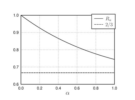
Figure 1: The left-hand and right-hand sides of (53) for real $\alpha\in(0;1]$.

VI Conclusion

We have obtained new uncertainty and certainty relations for the Pauli observables in terms of the Tsallis $\alpha$-entropies. These entropies form an especially important one-parametric extension of the Shannon entropy. The uncertainty and certainty relations are respectively expressed as lower and upper bounds on the sum of three $\alpha$-entropies. Lower bounds on the entropic sum are given for arbitrary $\alpha>0$. For real $\alpha\in(0;1]$ and integer $\alpha\geq 2$, the presented bounds are tight in the sense that they can certainly be saturated. The conditions for equality in the relations are obtained as well. For non-integer $\alpha>1$, we have presented approximate lower bounds on the entropic sum. Approximate bounds are based on the tight bounds for integer $\alpha$ and concavity properties with respect to the parameter $\alpha$. In the case of pure states, tight upper bounds on the sum have been obtained for all $\alpha\in(0;1]$ and integer $\alpha\geq 2$. These bounds have previously been explained with some intuitive reasons. Our method seems to be insufficient for obtaining upper bounds with non-integer $\alpha>1$. In principle, this issue could be studied by direct numerical calculations. Indeed, nonlinear optimization problems with no immediate solution are often arisen in maximizing information-theoretical quantities fperes96 . We also note that our results were all tested numerically. For any number of mutually unbiased bases in finite dimensions, lower bounds on the sum of Shannon entropies have been derived in molm09 . Bounds of such a kind could be obtained with use of Tsallis’ entropies. This issue will be considered in a following work.

- (1) Heisenberg, W.: Über den anschaulichen Inhalt der quanten theoretischen Kinematik und Mechanik, Zeitschrift für Physik 43, 172–198 (1927). Reprinted In: Wheeler, J.A., Zurek, W.H. (eds.): Quantum Theory and Measurement, 62–84. Princeton University Press, Princeton (1983)
- (2) Hall, M.J.W.: Universal geometric approach to uncertainty, entropy, and information. Phys. Rev. A 59, 2602–2615 (1999)
- (3) Busch, P., Heinonen, T., Lahti, P.J.: Heisenberg’s uncertainty principle. Phys. Rep. 452, 155–176 (2007)
- (4) Damgård, I., Fehr, S., Renner, R., Salvail, L., Schaffner, C.: A tight high-order entropic quantum uncertainty relation with applications. In: Advances in Cryptology – CRYPTO ’07, Lecture Notes in Computer Science, vol. 4622, 360–378. Springer, Berlin (2007)
- (5) Renes, J.M., Boileau, J.-C.: Conjectured strong complementary information tradeoff. Phys. Rev. Lett. 103, 020402 (2009)
- (6) Ver Steeg, G., Wehner, S.: Relaxed uncertainty relations and information processing. Quantum Information & Computation 9, 0801–0832 (2009)
- (7) Wehner, S., Winter, A.: Entropic uncertainty relations – a survey. New J. Phys. 12, 025009 (2010)
- (8) Białynicki-Birula, I., Rudnicki, Ł.: Entropic uncertainty relations in quantum physics. In Sen, K.D. (ed.): Statistical Complexity, 1–34. Springer, Berlin (2011)
- (9) Robertson, H.P.: The uncertainty principle. Phys. Rev. 34, 163–164 (1929)
- (10) Deutsch, D.: Uncertainty in quantum measurements. Phys. Rev. Lett. 50, 631–633 (1983)
- (11) Maassen, H., Uffink, J.B.M.: Generalized entropic uncertainty relations. Phys. Rev. Lett. 60, 1103–1106 (1988)
- (12) Kraus, K.: Complementary observables and uncertainty relations. Phys. Rev. D 35, 3070–3075 (1987)
- (13) Krishna, M., Parthasarathy, K.R.: An entropic uncertainty principle for quantum measurements. Sankhyā, Ser. A 64, 842 851 (2002)
- (14) Rastegin, A.E.: Rényi formulation of the entropic uncertainty principle for POVMs. J. Phys. A: Math. Theor. 43, 155302 (2010)
- (15) Ambainis, A.: Limits on entropic uncertainty relations. Quantum Information & Computation 10, 0848–0858 (2010)
- (16) Ng, H.Y.N., Berta, M., Wehner, S.: Min-entropy uncertainty relation for finite-size cryptography. Phys. Rev. A 86, 042315 (2012)
- (17) Ivanovic, I.D.: An inequality for the sum of entropies of unbiased quantum measurements. J. Phys. A: Math. Gen. 25, L363–L364 (1992)
- (18) Sánchez, J.: Entropic uncertainty and certainty relations for complementary observables. Phys. Lett. A 173, 233–239 (1993)
- (19) Sánchez-Ruiz, J.: Improved bounds in the entropic uncertainty and certainty relations for complementary observables. Phys. Lett. A 201, 125–131 (1995)
- (20) Wu, S., Yu, S., Mølmer, K.: Entropic uncertainty relation for mutually unbiased bases. Phys. Rev. A 79, 022104 (2009)
- (21) Wehner, S., Winter, A.: Higher entropic uncertainty relations for anti-commuting observables. J. Math. Phys. 49, 062105 (2008)
- (22) Rényi, A.: On measures of entropy and information. In: Neyman J. (ed), Proceedings of 4th Berkeley symposium on mathematical statistics and probability. Vol. I, 547 -561. University of California Press, Berkeley (1961)
- (23) Tsallis, C.: Possible generalization of Boltzmann–Gibbs statistics. J. Stat. Phys. 52, 479–487 (1988)
- (24) Bialynicki-Birula, I.: Formulation of the uncertainty relations in terms of the Rényi entropies. Phys. Rev. A 74, 052101 (2006)
- (25) Rastegin, A.E.: Entropic uncertainty relations for extremal unravelings of super-operators. J. Phys. A: Math. Theor. 44, 095303 (2011)
- (26) Rastegin, A.E.: Entropic formulation of the uncertainty principle for the number and annihilation operators. Phys. Scr. 84, 057001 (2011)
- (27) Berta, M., Christandl, M., Colbeck, R., Renes, J.M., Renner, R.: The uncertainty principle in the presence of quantum memory. Nature Physics 6, 659–662 (2010)
- (28) Coles, P.J., Yu, L., Zwolak, M.: Relative entropy derivation of the uncertainty principle with quantum side information. arXiv:1105.4865 [quant-ph] (2011)
- (29) Hu, M.-L., Fan, H.: Competition between quantum correlations in the quantum-memory-assisted entropic uncertainty relation. Phys. Rev. A 87, 022314 (2013)
- (30) Rastegin, A.E.: Entropic uncertainty relations and quasi-Hermitian operators. J. Phys. A: Math. Theor. 45, 444026 (2012)
- (31) Hu, X., Ye, Z.: Generalised quantum entropies. J. Math. Phys. 47, 023502 (2006)
- (32) Larsen, U.: Superspace geometry: the exact uncertainty relationship between complementarity aspects. J. Phys. A: Math. Gen. 23, 1041–1061 (1990)
- (33) Garcia Diaz, R., Romero, J.L., Björk, G., Bourennane, M.: Certainty relations between local and nonlocal observables. New J. Phys. 7, 256 (2005)
- (34) Rastegin, A.E.: Number-phase uncertainty relations in terms of generalized entropies. Quantum Information & Computation 12, 0743–0762 (2012)
- (35) Rastegin, A.E.: Notes on entropic uncertainty relations beyond the scope of Riesz’s theorem. Int. J. Theor. Phys. 51, 1300–1315 (2011)
- (36) Berta, M., Fawzi, O., Wehner, S.: Quantum to classical randomness extractors. arXiv:1111.2026 [quant-ph] (2011)
- (37) Havrda, J., Charvát, F.: Quantification methods of classification processes: concept of structural -entropy. Kybernetika 3, 30–35 (1967)
- (38) Bengtsson, I., Życzkowski, K.: Geometry of Quantum States: An Introduction to Quantum Entanglement. Cambridge University Press, Cambridge (2006)
- (39) Fuchs, C.A., Peres, A.: Quantum state disturbance versus information gain: uncertainty relations for quantum information. Phys. Rev. A 53, 2038–2045 (1996)