Scale coupling and interface pinning effects in the phase-field-crystal model

Abstract

Effects of scale coupling between mesoscopic slowly-varying envelopes of liquid-solid profile and the underlying microscopic crystalline structure are studied in the phase-field-crystal (PFC) model. Such scale coupling leads to nonadiabatic corrections to the PFC amplitude equations, the effect of which increases strongly with decreasing system temperature below the melting point. This nonadiabatic amplitude representation is further coarse-grained for the derivation of effective sharp-interface equations of motion in the limit of small but finite interface thickness. We identify a generalized form of the Gibbs-Thomson relation with the incorporation of coupling and pinning effects of the crystalline lattice structure. This generalized interface equation can be reduced to the form of a driven sine-Gordon equation with KPZ nonlinearity, and be combined with other two dynamic equations in the sharp interface limit obeying the conservation condition of atomic number density in a liquid-solid system. A sample application to the study of crystal layer growth is given, and the corresponding analytic solutions showing lattice pinning and depinning effects and two distinct modes of continuous vs. nucleated growth are presented. We also identify the universal scaling behaviors governing the properties of pinning strength, surface tension, interface kinetic coefficient, and activation energy of atomic layer growth, which accommodate all range of liquid-solid interface thickness and different material elastic modulus.

I Introduction

Continuum theories have been playing a continuously important role in modeling and understanding a wide range of complex nonequilibrium phenomena during materials growth and processing. For the typical example of liquid-solid front motion and interface growth, sharp-interface or Stefan-type models have been used in early studies to examine various solidification phenomena such as dendritic growth and directional solidification of either pure systems or eutectic alloys Langer (1980). Recent focus has been put on the continuum phase-field approach, which has become a widely-adopted method in materials modeling not only due to its computational advantage as compared to atomistic techniques and also to the complex moving-boundary problems encountered in sharp-interface models, but also due to its vast applicability for a wide variety of material phenomena including solidification, phase transformation, alloy decomposition, nucleation, defects evolution, nanostructure formation, etc. Elder et al. (1994); Karma and Rappel (1998); Elder et al. (2001); Müller and Grant (1999); Kassner et al. (2001); Granasy et al. (2004); Wang and Li (2010).

These continuum methods are well formulated for the description of long wavelength behavior of a system. To incorporate properties related to smaller-scale crystalline details which can have significant impact, additional assumptions or modifications are required. Examples include the consideration of lattice anisotropy for surface tension and kinetics Karma and Rappel (1998), and the incorporation of subsidiary fields describing system elasticity Müller and Grant (1999); Kassner et al. (2001), plasticity Wang and Li (2010), or local crystal orientation Granasy et al. (2004) in phase-field models. However, effects associated with the discreteness of a crystalline system, such as the atomistic feature of lattice growth, are usually absent due to the nature of continuum description. Efforts to partially remedy this in some previous studies include, e.g., the adding of a periodic potential mimicking effects of crystalline lattice along the growth direction in the continuum modeling of surface roughening transition Chui and Weeks (1978); Nozières and Gallet (1987); Hwa et al. (1991); *re:balibar92; *re:mikheev93; *re:rost94; *re:hwa94, although both the form of lattice potential (usually assumed as a sinusoidal function as part of the sine-Gordon Hamiltonian) and the associated parameters were introduced phenomenologically.

More systematic approaches based on some fundamental microscopic-level theories are needed for the construction of continuum field models that incorporate crystalline/atomistic features. One of the recent advances on this front is the development of phase-field-crystal (PFC) methods Elder et al. (2002); *re:elder04; Elder et al. (2007), in which the structure and dynamics of a solid system are described by a continuum local atomic density field that is spatially periodic and of atomistic resolution; thus the small length scale of crystalline lattice structure is intrinsically built into the continuum field description with diffusive dynamic time scales. Both free energy functionals and dynamics of the PFC models can be derived from atomic-scale theory through classical density functional theory of freezing (CDFT) and the corresponding dynamic theory (DDFT), for both single-component and alloy systems Elder et al. (2007); Huang et al. (2010); Greenwood et al. (2010); *re:greenwood11b; van Teeffelen et al. (2009); Jaatinen et al. (2009). Properties associated with crystalline nature of the system, such as elasticity, plasticity, multiple grain orientations, crystal symmetries and anisotropy, are then naturally included, with no additional phenomenological assumptions needed as compared to conventional continuum field theories. This advantage has been verified in a large variety of applications of PFC, ranging from structural, compositional, to nanoscale phenomena for both solid materials Elder et al. (2002); *re:elder04; Elder et al. (2007); Huang et al. (2010); Greenwood et al. (2010); *re:greenwood11b; Jaatinen et al. (2009); Huang and Elder (2008); *re:huang10; Wu and Voorhees (2009); Spatschek and Karma (2010); Muralidharan and Haataja (2010); Berry and Grant (2011); Elder et al. (2012) and soft matters van Teeffelen et al. (2009); Wittkowski et al. (2011).

An important feature of the PFC methodology is the multiple scale description it provides, as can be seen from its amplitude representation. The system dynamics is described by the behavior of “slow”-scale (mesoscopic) amplitudes/envelopes of the underlying crystalline lattice, as a result of the amplitude expansion of PFC density field in either pure liquid-solid systems Goldenfeld et al. (2005); *re:athreya06; Yeon et al. (2010) or binary alloys Elder et al. (2010); Huang et al. (2010); Spatschek and Karma (2010). Note that in these amplitude equation studies, although most lattice effects have been incorporated in the variation of complex amplitudes (mainly via their phase dynamics Huang and Elder (2008); *re:huang10), the spatial scales of the mesoscopic amplitudes and the microscopic lattice structure are assumed to be separated (i.e., the assumption of “adiabatic” expansion). However, this assumption only holds in the region of slowly varying density profile either close to the bulk state or for diffuse interfaces, and hence is valid only at high enough system temperature. In low or intermediate temperature regime showing sharp liquid-solid or grain-grain interfaces, amplitude variation around the interface would be of order close to the lattice periodicity; thus the two scales of amplitudes vs. lattice can no longer be separated, resulting in the “nonadiabatic” effect due to their coupling and interaction. Such scale coupling leads to an important effect of lattice pinning that plays a pivotal role in material growth and evolution, as first discussed by Pomeau Pomeau (1986) and later demonstrated in the phenomena of fluid convection and pattern formation Bensimon et al. (1988); Boyer and Viñals (2002a); *re:boyer02b. To our knowledge, these scale coupling effects have not been addressed explicitly in all previous phase-field and PFC studies of solidification and crystal growth.

In this paper we aim to identify these coupling effects between mesoscale structural amplitudes and the underlying microscopic spatial scale of crystalline structure, via deriving the nonadiabatic amplitude representation of the PFC model. What we study here is the simplest PFC system: two-dimensional (2D), single-component, and of hexagonal crystalline symmetry, as our main focus is on examining the fundamental aspects of scale coupling and bridging that are missing in previous research, and also on further completing the multi-scale features of the PFC methodology. The explicit expression of the resulting pinning force during liquid-solid interface motion, and also its scaling behavior with respect to the interface thickness, are determined in this work, through the application of sharp/thin interface approach (given finite interface thickness) to the amplitude equations. This leads to a new set of interface equations of motion, in particular a generalized Gibbs-Thomson relation that incorporates the pinning term and also its reduced form of a driven sine-Gordon equation. The pinning of the interface to the underlying crystalline lattice structure, and the associated nonactivated vs. nucleated growth modes, can be determined from analytic solutions of the interface equations for the case of planar layer growth.

II Nonadiabatic coupling in amplitude equations

In the PFC model for single-component systems, the dynamics of a rescaled atomic number density field $n({\bm{r}},t)$ is described in a dimensionless form Elder et al. (2002); *re:elder04; Elder et al. (2007); Huang et al. (2010)

$$\partial n/\partial t=\nabla^{2}\left[-\epsilon n+(\nabla^{2}+q_{0}^{2})^{2}n-gn^{2}+n^{3}\right]+{\bm{\nabla}}\cdot{\bm{\eta}},$$ (1)

where $\epsilon$ measures the temperature distance from the melting point, $g=(3/B^{x})^{1/2}/2$ with $B^{x}$ proportional to the bulk modulus, and we have $q_{0}=1$ after rescaling over a length scale $R$ of lattice spacing. The noise field ${\bm{\eta}}$ has zero mean and obeys the correlations

$$\langle\eta^{\alpha}({\bm{r}},t)\eta^{\beta}({\bm{r}^{\prime}},t^{\prime})\rangle=2\Gamma_{0}k_{B}T\delta({\bm{r}}-{\bm{r}^{\prime}})\delta(t-t^{\prime})\delta^{\alpha\beta}$$ (2)

with $\alpha,\beta=x,y,z$, where $\Gamma_{0}$ is a rescaled constant depending on $B^{x}$ and $R$ Huang et al. (2010), and $T$ is the system temperature.

To derive the corresponding 2D amplitude equations in the limit of small $\epsilon$, we need to first distinguish the “slow” spatial and temporal scales for the amplitudes/envelopes of the structural profile, i.e.,

$$X=\epsilon^{1/2}x,\qquad Y=\epsilon^{1/2}y,\qquad T=\epsilon t,$$ (3)

from the “fast” scales $(x,y,t)$ of the underlying hexagonal crystalline structure. We then expand the PFC model equation (1) based on this scale separation and also on a hybrid approach combining the standard multiple-scale expansionManneville (1990); Cross and Hohenberg (1993) and the idea of “Quick-and-Dirty” renormalization group method Goldenfeld et al. (2005); *re:athreya06 (see Ref. Huang et al. (2010) for details). To incorporate the coupling between these “slow” and “fast” scales, which leads to nonadiabatic corrections to the amplitude equations, we use an approach based on that given in Refs. Bensimon et al. (1988); Boyer and Viñals (2002a); *re:boyer02b which address front motion and locking in periodic pattern formation during fluid convection.

Following the steps of standard multiple-scale analysis Manneville (1990); Cross and Hohenberg (1993), the atomic density field $n$ can be expanded as

$$n=n_{0}(X,Y,T)+\sum\limits_{j=1}^{3}A_{j}(X,Y,T)e^{i{\bm{q}}_{j}^{0}\cdot{\bm{r}}}+\text{c.c.},$$ (4)

where ${\bm{q}}_{j}^{0}$ are the three basic wave vectors for 2D hexagonal structure (i.e., the 3 “fast”-scale base modes)

$${\bm{q}_{1}^{0}}=-q_{0}\left(\frac{\sqrt{3}}{2}\hat{x}+\frac{\hat{y}}{2}\right),{\bm{q}_{2}^{0}}=q_{0}\hat{y},{\bm{q}_{3}^{0}}=q_{0}\left(\frac{\sqrt{3}}{2}\hat{x}-\frac{\hat{y}}{2}\right),$$ (5)

and the slow scaled fields, including $A_{j}$ (complex amplitudes of mode ${\bm{q}}_{j}^{0}$) and $n_{0}$ (real amplitude of the zero wavenumber neutral mode as a result of PFC conserved dynamics), are represented as power series of $\epsilon$: $A_{j}=\epsilon^{1/2}A_{j}^{(1/2)}+\epsilon A_{j}^{(1)}+\epsilon^{3/2}A_{j}^{(3/2)}+\cdots=\sum_{m=1}^{\infty}\epsilon^{m/2}A_{j}^{(m/2)}$, $n_{0}=\epsilon^{1/2}n_{0}^{(1/2)}+\epsilon n_{0}^{(1)}+\epsilon^{3/2}n_{0}^{(3/2)}+\cdots=\sum_{m=1}^{\infty}\epsilon^{m/2}n_{0}^{(m/2)}$. Note that in Eq. (4) higher harmonic terms have been neglected.

From Eqs. (3) and (4) as well as the substitutions $\partial_{x(y)}\rightarrow\partial_{x(y)}+\epsilon^{1/2}\partial_{X(Y)}$ and $\partial_{t}\rightarrow\epsilon\partial_{T}$, we obtain the following expansion for the PFC equation (1) in the absence of noise:

$$\left[\mathcal{L}n+\nabla^{2}\left(gn^{2}-n^{3}\right)\right]_{s} =\epsilon\partial_{T}n_{0}-\epsilon\nabla_{s}^{2}\frac{\delta\mathcal{F}_{s}}{\delta n_{0}}+\sum_{j=1}^{3}\left[\left(\epsilon\partial_{T}A_{j}-\mathcal{L}_{j}^{s}\frac{\delta\mathcal{F}_{s}}{\delta A_{j}^{*}}\right)e^{i{\bm{q}}_{j}^{0}\cdot{\bm{r}}}+\text{c.c.}\right]$$ (6)

$$+\left[f_{p_{11}}e^{2i{\bm{q}}_{1}^{0}\cdot{\bm{r}}}+f_{p_{2}}e^{2i{\bm{q}}_{2}^{0}\cdot{\bm{r}}}+f_{p_{33}}e^{2i{\bm{q}}_{3}^{0}\cdot{\bm{r}}}+f_{p_{1}}e^{i({\bm{q}}_{1}^{0}-{\bm{q}}_{2}^{0})\cdot{\bm{r}}}+f_{p_{0}}e^{i({\bm{q}}_{1}^{0}-{\bm{q}}_{3}^{0})\cdot{\bm{r}}}+f_{p_{3}}e^{i({\bm{q}}_{3}^{0}-{\bm{q}}_{2}^{0})\cdot{\bm{r}}}+\text{c.c.}\right]$$

$$+\sum_{j\neq k=1}^{3}f_{p_{jk}}e^{i(2{\bm{q}}_{j}^{0}-{\bm{q}}_{k}^{0})\cdot{\bm{r}}}+9q_{0}^{2}\sum_{j=1}^{3}A_{j}^{3}e^{3i{\bm{q}}_{j}^{0}\cdot{\bm{r}}}+\text{c.c.},$$

where $\mathcal{L}=\partial_{t}+\epsilon\nabla^{2}-\nabla^{2}(\nabla^{2}+q_{0}^{2})^{2}$ is the linear operator in PFC, $[\cdots]_{s}$ refers to the slow-scale expansion to all orders of $\epsilon$, and $\bm{\nabla}_{s}=(\partial_{X},\partial_{Y})$, $\nabla_{s}^{2}=\partial_{X}^{2}+\partial_{Y}^{2}$, and $\mathcal{L}_{j}^{s}=\epsilon\nabla_{s}^{2}+\epsilon^{1/2}\left(2i{\bm{q}}_{j}^{0}\cdot{\bm{\nabla}}_{s}\right)-q_{0}^{2}$ are slow operators. In Eq. (6), $\mathcal{F}_{s}$ is the slow-scale correspondence of the effective free energy $\mathcal{F}$ given below [with $(\nabla^{2}+2i{\bm{q}}_{j}^{0}\cdot{\bm{\nabla}})$ replaced by $(\mathcal{L}_{j}^{s}+q_{0}^{2})$ and $(\nabla^{2}+q_{0}^{2})$ replaced by $(\epsilon\nabla_{s}^{2}+q_{0}^{2})$]:

$$\mathcal{F}= \int d\bm{r}\left\{(-\epsilon+3n_{0}^{2}-2gn_{0})\sum_{j=1}^{3}|A_{j}|^{2}\right.$$ (7)

$$+\sum_{j=1}^{3}\left|\left(\nabla^{2}+2i{\bm{q}}_{j}^{0}\cdot{\bm{\nabla}}\right)A_{j}\right|^{2}+\frac{3}{2}\sum_{j=1}^{3}|A_{j}|^{4}$$

$$+(6n_{0}-2g)\left(\prod_{j=1}^{3}A_{j}+\text{c.c.}\right)+6\sum_{j<k}|A_{j}|^{2}|A_{k}|^{2}$$

$$\left.-\frac{1}{2}\epsilon n_{0}^{2}+\frac{1}{2}\left[\left(\nabla^{2}+q_{0}^{2}\right)n_{0}\right]^{2}-\frac{1}{3}gn_{0}^{3}+\frac{1}{4}n_{0}^{4}\right\},$$

which is the same as the previous amplitude expansion result Yeon et al. (2010); Huang and Elder (2008); *re:huang10; Huang et al. (2010); also for other variables $f_{p_{jk}}$ ($j,k=1,2,3$) and $f_{p_{i}}$ ($i=0,...,3$) related to higher harmonics,

$$f_{p_{1}} =3q_{0}^{2}\left[(6n_{0}-2g)A_{1}A_{2}^{*}+3\left(A_{1}^{2}A_{3}+{A_{2}^{*}}^{2}A_{3}^{*}\right)\right],$$

$$f_{p_{2}} =4q_{0}^{2}\left[(3n_{0}-g)A_{2}^{2}+6A_{1}^{*}A_{2}A_{3}^{*}\right],$$

$$f_{p_{3}} =3q_{0}^{2}\left[(6n_{0}-2g)A_{2}^{*}A_{3}+3\left(A_{1}A_{3}^{2}+A_{1}^{*}{A_{2}^{*}}^{2}\right)\right],$$

$$f_{p_{0}} =3q_{0}^{2}\left[(6n_{0}-2g)A_{1}A_{3}^{*}+3\left(A_{1}^{2}A_{2}+A_{2}^{*}{A_{3}^{*}}^{2}\right)\right],$$

$$f_{p_{11}} =4q_{0}^{2}\left[(3n_{0}-g)A_{1}^{2}+6A_{1}A_{2}^{*}A_{3}^{*}\right],$$

$$f_{p_{33}} =4q_{0}^{2}\left[(3n_{0}-g)A_{3}^{2}+6A_{1}^{*}A_{2}^{*}A_{3}\right],$$

$$f_{p_{jk}} =21q_{0}^{2}A_{j}^{2}A_{k}^{*}~{}~{}(j\neq k).$$ (8)

As in the hybrid method developed in Ref. Huang et al. (2010), the amplitude equations governing $A_{j}$ and $n_{0}$ can be derived from the integration of Eq. (6) over eigenmodes $\{e^{-i{\bm{q}}_{j}^{0}\cdot{\bm{r}}},1\}$, i.e.,

$$\int_{x}^{x+\lambda_{x}}\frac{dx^{\prime}}{\lambda_{x}}\int_{y}^{y+\lambda_{y}}\frac{dy^{\prime}}{\lambda_{y}}\left[\mathcal{L}n+\nabla^{2}(gn^{2}-n^{3})\right]_{s}e^{-i{\bm{q}}_{j}^{0}\cdot{\bm{r}^{\prime}}}=0,$$

$$\int_{x}^{x+\lambda_{x}}\frac{dx^{\prime}}{\lambda_{x}}\int_{y}^{y+\lambda_{y}}\frac{dy^{\prime}}{\lambda_{y}}\left[\mathcal{L}n+\nabla^{2}(gn^{2}-n^{3})\right]_{s}=0,$$ (9)

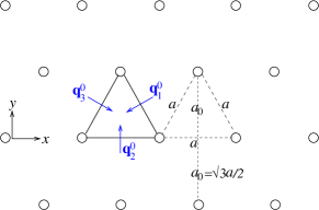
where $\lambda_{x}=a=a_{0}/(\sqrt{3}/2)$ and $\lambda_{y}=\sqrt{3}a=2a_{0}$ (with $a$ the atomic lattice spacing for the hexagonal/triangular structure and $a_{0}=2\pi/q_{0}$, as illustrated in Fig. 1), which are the atomic spatial periods along the $x$ and $y$ directions respectively. Note that Eq. (9) can be also viewed as the combination of the solvability conditions obtained at all different orders of $\epsilon$ in multiple-scale expansion Huang et al. (2010).

Figure 1: (Color online) Schematic of a hexagonal/triangular lattice, with atomic lattice spacing $a=a_{0}/(\sqrt{3}/2)$, $a_{0}=2\pi/q_{0}$, and 3 basic wave vectors ${\bm{q}}_{j}^{0}$ ($j=1,2,3$) expressed in Eq. (5).

In the limit of $\epsilon\rightarrow 0$, i.e., close to the melting temperature, the spatial variation of amplitudes $A_{j}(X,Y,T)$ and $n_{0}(X,Y,T)$ is of much larger scale compared to the atomic lattice variation scales $\lambda_{x}$ and $\lambda_{y}$. Thus “slow” and “fast” length scales in the integral of Eq. (9) can be separated as in standard multiple-scale analysis (i.e., $(X,Y)$ and $(x,y)$ be treated as independent variables), leading to the Ginzburg-Landau-type amplitude equations obtained in previous studies Yeon et al. (2010); Huang and Elder (2008):

$$\partial A_{j}/\partial t=\mathcal{L}_{j}\frac{\delta\mathcal{F}}{\delta A_{j}^{*}}\simeq-q_{0}^{2}\frac{\delta\mathcal{F}}{\delta A_{j}^{*}},\quad\partial n_{0}/\partial t=\nabla^{2}\frac{\delta\mathcal{F}}{\delta n_{0}}.$$ (10)

Note that to derive Eq. (10) the long-wavelength approximation $\mathcal{L}_{j}=\nabla^{2}+2i{\bm{q}}_{j}^{0}\cdot{\bm{\nabla}}-q_{0}^{2}\simeq-q_{0}^{2}$ has been used as before.

However, such assumption of scale separation would not hold when $\epsilon$ is of larger value (still small but finite, corresponding to low/moderate material temperature far enough from the melting point). Although the amplitudes/envelopes still vary slowly in the bulk, the interface, either between liquid and solid states or between different grains, could be thin or sharp, with its width comparable to “fast” lattice scales (e.g., of few lattice spacings). Thus functions of $A_{j}$ and $n_{0}$ in Eq. (6) can no longer be decoupled from the atomic-scale oscillatory terms $e^{i(l{\bm{q}}_{j}^{0}-m{\bm{q}}_{k}^{0})\cdot{\bm{r}}}$ (with $l$ and $m$ integers and $j,k=1,2,3$) in the integration of $\int_{x}^{x+\lambda_{x}}dx^{\prime}\int_{y}^{y+\lambda_{y}}dy^{\prime}$ in Eq. (9). Using an approximation similar to that in Ref. Boyer and Viñals (2002a); *re:boyer02b, we only keep the lowest-order coupling terms, i.e., terms coupled to lowest modes (with largest atomic lengths) along both $x$ and $y$ directions, including $e^{i{\bm{q}}_{j}^{0}\cdot{\bm{r}}}$, corresponding to atomic layer spacing $\sqrt{3}a/2=a_{0}$, and $e^{i({\bm{q}}_{j}^{0}-{\bm{q}}_{k}^{0})_{j\neq k}\cdot{\bm{r}}}$, with atomic layer spacing $a/2=a_{0}/\sqrt{3}$. Couplings to higher modes, such as $e^{2i{\bm{q}}_{j}^{0}\cdot{\bm{r}}}$ (with length scale $a_{0}/2$), $e^{i(2{\bm{q}}_{j}^{0}-{\bm{q}}_{k}^{0})_{j\neq k}\cdot{\bm{r}}}$ (with length scale $a_{0}/\sqrt{7}$), etc., are neglected. The following scale-coupled amplitude equations can then be derived from Eqs. (9) and (6):

$$\partial A_{1}/\partial t= -q_{0}^{2}\frac{\delta\mathcal{F}}{\delta A_{1}^{*}}$$ (11)

$$-\frac{1}{\lambda_{x}\lambda_{y}}\int_{x}^{x+\lambda_{x}}dx^{\prime}\int_{y}^{y+\lambda_{y}}dy^{\prime}\left[f_{p_{1}}e^{-iq_{0}y^{\prime}}+f_{p_{11}}e^{-iq_{0}\left(\frac{\sqrt{3}}{2}x^{\prime}+\frac{1}{2}y^{\prime}\right)}+f_{p_{0}}e^{iq_{0}\left(-\frac{\sqrt{3}}{2}x^{\prime}+\frac{1}{2}y^{\prime}\right)}\right.$$

$$\left.+f_{p_{13}}e^{-iq_{0}\sqrt{3}x^{\prime}}+f_{p_{12}}e^{-iq_{0}\left(\frac{\sqrt{3}}{2}x^{\prime}+\frac{3}{2}y^{\prime}\right)}+f^{*}_{p_{2}}e^{iq_{0}\left(\frac{\sqrt{3}}{2}x^{\prime}-\frac{3}{2}y^{\prime}\right)}+f^{*}_{p_{33}}e^{iq_{0}\left(-\frac{\sqrt{3}}{2}x^{\prime}+\frac{3}{2}y^{\prime}\right)}\right]+\eta_{1},$$

$$\partial A_{2}/\partial t= -q_{0}^{2}\frac{\delta\mathcal{F}}{\delta A_{2}^{*}}$$ (12)

$$-\frac{1}{\lambda_{x}\lambda_{y}}\int_{x}^{x+\lambda_{x}}dx^{\prime}\int_{y}^{y+\lambda_{y}}dy^{\prime}\left[f_{p_{2}}e^{iq_{0}y^{\prime}}+f^{*}_{p_{1}}e^{iq_{0}\left(\frac{\sqrt{3}}{2}x^{\prime}+\frac{1}{2}y^{\prime}\right)}+f^{*}_{p_{3}}e^{iq_{0}\left(-\frac{\sqrt{3}}{2}x^{\prime}+\frac{1}{2}y^{\prime}\right)}\right.$$

$$\left.+f^{*}_{p_{11}}e^{iq_{0}\sqrt{3}x^{\prime}}+f^{*}_{p_{33}}e^{-iq_{0}\sqrt{3}x^{\prime}}+f_{p_{21}}e^{iq_{0}\left(\frac{\sqrt{3}}{2}x^{\prime}+\frac{3}{2}y^{\prime}\right)}+f_{p_{23}}e^{iq_{0}\left(-\frac{\sqrt{3}}{2}x^{\prime}+\frac{3}{2}y^{\prime}\right)}\right]+\eta_{2},$$

$$\partial A_{3}/\partial t= -q_{0}^{2}\frac{\delta\mathcal{F}}{\delta A_{3}^{*}}$$ (13)

$$-\frac{1}{\lambda_{x}\lambda_{y}}\int_{x}^{x+\lambda_{x}}dx^{\prime}\int_{y}^{y+\lambda_{y}}dy^{\prime}\left[f_{p_{3}}e^{-iq_{0}y^{\prime}}+f^{*}_{p_{0}}e^{iq_{0}\left(\frac{\sqrt{3}}{2}x^{\prime}+\frac{1}{2}y^{\prime}\right)}+f_{p_{33}}e^{iq_{0}\left(\frac{\sqrt{3}}{2}x^{\prime}-\frac{1}{2}y^{\prime}\right)}\right.$$

$$\left.+f_{p_{31}}e^{iq_{0}\sqrt{3}x^{\prime}}+f^{*}_{p_{11}}e^{iq_{0}\left(\frac{\sqrt{3}}{2}x^{\prime}+\frac{3}{2}y^{\prime}\right)}+f^{*}_{p_{2}}e^{-iq_{0}\left(\frac{\sqrt{3}}{2}x^{\prime}+\frac{3}{2}y^{\prime}\right)}+f_{p_{32}}e^{iq_{0}\left(\frac{\sqrt{3}}{2}x^{\prime}-\frac{3}{2}y^{\prime}\right)}\right]+\eta_{3},$$

$$\partial n_{0}/\partial t= \nabla^{2}\frac{\delta\mathcal{F}}{\delta n_{0}}$$ (14)

$$-\frac{1}{\lambda_{x}\lambda_{y}}\int_{x}^{x+\lambda_{x}}dx^{\prime}\int_{y}^{y+\lambda_{y}}dy^{\prime}\left[f^{*}_{p_{0}}e^{iq_{0}\sqrt{3}x^{\prime}}+f^{*}_{p_{1}}e^{iq_{0}\left(\frac{\sqrt{3}}{2}x^{\prime}+\frac{3}{2}y^{\prime}\right)}+f_{p_{3}}e^{iq_{0}\left(\frac{\sqrt{3}}{2}x^{\prime}-\frac{3}{2}y^{\prime}\right)}+\text{c.c.}\right]+\bm{\nabla}\cdot\bm{\eta}_{0},$$

where a projection procedure has been applied to address the noise term of the PFC Eqs. (1) and (2) Huang et al. (2010), leading to zero mean of noise amplitudes $\eta_{j}$ and $\bm{\eta}_{0}$, as well as the correlations $\langle\eta_{i}\eta_{j}\rangle=\langle{\bm{\eta}}_{0}\eta_{j}\rangle=\langle{\bm{\eta}}_{0}\eta_{j}^{*}\rangle=0$ and

$$\langle\eta_{i}\eta_{j}^{*}\rangle=2\vartheta_{i}q_{0}^{2}\Gamma_{0}k_{B}T\delta({\bm{r}}-{\bm{r}^{\prime}})\delta(t-t^{\prime})\delta_{ij},$$

$$\langle\eta_{0}^{\alpha}\eta_{0}^{\beta}\rangle=2\vartheta_{0}\Gamma_{0}k_{B}T\delta({\bm{r}}-{\bm{r}^{\prime}})\delta(t-t^{\prime})\delta^{\alpha\beta},$$ (15)

with $i,j=1,2,3$, $\alpha,\beta=x,y$, and $\vartheta_{i}=\vartheta_{0}=1/7$ if assuming equal contribution from all eigenmodes $\{e^{i{\bm{q}}_{j}^{0}\cdot{\bm{r}}},1\}$. In the above generalized amplitude equations (11)–(14), the integration terms explicitly yield the coupling between “slow” (for structural amplitudes or envelopes) and “fast” (for atomic lattice variations) spatial scales, that is, the nonadiabatic corrections. The first 3 coupling terms in each of Eqs. (11)–(13) for the dynamics of complex amplitudes $A_{j}$ are associated with lattice modes $e^{i{\bm{q}}_{j}^{0}\cdot{\bm{r}}}$ of length scale $a_{0}$ ($=\sqrt{3}a/2$), while the other 4 terms correspond to the coupling to $e^{i({\bm{q}}_{j}^{0}-{\bm{q}}_{k}^{0})_{j\neq k}\cdot{\bm{r}}}$ modes with length scale $a_{0}/\sqrt{3}$ ($=a/2$). The nonadiabatic effect for $n_{0}$ dynamics is weaker, with only couplings to the $a_{0}/\sqrt{3}$ length scale given in Eq. (14). Note that in the bulk state of single crystal or homogeneous liquid, the amplitude functions $f_{p_{i}}$, $f_{p_{jk}}$ $\sim$ constants, and hence all the integrals in Eqs. (11)–(13) are equal to zero; we can then recover the original amplitude equations (10) without any nonadiabatic coupling, as expected.

III Interface equations of motion with lattice pinning

To illustrate the important effects of scale coupling identified in above nonadiabatic amplitude equations, here we consider a system of coexisting liquid and solid phases, with the average interface normal direction pointed along $\hat{y}$. The extension of our derivation and results to other interface orientations is straightforward.

In this case, the “slow” and “fast” scales parallel to the interface can be well separated, and to lowest-order approximation the amplitude equations (11)–(13) are rewritten as

$$\partial A_{j}/\partial t = -q_{0}^{2}\frac{\delta\mathcal{F}}{\delta A_{j}^{*}}-\frac{1}{\lambda_{y}}\int_{y}^{y+\lambda_{y}}dy^{\prime}f_{p_{j}}e^{\mp iq_{0}y^{\prime}}+\eta_{j}$$ (16)

$$= -q_{0}^{2}\left[\left(\nabla^{2}+2i\bm{q}_{j}^{0}\cdot\bm{\nabla}\right)^{2}A_{j}+\frac{\partial f}{\partial A_{j}^{*}}\right]$$

$$-\frac{1}{\lambda_{y}}\int_{y}^{y+\lambda_{y}}dy^{\prime}f_{p_{j}}e^{\mp iq_{0}y^{\prime}}+\eta_{j},$$

$$\partial n_{0}/\partial t = \nabla^{2}\frac{\delta\mathcal{F}}{\delta n_{0}}+\bm{\nabla}\cdot\bm{\eta}_{0}=\nabla^{2}\mu+\bm{\nabla}\cdot\bm{\eta}_{0}$$ (17)

$$= \nabla^{2}\left[\left(\nabla^{4}+2q_{0}^{2}\nabla^{2}\right)n_{0}+\frac{\partial f}{\partial n_{0}}\right]+\bm{\nabla}\cdot\bm{\eta}_{0},$$

($e^{-iq_{0}y^{\prime}}$: for $A_{1}$ and $A_{3}$; $e^{+iq_{0}y^{\prime}}$: for $A_{2}$), where $\mu=\delta\mathcal{F}/\delta n_{0}$ is a chemical potential of the system, and $f$ is the bulk free energy density given from Eq. (7):

$$f= (-\epsilon+3n_{0}^{2}-2gn_{0})\sum_{j=1}^{3}|A_{j}|^{2}+\frac{3}{2}\sum_{j=1}^{3}|A_{j}|^{4}$$ (18)

$$+(6n_{0}-2g)\left(\prod_{j=1}^{3}A_{j}+\text{c.c.}\right)+6\sum_{j<k}|A_{j}|^{2}|A_{k}|^{2}$$

$$+\frac{1}{2}\left(-\epsilon+q_{0}^{4}\right)n_{0}^{2}-\frac{1}{3}gn_{0}^{3}+\frac{1}{4}n_{0}^{4}.$$

To derive the corresponding equations of motion for the interface with finite thickness $\xi$ (i.e., in the sharp/thin interface limit Karma and Rappel (1998); Elder et al. (2001)), we follow the general approach developed by Elder et al. Elder et al. (2001) with the use of projection operator method. In this approach, a small parameter $\varepsilon$ is introduced, which represents the role of the interface Péclet number, and the system is partitioned into two regions: an inner region around the interface, defined by $-\zeta<u<+\zeta$, and an outer region far from the interface (i.e., $|u|>\zeta$), where length $\zeta$ scales as $1\ll\zeta/\xi\ll\varepsilon^{-1}$, and $u$ is the component of a local curvilinear coordinate in the interface normal direction. In this curvilinear coordinate $(u,s)$, the two orthogonal unit vectors are defined as $\hat{n}=\hat{x}\sin\theta+\hat{y}\cos\theta$ (local normal of the interface) and $\hat{t}=\partial\hat{n}/\partial\theta$ (tangent to the interface), where $\theta$ is the angle between $\hat{n}$ and the $y$ axis; also

$$\bm{\nabla}=\hat{n}\partial_{u}+\hat{t}\frac{\partial_{s}}{1+u\kappa},$$

$$\nabla^{2}=\partial_{u}^{2}+\frac{\kappa}{1+u\kappa}\partial_{u}+\frac{\partial_{s}^{2}}{(1+u\kappa)^{2}}-\frac{u\partial_{s}\kappa}{(1+u\kappa)^{3}}\partial_{s},$$ (19)

with the local curvature $\kappa=\bm{\nabla}\cdot\hat{n}=\partial\theta/\partial s$.

III.1 Outer equations

In the outer region which is far enough from the interface and close to the bulk states, the scale coupling term in Eq. (16) can be neglected, and the slowly varying amplitude fields $A_{j}$ and $n_{0}$ depend on rescaled spatial variables $(\varepsilon u/\xi,\varepsilon s/\xi)$ and rescaled time $\varepsilon^{2}t$. Expanding the outer solution of amplitudes in powers of $\varepsilon$, i.e.,

$$A_{j}^{\text{out}}={A_{j}^{0}}^{\text{out}}+\varepsilon{\tilde{A}_{j}}^{\text{out}}+\cdots,n_{0}^{\text{out}}={n_{0}^{0}}^{\text{out}}+\varepsilon{\tilde{n}_{0}}^{\text{out}}+\cdots,$$

$$\mu^{\text{out}}=\mu_{0}^{\text{out}}+\varepsilon\tilde{\mu}_{1}^{\text{out}}+\cdots,$$ (20)

substituting them into Eqs. (16) and (17), and using the rescaling given above, we find that at $\mathcal{O}(1)$,

$$\left.\frac{\partial f}{\partial A_{j}^{*}}\right|_{0}^{\text{out}}=0,\quad\partial{n_{0}^{0}}^{\text{out}}/\partial t=\nabla^{2}\left.\frac{\partial f}{\partial n_{0}}\right|_{0}^{\text{out}}=\nabla^{2}\mu_{0}^{\text{out}},$$ (21)

and at $\mathcal{O}(\varepsilon)$,

$$\left.\frac{\partial f}{\partial A_{j}^{*}}\right|_{1}^{\text{out}}=0,\quad\partial{\tilde{n}_{0}}^{\text{out}}/\partial t=\nabla^{2}\left.\frac{\partial f}{\partial n_{0}}\right|_{1}^{\text{out}}=\nabla^{2}\tilde{\mu}_{1}^{\text{out}},$$ (22)

where “$|_{0}^{\text{out}}$” refers to replacing $(A_{j},n_{0})$ by $({A_{j}^{0}}^{\text{out}},{n_{0}^{0}}^{\text{out}})$ in the derivative $\partial f/\partial A_{j}^{*}$ or $\partial f/\partial n_{0}$, and “$|_{1}^{\text{out}}$” refers to the corresponding results up to 1st order of ${\tilde{A}_{j}}^{\text{out}}$ and ${\tilde{n}_{0}}^{\text{out}}$. Note that if assuming the system to be not far from a liquid-solid equilibrium state, Eq. (21) of $\mathcal{O}(1)$ yields the bulk equilibrium solutions of the uniform liquid ($u=+\infty$) or solid ($u=-\infty$) state

$${A_{j}^{0}}^{\text{out}}(u)\equiv A_{j}^{0}(\pm\infty),\quad{n_{0}^{0}}^{\text{out}}(u)\equiv n_{0}^{0}(\pm\infty),$$ (23)

with the corresponding equilibrium chemical potential $\mu_{\text{eq}}=\mu_{0}^{\text{out}}=(\partial f/\partial n_{0})|_{0}^{\text{out}}$.

III.2 Inner expansion and lattice coupling effect

For the inner region ($-\zeta<u<+\zeta$), the amplitudes and chemical potential can be also expanded as

$$A_{j}^{\text{in}}=A_{j}^{0}+\varepsilon\tilde{A}_{j}+\cdots,\quad n_{0}^{\text{in}}=n_{0}^{0}+\varepsilon\tilde{n}_{0}+\cdots,$$

$$\mu^{\text{in}}=\mu_{0}+\varepsilon\tilde{\mu}_{1}+\cdots.$$ (24)

Due to the presence of interface at $u=0$, the amplitudes are expected to vary rapidly along the normal direction $\hat{n}$ but slowly along the arclength $s$ of the interface, leading to the rescaling $(U,S)=(u/\xi,\varepsilon s/\xi)$. Considering small interface fluctuations and noise amplitude, we assume that $\kappa=\varepsilon\tilde{\kappa}/\xi$, $\theta=\varepsilon\tilde{\theta}$, $\eta_{j}=\varepsilon\tilde{\eta}_{j}$, and $\bm{\eta}_{0}=\varepsilon\tilde{\bm{\eta}}_{0}$. Thus from Eq. (19) we have $\bm{\nabla}\cdot\bm{\eta}_{0}=\varepsilon\partial_{U}\tilde{\eta}_{0}^{u}/\xi+\mathcal{O}(\varepsilon^{2})$, $\nabla^{2}=(\partial_{U}^{2}+\varepsilon\tilde{\kappa}\partial_{U})/\xi^{2}+\mathcal{O}(\varepsilon^{2})$, and $(\nabla^{2}+2i\bm{q}_{j}^{0}\cdot\bm{\nabla})^{2}=(\nabla^{2}+2i\bm{q}_{j}^{0}\cdot\bm{\nabla})_{0}^{2}+\varepsilon(\nabla^{2}+2i\bm{q}_{j}^{0}\cdot\bm{\nabla})_{1}^{2}+\mathcal{O}(\varepsilon^{2})$, where for $j=1,3$,

$$\left(\nabla^{2}+2i\bm{q}_{j}^{0}\cdot\bm{\nabla}\right)_{0}^{2}= \left(\partial_{U}^{2}-iq_{0}\xi\partial_{U}\right)^{2}/\xi^{4},$$

$$\left(\nabla^{2}+2i\bm{q}_{j}^{0}\cdot\bm{\nabla}\right)_{1}^{2}= \left[\mp i2\sqrt{3}q_{0}\xi\sin\tilde{\theta}~{}\partial_{U}(\partial_{U}^{2}-iq_{0}\xi\partial_{U})\right.$$ (25)

$$+\tilde{\kappa}\partial_{U}(2\partial_{U}^{2}-3q_{0}^{2}\xi^{2})\mp 2\sqrt{3}q_{0}^{2}\xi^{2}\partial_{U}\partial_{S}$$

$$\left.-2iq_{0}\xi(\tilde{\kappa}\pm\sqrt{3}\partial_{S})\partial_{U}^{2}\right]/\xi^{4},$$

and for $j=2$,

$$\left(\nabla^{2}+2i\bm{q}_{2}^{0}\cdot\bm{\nabla}\right)_{0}^{2}= \left(\partial_{U}^{2}+2iq_{0}\xi\partial_{U}\right)^{2}/\xi^{4},$$

$$\left(\nabla^{2}+2i\bm{q}_{2}^{0}\cdot\bm{\nabla}\right)_{1}^{2}= 2\tilde{\kappa}\partial_{U}^{2}(\partial_{U}+2iq_{0}\xi)/\xi^{4}.$$ (26)

To address the time relaxation of system in the inner region, as usual we use a coordinate frame co-moving with the interface at a normal velocity $v_{n}(s)=\varepsilon\xi\tilde{v}(S)+\mathcal{O}(\varepsilon^{2})$, and hence $\partial_{t}\rightarrow\partial_{t}-\bm{v}\cdot\bm{\nabla}=-\varepsilon\tilde{v}\partial_{U}+\mathcal{O}(\varepsilon^{2})$. The inner expansion of the nonadiabatic amplitude equations (16) and (17) can then be given by: For $\mathcal{O}(1)$,

$$\left(\nabla^{2}+2i\bm{q}_{j}^{0}\cdot\bm{\nabla}\right)_{0}^{2}A_{j}^{0}+\left.\frac{\partial f}{\partial A_{j}^{*}}\right|_{0}=0,$$

$$\partial_{U}^{2}\left[\frac{1}{\xi^{4}}\partial_{U}^{2}\left(\partial_{U}^{2}+2q_{0}^{2}\xi^{2}\right)n_{0}^{0}+\left.\frac{\partial f}{\partial n_{0}}\right|_{0}\right]=0,$$ (27)

giving the equilibrium chemical potential $\mu_{\text{eq}}=\mu_{0}=\partial_{u}^{2}(\partial_{u}^{2}+2q_{0}^{2})n_{0}^{0}+(\partial f/\partial n_{0})|_{0}$; At $\mathcal{O}(\varepsilon)$,

$$-\tilde{v}\partial_{U}A_{j}^{0}= -q_{0}^{2}\left(\nabla^{2}+2i\bm{q}_{j}^{0}\cdot\bm{\nabla}\right)_{0}^{2}\tilde{A}_{j}$$ (28)

$$-q_{0}^{2}\sum_{k=1}^{3}\left(\left.\frac{\partial^{2}f}{\partial A_{j}^{*}\partial A_{k}}\right|_{0}\tilde{A}_{k}+\left.\frac{\partial^{2}f}{\partial A_{j}^{*}\partial A_{k}^{*}}\right|_{0}\tilde{A}_{k}^{*}\right)$$

$$-q_{0}^{2}\left.\frac{\partial^{2}f}{\partial A_{j}^{*}\partial n_{0}}\right|_{0}\tilde{n}_{0}-q_{0}^{2}\left(\nabla^{2}+2i\bm{q}_{j}^{0}\cdot\bm{\nabla}\right)_{1}^{2}A_{j}^{0}$$

$$-\int_{U}^{U+\bar{\lambda}_{y}}\frac{dU^{\prime}}{\bar{\lambda}_{y}}f_{p_{j}}(A_{j}^{0},n_{0}^{0})~{}e^{\mp i\bar{q}_{0}(U^{\prime}+\tilde{h})}+\tilde{\eta}_{j},$$

$$-\tilde{v}\partial_{U}n_{0}^{0} = \frac{1}{\xi^{2}}\partial_{U}^{2}\tilde{\mu}_{1}+\frac{1}{\xi}\partial_{U}\tilde{\eta}_{0}^{u},$$ (29)

$$= \frac{1}{\xi^{2}}\partial_{U}^{2}\left\{\frac{2\tilde{\kappa}}{\xi^{4}}\partial_{U}\left(\partial_{U}^{2}+q_{0}^{2}\xi^{2}\right)n_{0}^{0}\right.$$

$$+\left[\frac{1}{\xi^{4}}\partial_{U}^{2}\left(\partial_{U}^{2}+2q_{0}^{2}\xi^{2}\right)+\left.\frac{\partial^{2}f}{\partial n_{0}^{2}}\right|_{0}\right]\tilde{n}_{0}$$

$$\left.+\sum_{j=1}^{3}\left(\left.\frac{\partial^{2}f}{\partial n_{0}\partial A_{j}}\right|_{0}\tilde{A}_{j}+\left.\frac{\partial^{2}f}{\partial n_{0}\partial A_{j}^{*}}\right|_{0}\tilde{A}_{j}^{*}\right)\right\}$$

$$+\frac{1}{\xi}\partial_{U}\tilde{\eta}_{0}^{u},$$

where we have assumed that the nonadiabatic scale coupling effects are of $\mathcal{O}(\varepsilon)$. For such nonadiabatic term appearing at the end of Eq. (28), $\bar{\lambda}_{y}=\lambda_{y}/\xi$, $\bar{q}_{0}=q_{0}\xi$, $\tilde{h}=h/\xi$ with $h(x,t)$ the interface height, and we have used the transformation

$$u=(y-h)\cos\theta=(y-h)/\sqrt{1+(\partial_{x}h)^{2}},$$ (30)

with the lowest-order approximation $u\sim y-h+\mathcal{O}(\varepsilon^{2})$ and $dy\sim du+\mathcal{O}(\varepsilon)$.

Multiplying both sides of Eq. (28) by $\partial_{U}{A_{j}^{0}}^{*}$, integrating over $\int_{-\bar{\zeta}}^{\bar{\zeta}}dU$ (with $\bar{\zeta}=\zeta/\xi\gg 1$), and then adding the results for all $j=1,2,3$ and the corresponding complex conjugates, we obtain

$$2\tilde{v}\sum_{j}\int_{-\bar{\zeta}}^{\bar{\zeta}}dU\left|\partial_{U}A_{j}^{0}\right|^{2}=-\bar{\sigma}_{A}\tilde{\kappa}-p_{0}\sin(\bar{q}_{0}\tilde{h}+\varphi)$$

$$+q_{0}^{2}\sum_{j}\int_{-\bar{\zeta}}^{\bar{\zeta}}dU\left(\tilde{n}_{0}\partial_{U}{A_{j}^{0}}^{*}-\tilde{A}_{j}^{*}\partial_{U}n_{0}^{0}\right)\left.\frac{\partial^{2}f}{\partial A_{j}^{*}\partial n_{0}}\right|_{0}+\text{c.c.}$$

$$-\left[\int_{-\bar{\zeta}}^{\bar{\zeta}}dU\sum_{j}\tilde{\eta}_{j}\partial_{U}{A_{j}^{0}}^{*}+\text{c.c.}\right],$$ (31)

where the boundary conditions $\partial_{U}^{k}A_{j}^{0}(\pm\bar{\zeta})=0$ for any order $k$ of derivative and $\bar{\zeta}\gg 1$ have been used,

$$\bar{\sigma}_{A}= \frac{4q_{0}^{2}}{\xi^{4}}\int_{-\bar{\zeta}}^{\bar{\zeta}}dU\left\{\sum_{j}\left(\left|\partial_{U}^{2}A_{j}^{0}\right|^{2}+\xi^{2}\delta_{j}\left|\partial_{U}A_{j}^{0}\right|^{2}\right)\right.$$ (32)

$$+iq_{0}\xi\left[\left(\partial_{U}^{2}A_{1}^{0}\right)\left(\partial_{U}{A_{1}^{0}}^{*}\right)+\left(\partial_{U}^{2}A_{3}^{0}\right)\left(\partial_{U}{A_{3}^{0}}^{*}\right)\right.$$

$$\left.\left.-2\left(\partial_{U}^{2}A_{2}^{0}\right)\left(\partial_{U}{A_{2}^{0}}^{*}\right)\right]\right\}$$

with $\delta_{1}=\delta_{3}=3q_{0}^{2}/2$ and $\delta_{2}=0$, and

$$p_{0}e^{i(\varphi-\frac{\pi}{2})}= 2\int du~{}e^{iq_{0}u}\left[A_{1}^{0}\partial_{u}f_{p_{1}}^{*}(A_{j}^{0},n_{0}^{0})\right.$$ (33)

$$\left.+{A_{2}^{0}}^{*}\partial_{u}f_{p_{2}}(A_{j}^{0},n_{0}^{0})+A_{3}^{0}\partial_{u}f_{p_{3}}^{*}(A_{j}^{0},n_{0}^{0})\right]$$

with $p_{0}>0$. Detailed derivation for this lattice coupling term can be found in Appendix A.

For Eq. (29) derived from the conserved dynamics of $n_{0}$, we need to adopt a Green’s function method Elder et al. (2001). Similarly, two Green’s functions are introduced, including $G^{+}(U,S;U^{\prime},S^{\prime})$ in the region $0<U<\bar{\zeta}$ with surface $S_{+}$ closed at $S=\pm\infty$, and $G^{-}(U,S;U^{\prime},S^{\prime})$ in the region $-\bar{\zeta}<U<0$ with the corresponding surface $S_{-}$; they satisfy the equation

$$\partial_{U}^{2}G^{\pm}(U,S;U^{\prime},S^{\prime})=\delta(U-U^{\prime})\delta(S-S^{\prime}),$$ (34)

with the boundary conditions $G^{\pm}(U=U^{\prime}=0)=0$ and $\partial_{U}G^{\pm}(U=\pm\bar{\zeta})=\partial_{U^{\prime}}G^{\pm}(U^{\prime}=\pm\bar{\zeta})=0$. Multiplying Eq. (29) by $G^{+}$ ($G^{-}$) and integrating over the corresponding region lead to

$$\mp\xi^{2} \int_{0^{\pm}}^{\pm\bar{\zeta}}dU^{\prime}\oint_{S_{\pm}}dS^{\prime}\tilde{v}(S^{\prime})~{}G^{\pm}(U,S;U^{\prime},S^{\prime})~{}\partial_{U^{\prime}}n_{0}^{0}$$ (35)

$$=\tilde{\mu}_{1}(U,S)\pm\oint_{S_{\pm}}dS^{\prime}\left.\left(G^{\pm}\partial_{U^{\prime}}\tilde{\mu}_{1}-\tilde{\mu}_{1}\partial_{U^{\prime}}G^{\pm}\right)\right|_{U^{\prime}=0^{\pm}}^{U^{\prime}=\pm\bar{\zeta}}$$

$$\quad\pm\xi\int_{0^{\pm}}^{\pm\bar{\zeta}}dU^{\prime}\oint_{S_{\pm}}dS^{\prime}G^{\pm}\partial_{U^{\prime}}\tilde{\eta}_{0}^{u}.$$

Further integrating Eq. (35) by $\int dU\partial_{U}n_{0}^{0}$ and using the solutions of $G^{\pm}$ [see Eq. (76) in Appendix B], we find

$$\tilde{v}\xi^{2} \int_{-\bar{\zeta}}^{\bar{\zeta}}dU\left[n_{0}^{0}-n_{0}^{0}(\pm\bar{\zeta})\right]^{2}=-\Delta n_{0}^{0}\tilde{\mu}_{1}(0,S)-\bar{\sigma}_{n}\tilde{\kappa}$$ (36)

$$-\sum_{j}\int_{-\bar{\zeta}}^{\bar{\zeta}}dU\left(\tilde{n}_{0}\partial_{U}{A_{j}^{0}}^{*}-\tilde{A}_{j}^{*}\partial_{U}n_{0}^{0}\right)\left.\frac{\partial^{2}f}{\partial A_{j}^{*}\partial n_{0}}\right|_{0}+\text{c.c.}$$

$$+(\partial_{U}\tilde{\mu}_{1})_{\pm\bar{\zeta}}\int_{-\bar{\zeta}}^{\bar{\zeta}}dU\left[n_{0}^{0}-n_{0}^{0}(\pm\bar{\zeta})\right]$$

$$-\xi\int_{-\bar{\zeta}}^{\bar{\zeta}}dU\left[n_{0}^{0}-n_{0}^{0}(\pm\bar{\zeta})\right]\left[\tilde{\eta}_{0}^{u}-\tilde{\eta}_{0}^{u}(\pm\bar{\zeta})\right],$$

where $n_{0}^{0}(\pm\bar{\zeta})=n_{0}^{0}(\bar{\zeta})$ for $U>0$ and $=n_{0}^{0}(-\bar{\zeta})$ for $U<0$, $\tilde{\eta}_{0}^{u}(\pm\bar{\zeta})=\tilde{\eta}_{0}^{u}(\bar{\zeta})$ for $U>0$ and $=\tilde{\eta}_{0}^{u}(-\bar{\zeta})$ for $U<0$, the miscibility gap

$$\Delta n_{0}^{0}=n_{0}^{0}(\bar{\zeta})-n_{0}^{0}(-\bar{\zeta})\simeq n_{0}^{0}(+\infty)-n_{0}^{0}(-\infty)$$ (37)

due to $\bar{\zeta}\gg 1$ in the inner region, and

$$\bar{\sigma}_{n}=\frac{2}{\xi^{4}}\int_{-\bar{\zeta}}^{\bar{\zeta}}dU\left[\left(\partial_{U}^{2}n_{0}^{0}\right)^{2}-q_{0}^{2}\xi^{2}\left(\partial_{U}n_{0}^{0}\right)^{2}\right].$$ (38)

Also, the integration of Eq. (29) over $(-\bar{\zeta},\bar{\zeta})$ yields the conservation condition for the inner solution

$$-\tilde{v}\xi^{2}\Delta n_{0}^{0}=\left(\partial_{U}\tilde{\mu}_{1}\right)_{\bar{\zeta}}-\left(\partial_{U}\tilde{\mu}_{1}\right)_{-\bar{\zeta}}+\xi\left[\tilde{\eta}_{0}^{u}(\bar{\zeta})-\tilde{\eta}_{0}^{u}(-\bar{\zeta})\right].$$ (39)

Combining Eqs. (31), (36), and (39) and returning to the original unscaled coordinates $(u,s)$, we obtain the following equation governing the normal velocity $v_{n}$ of the interface (given $\bar{\zeta}\rightarrow\infty$ for the inner region)

$$v_{n} \int_{-\infty}^{+\infty}du\left\{2\sum_{j}\left|\partial_{u}A_{j}^{0}\right|^{2}+q_{0}^{2}\left[n_{0}^{0}-n_{0}^{0}(\pm\infty)\right]^{2}\right\}$$ (40)

$$=-q_{0}^{2}\Delta n_{0}^{0}\mu_{1}(0,s)-\sigma\kappa-p_{0}\sin(q_{0}h+\varphi)$$

$$-v_{n}q_{0}^{2}\Delta n_{0}^{0}\int_{0}^{\infty}du\left[n_{0}^{0}-n_{0}^{0}(+\infty)\right]+\eta_{\text{in}},$$

where $\mu_{1}=\varepsilon\tilde{\mu}_{1}=\mu^{\text{in}}-\mu_{\text{eq}}+\mathcal{O}(\varepsilon^{2})$, the noise $\eta_{\text{in}}=-q_{0}^{2}\int_{-\infty}^{+\infty}du[n_{0}^{0}-n_{0}^{0}(\pm\infty)]\eta_{0}^{u}-[\int_{-\infty}^{+\infty}du\sum_{j}\eta_{j}\partial_{u}{A_{j}^{0}}^{*}+\text{c.c.}]$, and the surface tension $\sigma$ is determined by $\bar{\sigma}_{A}+q_{0}^{2}\bar{\sigma}_{n}$, i.e.,

$$\sigma= 2q_{0}^{2}\int_{-\infty}^{+\infty}du\left\{2\sum_{j}\left(\left|\partial_{u}^{2}A_{j}^{0}\right|^{2}+\delta_{j}\left|\partial_{u}A_{j}^{0}\right|^{2}\right)\right.$$ (41)

$$+2iq_{0}\left[\left(\partial_{u}^{2}A_{1}^{0}\right)\left(\partial_{u}{A_{1}^{0}}^{*}\right)+\left(\partial_{u}^{2}A_{3}^{0}\right)\left(\partial_{u}{A_{3}^{0}}^{*}\right)\right.$$

$$\left.\left.-2\left(\partial_{u}^{2}A_{2}^{0}\right)\left(\partial_{u}{A_{2}^{0}}^{*}\right)\right]+\left(\partial_{u}^{2}n_{0}^{0}\right)^{2}-q_{0}^{2}\left(\partial_{u}n_{0}^{0}\right)^{2}\right\}.$$

Note that to derive Eq. (40), we have used the condition

$$\int_{-\infty}^{+\infty}du\left[n_{0}^{0}-n_{0}^{0}(\pm\infty)\right]=0$$ (42)

for a Gibbs surface to define the interface position $u=0$ Elder et al. (2001). We find that this condition can also be derived at $\mathcal{O}(\varepsilon)$, as shown in Appendix B.

III.3 Results of interface equations

To match the inner and outer solutions, we need to use the boundary conditions at $u=\pm\zeta$, i.e.,

$$\mu_{1}(u=\pm\zeta,s)=\mu_{1}^{\text{out}}(u=\pm\zeta,s),$$

$$\left(\partial_{u}\mu_{1}\right)_{u=\pm\zeta}=\left(\partial_{u}\mu_{1}^{\text{out}}\right)_{u=\pm\zeta},$$ (43)

and carry out the expansion of outer solution $\mu_{1}^{\text{out}}$ around the boundary. Based on the derivation given in Appendix B, from Eqs. (40) and (83) we can obtain a modified form of the Gibbs-Thomson relation which incorporates the effect of coupling to the underlying lattice

$$\zeta_{0}v_{n}=\lambda-\sigma\kappa-p_{0}\sin(q_{0}h+\varphi)+\eta_{v},$$ (44)

where

$$\lambda=-q_{0}^{2}\Delta n_{0}^{0}\delta\mu(0,s)$$ (45)

with $\delta\mu=\mu^{\text{out}}-\mu_{\text{eq}}(=\varepsilon\tilde{\mu}_{1}^{\text{out}})$, and $\Delta n_{0}^{0}=n_{0}^{0}(+\infty)-n_{0}^{0}(-\infty)$ as defined in Eq. (37), which represents the miscibility gap given by the difference between bulk equilibrium densities of coexisting liquid and solid states. Values of $\Delta n_{0}^{0}$ are small but always nonzero below the melting point due to the first-order and metastability character of the liquid-solid transition. Also, $\zeta_{0}$ is the kinetic coefficient determined by

$$\zeta_{0}=\int_{-\infty}^{+\infty}du\left\{2\sum_{j}\left|\partial_{u}A_{j}^{0}\right|^{2}+q_{0}^{2}\left[{n_{0}^{0}}^{2}-{n_{0}^{0}}^{2}(\pm\infty)\right]\right\}.$$ (46)

The noise term, $\eta_{v}=\eta_{\text{in}}+\eta_{m}$ (with $\eta_{m}$ determined in Appendix B), has zero mean and the correlation

$$\langle\eta_{v}(s,t)\eta_{v}(s^{\prime},t^{\prime})\rangle=2D\delta(s-s^{\prime})\delta(t-t^{\prime}),$$ (47)

where $D=\vartheta q_{0}^{2}\Gamma_{0}k_{B}T\zeta_{0}$, and $\vartheta=\vartheta_{i}=\vartheta_{0}=1/7$ as in Eq. (15).

Also the standard continuity condition for interface can be obtained from Eq. (39) and the matching conditions (see Appendix B), i.e.,

$$v_{n}\Delta n_{0}^{0} = \left.\frac{\partial\delta\mu}{\partial u}\right|_{0^{-}}-\left.\frac{\partial\delta\mu}{\partial u}\right|_{0^{+}}$$ (48)

$$= \left[\left(\bm{\nabla}\delta\mu\right)_{\text{solid}}-\left(\bm{\nabla}\delta\mu\right)_{\text{liquid}}\right]\cdot\hat{n},$$

where $\bm{\nabla}\delta\mu$ is evaluated at the location of moving solid-liquid interface. Finally to obtain the chemical potential deviation $\delta\mu$ at the interface from the outer solution $\delta A_{j}=A_{j}^{\text{out}}-{A_{j}^{0}}^{\text{out}}$ and $\delta n_{0}=n_{0}^{\text{out}}-{n_{0}^{0}}^{\text{out}}$, we need the 1st-order outer equation (22) which can be rewritten as

$$\left.\frac{\partial f}{\partial A_{j}^{*}}\right|_{1}^{\text{out}}=0,\quad\partial\delta n_{0}/\partial t=\nabla^{2}\left.\frac{\partial f}{\partial n_{0}}\right|_{1}^{\text{out}}=\nabla^{2}\delta\mu,$$ (49)

where “$|_{1}^{\text{out}}$” corresponds to the results of expansion up to 1st order of $\delta A_{j}$ and $\delta n_{0}$ in the derivatives $\partial f/\partial A_{j}^{*}$ and $\partial f/\partial n_{0}$. Note that from the equations $(\partial f/\partial A_{j}^{*})|_{1}^{\text{out}}=0$ ($j=1,2,3$), each amplitude $\delta A_{j}$ can be expressed as a linear function of $\delta n_{0}$, and hence Eq. (49) reduces to a diffusion equation of $\delta n_{0}$ with the effective diffusion constant depending on ${A_{j}^{0}}^{\text{out}}$ and ${n_{0}^{0}}^{\text{out}}$.

The combination of Eqs. (49), (44), and (48) yields a free-boundary problem, and can be reduced to the standard form of sharp-interface equations if we neglect the lattice coupling term $p_{0}\sin(q_{0}h+\varphi)$ in Eq. (44). The incorporation of such scale coupling effect is analogous to the case of driven sine-Gordon equation describing the roughening properties of interface subjected to a periodic pinning potential Nozières and Gallet (1987); Hwa et al. (1991), or to the case of front locking/pinning in fluid pattern formation Bensimon et al. (1988); Boyer and Viñals (2002a); *re:boyer02b. Given $v_{n}=-\partial u/\partial t\simeq\partial h/\partial t/[1+(\partial_{x}h)^{2}]^{1/2}$ from Eq. (30) and $\kappa=\bm{\nabla}\cdot\hat{n}=-\partial_{x}^{2}h/[1+(\partial_{x}h)^{2}]^{3/2}$, for small local surface gradient $\partial_{x}h$ Eq. (44) can be approximated as

$$\zeta_{0}\partial h/\partial t=F_{0}+\sigma\partial_{x}^{2}h+\frac{\lambda}{2}\left(\partial_{x}h\right)^{2}-p_{0}\sin(q_{0}h+\varphi)+\eta_{v}.$$ (50)

This has the same form as the (1+1)D version of the driven sine-Gordon equation introduced by Hwa, Kardar and Paczuski Hwa et al. (1991); *re:balibar92; *re:mikheev93; *re:rost94; *re:hwa94. It is a variation of the sine-Gordon equation studied earlier by Nozières and Gallet Nozières and Gallet (1987), with an additional KPZ nonlinear term $\lambda(\partial_{x}h)^{2}/2$ Kardar et al. (1986). Here $F_{0}\equiv\lambda$ represents a thermodynamic driving force determined by the chemical potential difference $\delta\mu$ at the interface $y=h$ (i.e., $u=0$), and terms $\sigma\partial_{x}^{2}h-p_{0}\sin(q_{0}h+\varphi)$ can be derived from the sine-Gordon Hamiltonian. Compared to previous studies, our results given here in the PFC framework can determine detailed properties of the important parameters involved (including the kinetic coefficient $\zeta_{0}$, surface tension $\sigma$, pinning strength $p_{0}$, and the driving force $\lambda$), in particular the explicit dependence on system temperature and elastic constants. Some example results will be given in the next section. However, it is important to note that while the above equation (50) exhibits as a nonconserved form of interface dynamics, it is not complete and should be combined with Eqs. (49) and (48) due to the condition of mass conservation required in a liquid-solid system.

IV Applications to crystal layer growth and pinning

To illustrate the important effects of nonadiabatic scale coupling on the dynamics of interface, we apply the interface equations of motion derived above to a simplified case of layer-by-layer crystal growth. The results, in particular the different crystal growth modes of “continuous” vs. “activated” as well as the temperature and elastic-constant dependence of lattice pinning effect, can be used for examining the formation and evolution of more complicated surface/interface structures or patterns in further studies, the details of which will be presented elsewhere. For simplicity, in the following we consider the long wavelength limit of the average density field $n_{0}$ and hence neglect the gradient terms of $n_{0}$ in Eq. (7) for the free energy functional $\mathcal{F}$ (i.e., $[(\nabla^{2}+q_{0}^{2})n_{0}]^{2}\rightarrow q_{0}^{4}n_{0}^{2}$), as such terms usually yield higher-order contributions to system properties Yeon et al. (2010). The corresponding interface equations of motion given in Sec. III.3 remain unchanged, although in Eq. (41) for the expression of $\sigma$ the gradients of $n_{0}^{0}$ can then be neglected.

IV.1 Properties of interface parameters

One of the most important parameters given in the above derivations is the strength of interface pinning force $p_{0}$. As determined by Eq. (33), it depends on the details of liquid-solid equilibrium profiles $A_{j}^{0}$ and $n_{0}^{0}$. These profiles are obtained by numerically solving the 1D 0th-order amplitude equations given by (27) in an unscaled form: $(\nabla^{2}+2i\bm{q}_{j}^{0}\cdot\bm{\nabla})_{0}^{2}A_{j}^{0}+(\partial f/\partial A_{j}^{*})|_{0}=0$, and $\partial_{y}^{2}(\partial f/\partial n_{0})|_{0}=0$ for the long wavelength limit of $n_{0}^{0}$. We use a pseudospectral method in numerical calculations, and apply the periodic boundary condition by setting the initial configuration as 2 symmetric liquid-solid interfaces located at $y=L_{y}/4$ and $3L_{y}/4$. The 1D system size $L_{y}$ perpendicular to the interface is chosen as $L_{y}=2048\Delta y$ for all the results shown here, and a numerical grid spacing $\Delta y=(2\pi/q_{0})/8$ is used.

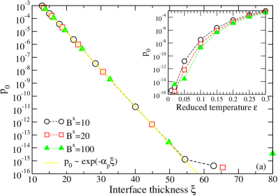
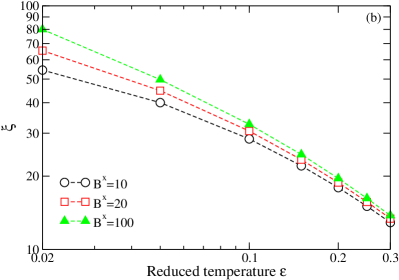
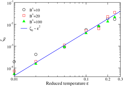
As shown in Fig. 2 (a), the pinning strength $p_{0}$ increases with the decrease of system temperature (i.e., with the increasing value of $\epsilon$; see the inset), and also with the decrease of bulk elastic modulus $B^{x}$ for large enough $p_{0}$ ($>10^{-14}$). This can be attributed to the phenomenon of sharper liquid-solid interface at lower temperature and smaller value of $B^{x}$ [see Fig. 2 (b)], since sharper interface leads to stronger scale coupling between microscopic crystalline structure and mesoscopic amplitudes, and hence larger pinning force; this is a fundamental mechanism underlying the nonadiabatic derivation given in Sec. II. Thus one would expect that there might be a more universal relation between the pinning force and the interface thickness $\xi$, as can be derived from Eq. (33) governing $p_{0}$: Recalling that both amplitudes $A_{j}^{0}$ and $n_{0}^{0}$ are functions of scaled variable $U=u/\xi$ in the inner region (see Sec. III.2), we rewrite Eq. (33) as

$$p_{0}=\left|\int_{-\infty}^{+\infty}due^{iq_{0}u}G(u/\xi)\right|,$$ (51)

where $G=A_{1}^{0}\partial_{u}f_{p_{1}}^{*}+{A_{2}^{0}}^{*}\partial_{u}f_{p_{2}}+A_{3}^{0}\partial_{u}f_{p_{3}}^{*}$. Applying the residue theorem to the integral in Eq. (51) and assuming that within the poles (singularities) of $G(U=u/\xi)$ in the upper-half complex plane, the one nearest to the real axis is given by $U_{z}=u_{z}/\xi=\beta_{s}+i\alpha_{s}$ (i.e., $\alpha_{s}$ is of the smallest value within all poles), we find

$$p_{0}\sim e^{-\alpha_{p}\xi},$$ (52)

where $\alpha_{p}=q_{0}\alpha_{s}>0$. This scaling form is verified in Fig. 2 (a): All the data from different systems characterized by distinct elastic constants (i.e., different $B^{x}$ values) can be scaled onto a single universal curve obeying Eq. (52) (except for very small values of $p_{0}<10^{-14}$ for which numerical errors would be too large), where $\alpha_{p}=0.6620\pm 0.0008$ as determined from data fitting.

Note that numerical results in Fig. 2 (a) seem to imply an asymptotic behavior of $p_{0}\rightarrow 0$ as the system approaches the melting point (i.e., $\epsilon\rightarrow 0$). However, since this is a subcritical bifurcation system (with hexagonal symmetry), the interface thickness $\xi$ remains finite and the pinning strength $p_{0}$ would never vanish as $\epsilon\rightarrow 0$ Boyer and Viñals (2002b) in both real systems and the full PFC model.

Figure 2: (Color online) (a) Pinning strength $p_{0}$ as a function of interface thickness $\xi$ or reduced temperature $\epsilon$ (inset), for different values of elastic modulus $B^{x}$. The result indicates a universal relation given in Eq. (52): $p_{0}\sim\exp(-\alpha_{p}\xi)$, with $\alpha_{p}=0.6620\pm 0.0008$. (b) Change of interface thickness $\xi$ with the reduced temperature $\epsilon$. Note that larger value of $\epsilon$ corresponds to lower system temperature; also for comparison, the numerical value of atomic layer spacing is $a_{0}=2\pi/q_{0}\sim 6.28$.

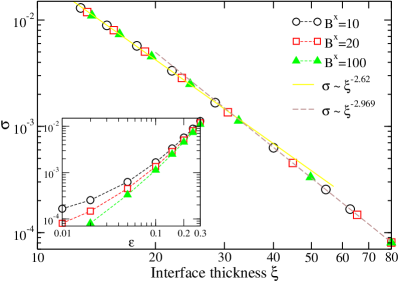
A universal scaling behavior can be also identified for the surface tension $\sigma$, although the form of scaling is different. As shown in Fig. 3 where the results are calculated from Eq. (41), values of $\sigma$ for systems of different elastic modulus $B^{x}$ are well fitted into a single scaling curve of $\sigma$ vs. $\xi$. This data collapse works well for all range of interface thickness $\xi$ in our calculations, yielding a power law behavior $\sigma\sim\xi^{-\alpha_{\sigma}}$, although with two power-law exponents found in two distinct regimes: For thin enough interface $\alpha_{\sigma}=2.62\pm 0.02$, while more diffuse interface results in a faster decay of $\sigma$ determined by $\alpha_{\sigma}=2.969\pm 0.005$. The crossover between these two scaling regimes is identified in Fig. 3. Note that generally surface tension $\sigma$ becomes larger for larger value of $\epsilon$ (lower temperature), and also for sharper interface with smaller $B^{x}$ (see the inset of Fig. 3), as expected.

Figure 3: (Color online) Surface tension $\sigma$ as a function of $\xi$ or $\epsilon$ (inset). All data for different values of $B^{x}$ collapses on a single universal curve of $\sigma$ vs. $\xi$, which can be fitted into 2 power-law relations: $\sigma\sim\xi^{-2.62\pm 0.02}$ for small interface width and $\sigma\sim\xi^{-2.969\pm 0.005}$ for more diffuse interfaces. The crossover occurs at an intermediate width value $\xi\sim 33$.

Another important parameter governing interface motion is the kinetic coefficient $\zeta_{0}$, which determines the relation between the interface velocity and the thermodynamic driving force and is of large interest in solidification studies Mikheev and Chernov (1991); Mendelev et al. (2010); *re:monk10. Note that the expression of $\zeta_{0}$ given in Eq. (46), if neglecting the last average density term, is similar to that determined by Mikheev and Chernov from classical density functional theory Mikheev and Chernov (1991) which can well describe recent results of molecular dynamics simulations Mendelev et al. (2010). The anisotropic feature of kinetic coefficient identified in previous studies has also been incorporated in Eq. (46), as the amplitude profiles ($A_{j}^{0}$ and $n_{0}^{0}$) vary with the orientation of liquid-solid interface.

On the other hand, here we focus on a system different from these previous studies [although the general form of interface equations (44), (49), and (48) is applicable to both cases]: Instead of using interface undercooling as the thermodynamic driving force Mikheev and Chernov (1991); Mendelev et al. (2010); Monk et al. (2010), here we study the isothermal solidification process in pure materials, and the driving force originates from the supersaturation in atomic density at uniform temperature. We can then examine the kinetic coefficient for different isothermal systems, each with a specific $\epsilon$ value and the corresponding liquid-solid coexistence conditions. Results evaluated from Eq. (46) are given in Fig. 4, showing the increase of $\zeta_{0}$ with decreasing temperature (i.e., larger $\epsilon$). Data of different elastic modulus $B^{x}$ fall around a power-law relation $\zeta_{0}\sim\epsilon^{2}$, although with large deviation found at small $B^{x}$ and $\epsilon$ values (i.e., $B^{x}=10$ and $\epsilon\leq 0.02$).

Figure 4: (Color online) Kinetic coefficient $\zeta_{0}$ as a function of reduced temperature $\epsilon$, for different values of $B^{x}$. An estimate of $\zeta_{0}\sim\epsilon^{2}$ is shown for comparison. Note that the thermodynamic driving force here is not interface undercooling, but the density supersaturation in isothermal systems.

IV.2 Planar interface dynamics and pinning

In the case of planar growth along the normal $y$ direction, the lateral variations in the interface equations of motion can be neglected, resulting in an effective 1D system. In the frame co-moving with the interface at a velocity $v_{0}$, the outer equation (49) in the liquid region ($y>0$, and $y\rightarrow y-v_{0}t$) leads to a steady-state form

$$v_{0}\partial_{y}\delta n_{0}+\left(q_{0}^{4}+\beta_{0}\right)\partial_{y}^{2}\delta n_{0}=0,$$ (53)

where $\beta_{0}=-\epsilon+3{n_{0}^{0}}^{2}(+\infty)-2gn_{0}^{0}(+\infty)$. The liquid-state chemical potential variation is given by $\delta\mu(y>0)=(q_{0}^{4}+\beta_{0})\delta n_{0}$, satisfying a far-field boundary condition $\delta\mu(+\infty)=\Delta$ which represents an external growth condition of constant flux coming from the liquid boundary. In the solid side ($y<0$), the outer solution yields a constant $\delta\mu(y<0)=\delta\mu(0)$. From the interface condition $v_{0}\Delta n_{0}^{0}=-\partial_{y}\delta\mu|_{0^{+}}$ as determined by Eq. (48) and the continuity of $\delta\mu$, we obtain the steady-state solution

$$\delta\mu=\left\{\begin{array}[]{l}\delta\mu_{0}\exp\left(-\frac{v_{0}}{q_{0}^{4}+\beta_{0}}y\right)+\Delta,\quad y\geq 0\\ \delta\mu_{0}+\Delta,\quad y\leq 0,\end{array}\right.$$ (54)

where $\delta\mu_{0}=(q_{0}^{4}+\beta_{0})\Delta n_{0}^{0}$. Thus from Eq. (45) the effective driving force is given by

$$F_{0}=\lambda=-q_{0}^{2}\Delta n_{0}^{0}(\delta\mu_{0}+\Delta).$$ (55)

If neglecting the lattice pinning effect, the dynamics of interface profile is trivial: $h(t)=h(0)+v_{0}t$, with a constant interface growth rate $v_{0}=F_{0}/\zeta_{0}=-q_{0}^{2}\Delta n_{0}^{0}(\delta\mu_{0}+\Delta)/\zeta_{0}$. However, as will be shown below the lattice coupling effect plays a significant role in the description of interface dynamics, even for the simplest case of layer-by-layer growth considered here.

The dynamical equation governing a planar interface profile $h(t)$ is derived from Eq. (50), i.e.,

$$\zeta_{0}v_{n}=\zeta_{0}\partial h/\partial t=F_{0}-p_{0}\sin(q_{0}h+\varphi)+\eta_{v},$$ (56)

which can be solved exactly in the absence of the noise term $\eta_{v}$, as given in the following.

Figure 5: (Color online) Propagation of interface position $h$ with time $t$, as evaluated from analytic solutions (57) for $|F_{0}|=1.1p_{0}$ and (59) for $|F_{0}|=0.9p_{0}$, with $\epsilon=0.3$ and $B^{x}=10$. Positions of $h$ are shown in unit of atomic layer spacing $a_{0}=2\pi/q_{0}$.

IV.2.1 $|F_{0}|>p_{0}$: continuous growth mode

When the magnitude of external driving force exceeds the lattice pinning strength $p_{0}$, the exact solution of the interface position is written as

$$h(t)= \pm\frac{2}{q_{0}}\arctan\left\{\beta\tan\left[\frac{q_{0}}{2\zeta_{0}}\left(F_{0}^{2}-p_{0}^{2}\right)^{1/2}t\pm\tau_{0}\right]\right\}$$ (57)

$$-\left(\varphi-\frac{\pi}{2}\right)/q_{0}$$

with “$+$” for $F_{0}>0$ and “$-$” for $F_{0}<0$, where $\beta=[(F_{0}-p_{0})/(F_{0}+p_{0})]^{1/2}$ and $\tau_{0}$ is determined by initial condition, i.e.,

$$\tau_{0}=\arctan\left\{\frac{1}{\beta}\tan\left[\frac{q_{0}}{2}h(0)+\frac{\varphi}{2}-\frac{\pi}{4}\right]\right\}.$$ (58)

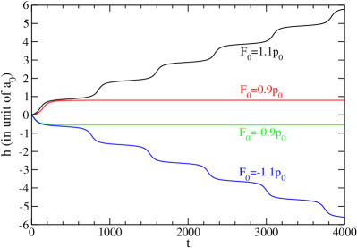
This situation could occur at small enough $\epsilon$ (i.e., high temperature growth) and diffuse enough interface, and hence small enough pinning force (see Fig. 2), given a certain flux condition $F_{0}$. Despite its form of continuum description, the solution (57) yields the jumps of distance $2\pi/q_{0}$ ($=a_{0}$) for interface position, which is exactly one discrete lattice spacing along the $y$ direction of growth. As shown in Fig. 5 which gives the numerical evaluation of Eq. (57), the liquid-solid interface propagates “continuously” due to the overcoming of lattice pinning, while the discrete lattice effect can still be preserved in this continuous growth mode as a form of growing steps of $a_{0}$ spacing. In this case the average velocity of interface can be calculated as $\bar{v}=\langle dh/dt\rangle=\pm(F_{0}^{2}-p_{0}^{2})^{1/2}/\zeta_{0}$.

IV.2.2 $|F_{0}|<p_{0}$: activated/nucleated growth mode

For the growth condition of lower temperature and sharper interface (with larger pinning strength) or weaker driving force such that $|F_{0}|<p_{0}$, the exact solution of Eq. (56) without noise is different:

$$h(t)=\frac{2}{q_{0}}\arctan\left[\beta^{\prime}\frac{1+\tau_{0}^{\prime}f_{0}(t)}{1-\tau_{0}^{\prime}f_{0}(t)}\right]-\left(\varphi-\frac{\pi}{2}\right)/q_{0},$$ (59)

where $\beta^{\prime}=[(p_{0}-F_{0})/(p_{0}+F_{0})]^{1/2}$, $f_{0}(t)=\exp[q_{0}(p_{0}^{2}-F_{0}^{2})^{1/2}t/\zeta_{0}]$, and

$$\tau_{0}^{\prime}=\frac{\tan\left[\frac{q_{0}}{2}h(0)+\frac{\varphi}{2}-\frac{\pi}{4}\right]-\beta^{\prime}}{\tan\left[\frac{q_{0}}{2}h(0)+\frac{\varphi}{2}-\frac{\pi}{4}\right]+\beta^{\prime}}.$$ (60)

The interface growth rate is then given by

$$v_{n}=dh/dt=\frac{(4/\zeta_{0})(p_{0}-F_{0})\tau_{0}^{\prime}f_{0}(t)}{\left[1-\tau_{0}^{\prime}f_{0}(t)\right]^{2}+\beta^{\prime 2}\left[1+\tau_{0}^{\prime}f_{0}(t)\right]^{2}}.$$ (61)

At large time $t\gg 1$, $v_{n}=dh/dt\rightarrow 0$; the interface is thus locked/pinned by the underlying crystalline potential at a position $h=-(2\arctan\beta^{\prime}+\varphi-\pi/2)/q_{0}$ (satisfying $\sin(q_{0}h+\varphi)=F_{0}/p_{0}$). This pinning phenomenon is illustrated in Fig. 5 which shows the numerical evaluation of the analytic solution (59).

Thermal fluctuations should then play an important role on the process of lattice growth and interface moving, and the full stochastic dynamic equation (56) with noise term $\eta_{v}$ governed by Eq. (47) should be used. This will become a stochastic, escape problem in a potential system Boyer and Viñals (2002a), and the liquid-solid front would propagate via an activated process to overcome the pinned lattice site, a procedure analogous to thermal nucleation. To illustrate this depinning process, we rewrite Eq. (56) as

$$dh/dt=-\frac{\partial U_{h}}{\partial h}+\eta_{h},$$ (62)

where the effective potential $U_{h}=-[(p_{0}/q_{0})\cos(q_{0}h+\varphi)+F_{0}h]/\zeta_{0}$ and the noise $\eta_{h}$ satisfies $\langle\eta_{h}(t)\eta_{h}(t^{\prime})\rangle=2D_{0}\delta(t-t^{\prime})$, with $D_{0}=D/\zeta_{0}^{2}=\vartheta q_{0}^{2}\Gamma_{0}k_{B}T/\zeta_{0}$. From the corresponding Fokker-Planck equation we can determine the Kramers’ escape rate

$$R=\frac{1}{\tau}=\frac{1}{2\pi}\left[\left.\frac{\partial^{2}U_{h}}{\partial h^{2}}\right|_{a}\left|\frac{\partial^{2}U_{h}}{\partial h^{2}}\right|_{b}\right]^{2}e^{-\Delta U_{h}/D_{0}},$$ (63)

which represents the rate of an atom hopping/escaping from a metastable lattice site “$a$” (determined as a local minimum of potential $U_{h}$) to a nearest lattice site with lower potential, via overcoming a potential barrier $\Delta U_{h}=U_{h}(b)-U_{h}(a)$ where “$b$” indicates the top location of the barrier (i.e., a local maximum of $U_{h}$). In Eq. (63) $\tau$ is the escape time of atoms. It can be shown that $\partial^{2}U_{h}/\partial h^{2}|_{a}=-\partial^{2}U_{h}/\partial h^{2}|_{b}=q_{0}(p_{0}^{2}-F_{0}^{2})^{1/2}/\zeta_{0}$, and the potential barrier

$$\Delta U_{h}=\frac{2}{q_{0}\zeta_{0}}\left[\left(p_{0}^{2}-F_{0}^{2}\right)^{1/2}-|F_{0}|\arccos\left(|F_{0}|/p_{0}\right)\right]$$ (64)

(which is always positive for $|F_{0}|<p_{0}$).

In this thermally activated process, the lattice nucleation growth rate is given by $I=a_{0}R=a_{0}/\tau$, where $a_{0}=2\pi/q_{0}$ is the spacing of atomic layers along the growth direction $\hat{y}$ as shown in Fig. 1 and Sec. II. From Eqs. (63), (64) and the expression of $D_{0}$, we obtain the standard Arrhenius form for thermal nucleation:

$$I=I_{0}e^{-E_{a}/k_{B}T},$$ (65)

where

$$I_{0}=(p_{0}^{2}-F_{0}^{2})^{1/2}/\zeta_{0},$$ (66)

and the activation energy $E_{a}$ is determined by

$$E_{a}=\frac{2}{\vartheta q_{0}^{3}\Gamma_{0}}\left[\left(p_{0}^{2}-F_{0}^{2}\right)^{1/2}-|F_{0}|\arccos\left(|F_{0}|/p_{0}\right)\right].$$ (67)

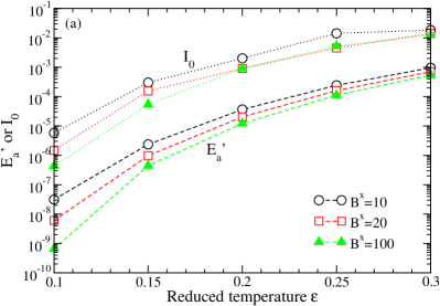
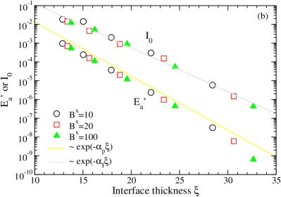
It is important to note that in the general form of Eq. (65), both the prefactor $I_{0}$ and activation energy $E_{a}$ are actually dependent on temperature ($\epsilon$) and also elastic constants ($B^{x}$), as can be seen from their expressions in Eqs. (66) and (67). For a simple example, if setting a growth condition of $F_{0}=\alpha_{0}p_{0}$ ($|\alpha_{0}|<1$) for all temperatures or $\epsilon$ values, we have the rescaled activation energy $E_{a}^{\prime}=E_{a}\vartheta\Gamma_{0}=(2/q_{0}^{3})[(1-\alpha_{0}^{2})^{1/2}-|\alpha_{0}|\arccos|\alpha_{0}|]p_{0}$, showing the same behavior of temperature and interface width dependence as that of $p_{0}$ (see Fig. 2). On the other hand, considering constant driving force $F_{0}$ at different temperatures would lead to more complicated temperature and width dependence of $E_{a}$ and $I_{0}$, as shown in Fig. 6. The results there are obtained from numerical evaluations of Eqs. (67) and (66). Fig. 6 (a) shows that both $E_{a}^{\prime}$ and $I_{0}$ increase with $\epsilon$ (i.e., the decrease of temperature). At low temperatures with large $\epsilon$ and small interface thickness $\xi$, $p_{0}\gg F_{0}$ and Eq. (67) yields $E_{a}^{\prime}\propto p_{0}$. We would then expect the activation energy to follow a universal scaling relation similar to that of pinning strength $p_{0}$: $E_{a}^{\prime}\sim\exp(-\alpha_{p}\xi)$. A deviation would occur for large enough $\xi$ (i.e., small enough $\epsilon$ and high enough temperature) due to similar order of magnitudes between $p_{0}$ and $F_{0}$ values, as has been verified in Fig. 6 (b). Also interestingly, all the numerical data of prefactor $I_{0}$ for different values of elastic modulus ($B^{x}$) is found to collapse on a universal curve $I_{0}\sim\exp(-\alpha_{I}\xi)$, where $\alpha_{I}=0.54\pm 0.01$ as obtained from data fitting. All these results indicate that in the PFC model the temperature dependence of nucleation rate $I$ is not exactly Arrhenius, but shows a more complicated nonlinear behavior.

Figure 6: (Color online) The rescaled activation energy $E_{a}^{\prime}=E_{a}\vartheta\Gamma_{0}$ and the prefactor $I_{0}$ of the nucleation growth rate as a function of (a) reduced temperature $\epsilon$ and (b) interface width $\xi$, for different values of $B^{x}$ and a constant $F_{0}=10^{-9}$. In (b), all data of $I_{0}$ are fitted into a scaling form $I_{0}\sim\exp(-\alpha_{I}\xi)$, where $\alpha_{I}=0.54\pm 0.01$; for the data of $E_{a}^{\prime}$, the scaling relation of $p_{0}$ [$\sim\exp(-\alpha_{p}\xi)$] is shown for comparison.

V Discussion and Conclusions

We have constructed a nonadiabatic amplitude representation and examined the sharp-interface limit of the 2D single-component PFC model. Our main findings include the coupling and interaction between mesoscopic description (for “slow” variation of structural amplitudes) and microscopic scales (for “fast” variation of the underlying crystalline structure), and also the resulting interface pinning effects which are incorporated in a generalized Gibbs-Thomson relation for interface dynamics. The strength of the corresponding pinning force, and also the value of solid surface tension, have been found to obey universal scaling relations with respect to the liquid-solid interface width. Temperature dependence of the interface kinetic coefficient has also been examined for isothermal systems driven by density supersaturation. The scale coupling effects have been illustrated in an example of planar interface growth, which shows the crossover between two distinct growth modes, a “continuous” or nonactivated mode for high-temperature or strongly-driven growth and a “nucleated” mode for low/moderate temperature or weakly-driven growth, as a result of the competition between the external thermodynamic driving force and the lattice pinning/locking effect. Such thermal nucleation process in the growth regime of $|F_{0}|<p_{0}$ is analogous to a pinning-depinning transition in the absence of quenched disorder.

Note that the sample application given in Sec. IV.2 can be viewed as the lowest order approximation of interface growth, and the scenario of nonactivated/continuous vs. activated growth modes identified is qualitatively consistent with the classical crystal growth theory of Cahn Cahn (1960) based on the concept of critical driving force, and also with that found in early work of roughening transition by Chui and Weeks Chui and Weeks (1978) and Nozières and Gallet Nozières and Gallet (1987), although more complicated parameter dependence on temperature and material elastic property is determined here. More general study should involve nonplanar surface/interface evolution and dynamics, so that details of dynamic roughening and faceting transition involving this new parameter dependence can be obtained. Also, all the above derivations can be readily extended to (2+1)D PFC growth systems with 3D bcc or fcc lattice structure. The corresponding interface equations are expected to be of the same form as Eqs. (48), (49), and the generalized Gibbs-Thomson relation (44); the latter could be also reduced to a driven sine-Gordon form (i.e., the form of the (2+1)D Hwa-Kardar-Paczuski equation Hwa et al. (1991)) governing the interface profile $h(\bm{r},t)$:

$$\zeta_{0}\partial h/\partial t=F_{0}+\sigma\nabla^{2}h+\frac{\lambda}{2}\left|\bm{\nabla}h\right|^{2}-p_{0}\sin(q_{0}h+\varphi)+\eta_{v},$$ (68)

although with more complicated expression of the coefficients. It is important to note that generally $F_{0}$ and $\lambda$ are functions of $h$ and lateral coordinate $\bm{r}$ in both (1+1)D and (2+1)D cases, as can be seen from $\delta\mu(0,s)=\delta\mu(y=h,x)$ in Eq. (45). Thus the above driven sine-Gordon form is actually a much more complex nonlinear equation of $h$, and is closely coupled to the conservation condition (48) and the outer equation (49) which reflect the conserved dynamics of atomic number density. On the other hand, if neglecting the spatial dependence of $F_{0}$ and $\lambda$ at lowest order approximation [i.e., approximating $F_{0}$ and $\lambda$ by the planar constant result Eq. (55) for the case of weak surface fluctuations], the Hwa-Kardar-Paczuski equation with spatially-constant coefficients can be recovered. In further studies it would be interesting to identify the properties of the corresponding dynamic roughening transition as compared to the previous renormalization-group results Nozières and Gallet (1987); Hwa et al. (1991) (noting that from our derivation coefficients in Eq. (68) are generally temperature dependent), although one would expect such transition to be near the lowest order result of $|F_{0}|=p_{0}$.

Another important topic to be addressed, based on the nonadiabatic amplitude representation and sharp-interface approach developed here, is the anisotropy along different crystal growth directions, particularly for surface tension ($\sigma$), kinetic coefficient ($\zeta_{0}$), and pinning strength ($p_{0}$). This would yield detailed properties of facet formation and anisotropic, orientation-dependent roughening transition. Note that all the results given in Sec. III and IV are for interfaces oriented along the $y$ direction. For other orientations we expect the same forms of interface equations of motion due to similar derivation procedure, but with different values/expressions of coefficients. For example, as shown explicitly in Eqs. (11)–(14) and Fig. 1, atomic layers oriented along $\hat{y}$ or $(\pm\sqrt{3}\hat{x}+\hat{y})/2$ direction are not equivalent to those along $\hat{x}$ or $(\pm\hat{x}+\sqrt{3}\hat{y})/2$ direction, due to different layer spacing ($a_{0}$ vs. $a_{0}/\sqrt{3}$) and hence different degree of scale coupling and pinning effect. Similar properties are expected for 3D PFC models of various symmetries, although with more complicated results anticipated.

Appendix A Derivation of lattice pinning term in the interface equation of motion

To derive the interface equation from the nonconserved dynamic equations for $A_{j}$, we perform integration of $\int_{-\bar{\zeta}}^{\bar{\zeta}}dU\partial_{U}{A_{j}^{0}}^{*}$ on Eq. (28) and also summation over all the resulting equations for $A_{j}$ and $A_{j}^{*}$. Corresponding to the last scale-coupling term in Eq. (28), we get

$$-\frac{1}{\bar{\lambda}_{y}}\sum_{j}\int_{-\bar{\zeta}}^{\bar{\zeta}}dU\left[\left(\partial_{U}{A_{j}^{0}}^{*}\right)\int_{U}^{U+\bar{\lambda}_{y}}dU^{\prime}f_{p_{j}}(A_{j}^{0},n_{0}^{0})~{}e^{\mp i\bar{q}_{0}(U^{\prime}+\tilde{h})}+\text{c.c.}\right]$$

$$=-\frac{e^{i\bar{q}_{0}\tilde{h}}}{\bar{\lambda}_{y}}\left[\int dA_{1}^{0}\int_{U}^{U+\bar{\lambda}_{y}}dU^{\prime}f_{p_{1}}^{*}~{}e^{i\bar{q}_{0}U^{\prime}}+\int d{A_{2}^{0}}^{*}\int_{U}^{U+\bar{\lambda}_{y}}dU^{\prime}f_{p_{2}}~{}e^{i\bar{q}_{0}U^{\prime}}+\int dA_{3}^{0}\int_{U}^{U+\bar{\lambda}_{y}}dU^{\prime}f_{p_{3}}^{*}~{}e^{i\bar{q}_{0}U^{\prime}}\right]+\text{c.c.}$$

$$=\frac{e^{i\bar{q}_{0}\tilde{h}}}{\bar{\lambda}_{y}}\left\{\int dUA_{1}^{0}e^{i\bar{q}_{0}U}\left[f_{p_{1}}^{*}(U+\bar{\lambda}_{y})-f_{p_{1}}^{*}(U)\right]+\int dU{A_{2}^{0}}^{*}e^{i\bar{q}_{0}U}\left[f_{p_{2}}(U+\bar{\lambda}_{y})-f_{p_{2}}(U)\right]\right.$$

$$\left.\quad+\int dUA_{3}^{0}e^{i\bar{q}_{0}U}\left[f_{p_{3}}^{*}(U+\bar{\lambda}_{y})-f_{p_{3}}^{*}(U)\right]\right\}+\text{c.c.}$$

$$\simeq e^{i\bar{q}_{0}\tilde{h}}\int dU~{}e^{i\bar{q}_{0}U}\left[A_{1}^{0}\partial_{U}f_{p_{1}}^{*}+{A_{2}^{0}}^{*}\partial_{U}f_{p_{2}}+A_{3}^{0}\partial_{U}f_{p_{3}}^{*}\right]+\text{c.c.},$$ (69)

where $f_{p_{j}}(U)\equiv f_{p_{j}}(A_{j}^{0}(U),n_{0}^{0}(U))$, and we have used $\bar{q}_{0}\bar{\lambda}_{y}=4\pi$ and $[f_{p_{j}}(U+\bar{\lambda}_{y})-f_{p_{j}}(U)]/\bar{\lambda}_{y}\simeq\partial_{U}f_{p_{j}}$. It is then straightforward to show that (69) is equivalent to the lattice pinning term $p_{0}\sin(\bar{q}_{0}\tilde{h}+\varphi)$ appearing in Eq. (31), with the pinning strength $p_{0}$ and phase $\varphi$ determined by Eq. (33).

Appendix B Matching between inner and outer regions and the Gibbs surface condition

In the inner region, the solution of Eq. (34) for Green’s functions $G^{\pm}$ satisfying the corresponding boundary conditions at $U,U^{\prime}=0,\pm\bar{\zeta}$ has been given in Ref. Elder et al. (2001), i.e.,

$$G^{+}(U,S;U^{\prime},S^{\prime})=\left\{\begin{array}[]{l}-U^{\prime}\delta(S-S^{\prime}),\quad 0\leq U^{\prime}<U\leq\bar{\zeta}\\ -U\delta(S-S^{\prime}),\quad~{}0\leq U<U^{\prime}\leq\bar{\zeta}\end{array}\right.$$ (72)

$$G^{-}(U,S;U^{\prime},S^{\prime})=\left\{\begin{array}[]{l}U\delta(S-S^{\prime}),\quad-\bar{\zeta}\leq U^{\prime}<U\leq 0\\ U^{\prime}\delta(S-S^{\prime}),\quad-\bar{\zeta}\leq U<U^{\prime}\leq 0.\end{array}\right.$$ (75)

(76)

Substituting solution (76) into Eq. (35) leads to

$$-\tilde{v}(S)\xi^{2} \int_{0^{+}}^{U}dU^{\prime}[n_{0}^{0}-n_{0}^{0}(+\bar{\zeta})]=\tilde{\mu}_{1}(U,S)-\tilde{\mu}_{1}(0^{+},S)$$ (77)

$$-U\left(\partial_{U}\tilde{\mu}_{1}\right)_{\bar{\zeta}}+\xi\int_{0^{+}}^{U}dU^{\prime}[\tilde{\eta}_{0}^{u}-\tilde{\eta}_{0}^{u}(+\bar{\zeta})],$$

$$-\tilde{v}(S)\xi^{2} \int_{0^{-}}^{U}dU^{\prime}[n_{0}^{0}-n_{0}^{0}(-\bar{\zeta})]=\tilde{\mu}_{1}(U,S)-\tilde{\mu}_{1}(0^{-},S)$$ (78)

$$-U\left(\partial_{U}\tilde{\mu}_{1}\right)_{-\bar{\zeta}}+\xi\int_{0^{-}}^{U}dU^{\prime}[\tilde{\eta}_{0}^{u}-\tilde{\eta}_{0}^{u}(-\bar{\zeta})],$$

where Eq. (77) applies to $0^{+}\leq U\leq\bar{\zeta}$ and (78) applies to $-\bar{\zeta}\leq U\leq 0^{-}$.

From the rescaling $(U,S)=(u/\xi,\varepsilon s/\xi)$ in the inner region and $(U^{o},S^{o})=(\varepsilon u/\xi,\varepsilon s/\xi)$ for the outer region, the matching conditions (43) can be rewritten as

$$\tilde{\mu}_{1}(U=\pm\bar{\zeta},S)=\tilde{\mu}_{1}^{\text{out}}(U^{o}=\pm\varepsilon\bar{\zeta},S^{o}),$$

$$\left(\partial_{U}\tilde{\mu}_{1}\right)_{U=\pm\bar{\zeta}}=\varepsilon\left(\partial_{U^{o}}\tilde{\mu}_{1}^{\text{out}}\right)_{U^{o}=\pm\varepsilon\bar{\zeta}}.$$ (79)

Also, due to $\varepsilon\bar{\zeta}=\varepsilon\zeta/\xi\ll 1$ we can carry out the expansion for the outer solution

$$\tilde{\mu}_{1}^{\text{out}}(0^{\pm},S^{o})=\tilde{\mu}_{1}^{\text{out}}(\pm\varepsilon\bar{\zeta},S^{o})\mp\varepsilon\bar{\zeta}\left(\partial_{U^{o}}\tilde{\mu}_{1}^{\text{out}}\right)_{\pm\varepsilon\bar{\zeta}}+\mathcal{O}(\varepsilon^{2}).$$ (80)

Evaluating Eq. (77) with $U=+\bar{\zeta}$ and Eq. (78) with $U=-\bar{\zeta}$, and using conditions (79) and (80), we find

$$-\tilde{v}\xi^{2}\int_{0}^{\bar{\zeta}}dU^{\prime} [n_{0}^{0}-n_{0}^{0}(+\bar{\zeta})]=\tilde{\mu}_{1}^{\text{out}}(0^{+},S^{o})-\tilde{\mu}_{1}(0^{+},S)$$ (81)

$$+\xi\int_{0}^{\bar{\zeta}}dU^{\prime}[\tilde{\eta}_{0}^{u}-\tilde{\eta}_{0}^{u}(+\bar{\zeta})]+\mathcal{O}(\varepsilon^{2}),$$

$$\tilde{v}\xi^{2}\int_{-\bar{\zeta}}^{0}dU^{\prime} [n_{0}^{0}-n_{0}^{0}(-\bar{\zeta})]=\tilde{\mu}_{1}^{\text{out}}(0^{-},S^{o})-\tilde{\mu}_{1}(0^{-},S)$$ (82)

$$-\xi\int_{-\bar{\zeta}}^{0}dU^{\prime}[\tilde{\eta}_{0}^{u}-\tilde{\eta}_{0}^{u}(-\bar{\zeta})]+\mathcal{O}(\varepsilon^{2}).$$

Adding Eqs. (81) and (82), using the Gibbs surface condition (42), and considering $\bar{\zeta}=\zeta/\xi\gg 1$, we get

$$\tilde{\mu}_{1}(0,S)=\tilde{\mu}_{1}^{\text{out}}(0,S^{o})+\tilde{v}\xi^{2}\int_{0}^{\infty}dU[n_{0}^{0}-n_{0}^{0}(+\infty)]+\tilde{\eta}_{m},$$ (83)

where $\tilde{\eta}_{m}=\eta_{m}/\varepsilon=\{\int_{0}^{\infty}du[\tilde{\eta}_{0}^{u}-\tilde{\eta}_{0}^{u}(+\infty)]-\int_{-\infty}^{0}du[\tilde{\eta}_{0}^{u}-\tilde{\eta}_{0}^{u}(-\infty)]\}/2$ (with $\tilde{\eta}_{0}^{u}=\eta_{0}^{u}/\varepsilon$). Rewriting Eq. (83) in the original scale $(u,s)$ and substituting into the interface equation (40), we can obtain the generalized Gibbs-Thomson relation given in Eq. (44).

To derive the standard interface continuity condition (48), we apply the matching condition (79) to Eq. (39) and expand the outer result around $u=0$; that is, $(\partial_{U}\tilde{\mu}_{1})_{\pm\bar{\zeta}}=\varepsilon(\partial_{U^{o}}\tilde{\mu}_{1}^{\text{out}})_{\pm\varepsilon\bar{\zeta}}=\varepsilon(\partial_{U^{o}}\tilde{\mu}_{1}^{\text{out}})_{0^{\pm}}\pm\varepsilon^{2}\bar{\zeta}(\partial_{U^{o}}^{2}\tilde{\mu}_{1}^{\text{out}})_{0^{\pm}}+\mathcal{O}(\varepsilon^{3})$. Keeping terms up to $\mathcal{O}(\varepsilon)$ and neglecting the noise effect in the outer solution would then yield Eq. (48) in the original scale.

Note that the Gibbs surface condition can actually be determined from Eqs. (81) and (82) up to $\mathcal{O}(\varepsilon)$. Subtracting Eq. (81) from (82) and neglecting the noise terms, given the continuity of $\tilde{\mu}_{1}$ and $\tilde{\mu}_{1}^{\text{out}}$ at $u=0^{\pm}$ we obtain

$$\int_{-\bar{\zeta}}^{\bar{\zeta}}dU\left[n_{0}^{0}-n_{0}^{0}(\pm\bar{\zeta})\right]\simeq\mathcal{O}(\varepsilon^{2}).$$ (84)

Returning to the original scale and noting $\bar{\zeta}\gg 1$, at $\mathcal{O}(\varepsilon)$ we can recover Eq. (42) for the Gibbs surface.

References

- Langer (1980) J. S. Langer, Rev. Mod. Phys. 52, 1 (1980).
- Elder et al. (1994) K. R. Elder, F. Drolet, J. M. Kosterlitz, and M. Grant, Phys. Rev. Lett. 72, 677 (1994).
- Karma and Rappel (1998) A. Karma and W.-J. Rappel, Phys. Rev. E 57, 4323 (1998).
- Elder et al. (2001) K. R. Elder, M. Grant, N. Provatas, and J. M. Kosterlitz, Phys. Rev. E 64, 021604 (2001).
- Müller and Grant (1999) J. Müller and M. Grant, Phys. Rev. Lett. 82, 1736 (1999).
- Kassner et al. (2001) K. Kassner, C. Misbah, J. Müller, J. Kappey, and P. Kohlert, Phys. Rev. E 63, 036117 (2001).
- Granasy et al. (2004) L. Granasy, T. Pusztai, T. Borzsonyi, J. A. Warren, and J. F. Douglas, Nature Mater. 3, 645 (2004).
- Wang and Li (2010) Y. Wang and J. Li, Acta Mater. 58, 1212 (2010).
- Chui and Weeks (1978) S. T. Chui and J. D. Weeks, Phys. Rev. Lett. 40, 733 (1978).
- Nozières and Gallet (1987) P. Nozières and F. Gallet, J. Physique 48, 353 (1987).
- Hwa et al. (1991) T. Hwa, M. Kardar, and M. Paczuski, Phys. Rev. Lett. 66, 441 (1991).
- Balibar and Bouchaud (1992) S. Balibar and J. P. Bouchaud, Phys. Rev. Lett. 69, 862 (1992).
- Mikheev (1993) L. V. Mikheev, Phys. Rev. Lett. 71, 2347 (1993).
- Rost and Spohn (1994) M. Rost and H. Spohn, Phys. Rev. Lett. 72, 784 (1994).
- Hwa et al. (1994) T. Hwa, M. Kardar, and M. Paczuski, Phys. Rev. Lett. 72, 785 (1994).
- Elder et al. (2002) K. R. Elder, M. Katakowski, M. Haataja, and M. Grant, Phys. Rev. Lett. 88, 245701 (2002).
- Elder and Grant (2004) K. R. Elder and M. Grant, Phys. Rev. E 70, 051605 (2004).
- Elder et al. (2007) K. R. Elder, N. Provatas, J. Berry, P. Stefanovic, and M. Grant, Phys. Rev. B 75, 064107 (2007).
- Huang et al. (2010) Z.-F. Huang, K. R. Elder, and N. Provatas, Phys. Rev. E 82, 021605 (2010).
- Greenwood et al. (2010) M. Greenwood, N. Provatas, and J. Rottler, Phys. Rev. Lett. 105, 045702 (2010).
- Greenwood et al. (2011) M. Greenwood, N. Ofori-Opoku, J. Rottler, and N. Provatas, Phys. Rev. B 84, 064104 (2011).
- van Teeffelen et al. (2009) S. van Teeffelen, R. Backofen, A. Voigt, and H. Löwen, Phys. Rev. E 79, 051404 (2009).
- Jaatinen et al. (2009) A. Jaatinen, C. V. Achim, K. R. Elder, and T. Ala-Nissila, Phys. Rev. E 80, 031602 (2009).
- Huang and Elder (2008) Z.-F. Huang and K. R. Elder, Phys. Rev. Lett. 101, 158701 (2008).
- Huang and Elder (2010) Z.-F. Huang and K. R. Elder, Phys. Rev. B 81, 165421 (2010).
- Wu and Voorhees (2009) K.-A. Wu and P. W. Voorhees, Phys. Rev. B 80, 125408 (2009).
- Spatschek and Karma (2010) R. Spatschek and A. Karma, Phys. Rev. B 81, 214201 (2010).
- Muralidharan and Haataja (2010) S. Muralidharan and M. Haataja, Phys. Rev. Lett. 105, 126101 (2010).
- Berry and Grant (2011) J. Berry and M. Grant, Phys. Rev. Lett. 106, 175702 (2011).
- Elder et al. (2012) K. R. Elder, G. Rossi, P. Kanerva, F. Sanches, S.-C. Ying, E. Granato, C. V. Achim, and T. Ala-Nissila, Phys. Rev. Lett. 108, 226102 (2012).
- Wittkowski et al. (2011) R. Wittkowski, H. Löwen, and H. R. Brand, Phys. Rev. E 83, 061706 (2011).
- Goldenfeld et al. (2005) N. Goldenfeld, B. P. Athreya, and J. A. Dantzig, Phys. Rev. E 72, 020601(R) (2005).
- Athreya et al. (2006) B. P. Athreya, N. Goldenfeld, and J. A. Dantzig, Phys. Rev. E 74, 011601 (2006).
- Yeon et al. (2010) D. H. Yeon, Z.-F. Huang, K. R. Elder, and K. Thornton, Phil. Mag. 90, 237 (2010).
- Elder et al. (2010) K. R. Elder, Z.-F. Huang, and N. Provatas, Phys. Rev. E 81, 011602 (2010).
- Pomeau (1986) Y. Pomeau, Physica D 23, 3 (1986).
- Bensimon et al. (1988) D. Bensimon, B. I. Shraiman, and V. Croquette, Phys. Rev. A 38, 5461 (1988).
- Boyer and Viñals (2002a) D. Boyer and J. Viñals, Phys. Rev. E 65, 046119 (2002a).
- Boyer and Viñals (2002b) D. Boyer and J. Viñals, Phys. Rev. Lett. 89, 055501 (2002b).
- Manneville (1990) P. Manneville, Dissipative Structures and Weak Turbulence (Academic, New York, 1990).
- Cross and Hohenberg (1993) M. C. Cross and P. C. Hohenberg, Rev. Mod. Phys. 65, 851 (1993).
- Kardar et al. (1986) M. Kardar, G. Parisi, and Y.-C. Zhang, Phys. Rev. Lett. 56, 889 (1986).
- Mikheev and Chernov (1991) L. V. Mikheev and A. A. Chernov, J. Cryst. Growth 112, 591 (1991).
- Mendelev et al. (2010) M. I. Mendelev, M. J. Rahman, J. J. Hoyt, and M. Asta, Modelling Simul. Mater. Sci. Eng. 18, 074002 (2010).
- Monk et al. (2010) J. Monk, Y. Yang, M. I. Mendelev, M. Asta, J. J. Hoyt, and D. Y. Sun, Modelling Simul. Mater. Sci. Eng. 18, 015004 (2010).
- Cahn (1960) J. W. Cahn, Acta Metall. 8, 554 (1960).