Approximation of Random Slow Manifolds and Settling of Inertial Particles under Uncertainty

Abstract

A method is provided for approximating random slow manifolds of a class of slow-fast stochastic dynamical systems. Thus approximate, low dimensional, reduced slow systems are obtained analytically in the case of sufficiently large time scale separation. To illustrate this dimension reduction procedure, the impact of random environmental fluctuations on the settling motion of inertial particles in a cellular flow field is examined. It is found that noise delays settling for some particles but enhances settling for others. A deterministic stable manifold is an agent to facilitate this phenomenon. Overall, noise appears to delay the settling in an averaged sense.

Key Words: Random slow manifolds, dimension reduction, stochastic differential equations (SDEs), approximation under big scale-separation, inertial particles in flows

Mathematics Subject Classifications (2010): 37H10, 37M99, 60H10

1 Introduction

Complex dynamical systems in science and engineering often involve multiple time scales, such as slow and fast time scales, as well as uncertainty caused by noisy fluctuations. For example, aerosol and pollutant particles, occur in various natural contexts (e.g., in atmosphere and ocean coasts [2, 4, 8]) and engineering systems (e.g. spray droplets), are described by coupled system of differential equations. Some particles move fast while others move slower, and they are usually subject to random influences, due to molecular diffusion, environmental fluctuations, or other small scale mechanisms that are not explicitly modeled [13]. Invariant manifolds are geometric structures in state space that help describe dynamical behaviors of dynamical systems. A slow manifold is a special invariant manifold, with an exponential attracting property and with the dimension the same as the number of slow variables. The reduced system on a slow manifold thus characterizes the long time dynamics in a lower dimensional setting, facilitating geometric and numerical investigation.

Existence for slow manifolds of stochastic dynamical systems with slow-fast time scales has been investigated recently [12, 7]. However, stochastic slow manifolds are difficult to depict or visualize. Therefore, in this paper, we approximate these random geometric invariant structures in the case of large time scale separation. We derive an asymptotic approximation for these stochastic manifolds, and illustrate the random slow manifold reduction by considering the motion of aerosol particles in a random cellular fluid flow. The reduced slow system, being lower dimensional, facilitates our understanding of particle settling.

We comment that approximations for individual solution paths (not a stochastic slow manifold) for stochastic slow-fast systems have been well investigated [6, 3, 10]. Approximations for deterministic slow manifolds have also been considered [9, 11].

This paper is organized as follows. An approximation method for random slow manifolds is considered in §2, and the dynamics of aerosol particles in a random flow field is investigated in §3.

2 Approximating random slow manifolds and dimension reduction

We first examine the existence of a random slow manifold for a slow-fast stochastic dynamical system, then devise an approximation method for this slow manifold, and thus obtain a low dimensional, reduced system for the evolution of slow dynamics.

We consider the following slow-fast system of stochastic differential equations (SDEs)

$$\begin{cases}\dot{x}=Ax+f(x,y),\,\,\,\,\,x\in\mathbb{R}^{n},\\ \dot{y}=\frac{1}{\varepsilon}By+\frac{1}{\varepsilon}g(x,y)+\frac{\sigma}{\sqrt{\varepsilon}}\dot{W_{t}},\,\,y\in\mathbb{R}^{m}.\end{cases}$$ (2.1)

Here $A$ and $B$ are respectively $n\times n$ and $m\times m$ matrices. The nonlinear functions $~{}f:\mathbb{R}^{n}\times\mathbb{R}^{m}\rightarrow\mathbb{R}^{n}$ and $~{}g:\mathbb{R}^{n}\times\mathbb{R}^{m}\rightarrow\mathbb{R}^{m}$ are $C^{1}$-smooth and Lipschitz continuous with Lipschitz constants $L_{f}$ and $L_{g}$, respectively. The parameter $\sigma$ is a positive number and the parameter $\varepsilon>0$ is small (representing scale separation). The stochastic process $\{W_{t}:t\in\mathbb{R}\}$ is a two-sided $\mathbb{R}^{m}$-valued Wiener process. When $f$ and $g$ are locally Lipschitz but the system has a bounded (i.e., in mean square norm) absorbing set, a useful trick is to cut-off the nonlinearities to zero outside the absorbing set, so that the new system has global Lipscitz nonlinearities and has the same long time random dynamics as the original system. The existence of a random slow manifold for this system has been considered in [12] but we adopt a method from our earlier work [7].

We recall the definition of a random dynamical system (RDS) in a probability space $(\Omega,\mathcal{F},\mathbb{P})$. Let $\theta=\{\theta_{t}\}_{t\in\mathbb{R}}$ be a $\mathcal{B}(\mathbb{R})\otimes\mathcal{F}$, $\mathcal{F}-$measurable flow, i.e.,

$$\theta:\mathbb{R}\times\Omega\rightarrow\Omega,\quad\theta_{0}=id_{\Omega},\quad\theta_{t_{1}}\circ\theta_{t_{2}}=\theta_{t_{1}+t_{2}},\quad\text{for}\;t_{1},t_{2}\in\mathbb{R}.$$

Additionally, the measure $\mathbb{P}$ is supposed to be an invariant measure for $\theta_{t}$, i.e. $\theta_{t}\mathbb{P}=\mathbb{P}$, for all $t\in\mathbb{R}$. For a Wiener process driving system, we take $\Omega=C_{0}(\mathbb{R},\mathbb{R}^{m})$ consisting of all continuous sample paths of $\omega(t)$ on $\mathbb{R}$ with values in $\mathbb{R}^{m}$ and $\omega(0)=0$. On $\Omega$, the flow $\theta_{t}$ is given by the Wiener shift

$$\theta_{t}\omega(\cdot)=\omega(\cdot+t)-\omega(t),\;\omega\in\Omega,\;\;t\in\mathbb{R}.$$

A measurable map $\varphi:\mathbb{R}^{+}\times\Omega\times\mathbb{R}^{n+m}\rightarrow\mathbb{R}^{n+m}$ is said to satisfy the cocycle property if

$$\varphi(0,\omega,x)=x,\;\varphi(t+s,\omega,x)=\varphi(t,\theta_{s}\omega,\varphi(s,\omega,x)),\quad\text{for}\;s,t\in\mathbb{R}^{+},\;\omega\in\Omega\;\text{and}\;x\in\mathbb{R}^{n+m}.$$

A random dynamical system consists of a driving system $\theta$ and a measurable map with the cocycle property.

Introduce a Banach Space $C_{\lambda}$ as our working space for random slow manifolds. For $\lambda>0$, define

$$C_{\lambda}^{1}=\big{\{}\nu:(-\infty,0]\rightarrow R^{n}:\nu\;\text{ is continuous and }\sup\limits_{t\leq 0}|e^{\lambda t}\nu(t)|_{R^{n}}<\infty\big{\}},$$

and

$$C_{\lambda}^{2}=\big{\{}\nu:(-\infty,0]\rightarrow R^{m}:\nu\;\text{ is continuous and }\sup\limits_{t\leq 0}|e^{\lambda t}\nu(t)|_{R^{m}}<\infty\big{\}},$$

with the following norms respectively

$$|\nu(t)|_{C_{\lambda}^{1}}=\sup\limits_{t\leq 0}|e^{\lambda t}\nu(t)|_{R^{n}},$$

and

$$|\nu(t)|_{C_{\lambda}^{2}}=\sup\limits_{t\leq 0}|e^{\lambda t}\nu(t)|_{R^{m}}.$$

Let $C_{\lambda}$ be the product Banach space $C_{\lambda}:=C_{\lambda}^{1}\times C_{\lambda}^{2}$, with the norm

$$|(X,Y)|_{C_{\lambda}}=|X|_{C_{\lambda}^{1}}+|Y|_{C_{\lambda}^{2}}.$$

For matrices $A$ and $B$, we make the following assumptions:

$\mathbf{H1}$: There are constants $\alpha$, $\beta$ and $K$, satisfying $-\beta<0\leq\alpha$ and $K>0$, such that for every $x\in R^{n}$ and $y\in R^{m}$, the following exponential estimates hold:

$$|e^{At}x|_{R^{n}}\leq Ke^{\alpha t}|x|_{R^{n}},\quad t\leq 0;\quad\quad|e^{Bt}y|_{R^{m}}\leq Ke^{-\beta t}|y|_{R^{m}},\quad t\geq 0.$$

$\mathbf{H2}$: $\beta>KL_{g}$.

In order to use the random invariant manifold framework [5], we transfer an SDE system into a random differential equation (RDE) system. Introduce the following linear Langevin system

$$dy=\frac{B}{\varepsilon}ydt+\frac{\sigma}{\sqrt{\varepsilon}}dW_{t}.$$ (2.2)

It is known [5] that the following process $\eta_{\sigma}^{\varepsilon}(\omega)$ is the stationary solution of the linear system (2.2)

$$\eta_{\sigma}^{\varepsilon}(\omega)=\frac{\sigma}{\sqrt{\varepsilon}}\int_{-\infty}^{0}e^{-\frac{B}{\varepsilon}s}\,dW_{s}\triangleq\sigma\eta^{\varepsilon}(\omega).$$

Moreover,

$$\eta_{\sigma}^{\varepsilon}(\theta_{t}\omega)=\frac{\sigma}{\sqrt{\varepsilon}}\int_{-\infty}^{t}e^{\frac{B}{\varepsilon}(t-s)}\,dW_{s}\triangleq\sigma\eta^{\varepsilon}(\theta_{t}\omega).$$

Similarly, $\eta_{\sigma}(\omega)$ is the stationary solution of the following linear SDE system

$$dy=Bydt+\sigma\,dW_{t},$$ (2.3)

with

$$\eta_{\sigma}(\omega)=\sigma\int_{-\infty}^{0}e^{-Bs}\,dW_{s}\triangleq\sigma\eta(\omega),$$

and

$$\eta_{\sigma}(\theta_{t}\omega)=\sigma\int_{-\infty}^{t}e^{B(t-s)}\,dW_{s}\triangleq\sigma\eta(\theta_{t}\omega).$$

Denoting $~{}W_{t}(\psi_{\varepsilon}\omega)\triangleq\frac{1}{\sqrt{\varepsilon}}W_{t\varepsilon}(\omega)$, which is also a Wiener Process [15], and has the same distribution as $W_{t}(\omega)$, with $\psi_{\varepsilon}:\Omega\rightarrow\Omega$ . Therefore, by a transformation $s^{\prime}=s/\varepsilon$ at the second equal sign and then omitting the prime in $s^{\prime}$, we have

$$\eta^{\varepsilon}(\theta_{t\varepsilon}\omega)=\frac{1}{\sqrt{\varepsilon}}\int_{-\infty}^{t\varepsilon}e^{B(t-\frac{s}{\varepsilon})}\,dW_{s}=\int_{-\infty}^{t}e^{B(t-s)}\,d(\frac{1}{\sqrt{\varepsilon}}W_{s\varepsilon}(\omega))=\eta(\theta_{t}\psi_{\varepsilon}\omega),$$ (2.4)

and

$$\eta^{\varepsilon}(\omega)=\frac{1}{\sqrt{\varepsilon}}\int_{-\infty}^{0}e^{-B\frac{s}{\varepsilon}}\,dW_{s}=\int_{-\infty}^{0}e^{-Bs}\,d(\frac{1}{\sqrt{\varepsilon}}W_{s\varepsilon}(\omega))=\eta(\psi_{\varepsilon}\omega).$$ (2.5)

Moreover, by defining $s=u-t$ at the second equal sign below, we get

$$\eta^{\varepsilon}(\theta_{t}\omega)=\frac{1}{\sqrt{\varepsilon}}\int_{-\infty}^{t}e^{\frac{B(t-u)}{\varepsilon}}\,dW_{u}=\frac{1}{\sqrt{\varepsilon}}\int_{-\infty}^{0}e^{-\frac{Bs}{\varepsilon}}\,dW_{s}=\eta^{\varepsilon}(\omega).$$ (2.6)

The equations (2.4) and (2.5) indicate that $\eta^{\varepsilon}(\theta_{t\varepsilon}\omega)$ and $\eta^{\varepsilon}(\omega)$ are identically distributed with $\eta(\theta_{t}\psi_{\varepsilon}\omega)$ and $\eta(\psi_{\varepsilon}\omega)$, respectively. And by (2.6) and (2.5), $\eta^{\varepsilon}(\theta_{t}\omega)$ and $\eta(\psi_{\varepsilon}\omega)$ have the same distribution.

We then introduce a random transformation

$$\begin{matrix}\begin{pmatrix}X\\ Y\\ \end{pmatrix}:=\mathcal{V}_{\varepsilon}(\omega,x,y)=\begin{pmatrix}x\\ y-\sigma\eta^{\varepsilon}(\omega)\\ \end{pmatrix}\end{matrix},$$ (2.7)

where $(x,y)$ satisfies system (2.1).
Then the SDE system (2.1) is transferred into the following RDE system,

$$\begin{cases}\dot{X}=AX+f(X,Y+\sigma\eta^{\varepsilon}(\theta_{t}\omega)),\,\,\,X\in\mathbb{R}^{n},\\ \dot{Y}=\frac{B}{\varepsilon}Y+\frac{1}{\varepsilon}g(X,Y+\sigma\eta^{\varepsilon}(\theta_{t}\omega)),\,\,Y\in\mathbb{R}^{m}.\end{cases}$$ (2.8)

By the variation of constants formula, this RDE system is further rewritten as

$$X(t) = e^{tA}X(0)+\int_{0}^{t}e^{A(t-s)}f(X(s),Y(s)+\sigma\eta^{\varepsilon}(\theta_{s}\omega))\,ds,$$ (2.9)

$$Y(t) = e^{B\frac{t-t^{\prime}}{\varepsilon}}Y(t^{\prime})+\frac{1}{\varepsilon}\int_{t^{\prime}}^{t}e^{B\frac{t-s}{\varepsilon}}g(X(s),Y(s)+\sigma\eta^{\varepsilon}(\theta_{s}\omega))\,ds.$$ (2.10)

As $Y(\cdot)\in C_{\lambda}^{2}$, we have the following estimation,

$$|e^{B\frac{t-t^{\prime}}{\varepsilon}}Y(t^{\prime})|_{\mathbb{R}^{m}}\leq e^{\beta\frac{t^{\prime}-t}{\varepsilon}}|Y(t^{\prime})|_{\mathbb{R}^{m}}=e^{\lambda t^{\prime}}|Y(t^{\prime})|_{\mathbb{R}^{m}}e^{\frac{t^{\prime}(\beta-\lambda\varepsilon)-t\beta}{\varepsilon}}\rightarrow 0,\quad t^{\prime}\rightarrow-\infty,$$

for $\lambda$ satisfying $\beta-\lambda\varepsilon>0$.
Letting $t^{\prime}\rightarrow-\infty$, we get the expression of the RDE system (2.8),

$$X(t) = e^{tA}X(0)+\int_{0}^{t}e^{A(t-s)}f(X(s),Y(s)+\sigma\eta^{\varepsilon}(\theta_{s}\omega))\,ds,$$ (2.11)

$$Y(t) = \frac{1}{\varepsilon}\int_{-\infty}^{t}e^{B\frac{t-s}{\varepsilon}}g(X(s),Y(s)+\sigma\eta^{\varepsilon}(\theta_{s}\omega))\,ds.$$ (2.12)

We rescale the time by letting $\tau=t/\varepsilon$, from system (2.8) and by (2.4) we get,

$$X^{\prime}(\tau\varepsilon) = \varepsilon\big{[}AX(\tau\varepsilon)+f(X(\tau\varepsilon),Y(\tau\varepsilon)+\sigma\eta(\theta_{\tau}\psi_{\varepsilon}\omega))\big{]},\,\,\,X\in\mathbb{R}^{n},$$ (2.13)

$$Y^{\prime}(\tau\varepsilon) = BY+g(X(\tau\varepsilon),Y(\tau\varepsilon)+\sigma\eta(\theta_{\tau}\psi_{\varepsilon}\omega)),\,\,Y\in\mathbb{R}^{m},$$ (2.14)

where ${}^{\prime}=\frac{d}{d\tau}$.
We can rewrite these as the integral form below,

$$X(\tau\varepsilon) = X(0)+\varepsilon\int_{0}^{\tau}\big{[}AX(s\varepsilon)+f(X(s\varepsilon),Y(s\varepsilon)+\sigma\eta(\theta_{s}\psi_{\varepsilon}\omega))\big{]}\,ds,$$ (2.15)

$$Y(\tau\varepsilon) = \int_{-\infty}^{\tau}e^{B(\tau-s)}g(X(s\varepsilon),Y(s\varepsilon)+\sigma\eta(\theta_{s}\psi_{\varepsilon}\omega))\,ds.$$ (2.16)

2.1 Dimension reduction via a random slow manifold

We now recall some basic facts about random slow manifolds and dimension-reduced systems, when the scale separation is sufficiently large.

A random set $\mathcal{M}(\omega)=\{(x,h(x,\omega))|x\in\mathbb{R}^{n}\}$ is called a random slow manifold (a special random inertial manifold) for the system (2.1), if it satisfies the following conditions [12]:
$(i)$ $\mathcal{M}$ is invariant with respect to a random dynamical system $\varphi$, i.e.

$$\varphi(t,\omega,\mathcal{M}(\omega))\subset\mathcal{M}(\theta_{t}\omega)\quad for\quad t\geq 0,\quad\omega\in\Omega.$$

$(ii)$ $h(x,\omega)$ is globally Lipschitz in $x$ for all $\omega\in\Omega$ and for any $x\in\mathbb{R}^{n}$ the mapping $\omega\rightarrow~{}h(x,\omega)$ is a random variable.
$(iii)$ The distance of $\varphi(t,\omega,z)$ and $\mathcal{M}(\theta_{t}\omega)$ tends to $0$ with exponential rate, for $z\in\mathbb{R}^{n+m}$, as $t$ tends to infinite.

A random slow manifold $\mathcal{M}$, which is lower dimensional, retains the long time dynamics of the original system (2.1), when $\varepsilon$ is sufficiently small [7].

In [12], a random Hadamard graph transform was used to prove the existence of a random inertial manifolds, here we use Lyapunov- Perron method to achieve our result as in [7].

Lemma 1.

Assume that $\mathbf{H1}$ and $\mathbf{H2}$ hold and that there exists a $\lambda$ such that $\beta-\lambda\varepsilon>0$. Then, for sufficiently small $\varepsilon$, there exists a random slow manifold $\mathcal{\tilde{M}}^{\varepsilon}(\omega)=(\xi,\tilde{h}^{\varepsilon}(\xi,\omega))$ for the random slow-fast system (2.8).

Proof.

This proof is adapted from [7] for our finite dimensional setting. For completeness, we include the essential part here. For a $\lambda>0$, we use the Banach Space $C_{\lambda}$ as defined in the beginning of this section.
Denote a nonlinear mapping

$$\mathcal{T}\big{(}(X,Y),X(0),\omega)=\bigg{\{}e^{tA}X(0)+\int_{0}^{t}e^{A(t-s)}f(X(s),Y(s)+\sigma\eta^{\varepsilon}(\theta_{s}\omega))\,ds,$$

$$\frac{1}{\varepsilon}\int_{-\infty}^{t}e^{B\frac{t-s}{\varepsilon}}g(X(s),Y(s)+\sigma\eta^{\varepsilon}(\theta_{s}\omega))\,ds\bigg{\}}.$$

Note that $\mathcal{T}$ is well-defined from $\mathbb{R}^{n+m}\times\mathbb{R}^{n}\times\Omega\rightarrow\mathbb{R}^{n+m}$. We will show that for every initial data $X(0)=\xi\in\mathbb{R}^{n}$, (2.8) have a unique solution in $C_{\lambda}$. For $(X,Y)$, $(\bar{X},\bar{Y})\in C_{\lambda}$, we have that

$$\Big{|}\mathcal{T}\big{(}(X,Y),\xi,\omega)-\mathcal{T}\big{(}(\bar{X},\bar{Y}),\xi,\omega)\Big{|}_{C_{\lambda}}$$

$$= \sup\limits_{t\leq 0}e^{\lambda t}\Big{|}\int_{0}^{t}e^{A(t-s)}\big{[}f(X(s),Y(s)+\sigma\eta^{\varepsilon}(\theta_{s}\omega))-f(\bar{X}(s),\bar{Y}(s)+\sigma\eta^{\varepsilon}(\theta_{s}\omega))\big{]}\,ds\Big{|}_{\mathbb{R}^{n}}$$

$$+\sup\limits_{t\leq 0}e^{\lambda t}\Big{|}\frac{1}{\varepsilon}\int_{-\infty}^{t}e^{B\frac{t-s}{\varepsilon}}\big{[}g(X(s),Y(s)+\sigma\eta^{\varepsilon}(\theta_{s}\omega))-g(\bar{X}(s),\bar{Y}(s)+\sigma\eta^{\varepsilon}(\theta_{s}\omega))\big{]}\,ds\Big{|}_{\mathbb{R}^{m}}$$

$$\leq \Big{|}(X,Y)-(\bar{X},\bar{Y})\Big{|}_{C_{\lambda}}\sup\limits_{t\leq 0}\Big{\{}e^{(\lambda+\alpha)t}KL_{f}\int_{t}^{0}e^{-(\lambda+\alpha)s}\,ds\Big{\}}$$

$$+\Big{|}(X,Y)-(\bar{X},\bar{Y})\Big{|}_{C_{\lambda}}\sup\limits_{t\leq 0}\Big{\{}\frac{1}{\varepsilon}e^{(\lambda-\frac{\beta}{\varepsilon})t}KL_{g}\int_{-\infty}^{t}e^{(\frac{\beta}{\varepsilon}-\lambda)s}\,ds\Big{\}}$$

$$\leq \big{(}\frac{KL_{f}}{\alpha+\lambda}+\frac{KL_{g}}{\beta-\varepsilon\lambda}\big{)}\Big{|}(X,Y)-(\bar{X},\bar{Y})\Big{|}_{C_{\lambda}}.$$

The first inequality is by $\mathbf{H1}$ and the Lipschitz continuity of $f$ and $g$, while the second inequality comes from direct calculation. Taking $~{}\lambda=\frac{\beta-KL_{g}}{2\varepsilon}>0$, which satisfies $\beta-~{}\lambda\varepsilon=~{}\frac{\beta+KL_{g}}{2}>0$, we conclude that

$$\Big{|}\mathcal{T}\big{(}(X,Y),\xi,\omega\big{)}-\mathcal{T}\big{(}(\bar{X},\bar{Y}),\xi,\omega\big{)}\Big{|}_{C_{\frac{\beta-KL_{g}}{2\varepsilon}}}$$

$$\leq \big{(}\frac{2KL_{f}\varepsilon}{2\varepsilon\alpha+\beta-KL_{g}}+\frac{2KL_{g}}{KL_{g}+\beta}\big{)}\Big{|}(X,Y)-(\bar{X},\bar{Y})\Big{|}_{C_{\frac{\beta-KL_{g}}{2\varepsilon}}}.$$

By the assumption $\mathbf{H2}$, $\frac{2KL_{g}}{KL_{g}+\beta}<1$, and $\frac{2KL_{f}\varepsilon}{2\varepsilon\alpha+\beta-KL_{g}}\rightarrow 0$ as $\varepsilon\rightarrow 0$. Therefore, for $\varepsilon$ small enough, $\big{(}\frac{2KL_{f}\varepsilon}{2\varepsilon\alpha+\beta-KL_{g}}+\frac{2KL_{g}}{KL_{g}+\beta}\big{)}<1$. The contraction map theorem implies that for every $\xi\in\mathbb{R}^{n}$, $\mathcal{T}\big{(}(X,Y),\xi,\omega\big{)}$ has a fixed point $(X(t),Y(t))\in C_{\frac{\beta-KL_{g}}{2\varepsilon}}$ which is the unique solution of the differential equation system (2.8). Moreover, the fixed point has the property

$$\Big{|}(X(\cdot;\xi,\omega),Y(\cdot;\xi,\omega))-(X(\cdot;\bar{\xi},\omega),Y(\cdot;\bar{\xi},\omega))\Big{|}_{C_{\frac{\beta-KL_{g}}{2\varepsilon}}}$$ (2.17)

$$\leq \frac{K}{1-\big{(}\frac{2KL_{f}\varepsilon}{2\varepsilon\alpha+\beta-KL_{g}}+\frac{2KL_{g}}{KL_{g}+\beta}\big{)}}\Big{|}\xi-\bar{\xi}\Big{|}_{\mathbb{R}^{n}}.$$

Denoting $\tilde{h}^{\varepsilon}(\xi,\omega)=Y(0,\xi,\omega)$, we obtain

$$\tilde{h}^{\varepsilon}(\xi,\omega)=\frac{1}{\varepsilon}\int_{-\infty}^{0}e^{-B\frac{s}{\varepsilon}}g(X(s),Y(s)+\sigma\eta^{\varepsilon}(\theta_{s}\omega))\,ds,\quad\xi\in\mathbb{R}^{n}.$$ (2.18)

With the help of inequality (2.17), we further have

$$\Big{|}\tilde{h}^{\varepsilon}(\xi,\omega)-\tilde{h}^{\varepsilon}(\bar{\xi},\omega)\Big{|}_{\mathbb{R}^{m}}\leq\frac{2K^{2}L_{g}}{KL_{g}+\beta}\cdot\frac{\big{|}\xi-\bar{\xi}\big{|}_{\mathbb{R}^{n}}}{1-\big{(}\frac{2KL_{f}\varepsilon}{2\varepsilon\alpha+\beta-KL_{g}}+\frac{2KL_{g}}{KL_{g}+\beta}\big{)}}.$$

Thus, $\tilde{h}^{\varepsilon}$ is Lipschitz continuous. By the fact that $(X(0),Y(0))\in\mathcal{\tilde{M}}^{\varepsilon}(\omega)$ if and only if there exists $(X,Y)\in C_{\lambda}$ and satisfies (2.11) and (2.12), it follows that $(X(0),Y(0))\in\mathcal{\tilde{M}}^{\varepsilon}(\omega)$ if and only if there exists $\xi\in\mathbb{R}^{n}$ such that $(X(0),Y(0))=(\xi,\tilde{h}^{\varepsilon}(\xi,\omega))$. Therefore, there exists a random slow manifold

$$\mathcal{\tilde{M}}^{\varepsilon}(\omega)=\{(\xi,\tilde{h}^{\varepsilon}(\xi,\omega)\mid\xi\in\mathbb{R}^{n}\}.$$

∎

By the random transformation (2.7) and noting that $\eta^{\varepsilon}(\theta_{t}\omega)$ and $\eta(\psi_{\varepsilon}\omega)$ have the same distribution, the dynamics on the slow manifold is now described by the following dimension-reduced system in ${\mathbb{R}}^{n}$ (from equation (2.1) ), for $\varepsilon$ sufficiently small:

$$\dot{\xi}=A\xi+f(\xi,\sigma\eta(\psi_{\varepsilon}\omega)+\tilde{h}^{\varepsilon}(\xi,\theta_{t}\omega)),\;\;\xi\in\mathbb{R}^{n}.$$ (2.19)

2.2 Approximation of a random slow manifold

We now approximate the slow manifolds for sufficiently small $\varepsilon$. Expand the solution of system (2.14) as

$$Y(\tau\varepsilon)=Y_{0}(\tau)+\varepsilon Y_{1}(\tau)+\varepsilon^{2}Y_{2}(\tau)+\cdots,$$ (2.20)

and the initial conditions as

$$Y(0)=\tilde{h}^{\varepsilon}(\xi,\omega)=\tilde{h}^{(0)}(\xi,\omega)+\varepsilon\tilde{h}^{(1)}(\xi,\omega)+\cdots,$$

and $X(0)=\xi\in\mathbb{R}^{n}$. With the help of (2.15) and (2.20), we have the expansions

$$f(X(\tau\varepsilon),Y(\tau\varepsilon)+\sigma\eta(\theta_{\tau}\psi_{\varepsilon}\omega)) = f(\xi,Y_{0}(\tau)+\sigma\eta(\theta_{\tau}\psi_{\varepsilon}\omega))+f_{x}(\xi,Y_{0}(\tau)+\sigma\eta(\theta_{\tau}\psi_{\varepsilon}\omega))$$

$$\cdot\varepsilon\int_{0}^{\tau}\big{[}AX(s\varepsilon)+f(X(s\varepsilon),Y(s\varepsilon)+\sigma\eta(\theta_{s}\psi_{\varepsilon}\omega))\big{]}\,ds$$

$$+f_{y}(\xi,Y_{0}(\tau)+\sigma\eta(\theta_{\tau}\psi_{\varepsilon}\omega))\cdot\big{[}\varepsilon Y_{1}(\tau)+\cdots\big{]}+\cdots$$

$$= f(\xi,Y_{0}(\tau)+\sigma\eta(\theta_{\tau}\psi_{\varepsilon}\omega))$$

$$+f_{x}(\xi,Y_{0}(\tau)+\sigma\eta(\theta_{\tau}\psi_{\varepsilon}\omega))\cdot\varepsilon\int_{0}^{\tau}\big{[}A\xi+f(\xi,Y_{0}(s)+\sigma\eta(\theta_{s}\psi_{\varepsilon}\omega))\big{]}\,ds$$

$$+f_{y}(\xi,Y_{0}(\tau)+\sigma\eta(\theta_{\tau}\psi_{\varepsilon}\omega))\cdot\varepsilon Y_{1}(\tau)+\cdots,$$

$$g(X(\tau\varepsilon),Y(\tau\varepsilon)+\sigma\eta(\theta_{\tau}\psi_{\varepsilon}\omega)) = g(\xi,Y_{0}(\tau)+\sigma\eta(\theta_{\tau}\psi_{\varepsilon}\omega))$$

$$+g_{x}(\xi,Y_{0}(\tau)+\sigma\eta(\theta_{\tau}\psi_{\varepsilon}\omega))\cdot\varepsilon\int_{0}^{\tau}\big{[}A\xi+f(\xi,Y_{0}(s)+\sigma\eta(\theta_{s}\psi_{\varepsilon}\omega))\big{]}\,ds$$

$$+g_{y}(\xi,Y_{0}(\tau)+\sigma\eta(\theta_{\tau}\psi_{\varepsilon}\omega))\cdot\varepsilon Y_{1}(\tau)+\cdots.$$

Inserting (2.20) into (2.14), expanding (2.14) and then matching the terms of the same power of $\varepsilon$, we get

$$\begin{cases}Y^{\prime}_{0}(\tau)=BY_{0}(\tau)+g(\xi,Y_{0}(\tau)+\sigma\eta(\theta_{\tau}\psi_{\varepsilon}\omega)),\\ Y_{0}(0)=\tilde{h}^{(0)}(\xi,\omega),\end{cases}$$ (2.21)

and

$$\begin{cases}Y^{\prime}_{1}(\tau)=\big{[}B+g_{y}(\xi,Y_{0}(\tau)+\sigma\eta(\theta_{\tau}\psi_{\varepsilon}\omega))\big{]}Y_{1}(\tau)\\ \quad\quad\quad\quad+g_{x}(\xi,Y_{0}(\tau)+\sigma\eta(\theta_{\tau}\psi_{\varepsilon}\omega))\big{\{}A\tau\xi+\int_{0}^{\tau}f(\xi,Y_{0}(s)+\sigma\eta(\theta_{s}\psi_{\varepsilon}\omega))\,ds\big{\}},\\ Y_{1}(0)=\tilde{h}^{(1)}(\xi,\omega).\end{cases}$$ (2.22)

Solving the two equations for $Y_{0}(\tau)$ and $Y_{1}(\tau)$, we obtain

$$Y_{0}(\tau)=e^{B\tau}\tilde{h}^{(0)}(\xi,\omega)+\int_{0}^{\tau}e^{-B(s-\tau)}g(\xi,Y_{0}(s)+\sigma\eta(\theta_{s}\psi_{\varepsilon}\omega))\,ds,$$ (2.23)

and

$$Y_{1}(\tau) = e^{B\tau+\int_{0}^{\tau}g_{y}(\xi,Y_{0}(s)+\sigma\eta(\theta_{s}\psi_{\varepsilon}\omega))\,ds}\tilde{h}^{(1)}(\xi,\omega)+\int_{0}^{\tau}e^{-B(s-\tau)+\int_{s}^{\tau}g_{y}(\xi,Y_{0}(r)+\sigma\eta(\theta_{r}\psi_{\varepsilon}\omega))\,dr}$$

$$\cdot g_{x}(\xi,Y_{0}(s)+\sigma\eta(\theta_{\tau}\psi_{\varepsilon}\omega))\big{[}As\xi+\int_{0}^{s}\big{(}f(\xi,Y_{0}(r)+\sigma\eta(\theta_{r}\psi_{\varepsilon}\omega))\,dr\big{]}\,ds.$$

With the help of (2.15) and (2.20), the expression (2.18) can be calculated as follows

$$\tilde{h}^{\varepsilon}(\xi,\omega) = \frac{1}{\varepsilon}\int_{-\infty}^{0}e^{-B\frac{s}{\varepsilon}}g(X(s),Y(s)+\sigma\eta^{\varepsilon}(\theta_{s}\omega))\,ds$$

$$= \int_{-\infty}^{0}e^{-Bs}g(X(s\varepsilon),Y(s\varepsilon)+\sigma\eta(\theta_{s}\psi_{\varepsilon}\omega))\,ds$$

$$= \int_{-\infty}^{0}e^{-Bs}\Big{\{}g(\xi,Y_{0}(s)+\sigma\eta(\theta_{s}\psi_{\varepsilon}\omega))+g_{x}(\xi,Y_{0}(s)+\sigma\eta(\theta_{s}\psi_{\varepsilon}\omega))\varepsilon\big{[}As\xi$$

$$+\int_{0}^{s}\big{(}f(\xi,Y_{0}(r)+\sigma\eta(\theta_{r}\psi_{\varepsilon}\omega))\,dr\big{]}+g_{y}(\xi,Y_{0}(s)+\sigma\eta(\theta_{s}\psi_{\varepsilon}\omega))\varepsilon Y_{1}(s)\Big{\}}\,ds+\mathcal{O}(\varepsilon^{2})$$

$$= \int_{-\infty}^{0}e^{-Bs}g(\xi,Y_{0}(s)+\sigma\eta(\theta_{s}\psi_{\varepsilon}\omega))\,ds$$

$$+\varepsilon\int_{-\infty}^{0}e^{-Bs}\Big{\{}g_{x}(\xi,Y_{0}(s)+\sigma\eta(\theta_{s}\psi_{\varepsilon}\omega))\big{[}As\xi+\int_{0}^{s}\big{(}f(\xi,Y_{0}(r)+\sigma\eta(\theta_{r}\psi_{\varepsilon}\omega))\big{)}\,dr\big{]}$$

$$\quad\quad\quad\quad\quad\quad+g_{y}(\xi,Y_{0}(s)+\sigma\eta(\theta_{s}\psi_{\varepsilon}\omega))Y_{1}(s)\Big{\}}\,ds+\mathcal{O}(\varepsilon^{2}).$$

To get the second equation, we used $\tau=s/\varepsilon$ and then used $s$ to replace $\tau$. Thus the zero and first order terms in $\varepsilon$, of $\tilde{h}^{\varepsilon}$ in the random slow manifold $\mathcal{M}^{\varepsilon}(\omega)$ for (2.8), are respectively

$$\tilde{h}^{(0)}(\xi,\omega)=\int_{-\infty}^{0}e^{-Bs}g(\xi,Y_{0}(s)+\sigma\eta(\theta_{s}\psi_{\varepsilon}\omega))\,ds,$$ (2.25)

and

$$\tilde{h}^{(1)}(\xi,\omega) = \int_{-\infty}^{0}e^{-Bs}\Big{\{}g_{x}(\xi,Y_{0}(s)+\sigma\eta(\theta_{s}\psi_{\varepsilon}\omega))\big{[}As\xi+\int_{0}^{s}f(\xi,Y_{0}(r)+\sigma\eta(\theta_{r}\psi_{\varepsilon}\omega))\,dr\big{]}$$ (2.26)

$$\quad\quad\quad\quad\quad\quad+g_{y}(\xi,Y_{0}(s)+\sigma\eta(\theta_{s}\psi_{\varepsilon}\omega))Y_{1}(s)\Big{\}}\,ds.$$

That is, the slow manifolds $\mathcal{\tilde{M}}^{\varepsilon}(\omega)=\{(\xi,\tilde{h}^{\varepsilon}(\xi,\omega))\}$ of (2.8) up to the order $\mathcal{O}(\varepsilon^{2})$ is represented by $\tilde{h}^{\varepsilon}(\xi,\omega)=\tilde{h}^{(0)}(\xi,\omega)+\varepsilon\tilde{h}^{(1)}(\xi,\omega)+\mathcal{O}(\varepsilon^{2})$. This produces an approximation of the random slow manifold.

Therefore, we have the following result.

Theorem 1 (Approximation of a random slow manifold).

Assume that $\mathbf{H1}$ and $\mathbf{H2}$ hold and assume that there is a $\lambda$ such that $\beta-\lambda\varepsilon>0$. Then, for sufficiently small $\varepsilon$, there exists a slow manifold $\mathcal{\tilde{M}}^{\varepsilon}(\omega)=\{(\xi,\tilde{h}^{\varepsilon}(\xi,\omega)\mid\xi\in\mathbb{R}^{n}\},$ where $\tilde{h}^{\varepsilon}(\xi,\omega)=~{}\tilde{h}^{(0)}(\xi,\omega)+~{}\varepsilon\tilde{h}^{(1)}(\xi,\omega)+~{}\mathcal{O}(\varepsilon^{2})$ with $\tilde{h}^{(0)}(\xi,\omega)$ and $\tilde{h}^{(1)}(\xi,\omega)$ expressed in (2.25) and (2.26), respectively.

With the approximated random slow manifold

$$\hat{h}^{\varepsilon}(\xi,\omega)=~{}\tilde{h}^{(0)}(\xi,\omega)+~{}\varepsilon\tilde{h}^{(1)}(\xi,\omega),$$ (2.27)

we obtain the following dimension-reduced approximate random system in ${\mathbb{R}}^{n}$ (from equation (2.19) ), for $\varepsilon$ sufficiently small:

$$\dot{\xi}=A\xi+f(\xi,\sigma\eta(\psi_{\varepsilon}\omega)+\hat{h}^{\varepsilon}(\xi,\theta_{t}\omega)),\;\;\xi\in\mathbb{R}^{n}.$$ (2.28)

3 Settling of inertial particles under random influences

For the motion of aerosol particles in a cellular flow field, Stommel once observed that, ignoring particle inertial ($\varepsilon=0$), some particles follow closed paths and are permanently suspended in the flow. Rubin, Jones and Maxey [11] showed that any small amount inertial (small $\varepsilon>0$) will cause almost all particles to settle. Via a singular perturbation theory [9], Jones showed the existence of an attracting slow manifold. By analyzing the equations of motion on the slow manifold, especially heteroclinic orbits, they established the presence of mechanisms that inhibit trapping and enhance settling of particles.

Let us now examine the motion of aerosol particles in a random cellular flow field, using the slow manifold reduction technique developed in the previous section.

Consider a model for the motion of aerosol particles in a cellular flow field, under random environmental influences [11]

$$\begin{cases}\dot{y}_{1}=v_{1},\\ \dot{y}_{2}=v_{2},\\ \dot{v}_{1}=-\frac{1}{\varepsilon}v_{1}+\frac{1}{\varepsilon}a\sin y_{1}\cos y_{2}+\frac{\sigma}{\sqrt{\varepsilon}}\dot{W}_{t}^{1},\\ \dot{v}_{2}=-\frac{1}{\varepsilon}v_{2}+\frac{1}{\varepsilon}(V-a\cos y_{1}\sin y_{2})+\frac{\sigma}{\sqrt{\varepsilon}}\dot{W}_{t}^{2},\end{cases}$$ (3.1)

where $(y_{1},y_{2})$ and $(v_{1},v_{2})$ are position and velocity, respectively, of a particle in the horizontal- vertical plane (positive $y_{2}$ axis points to the settling/gravitational direction), $a$ is a velocity scale, and $V$ is the settling velocity in still fluid. Moreover, $W_{t}^{1},W_{t}^{2}$ are independent scalar Wiener processes, $\sigma$ is a positive parameter, and $\varepsilon$ is the inertial response time scale of the particle. Note that $(a\sin y_{1}\cos y_{2},-a\cos y_{1}\sin y_{2})$ is the so-called cellular flow field velocity components (horizontal and vertical) on the domain (a ‘cell’) $D\triangleq(0,\pi)\times(0,\pi)$.

As in Section 2, this four dimensional SDE system can be converted to the following RDE system

$$\begin{cases}\dot{y}_{1}=v_{1}+\sigma\eta_{1}^{\varepsilon}(\theta_{t}\omega),\\ \dot{y}_{2}=v_{2}+\sigma\eta_{2}^{\varepsilon}(\theta_{t}\omega),\\ \dot{v}_{1}=-\frac{1}{\varepsilon}v_{1}+\frac{1}{\varepsilon}a\sin y_{1}\cos y_{2},\\ \dot{v}_{2}=-\frac{1}{\varepsilon}v_{2}+\frac{1}{\varepsilon}(V-a\cos y_{1}\sin y_{2}),\end{cases}$$ (3.2)

where

$$\eta_{1}^{\varepsilon}(\theta_{t}\omega)=\frac{1}{\sqrt{\varepsilon}}\int_{-\infty}^{t}e^{\frac{-1}{\varepsilon}(t-s)}\,dW_{s}^{1},\quad\quad\eta_{2}^{\varepsilon}(\theta_{t}\omega)=\frac{1}{\sqrt{\varepsilon}}\int_{-\infty}^{t}e^{\frac{-1}{\varepsilon}(t-s)}\,dW_{s}^{2}.$$

Denoting $y_{1}(0)=\xi_{1}$ and $y_{2}(0)=\xi_{2}$, and we examine the motion of the particle $(\xi_{1},\xi_{2})$. By using (2.25) and (2.23), we get

$$\tilde{h}^{(0)}_{1}(\xi,\omega)=\int_{-\infty}^{0}e^{s}a\sin\xi_{1}\cos\xi_{2}\,ds=a\sin\xi_{1}\cos\xi_{2},\quad\tilde{h}^{(0)}_{2}(\xi,\omega)=V-a\cos\xi_{1}\sin\xi_{2},$$

and

$$v_{10}(t)=a\sin\xi_{1}\cos\xi_{2},\quad v_{20}(t)=V-a\cos\xi_{1}\sin\xi_{2}.$$

Owing to (2.26),

$$\tilde{h}_{1}^{(1)}(\xi_{1},\xi_{2},\omega) = \int_{-\infty}^{0}e^{s}\big{[}a^{2}s\sin\xi_{1}\cos\xi_{1}-aVs\sin\xi_{1}\sin\xi_{2}+a\cos\xi_{1}\cos\xi_{2}\,\sigma\int_{0}^{s}\eta_{1}(\theta_{r}\psi_{\varepsilon}\omega)\,dr$$

$${}\quad-a\sin\xi_{1}\sin\xi_{2}\,\sigma\int_{0}^{s}\eta_{2}(\theta_{r}\psi_{\varepsilon}\omega)\,dr\big{]}\,ds$$

$$= -a^{2}\sin\xi_{1}\cos\xi_{1}+aV\sin\xi_{1}\sin\xi_{2}+a\sigma\cos\xi_{1}\cos\xi_{2}\int_{-\infty}^{0}se^{s}\,dW_{s}^{1}$$

$${}-a\sigma\sin\xi_{1}\sin\xi_{2}\int_{-\infty}^{0}se^{s}\,dW_{s}^{2},$$

$$\tilde{h}_{2}^{(1)}(\xi_{1},\xi_{2},\omega) = -a^{2}\sin\xi_{2}\cos\xi_{2}+aV\cos\xi_{1}\cos\xi_{2}+a\sigma\sin\xi_{1}\sin\xi_{2}\int_{-\infty}^{0}se^{s}\,dW_{s}^{1}$$

$${}-a\sigma\cos\xi_{1}\cos\xi_{2}\int_{-\infty}^{0}se^{s}\,dW_{s}^{2}.$$

Therefore, from (2.19), the dynamics on the random slow manifold is described by the following dimension-reduced system:

$$\dot{\xi}_{1} = \tilde{h}_{1}(\xi_{1},\xi_{2},\omega)+\sigma\eta_{1}(\psi_{\varepsilon}\omega)$$ (3.3)

$$= \sigma\int_{-\infty}^{0}e^{s}\,dW_{s}^{1}(\psi_{\varepsilon}\omega)+a\sin\xi_{1}\cos\xi_{2}+\varepsilon\big{\{}-a^{2}\sin\xi_{1}\cos\xi_{1}+aV\sin\xi_{1}\sin\xi_{2}$$

$$+a\sigma\cos\xi_{1}\cos\xi_{2}\int_{-\infty}^{0}se^{s}\,dW_{s}^{1}-a\sigma\sin\xi_{1}\sin\xi_{2}\int_{-\infty}^{0}se^{s}\,dW_{s}^{2}\big{\}},$$

$$\dot{\xi}_{2} = \tilde{h}_{2}(\xi_{1},\xi_{2},\omega)+\sigma\eta_{2}(\psi_{\varepsilon}\omega)$$ (3.4)

$$= \sigma\int_{-\infty}^{0}e^{s}\,dW_{s}^{2}(\psi_{\varepsilon}\omega)+V-a\cos\xi_{1}\sin\xi_{2}+\varepsilon\big{\{}-a^{2}\sin\xi_{2}\cos\xi_{2}+aV\cos\xi_{1}\cos\xi_{2}$$

$$+a\sigma\sin\xi_{1}\sin\xi_{2}\int_{-\infty}^{0}se^{s}\,dW_{s}^{1}-a\sigma\cos\xi_{1}\cos\xi_{2}\int_{-\infty}^{0}se^{s}\,dW_{s}^{2}\big{\}}.$$

3.1 Numerical simulation: First exit time and escape probability

Note that $(\xi_{1},\xi_{2})$ is the particle position. For random slow manifold reduction, it is customary to use a notation different from the original one $(y_{1},y_{2})$. The positive $\xi_{2}$ direction points toward the bottom of the fluid.

In this section, we conduct numerical simulations for this reduced or slow system (3.3)-(3.4). When $\varepsilon=0$, $\sigma=0$, this reduced system becomes the classical system for the motion of particles in the cellular flow. When $\varepsilon\neq 0$, $\sigma=0$ indicates no noise, while a non-zero $\sigma$ means noise is present.

Simulation

Motivated by understanding the settling of particles as in [11], we first calculate first exit time of particles, described by the random system (3.3)-(3.4), from the domain $D\triangleq(0,\pi)\times(0,\pi)$ and then examine how particles, exit or escape the fluid domain $D$. To this end, we introduce two concepts: First exit time and escape probability. The first exit time is the time when a particle, initially at $(\xi_{1},\xi_{2})\in D$, first exits the domain $D$:

$$\tau(\xi_{1},\xi_{2})\triangleq\inf\{t:\;(\xi_{1}(t),\xi_{2}(t))\notin D\}.$$

Let $\Gamma\subset\partial D$ be a subboundary. The escape probability $P_{\Gamma}(\xi_{1},\xi_{2})$, for a particle initially at $(\xi_{1},\xi_{2})$, through a subboundary $\Gamma$, is the likelihood that this particle first escapes the domain $D$ by passing through $\Gamma$. We will take $\Gamma$ to be one of the four sides of the fluid domain $D$. The escape probability of a particle through the top side $\Gamma=\{\xi_{2}=\pi\}$ means the likelihood that this particle settles directly to the bottom of the fluid (note that the positive $\xi_{2}$ direction points to the bottom of the fluid).

To compute the first exit time from the domain $D$, we place particles on a lattice of grid points in $D$ and on its boundary, and set a large enough threshold time $T$. As soon as a particle reaches boundary of $D$, it is regarded as ‘having exited’ from $D$. If a particle leaves $D$ before $T$, then the time of leaving is taken as the first exit time, but if it is still in the domain at time $T$, we take $T$ as the first exit time. When a particle’s first exit time is $T$, we can see it as trapped in the cell.

In order to calculate the escape probability of a particle under noise through a subboundary $\Gamma$, one of the four sides of the domain, we calculate a large number, $N$, of paths for each particle to see how many (say $M$) of them exit through the subboundary $\Gamma$, and then we get the escape probability $\frac{M}{N}$. We do this for particles placed on a lattice of grid points in $D$ and on its boundary. When a particle reaches or is on a side subboundary, it is regarded as ‘having escaped through’ that part of the boundary.

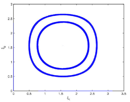
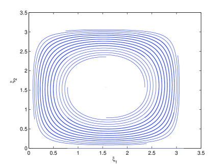
Figure 1: Phase portraits of the slow system (3.3)-(3.4) with $V=0$, $a=0.7$ and $\sigma=0$ (no noise): $\varepsilon=0$ (top); $\varepsilon=0.05$ (bottom).

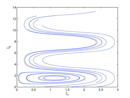
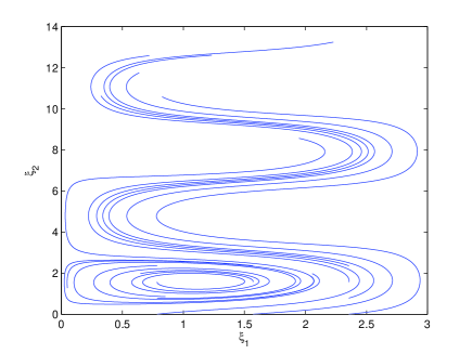
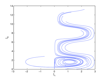
Figure 2: Sample particle orbits of the slow system (3.3) and (3.4) with $V=0.3$ and $a=0.7$: $\varepsilon=0$ and $\sigma=0$ (top, no noise); $\varepsilon=0.05$ and $\sigma=0$ (middle, no noise); $\varepsilon=0.05$ and $\sigma=0.01$ (bottom, with noise).

(

(

(

Figure 3: First exit time for the slow system (3.3) and (3.4) with $\varepsilon=0.05$, $a=0.7$ and $\sigma=0.01$: (a) $V=0$, (b) $V=0.1$, (c) $V=0.5$ and (d) $V=0.65$.

a) b)
c) d)

(

(

(

(

Figure 4: Escape probability for the slow system (3.3) and (3.4) with $V=0$, $\varepsilon=0.05$, $a=0.7$ and $\sigma=0.01$: (a) escape through $\xi_{2}=\pi$ (settling direction or physical bottom boundary), (b) escape through $\xi_{2}=0$ (physical top boundary), (c) escape through $\xi_{1}=0$ (left boundary), and (d) escape through $\xi_{1}=\pi$ (right boundary).

a) b)
c) d)

(

(

(

(

Figure 5: Escape probability for the slow system (3.3) and (3.4) with $V=0.1$, $\varepsilon=0.05$, $a=0.7$ and $\sigma=0.01$: (a) Escape through $\xi_{2}=\pi$ (settling direction or physical bottom boundary), (b) escape through $\xi_{2}=0$ (physical top boundary), (c) escape through $\xi_{1}=0$ (left boundary), and (d) escape through $\xi_{1}=\pi$ (right boundary).

a) b)
c) d)

(

(

(

(

Figure 6: Escape probability for the slow system (3.3) and (3.4) with $V=0.1$, $\varepsilon=0.05$, $a=0.7$ and $\sigma=0.01$: (a1) and (a2) are Figure 5(a) splitting at the deterministic heteroclinic orbit $a\sin\xi_{1}\sin\xi_{2}-V\xi_{1}=0$; (c1) and (c2) are Figure 5(c) splitting at the same heteroclinic orbit.

a1) a2)
c1) c2)

(

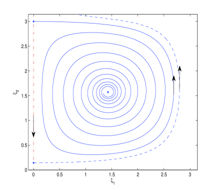
Figure 7: Deterministic stable manifold $W^{s}(0,\pi-\sin^{-1}(\frac{V}{a}))$ (Blue solid curve) and unstable manifold $W^{u}(0,\sin^{-1}(\frac{V}{a}))$ (Blue dashed curve) for the slow system (3.3) and (3.4): $V=0.1$, $\varepsilon=0.05$, $a=0.7$, and $\sigma=0$ (no noise). Two equilibrium points are $(0,\pi-\sin^{-1}(\frac{V}{a}))$ and $(0,\sin^{-1}(\frac{V}{a}))$.

Figure 8: Escape probability (Light blue color) for particles through the left boundary for the slow system (3.3) and (3.4) with $V=0.1$, $\varepsilon=0.05$, $a=0.7$ and $\sigma=0.01$ (with noise), together with deterministic stable manifold $W^{s}(0,\pi-\sin^{-1}(\frac{V}{a}))$ and unstable manifold $W^{u}(0,\sin^{-1}(\frac{V}{a}))$ (Red curves).

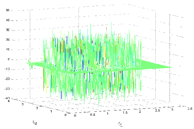
Figure 9: Difference between the particle settling times for the deterministic case ($\sigma=0$) and the random case ($\sigma=0.01$) of the slow system (3.3) and (3.4): $V=0.1$, $\varepsilon=0.05$ and $a=0.7$.

3.2 Deterministic Case

We recall the results, by one of the present authors, of the deterministic motion of aerosol particles in a cellular flow [11].

When the settling velocity in still fluid is zero, i.e., $V=0$ (and also $\sigma=0$), particles are trapped in the cell either in circular motion (with no inertial, $\varepsilon=0$) or spiralling motion (with inertial, $\varepsilon>0$), as shown in Figure 1 (top) and (bottom), respectively.

When the settling velocity in still fluid is non-zero, i.e., $V>0$, in the case with inertial absent ($\varepsilon=0$) and noise absent ($\sigma=0$), the particles in the area surrounded by the heteroclinic orbit $a\sin\xi_{1}\sin\xi_{2}-V\xi_{1}=0$ connecting the equilibrium points $(0,\sin^{-1}(V/a))$ and $(0,\pi-\sin^{-1}(V/a))$, are trapped inside it, with the equilibrium point $(\cos^{-1}(V/a),\pi/2)$ as a center. But the particles in the remaining area settle to the bottom of the fluid. With an arbitrarily small inertial effect ($0<\varepsilon\ll 1$ and also $\sigma=0$), the heteroclinic orbit breaks and it leads to the settling of almost all particles, with the equilibrium point $(\cos^{-1}(V/a)),\pi/2)$ becoming an unstable spiral. Figure 7 is the stable manifold $W^{s}(0,\pi-\sin^{-1}(V/a))$ (Blue solid curve) and unstable manifold $W^{u}(0,\sin^{-1}(V/a))$ (Blue dashed curve) when inertial presents ($\varepsilon=0.05$ and also $\sigma=0$).

3.3 Stochastic Case

For zero settling velocity in still fluid ($V=0$), we note that all particles are trapped in a fluid cell $D=(0,\pi)\times(0,\pi)$ when noise is absent. Figure 1 shows the particle orbits in this case.

For non-zero settling velocity in still fluid ($V\neq 0$), when noise is absent ($\sigma=0$ ), all particles settle to the fluid bottom; see Figure 2 (top, middle). But when noise is present ($\sigma\neq 0$), some particles exit the cell not only by settling. Figure 2 (bottom) shows that, with small noise ($\sigma=0.01$), some particles indeed exit the cell from the vertical side boundary $\xi_{1}=0$.

In fact, when noise is present, all particles will exit, no matter the settling velocity in still fluid $V$ is zero or non-zero. Figure 3 indicates that with noise, particles will all exit from a fluid cell in finite time, almost surely. In the following we only consider the case with noise.

Figures 4 — 5 plot the escape probability through four side boundaries, for zero or non-zero $V$ (settling velocity in still fluid) values. When a particle reaches or is on a side boundary, it is regarded as ‘having escaped through’ that part of the boundary. In other words, particles on a side boundary have escape probability $1$ (you see this in these figures). When $V=0$, the particles escape the cell through each of the four side boundaries with similar or equal likelihood (Figure 4), as there is no preferred direction for particles due to zero settling velocity $V=0$ (in still fluid). With non-zero $V$, particles almost surely do not escape through the right side boundary $\xi_{1}=\pi$. In fact, the inertial particles either settle to the physical bottom or exit from the left side boundary $\xi_{1}=0$. Figure 5 displays the escape probability for $V=0.1$, through each of the four side boundaries of the fluid cell. Although most particles settle (Figure 5 (a)), some particles escape the fluid cell through the left side boundary (Figure 5 (c)). See Figure 6 for a split view of this phenomenon.

To examine this phenomenon more carefully, we draw the stable manifold $W^{s}(0,\pi-\sin^{-1}(V/a))$ and unstable manifold $W^{u}(0,\sin^{-1}(V/a))$ for the deterministic system ($\sigma=0$) in Figure 7. As shown in Figure 8, inertial particles with significant likelihood of escaping through the left side boundary are near or on the stable manifold $W^{s}(0,\pi-\sin^{-1}(V/a))$. In other words, some (but not all) inertial particles near or on this stable manifold are resistent to settling in the stochastic case. This resistance is quantified by the escape probability for a particle to get out of the fluid cell through the left side boundary. More specifically, the difference between the inertial particle settling times for deterministic case ($\sigma=0$) and a random case ($\sigma=0.01$) is shown in Figure 9. We observe that the inertial particles near or on the stable manifold $W^{s}(0,\pi-\sin^{-1}(V/a))$ could have either a longer or shorter settling time, compared with the deterministic case. This indicates that the noise could either delay or enhance the settling (although we do not know the reason), and the stable manifold is an agent facilitating this behavior. However, the overall impact of noise appears to delay the settling, as the averaged difference over the cell $(0,\pi)\times(0,\pi)$ is $-0.0133$ for noise intensity $\sigma=0.01$, while this averaged value is $-0.1168$ for a stronger noise with $\sigma=0.1$.

3.4 Conclusions

Let the settling velocity in still fluid be non-zero (i.e., $V\neq 0$).
(i) In the classical case (no inertial: $\varepsilon=0$ and no noise: $\sigma=0$), the particles surrounded inside a heteroclinic orbit are trapped inside it and all the other particles settle to the bottom of this cellular fluid flow.
(ii) In the case with only small inertia influence ($0<\varepsilon\ll 1,\sigma=0$), the heteroclinic orbit breaks up to form a stable manifold $W^{s}$ and an unstable manifold $W^{u}$, the trapped particles then settle, i.e., all inertial particles settle.
(iii) However, when the noise is present ($0<\varepsilon\ll 1,\sigma\neq 0$), although most inertial particles still settle, some particles near or on the deterministic stable manifold $W^{s}$ escape the fluid cell through the left side boundary, with non-negligible likelihood. Thus, inertial particle motions occur in two adjacent fluid cells in random cases, but confine in single cells in the deterministic case.

In fact, noise could either delay settling for some particles or enhance settling for others, and the deterministic stable manifold is an agent to facilitate this phenomenon. Overall, noise appears to delay the settling in an averaged sense.

References

- [1] L. Arnold, Random Dynamical Systems. Springer-Verlag, New York, 1998.
- [2] K. J. Beven, P. C. Chatwin and J. H. Millbank, Mixing and Transport in the Environment, John Wiley & Sons, New York, 1994.
- [3] N. Berglund and B. Gentz, Noise-Induced Phenomena in Slow-Fast Dynamical Systems, Springer-Verlag, 2006.
- [4] M. M. Clark, Transport Modeling for Environmental Engineers and Scientists, John Wiley and Sons, New York, 1996.
- [5] J. Duan, K. Lu and B. Schmalfuss, Smooth stable and unstable manifolds for stochastic evolutionary equations, J. Dynam, Differential Equations, 16 (2004), 949-972.
- [6] M. I. Freidlin and A. D. Wentzell, Random Perturbations of Dynamical Systems, Springer-Verlag, 2nd Edition, 1998, Chapter 7.
- [7] H. Fu, X. Liu and J. Duan, Slow manifolds for multi-time-scale stochastic evolutionary systems. Comm. Math. Sci., 2013, Vol. 11, No. 1, pp. 141-162.
- [8] G. Haller and T. Sapsis, Where do inertial particles go in fluid flows? Phys. D 237 (2008), 573-583.
- [9] C. K. R. T. Jones, Geometric singular perturbation theory, Lecture Notes in Math, 1609 (1995), 44-118.
- [10] Y. Kabanov and S. Pergamenshchikov, Two-scale stochastic systems: asymptotic analysis and control. Springer-Verlag, New York, 2003.
- [11] J. Rubin, C. K. R. T. Jones and M. Maxey, Settling and Asymptotics of Aerosol Particles in a Cellular Flow Field, J. Nonlinear Sci. 5 (1995), 337-358.
- [12] B. Schmalfuss and K. R. Schneider, Invriant manifolds for random dynamical systems with slow and fast variables. J. Dyn. Diff. Eqns. 20 (2008), 133-164.
- [13] J. L. Schnoor, Environmental Modeling: Fate and Transport of Pollutants in Water, Air and Soil, John Wiley and Sons, New York, 1996.
- [14] X. Sun, J. Duan and X. Li, An impact of noise on invariant manifolds in nonlinear dynamical systems. J. Math. Phys., 51 (2010), 042702.
- [15] W. Wang, A. J. Roberts and J. Duan, Large deviations and approximations for slow fast stochastic reaction diffusion equations. J. Differential Equations 253 (2012), no. 12, 3501-3522.
- [16] C. Xu and A. J. Roberts, On the low-dimensional modelling of Stratonovich stochastic differential equations. Physica A, 225:62–80, 1996.