Hidden-Symmetry-Protected Topological Semimetals on a Square Lattice

Abstract

We study a two-dimensional fermionic square lattice, which supports the existence of two-dimensional Weyl semimetal, quantum anomalous Hall effect, and $2\pi$-flux topological semimetal in different parameter ranges. We show that the band degenerate points of the two-dimensional Weyl semimetal and $2\pi$-flux topological semimetal are protected by two distinct novel hidden symmetries, which both corresponds to antiunitary composite operations. When these hidden symmetries are broken, a gap opens between the conduction and valence bands, turning the system into a insulator. With appropriate parameters, a quantum anomalous Hall effect emerges. The degenerate point at the boundary between the quantum anomalous Hall insulator and trivial band insulator is also protected by the hidden symmetry.

Introduction.—The research on topological phases is becoming an increasingly important theme in condensed matter physics. Topological matters are classified according to topological invariants rather than symmetriesHasan ; Qi . Depending on the dimensionality and the symmetry classes specified by time reversal symmetry and particle-hole symmetry, gapped systems can be classified into ten types of topological phasesSchnyder , such as the integer quantum Hall statesThouless , quantum anomalous Hall insulatorHaldane ; LiuQA , topological insulatorsKane , chiral topological superfluidsRead , and helical topological superfluids or superconductorsQi2 . More recently, physicists have found that, besides the gapped systems, gapless systems can also support topological phases, i.e., topological semimetalsWan ; Xu ; Burkov1 ; Burkov2 ; Fang ; Zyuzin ; Sun ; Jiang ; Hosur ; Delplace .

Topological semimetals have band structures with band-touching points in momentum space, where the isolated band degeneracy occurs. In general, at these kind of band-degeneracy points, there exist singularities of a Berry field. Around the singularities, vortex structures in two-dimensions or monopoles in three dimensions appear. These vortices or monopoles with opposite topological charges are separated from each other in momentum space due to symmetries and thus cannot be destroyed by the mutual annihilation of pairs with opposite topological charges. In three dimensions, the band degeneracy at isolated points can be accidental Wan ; Herring . The robustness of the accidental degeneracy depends on its codimensionBurkov1 . However, such accidental band degeneracies are vanishingly improbable in one and two dimensions if there are not additional symmetry constraintsBalents . Therefore, in two dimensions, the band degeneracy at isolated points must be protected by symmetries.

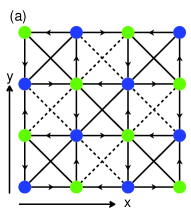
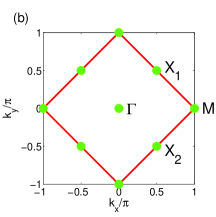
Figure 1: (Color online). (a) Schematic of the lattices. The arrows represent the accompanying phase of hopping $\gamma$ and the dashed lines indicate a $\pi$ accompanying phase; the blue and green filled circles represent the lattice sites of sublattices $A$ and $B$, respectively. (b) The first Brillouin zone, which is surrounded by red lines. Here, the green filled circles represent symmetry points denoted by $\Gamma$, $M$ and $X_{1,2}$, respectively.

Discrete symmetries with antiunitary operators play a crucial role in topological phases, for instance, time-reversal symmetry and particle-hole symmetry offer a base for classifying the topological phases into ten classesSchnyder . In condensed matter physics, besides time-reversal and particle-hole symmetries, there exists a class of hidden symmetries, which are seldom studied in the literature. These hidden symmetries are discrete symmetries with antiunitary composite operators, which, in general, consist of translation, complex conjugation and sublattice exchange, and sometimes also include local gauge transformation and rotation. Although a lot of researches were done focusing on Dirac or Weyl semimetals in two-dimensional lattices in recent yearsLim ; Hou ; Goldman ; Bercioux ; Goldman2 , few of them have involved the relation between the band degeneracies and the above hidden symmetries. In this Letter, we will study this relation and take a square lattice as an example. This square lattice supports the existence of topological semimetals and a quantum anomalous Hall effect in different parameter ranges. The topological semimetals appearing in this model include a two-dimensional Weyl semimetal and a $2\pi$-flux topological semimetal, which are protected by different hidden symmetries. Moreover, we show that the Weyl node at the phase boundary between quantum anomalous Hall insulator and trivial band insulator is protected by the hidden symmetry as well. In order to show the ubiquity of hidden-symmetry-protected topological semimetals, we also present other two-dimensional lattices with different hidden symmetries in the Supplemental MaterialSM .

Model.—We consider a square lattice as shown in Fig.1. Because of the presence of the accompanying phases of hopping, the translation symmetry is broken, then the lattice is divided into two sublattices denoted $A$ and $B$. This square lattice has a lattice spacing $d$ and, for simplicity, we assume $d=1$ in the following process. For each sublattice, the primitive lattice vectors are defined as ${\bm{a}}_{1}=(1,1)$ and ${\bm{a}}_{2}=(1,-1)$. For the reciprocal lattice, the corresponding primitive reciprocal lattice vectors are ${\bm{b}}_{1}=(\pi,\pi)$ and ${\bm{b}}_{2}=(\pi,-\pi)$.

The corresponding total Hamiltonian consists of three parts such as the square lattice Hamiltonian $H_{0}$, the diagonal Hamiltonian $H_{1}$ and the staggered potential Hamiltonian $H_{2}$, i.e., $H=H_{0}+H_{1}+H_{2}$, which can be written as,

$$H_{0} = -t\sum_{i\in A}[e^{-i\gamma}a^{\dagger}_{i}b_{i+\hat{x}}+e^{-i\gamma}a^{\dagger}_{i}b_{i-\hat{x}}+e^{i\gamma}a^{\dagger}_{i}b_{i+\hat{y}}$$ (1)

$$+e^{i\gamma}a^{\dagger}_{i}b_{i-\hat{y}}]+{\rm H.c.},$$

and

$$H_{1} = -t_{1}\sum_{i\in A}[a^{\dagger}_{i}a_{i+\hat{x}+\hat{y}}-a^{\dagger}_{i}a_{i+\hat{x}-\hat{y}}]$$ (2)

$$+t_{1}\sum_{i\in B}[b^{\dagger}_{i}b_{i+\hat{x}+\hat{y}}-b^{\dagger}_{i}b_{i+\hat{x}-\hat{y}}]+{\rm H.c.},$$

and

$$H_{2}=v\sum_{i\in A}a^{\dagger}_{i}a_{i}-v\sum_{j\in B}b^{\dagger}_{j}b_{j},$$ (3)

where $a_{i}$ destructs a particle at the site $i$ in sublattice $A$ and $b_{j}$ destructs a particle at the site $j$ in sublattice $B$; $\hat{x}\equiv(1,0)$ and $\hat{y}\equiv(0,1)$ represent the unit vectors in the $x$ and $y$ directions, respectively; $0<\gamma<\pi/2$ is a phase factor along with hopping; $t$ is the hopping amplitude along the $x$ and $y$ directions and $t_{1}$ the hopping amplitude along the diagonal directions; $v$ is the magnitude of staggered potential. In the following process, we will consider the model in three parameter ranges such as (i) $0<\gamma<\pi/2$, $t\neq 0$, $t_{1}=0$, $v=0$, i.e. $H=H_{0}$, (ii) $0<\gamma<\pi/2$, $t\neq 0$, and at least one of $t_{1}$ and $v$ being nonzero, and (iii) $\gamma=0$, $t\neq 0$, $t_{1}\neq 0$, $v=0$, which support the existence of a two-dimensional Weyl semimetal, quantum anomalous Hall effect, and $2\pi$-flux topological semimetal, respectively.

Two-dimensional Weyl semimetals.—First, we consider the first parameter range with $0<\gamma<\pi/2$, $t\neq 0$, $t_{1}=0$ and $v=0$, i.e. $H=H_{0}$. We take Fourier transformation to annihilation operators as ${a}_{{\bm{k}}}=\frac{1}{\sqrt{N}}\sum_{i}{a}_{i}e^{-i{\bm{k}}\cdot{\bm{R}}^{A}_{i}}$, ${b}_{{\bm{k}}}=\frac{1}{\sqrt{N}}\sum_{i}{b}_{i}e^{-i{\bm{k}}\cdot{\bm{R}}^{B}_{i}}$Bena and define the two-component annihilation operator as ${\eta}_{{\bm{k}}}\equiv\frac{1}{\sqrt{2}}[{a}_{{\bm{k}}},{b}_{{\bm{k}}}]^{T}$. The Hamiltonian (1) can be rewritten as $H=\sum_{{\bm{k}}}{\eta}_{{\bm{k}}}^{\dagger}{\cal H}({\bm{k}}){\eta}_{{\bm{k}}}$ with

$${\cal H}({\bm{k}}) = -\cos\gamma\Omega_{+}\sigma_{x}-\sin\gamma\Omega_{-}\sigma_{y},$$ (4)

where $\Omega_{+}=2t(\cos k_{x}+\cos k_{y})$ and $\Omega_{-}=2t(\cos k_{x}-\cos k_{y})$; $\sigma_{x}$ and $\sigma_{y}$ are the Pauli matrices. Diagonalizing Eq.(4), we obtain the dispersion relation as $E({{\bm{k}}})=\pm\sqrt{\cos^{2}\gamma\Omega_{+}^{2}+\sin^{2}\gamma\Omega_{-}^{2}}$.

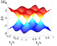
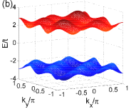
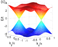
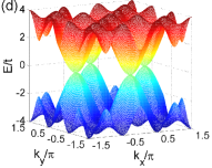
Figure 2: (Color online). The energy dispersions for (a)a two-dimensional Weyl semimetal with $\gamma=\pi/4$, $t_{1}=0$, $v=0$; (b)a quantum anomalous Hall insulator with $\gamma=\pi/4$, $t_{1}=0.8t$, $v=0.2t$; (c) the boundary between the quantum anomalous Hall insulator and trivial band insulator with $\gamma=\pi/4$, $t_{1}=0.5t$, $v=2t$; (d)a $2\pi$-flux topological semimetal with $\gamma=0$, $t_{1}=t$ and $v=0$.

Figure 2(a) shows the dispersion relation for $\gamma=\pi/4$. From the dispersion relation, we find that the conduction and valence bands are touched at symmetry points $X_{1,2}=(\pi/2,\pm\pi/2)$ in the Brillouin zone as denoted in Fig.1(b). Near these degenerate points, the band structure has a conelike shape and is linear. Thus, the quasiparticles and quasiholes behave like massless relativistic fermions. Around these degenerate points, the single-particle Hamiltonian (4) can be linearized as

$${h}({\bm{p}}) = 2t\cos\gamma(p_{x}\pm p_{y})\sigma_{x}+2t\sin\gamma(p_{x}\mp p_{y})\sigma_{y},$$ (5)

where ${\bm{p}}={\bm{k}}-X_{i}$ with $i=1,2$; the two signs indicate the linearized Hamiltonian around the two distinct touched points $X_{1}$ and $X_{2}$, respectively. The Hamiltonian (5) has the form like $h({\bm{p}})=\sum_{ij}v_{ij}p_{i}\sigma_{j}$, based on which, though the $\gamma_{5}$ matrix is absent in $(2+1)$-dimensions, we can define the chirality for two-dimensional massless relativistic fermions as $w=\textrm{sgn}[\det(v_{ij})]=\pm 1$. We can regard the chiral relativistic fermions as two-dimensional Weyl fermions. From Eq.(5) and the definition of the chirality, we have $w=-1,+1$ for Weyl nodes located at the degenerate points $X_{1}$ and $X_{2}$, respectively. It turns out that $X_{1}$ and $X_{2}$ have opposite chirality.

The Weyl nodes can also be interpreted as topological defects, i.e. vortices, of the planar vector field in momentum space like ${\bm{h}}=(h_{x},h_{y})$ with $h_{x}=-2t\cos\gamma(\cos k_{x}+\cos k_{y})$ and $h_{y}=-2t\sin\gamma(\cos k_{x}-\cos k_{y})$, which is defined by using the coefficients of Pauli matrices in Eq.(4). The corresponding topological invariant is the winding number defined as Sun

$$w=\oint_{\cal C}\frac{d{{\bm{k}}}}{2\pi}\cdot\left(\hat{h}_{x}\nabla\hat{h}_{y}-\hat{h}_{y}\nabla\hat{h}_{x}\right),$$ (6)

where $\hat{h}_{i}={h_{i}}/{|{{\bm{h}}}|}$. For the definition Eq.(6), we calculate that the winding number of the vortices at the degenerate points is $+1$ or $-1$, which is consistent with the chirality defined above.

Symmetry protection.—The model in the first parameter range, i.e., $0<\gamma<\pi/2$, $t\neq 0$, $t_{1}=0$ and $v=0$, has a hidden symmetry, which is a discrete symmetry with an antiunitary compositor operator. We will show that this hidden symmetry supports the existence of isolated band degeneracy. The corresponding composite symmetry operator can be written as,

$$\Upsilon=\sigma_{x}KT_{\hat{x}},$$ (7)

where $T_{\hat{x}}$ is a translation operator which moves the lattice by $\hat{x}$ along the $x$ direction; $K$ is the complex conjugation operator, which can also be regarded as a time-reversal operator for spinless particles; $\sigma_{x}$ is the Pauli matrix representing the sublattice exchange. The model considered here is invariant under this composite transformation, i.e., $H=\Upsilon H\Upsilon^{-1}$, where the inverse operator is $\Upsilon^{-1}=\sigma_{x}KT_{\hat{x}}^{-1}$. The $\Upsilon$ operator has the character as $\Upsilon^{2}=T_{2\hat{x}}$.

The Bloch function has the form $\Psi_{{\bm{k}}}({\bm{r}})=[u^{(1)}({\bm{r}}),u^{(2)}({\bm{r}})]^{T}e^{i{\bm{k}}\cdot{\bm{r}}}$. The symmetry operator $\Upsilon$ acts on the Bloch function as follows

$$\Upsilon\Psi_{{\bm{k}}}({\bm{r}}) = \left(\matrix{u^{(2)*}_{{\bm{k}}}({\bm{r}}-\hat{x})e^{ik_{x}}\cr u^{(1)*}_{{\bm{k}}}({\bm{r}}-\hat{x})e^{ik_{x}}}\right)e^{-i{\bm{k}}\cdot{\bm{r}}}=\Psi^{\prime}_{{\bm{k}}^{\prime}}({\bm{r}}).$$ (8)

Because $\Upsilon$ is the symmetry operator of the system, $\Psi^{\prime}_{{\bm{k}}^{\prime}}({\bm{r}})$ must be a Bloch wave function of the system. Thus, we obtain ${\bm{k}}^{\prime}=-{\bm{k}}$, $u^{(1)}_{{\bm{k}}^{\prime}}({\bm{r}})=u^{(2)*}_{{\bm{k}}}({\bm{r}}-\hat{x})e^{ik_{x}}$ and $u^{(2)}_{{\bm{k}}^{\prime}}({\bm{r}})=u^{(1)*}_{{\bm{k}}}({\bm{r}}-\hat{x})e^{ik_{x}}$. From Eq.(8), it is easy to show that the operator $\Upsilon$ has the effect when acting on wave vectors as $\Upsilon:{\bm{k}}\rightarrow-{\bm{k}}={\bm{k}}^{\prime}$. If ${\bm{k}}^{\prime}={\bm{k}}+{\bm{K}}_{m}$, where ${\bm{K}}_{m}$ is the reciprocal lattice vector, then we can say that ${\bm{k}}$ is a $\Upsilon$-invariant point in momentum space. In the Brillouin zone, the $\Upsilon$-invariant points are the points $\Gamma,M$ and $X_{1,2}$, which are marked by green balls in Fig.1(b). Suppose that ${\bm{G}}$ represents a $\Upsilon$-invariant point, then we have $\Upsilon\Psi_{{\bm{G}}}({\bm{r}})=\Psi^{\prime}_{{\bm{G}}}({\bm{r}})$. Because of the equation $\Upsilon H\Upsilon^{-1}=H$, $\Psi_{{\bm{G}}}({\bm{r}})$ and $\Psi^{\prime}_{{\bm{G}}}({\bm{r}})$ are both the eigenstates of Hamiltonian $H$ and have the same eigenenergy $E({\bm{G}})$. After the symmetry operator acts on the Bloch function two times, we have $\Upsilon^{2}\Psi_{{\bm{G}}}({\bm{r}})=T_{2\hat{x}}\Psi_{{\bm{G}}}({\bm{r}})=e^{-2iG_{x}}\Psi_{{\bm{G}}}({\bm{r}})$, where $G_{x}$ is the $x$ component of ${\bm{G}}$. From the above equation, we obtain $\Upsilon^{2}=e^{-2iG_{x}}$, which is a function of the wave vector. Substituting the wave vectors of the $\Upsilon$-invariant points $\Gamma,M$ and $X_{1,2}$, we obtain $\Upsilon^{2}=1$ at $\Gamma,M$ and $\Upsilon^{2}=-1$ at $X_{1,2}$. If a system is invariant under the action of an antiunitary operator and the square of the operator is not equal to 1, there must be degeneracy protected by this antiunitary operatorSM . Thus, the bands must be degenerate at the points $X_{1,2}$ in the Brillouin zone, which is consistent with the Weyl nodes obtained from dispersion relation.

Quantum anomalous Hall effect.— For the second parameter range, i.e., $0<\gamma<\pi/2$, $t\neq 0$, and at least one of $t_{1}$ and $v$ being nonzero, there are nonvanishing $H_{1}$ or $H_{2}$ in the total Hamiltonian. It is easy to show that $H_{1}$ and $H_{2}$ violate the hidden symmetry, i.e. $\Upsilon H_{1,2}\Upsilon^{-1}\neq H_{1,2}$. Thus, both of them can remove the degeneracy at Weyl nodes and open a gap between the valence and conduction bands, turning the system into a insulator.

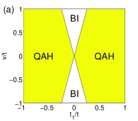
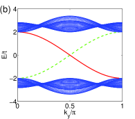
Figure 3: (Color online). (a) Phase diagram for insulators. Here, QAH and BI represent quantum anomalous Hall insulator and trivial band insulator, respectively. (b) The edge states of the quantum anomalous Hall phase for $\gamma=\pi/4$, $t_{1}=0.8t$ and $v=0.2t$. Red solid line and green dashed line represent edge states at two opposite edges, respectively.

The corresponding Bloch Hamiltonian can be written as

$${\cal H}({\bm{k}}) = -\cos\gamma\Omega_{+}\sigma_{x}-\sin\gamma\Omega_{-}\sigma_{y}+m\sigma_{z},$$ (9)

where $m=v-2t_{1}[\cos(k_{x}+k_{y})-\cos(k_{x}-k_{y})]$. Comparing with the first parameter range, there is an additive mass term. Diagonalizing the above equation, we obtain $E({{\bm{k}}})=\pm\sqrt{\cos^{2}\gamma\Omega_{+}^{2}+\sin^{2}\gamma\Omega_{-}^{2}+m^{2}}$. Figure 2(b) shows that a gap between the conduction and valence bands is opened by the mass term.

For an insulator, we can always characterize the occupied bands with the first Chern number calculated based on Berry phases in the first Brillouin zone. The corresponding first Chern number can be defined as $C_{1}=\frac{1}{4\pi}\int_{BZ}dk_{x}dk_{y}\hat{{\bm{h}}}\cdot\left({\partial\hat{{\bm{h}}}}/{\partial k_{x}}\times{\partial\hat{{\bm{h}}}}/{\partial k_{y}}\right)$, where $\hat{{\bm{h}}}={\bm{h}}/|{\bm{h}}|$ with ${\bm{h}}$ being the coefficients of the Pauli matrices in Eq.(9). For quantum anomalous Hall states, the first Chern number must not be zero. This is just the case when the mass term at the two distinct degenerate points has opposite sign, and the system has a nontrivial first Chern number $C_{1}=\pm 1$Haldane . The vanishing mass at one of the two distinct degenerate points $X_{1}$ and $X_{2}$, i.e., $v=\pm 4t_{1}$, defines the boundary between quantum anomalous Hall insulator and trivial band insulator in the phase diagram as shown in Fig.3(a). In the regime of the quantum anomalous Hall insulator, chiral edge states at each edge appear, which are shown in Fig.3(b).

At the boundary between the quantum anomalous Hall insulator and trivial band insulator, i.e., $v=\pm 4t_{1}$, one of the two distinct Weyl nodes in the Brillouin zone reappears, as shown in Fig.2(c). This can be explained by the recovery of the hidden symmetry $\Upsilon$ at some points in momentum space. For instance, when $v=-4t_{1}$ is satisfied, the mass term in Eq.(9) vanishes at $X_{1}$, while it still exists at $X_{2}$. Thus, the symmetry $\Upsilon$ is recovered at $X_{1}$ point, i.e. $\Upsilon{\cal H}(X_{1})\Upsilon^{-1}={\cal H}(X_{1})$. Then, the Weyl node reappears at $X_{1}$ but does not at $X_{2}$. Similarly, for $v=4t_{1}$, the symmetry is recovered at $X_{2}$, but not at $X_{1}$, i.e., $\Upsilon{\cal H}(X_{2})\Upsilon^{-1}={\cal H}(X_{2})$ , then the Weyl node reoccurs at $X_{2}$ but not at $X_{1}$.

$2\pi$-flux topological semimetals.— Now, we consider the third parameter range, i.e., $\gamma=0$ and $v=0$ for the total Hamiltonian $H$. For this special case, the Bloch Hamiltonian can be written as,

$${\cal H}({\bm{k}}) = -\Omega_{+}\sigma_{x}-\Omega_{z}\sigma_{z},$$ (10)

where $\Omega_{z}=2t_{1}[\cos(k_{x}+k_{y})-\cos(k_{x}-k_{y})]$. Diagonalizing the Hamiltonian, we obtain the dispersion relation as $E({\bm{k}})=\pm\sqrt{\Omega_{+}^{2}+\Omega_{z}^{2}}$. The conduction and valence bands are touched at point $M$ in the Brillouin zone as shown in Fig.2(d). Around the degenerate point, the bands have a quadratic dispersion relation. For instance, retaining only the lowest terms around the degenerate point $M$, i.e., $(\pi,0)$, the Bloch Hamiltonian (10) can be written as,

$${\cal H}({\bm{k}}) = -t(p_{x}^{2}-p_{y}^{2})\sigma_{x}-4t_{1}p_{x}p_{y}\sigma_{z},$$ (11)

where ${\bm{p}}={\bm{k}}-M$. For each band crossing, from the formula (6), we can calculate a winding number with value of $+2$ or $-2$. These band crossings correspond to vortices with $2\pi$ or $-2\pi$ Berry flux and can also be regarded as a double-Weyl node consisting of two Weyl nodes with the same chirality, which is similar to the topological semimetal protected by $D_{4}$ point-group symmetrySun .

The $2\pi$-flux nodes in this parameter range can be interpreted by the protection of symmetry. In this parameter range, the model has a new composite symmetry such that $\Upsilon^{\prime}H{\Upsilon^{\prime}}^{-1}=H$ with

$$\Upsilon^{\prime}=\sigma_{x}KC_{4}T_{\hat{x}},$$ (12)

where $C_{4}$ is a rotation operation by $\pi/2$ around the normal vector of the $x-y$ plane. This composite antiunitary operator $\Upsilon^{\prime}$ has a more $C_{4}$ rotation than the operator $\Upsilon$ and has the property that ${\Upsilon^{\prime}}^{2}=C_{2}T_{{\bm{a}}_{1}}$ with $C_{2}=C_{4}^{2}$. The action of symmetry operator $\Upsilon^{\prime}$ on wave vectors has the effect that $\Upsilon^{\prime}:(k_{x},k_{y})\rightarrow(-k_{y},k_{x})$. Thus, under this symmetry operation, the Bloch Hamiltonian is transformed as $\Upsilon^{\prime}{\cal H}(k_{x},k_{y}){\Upsilon^{\prime}}^{-1}={\cal H}(-k_{y},k_{x})$. It is very easy to show that the Bloch Hamiltonian is invariant at the point $M=(\pi,0)$ and point $\Gamma=(0,0)$ in the Brillouin zone. It is easy to show that $\Upsilon^{\prime 2}=C_{2}T_{{\bm{a}}_{1}}=-1$ at point $M$, while it is equal to $1$ at point $\Gamma$. Therefore, the bands must be degenerate at point $M$ in the Brillouin zone, which is consistent with the dispersion relation calculated above.

The symmetry $\Upsilon^{\prime}$ also guarantees that the dispersion relation is quadratic instead of linear near the degenerate point. The corresponding Bloch Hamiltonian can be written in the form ${\cal H}(k_{x},k_{y})=f(k_{x},k_{y})\sigma_{x}+g(k_{x},k_{y})\sigma_{z}$, where $f(k_{x},k_{y})$ and $g(k_{x},k_{y})$ are functions of $k_{x}$ and $k_{y}$. On one hand, we have ${\cal H}(-k_{y},k_{x})=f(-k_{y},k_{x})\sigma_{x}+g(-k_{y},k_{x})\sigma_{z}$, on the other hand, $\Upsilon^{\prime}{\cal H}(k_{x},k_{y}){\Upsilon^{\prime}}^{-1}=f(k_{x},k_{y})\sigma_{x}-g(k_{x},k_{y})\sigma_{z}$. Therefore, due to $\Upsilon^{\prime}{\cal H}(k_{x},k_{y}){\Upsilon^{\prime}}^{-1}={\cal H}(-k_{y},k_{x})$, we obtain the equations $f(k_{x},k_{y})=f(-k_{y},k_{x})$ and $g(k_{x},k_{y})=-g(-k_{y},k_{x})$. Since the degenerate point is located at $M$ in the Brillouin zone, the functions $f(k_{x},k_{y})$ and $g(k_{x},k_{y})$ can be expanded at point $M$ in Taylor series as $f(k_{x},k_{y})=f({M})+\sum_{i}c_{i}p_{i}+\frac{1}{2}\sum_{ij}c_{ij}p_{i}p_{j}+\cdots$ and $g(k_{x},k_{y})=g({M})+\sum_{i}d_{i}p_{i}+\frac{1}{2}\sum_{ij}d_{ij}p_{i}p_{j}+\cdots$. Considering the above equations satisfied by $f(k_{x},k_{y})$ and $g(k_{x},k_{y})$, it is easy to show that all the first order terms vanish for $f(k_{x},k_{y})$ and $g(k_{x},k_{y})$, and the lowest order nonvanishing terms are the second order terms, which is consistent with Eq.(11). Therefore, the fact that the dispersion relation is quadratic near the degenerate point can be interpreted from the protection of symmetry. More general and detailed proof is presented in Supplemental MaterialSM .

Experimental techniques for physical realization–The high controllability and large number of detection techniques of cold atoms in optical lattices make them a platform we can use to realize many models in condensed matter physics. The model considered by us can be realized by applying ${}^{40}{\rm K}$ cold atoms trapped in spin-dependent optical latticeBloch . The accompanying phase of hopping can be realized by laser-induced gauge potentialsHou ; Lin ; Aidelsburger . The interferometric approach proposed by Abanian et al.Abanin can be used to detect the winding number at degenerate points of topological semimetals and the Chern number of the quantum anomalous Hall insulator. The Chern number of insulators can also be measured with the time-of-flight method proposed by Alba et al.Alba and the method of measuring Bloch eigenstates at symmetric points of the Brillouin zone proposed by Liu et al.Liuxj .

Conclusion.—In summary, we have shown that, besides time-reversal symmetry and particle-hole symmetry, there exists a class of discrete symmetries with antiunitary composite operators contributing to the protection of degeneracies in two-dimensional systems. In order to clearly manifest the close relation between this kind of hidden symmetries and degeneracies in two-dimensional systems, we have studied a fermionic square lattice for example. This model supports the existence of a two-dimensional Weyl semimetal, quantum anomalous Hall effect, and $2\pi$-flux topological semimetal in different parameter ranges. We have shown that the two-dimensional Weyl semimetal and $2\pi$-flux topological semimetal are protected by two distinct hidden symmetries, respectively. When these hidden symmetries are broken, a gap opens between the conduction and valence bands and quantum anomalous Hall effect appears in the appropriate parameters. We also found that the part of Weyl nodes reoccur when the parameters approach to the boundary between quantum anomalous Hall insulator and trivial band insulator in the phase diagram, and they are also protected by the hidden symmetry.

We thank W. Chen, X. Wan, and X. J. Liu for helpful discussions. This work was supported by the National Natural Science Foundation of China under Grants No. 11004028 and No. 11274061.

Supplementary Material

.1 A. Proof of the protection of degeneracy by an anti-unitary operator

We assume that $\Upsilon$ is an anti-unitary operator. $H$ is a Hamiltonian and satisfies $[H,\Upsilon]=0$, i.e., $H$ is $\Upsilon$-invariant. $\Upsilon^{2}$ must be a unitary operator and satisfies the equation $[H,\Upsilon^{2}]=0$. Therefore, the Hamiltonian $H$ and $\Upsilon^{2}$ have common eigenstates. Suppose that $|\Psi\rangle$ is a common eigenstate of the Hamiltonian $H$ and $\Upsilon^{2}$ and obey the equations $\Upsilon^{2}|\Psi\rangle=\alpha|\Psi\rangle$ and $H|\Psi\rangle=E_{0}|\Psi\rangle$. Then, due to $[H,\Upsilon]=0$, $|\Psi^{\prime}\rangle\equiv\Upsilon|\Psi\rangle$ is also a eigenstate of Hamiltonian $H$ with the eigenenergy $E_{0}$. We take the inner product of the states $|\Psi^{\prime}\rangle$ and $|\Psi\rangle$ as follows,

$$\langle\Psi^{\prime}|\Psi\rangle=\langle\Upsilon\Psi|\Upsilon\Psi^{\prime}\rangle=\langle\Psi^{\prime}|\Upsilon^{2}\Psi\rangle=\alpha\langle\Psi^{\prime}|\Psi\rangle,$$ (S1)

where we have used the property that $\langle\Upsilon\varphi|\Upsilon\xi\rangle=\langle\xi|\varphi\rangle$ for the anti-unitary operator $\Upsilon$. Thus, we have

$$(1-\alpha)\langle\Psi^{\prime}|\Psi\rangle=0$$ (S2)

If $\alpha\neq 1$, $\langle\Psi^{\prime}|\Psi\rangle=0$ must be satisfied. Namely, $|\Psi^{\prime}\rangle$ and $\Psi\rangle$ are orthogonal to each other. On the other hand, $|\Psi^{\prime}\rangle$ and $\Psi\rangle$ have the same eigenenergy $E_{0}$. Thus, the system is degenerate. In summary, we conclude that if a system is invariant under the action of an anti-unitary operator and the square of the operator is not equal to 1, there must be degeneracy protected by this anti-unitary operator.This proof is similar to the proof of Kramers degeneracy protected by time-reversal symmetry in many textbooks.

.2 B. Proof of the quadratic dispersion for the third parameter range

The corresponding Bloch functions for the $A$ and $B$ sublattices can be written, respectively, asBena

$$\psi^{A}_{{\bm{k}}}({\bm{r}})=\frac{1}{\sqrt{N}}\sum_{i}e^{i{\bm{k}}\cdot{\bm{R}}^{A}_{i}}w^{A}_{i}({\bm{r}}-{\bm{R}}^{A}_{i}),$$ (S3)

$$\psi^{B}_{{\bm{k}}}({\bm{r}})=\frac{1}{\sqrt{N}}\sum_{i}e^{i{\bm{k}}\cdot{\bm{R}}^{B}_{i}}w^{B}_{i}({\bm{r}}-{\bm{R}}^{B}_{i})$$ (S4)

where $N$ is the number of lattice sites in each sublattice, and ${\bm{R}}^{B}_{i}={\bm{R}}^{A}_{i}+\hat{x}$ with $\hat{x}=(1,0)$. In the main text, the Bloch Hamiltonian has the form as follows,

$${\cal H}({\bm{k}})=f({\bm{k}})\sigma_{x}+g({\bm{k}})\sigma_{z}$$ (S5)

$\Upsilon^{\prime}=\sigma_{x}KC_{4}T_{({\bm{a}}_{1}+{\bm{a}}_{2})/2}$ is the symmetry operator, which acts on the Bloch Hamiltonian and satisfies the following equationFang ,

$$\Upsilon^{\prime}{\cal H}({\bm{k}}){\Upsilon^{\prime}}^{-1}={\cal H}(\Upsilon^{\prime}{\bm{k}})$$ (S6)

Substituting the symmetry operator $\Upsilon^{\prime}$ and the Bloch Hamiltonian (S5) into the left-hand side of Eq.(S6), we obtain

$$\Upsilon^{\prime}{\cal H}(k_{x},k_{y}){\Upsilon^{\prime}}^{-1}=f(k_{x},k_{y})\sigma_{x}-g(k_{x},k_{y})\sigma_{z}$$ (S7)

From the main text, we know that $\Upsilon^{\prime}:(k_{x},k_{y})\rightarrow(-k_{y},k_{x})$. Thus the right-hand side of Eq.(S6) can be written as

$${\cal H}(-k_{y},k_{x})=f(-k_{y},k_{x})\sigma_{x}+g(-k_{y},k_{x})\sigma_{z}$$ (S8)

Combining Eqs. (S6), (S7) and (S8), we arrive at the following constrained conditions,

$$f^{\prime}(k_{x},k_{y})\equiv f(-k_{y},k_{x})=f(k_{x},k_{y}),$$ (S9)

$$g^{\prime}(k_{x},k_{y})\equiv g(-k_{y},k_{x})=-g(k_{x},k_{y})$$ (S10)

Since $M$ is the degenerate point in Brillouin zone, the functions $f(k_{x},k_{y})$ and $f^{\prime}(k_{x},k_{y})$ can be expanded in Taylor series as follow

$$f(k_{x},k_{y})=f(M_{x},M_{y})+\left.\frac{\partial f}{\partial k_{x}}\right|_{\bm{M}}p_{x}+\left.\frac{\partial f}{\partial k_{y}}\right|_{\bm{M}}p_{y}+\frac{1}{2}\left.\frac{\partial^{2}f}{\partial k_{x}^{2}}\right|_{\bm{M}}p_{x}^{2}+\frac{1}{2}\left.\frac{\partial^{2}f}{\partial k_{y}^{2}}\right|_{\bm{M}}p_{y}^{2}+\left.\frac{\partial^{2}f}{\partial k_{x}\partial k_{y}}\right|_{\bm{M}}p_{x}p_{y}+\cdots$$ (S11)

and

$$f^{\prime}(k_{x},k_{y})=f^{\prime}(M_{x},M_{y})+\left.\frac{\partial f^{\prime}}{\partial k_{x}}\right|_{\bm{M}}p_{x}+\left.\frac{\partial f^{\prime}}{\partial k_{y}}\right|_{\bm{M}}p_{y}+\frac{1}{2}\left.\frac{\partial^{2}f^{\prime}}{\partial k_{x}^{2}}\right|_{\bm{M}}p_{x}^{2}+\frac{1}{2}\left.\frac{\partial^{2}f^{\prime}}{\partial k_{y}^{2}}\right|_{\bm{M}}p_{y}^{2}+\left.\frac{\partial^{2}f^{\prime}}{\partial k_{x}\partial k_{y}}\right|_{\bm{M}}p_{x}p_{y}+\cdots$$ (S12)

where $p_{x}=k_{x}-M_{x},p_{y}=k_{y}-M_{y}$. Comparing the first order terms of the two Taylor series (S11) and (S12), we obtain

$$\left.\frac{\partial f^{\prime}}{\partial k_{x}}\right|_{\bm{M}}=\left.\frac{\partial f}{\partial k_{x}}\right|_{\bm{M}},\ \ \ \ \left.\frac{\partial f^{\prime}}{\partial k_{y}}\right|_{\bm{M}}=\left.\frac{\partial f}{\partial k_{y}}\right|_{\bm{M}}$$ (S13)

Substituting the definition $f^{\prime}(k_{x},k_{y})\equiv f(-k_{y},k_{x})$ into Taylor series (S12), we have,

$$f^{\prime}(k_{x},k_{y}) = f(-k_{y},k_{x})$$ (S14)

$$= f(M^{\prime}_{x},M^{\prime}_{y})+\left.\frac{\partial f}{\partial k_{y}}\right|_{{\bm{M}}^{\prime}}p_{x}-\left.\frac{\partial f}{\partial k_{x}}\right|_{{\bm{M}}^{\prime}}p_{y}+\frac{1}{2}\left.\frac{\partial^{2}f}{\partial k_{y}^{2}}\right|_{{\bm{M}}^{\prime}}p_{x}^{2}+\frac{1}{2}\left.\frac{\partial^{2}f}{\partial k_{y}^{2}}\right|_{{\bm{M}}^{\prime}}p_{y}^{2}-\left.\frac{\partial^{2}f}{\partial k_{x}\partial k_{y}}\right|_{{\bm{M}}^{\prime}}p_{x}p_{y}+\cdots$$

where $M^{\prime}=\Upsilon M$, i.e., $(M^{\prime}_{x},M^{\prime}_{y})=(-M_{y},M_{x})$. Then, we arrive at

$$\left.\frac{\partial f^{\prime}}{\partial k_{x}}\right|_{\bm{M}}=\left.\frac{\partial f}{\partial k_{y}}\right|_{{\bm{M}}^{\prime}},\ \ \ \ \left.\frac{\partial f^{\prime}}{\partial k_{y}}\right|_{\bm{M}}=-\left.\frac{\partial f}{\partial k_{x}}\right|_{{\bm{M}}^{\prime}}$$ (S15)

We choose the wave function (S3) and (S4) as the basis and there is a phase difference between the wave function due to ${\bm{R}}^{B}_{i}={\bm{R}}^{A}_{i}+\hat{x}$, so the off-diagonal elements of the Bloch Hamiltonian includes $e^{ik_{x}}$, $e^{-ik_{x}}$ factors or mixture of them. From the main text, we know that $M^{\prime}_{x}-M_{x}=\pm\pi$, so we can arrive at $f({\bm{k}}-{\bm{M}}^{\prime}+{\bm{M}})=-f({\bm{k}})$. Substituting the relation into Eq.(S15), we obtain

$$\left.\frac{\partial f^{\prime}}{\partial k_{x}}\right|_{\bm{M}}=-\left.\frac{\partial f}{\partial k_{y}}\right|_{{\bm{M}}},\ \ \ \ \left.\frac{\partial f^{\prime}}{\partial k_{y}}\right|_{\bm{M}}=\left.\frac{\partial f}{\partial k_{x}}\right|_{{\bm{M}}}$$ (S16)

Solving the equation group (S13) and (S16), we obtain the solution

$$\left.\frac{\partial f}{\partial k_{x}}\right|_{{\bm{M}}}=\left.\frac{\partial f}{\partial k_{y}}\right|_{\bm{M}}=0$$ (S17)

Similarly, $g(k_{x},k_{y})$ can also be expanded in Taylor series around the degenerate points ${\bm{M}}$ as

$$g(k_{x},k_{y})=g(M_{x},M_{y})+\left.\frac{\partial g}{\partial k_{x}}\right|_{\bm{M}}p_{x}+\left.\frac{\partial g}{\partial k_{y}}\right|_{\bm{M}}p_{y}+\frac{1}{2}\left.\frac{\partial^{2}g}{\partial k_{x}^{2}}\right|_{\bm{M}}p_{x}^{2}+\frac{1}{2}\left.\frac{\partial^{2}g}{\partial k_{y}^{2}}\right|_{\bm{M}}p_{y}^{2}+\left.\frac{\partial^{2}g}{\partial k_{x}\partial k_{y}}\right|_{\bm{M}}p_{x}p_{y}+\cdots$$ (S18)

Following the similar process as the function$f(k_{x},k_{y})$, we can also obtain the same results about $g(k_{x},k_{y})$ as

$$\left.\frac{\partial g}{\partial k_{x}}\right|_{{\bm{M}}}=\left.\frac{\partial g}{\partial k_{y}}\right|_{\bm{M}}=0$$ (S19)

From Eqs.(S17) and (S19), we know that the linear terms in the Bloch Hamiltonian vanish. It is easy to show that the lowest non-zero terms in the Taylor series of the Bloch Hamiltonian are the second order terms. Therefore, we conclude that around the degenerate point, the Bloch Hamiltonian and the dispersion relation is quadratic.

.3 C. Other two-dimensional lattices with hidden symmetry

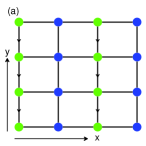
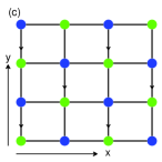
Figure S1: Schematic of the lattices. Here, the green and blue balls represent the lattice sites of sublattices $A$ and $B$, respectively. The arrows represent the hopping-accompanying phase. (a) Model 1: the hopping-accompanying phase is $0<\gamma<2\pi$: (b) Model 2: the hopping-accompanying phases are $0<\beta<\pi$ in the $x$ direction and $0<\gamma<\pi$ in the $y$ direction; and (c) Model 3: the hopping-accompanying phase is $0<\gamma<2\pi$.

Table S1: Summary of three models with hidden symmetry-protected degeneracy

Model	Primitive lattice vectors	Primitive reciprocal lattice vectors	Symmetry operator	The effect of symmetry acting on wave vectors	Symmetry-invariant points	Symmetry-protected degenerate points
1	${\bm{a}}_{1}=(2,0)$, ${\bm{a}}_{2}=(0,1)$	${\bm{b}}_{1}=(\pi,0)$, ${\bm{b}}_{2}=(0,2\pi)$	$\Upsilon=(e^{i\gamma})^{i_{y}}\sigma_{x}KT_{{\bm{a}}_{1}/2}$,                $\Upsilon^{2}=T_{{\bm{a}}_{1}}$	$\Upsilon:(k_{x},k_{y})\rightarrow(-k_{x},\gamma-k_{y})$	$(\pi/2,\gamma/2)$, $(\pi/2,\gamma/2-\pi)$,                                                  $(0,\gamma/2)$, $(0,\gamma/2-\pi)$	$(\pi/2,\gamma/2)$, $(\pi/2,\gamma/2-\pi)$
2	${\bm{a}}_{1}=(2,0)$, ${\bm{a}}_{2}=(0,1)$	${\bm{b}}_{1}=(\pi,0)$, ${\bm{b}}_{2}=(0,2\pi)$	$\Upsilon=(e^{2i\beta})^{i_{x}}\sigma_{x}KT_{{\bm{a}}_{1}/2}$, $\Upsilon^{2}=e^{2i\beta}T_{{\bm{a}}_{1}}$	$\Upsilon:(k_{x},k_{y})\rightarrow(2\beta-k_{x},-k_{y})$	$(\beta-\pi/2,0)$, $(\beta-\pi/2,\pi)$, $(\beta,0)$, $(\beta,\pi)$	$(\beta-\pi/2,0)$,                $(\beta-\pi/2,\pi)$
3	${\bm{a}}_{1}=(1,1)$, ${\bm{a}}_{2}=(1,-1)$	${\bm{b}}_{1}=(\pi,\pi)$, ${\bm{b}}_{2}=(\pi,-\pi)$	$\Upsilon=(e^{i\gamma})^{i_{y}}\sigma_{x}KT_{({\bm{a}}_{1}+{\bm{a}}_{2})/2}$, $\Upsilon^{2}=T_{{\bm{a}}_{1}+{\bm{a}}_{2}}$	$\Upsilon:(k_{x},k_{y})\rightarrow(-k_{x},\gamma-k_{y})$	$(-\pi/2,\gamma/2-\pi/2)$, $(\pi/2,\gamma/2-\pi/2)$, $(0,\gamma/2)$, $(0,\gamma/2-\pi)$	$(-\pi/2,\gamma/2-\pi/2)$, $(\pi/2,\gamma/2-\pi/2)$

Note: Here, $i_{x}$ and $i_{y}$ are the $x$ and $y$ components of the coordinate $i$ of lattice sites, respectively.

In order to show the ubiquity of symmetry-protected isolated point degeneracies, we show three other models as shown in Fig.S1 in this Supplementary Material. Here, for brevity, we assume the distance between the two neighbor lattice sites $d=1$. All the lattices considered here consist of two sublattices marked by blue and green balls in Fig.S1. In all the models, hopping between neighbor sites is allowed and the hopping amplitudes are the same. For some hoppings between neighbor sites, there exist hopping-accompanying phases, which are represented by arrows in Fig.S1. The magnitudes of hopping-accompanying phase represented by arrows are (i) $0<\gamma<2\pi$ in the $y$ direction for Model 1, (ii) $0<\beta<\pi$ in the $x$ direction, $0<\gamma<\pi$ in the $y$ direction for Model 2, (iii) $0<\gamma<2\pi$ in the $y$ direction for Model 3, respectively. The corresponding primitive lattice vectors, primitive reciprocal lattice vectors, symmetry operator, the transformation of wave vector under symmetry operation, symmetry-invariant points in the Brillouin zone, and symmetry-protected degenerate points are summarized in Table S1.

References

• (1) M.Z. Hasan and C.L. Kane, Rev. Mod. Phys. 82, 3045 (2010).
• (2) X.L. Qi and S.C. Zhang, Rev. Mod. Phys. 83, 1057 (2011).
• (3) A.P. Schnyder, S. Ryu, A. Furusaki, and A.W.W Ludwig, Phys. Rev. B 78, 195125 (2008); ibid. AIP Conf. Proc. 1134, 10 (2009); A. Kitaev, AIP Conf. Proc. 1134, 22 (2009).
• (4) D.J. Thouless, M. Kohmoto, M.P. Nightingale, M. den Nijs, Phys. Rev. Lett. 49, 405 (1982).
• (5) F.D.M. Haldane, Phys. Rev. Lett. 61, 2015 (1988).
• (6) X.J. Liu, X. Liu, C. Wu, and J. Sinova, Phys. Rev. A 81, 033622 (2010).
• (7) C.L. Kane, E.J. Mele, Phys. Rev. Lett. 95, 226801 (2005); ibid. 95, 146802 (2005).
• (8) N. Read and D. Green, Phys. Rev. B 61, 10267 (2000).
• (9) X.L. Qi, T.L. Hughes, S. Raghu, and S.C. Zhang, Phys. Rev. Lett. 102, 187001 (2009).
• (10) X. Wan, A.M. Turner, A. Vishwanath, and S.Y. Savrasov, Phys. Rev. B 83, 205101 (2011).
• (11) G. Xu, H. Weng, Z. Wang, X. Dai, and Z. Fang, Phys. Rev. Lett. 107, 186806 (2011).
• (12) A.A. Burkov, M.D. Hook, and L. Balents, Phys. Rev. B 84, 235126 (2011).
• (13) A.A. Burkov and L. Balents, Phys. Rev. Lett. 107, 127205 (2011).
• (14) C. Fang, M.J. Gilbert, X. Dai, and B.A. Bernevig, Phys. Rev. Lett. 108, 266802 (2012).
• (15) A.A. Zyuzin, S. Wu, and A.A. Burkov, Phys. Rev. 85, 165110 (2012).
• (16) K. Sun, W.V. Liu, A. Hemmerich and S. Das Sarma, Nat. Phys. 8, 67 (2012).
• (17) J.H. Jiang, Phys. Rev. A 85, 033640 (2012).
• (18) P. Hosur, S.A. Parameswaran, and A. Vishwanath, Phys. Rev. Lett. 108, 046602 (2012).
• (19) P. Delplace, J. Li, and D Carpentier, Europhys. Lett. 97, 67004 (2012).
• (20) C. Herring, Phys. Rev. 52, 365 (1937).
• (21) L. Balents, Phys. 4, 36 (2011).
• (22) L.K. Lim, C. M. Smith, and A. Hemmerich, Phys. Rev. Lett. 100, 130402 (2008).
• (23) J.M. Hou, W.X. Yang and X.J. Liu, Phys. Rev. A 79, 043621 (2009).
• (24) N. Goldman, A. Kubasiak, A. Bermudez, P. Gaspard, M. Lewenstein, and M. A. Martin-Delgado, Phys. Rev. Lett. 103, 035301 (2009).
• (25) D. Bercioux, D. F. Urban, H. Grabert, and W. Häusler, Phys. Rev. A 80, 063603 (2009).
• (26) N. Goldman, E. Anisimovas, F. Gerbier, P. Öhberg, I. B. Spielman, G. Juzeliūnas, New J. Phys. 15, 013025 (2013).
• (27) See Supplemental Material for details.
• (28) C. Bena and G. Montambaux, New J. Phys., 11, 095003 (2009).
• (29) I. Bloch, J. Dalibard, and W. Zwerger, Rev. Mod. Phys. 80, 885 (2008).
• (30) Y.J. Lin, R.L. Compton, K. Jiménez-García, J.V. Porto, and I.B. Spielman, Nature, 462, 628 (2009).
• (31) M. Aidelsburger, M. Atala, S. Nascimbène, S. Trotzky, Y.A. Chen, and I. Bloch, Phys. Rev. Lett. 107, 255301 (2011).
• (32) D.A. Abanin, T. Kitagawa, I. Bloch, and E. Demler, Phys. Rev. Lett. 110, 165304 (2013).
• (33) E. Alba, X. Fernandez-Gonzalvo, J. Mur-Petit, J.K. Pachos, and J.J. Garcia-Ripoll, Phys. Rev. Lett. 107, 235301 (2011).
• (34) X.J. Liu, K.T. Law, T.K. Ng, and P.A. Lee, arXiv:1306.5223.

References

• (1) C. Bena and G. Montambaux, New J. Phys. 11, 095003 (2009).
• (2) C. Fang, M.J. Gilbert, X. Dai, and B.A. Bernevig, Phys. Rev. Lett. 108, 266802 (2012).