Thermal Correlators in the channel of two-flavor QCD
Bastian B. Brandtb,c, Anthony Francisb,d, Harvey B. Meyera,b,d and Hartmut Wittiga,b,d
a PRISMA Cluster of Excellence, Johannes Gutenberg-Universität Mainz, D-55099 Mainz b Institut für Kernphysik, Johannes Gutenberg-Universität Mainz, D-55099 Mainz c Institut für theoretische Physik, Universität Regensburg, D-93040 Regensburg d Helmholtz Institut Mainz, Johannes Gutenberg-Universität Mainz, D-55099 Mainz
Abstract
We present a lattice QCD calculation with two dynamical flavors of the isovector vector correlator in the high-temperature phase. We analyze the correlator in terms of the associated spectral function, for which we review the theoretical expectations. In our main analysis, we perform a fit for the difference of the thermal and vacuum spectral functions, and we use an exact sum rule that constrains this difference. We also perform a direct fit for the thermal spectral function, and obtain good agreement between the two analyses for frequencies below the two-pion threshold. Under the assumption that the spectral function is smooth in that region, we give an estimate of the electrical conductivity.
PACS: 12.38.Gc, 11.10.Wx, 12.38.Mh, 25.75.Cj
Keywords:
Lattice QCD, Thermal Field Theory, Quark-Gluon Plasma, Lepton production
1 Introduction
The properties of strongly interacting matter under extreme conditions are the subject of intensive experimental and theoretical investigation. A comprehensive picture of a state of matter requires not only the knowledge of equilibrium properties such as the equation of state and static susceptibilities, but also an understanding of its transport properties.
In the high-temperature phase of QCD, the transport coefficients (the shear and bulk viscosities as well as the electrical conductivity) have been calculated perturbatively to full leading order in the strong coupling [1, 2, 3]. However, in the range of temperatures that can be reached in heavy ion collisions, the perturbative uncertainty remains large. Phenomenologically, the observation of large elliptic flow in heavy ion collisions at RHIC and at the LHC hints at a small shear viscosity ([4, 5] and references therein). Furthermore, the measured spectrum of dileptons is related to the spectral functions of the electromagnetic current, integrated over the history of the expanding system [6].
Any reliable calculation of a transport coefficient of QCD at a temperature of a few hundred MeV would be extremely valuable. It therefore makes sense to undertake a calculation in the comparatively easiest possible channel. For a lattice QCD approach, the spectral function of the isovector vector current is perhaps the most accessible channel. First, the correlation function is evaluated via a single, connected Wick contraction, allowing for a good signal-to-noise ratio in the Monte-Carlo simulation. Second, the light quarks do not introduce a new dynamical scale into the problem in the way that heavy quarks do, which typically requires the use of an effective field theory. Third, the corresponding vacuum spectral function, being extremely well known experimentally due to decades of measurements of the ratio and of decays (see for instance [7]), provides a useful reference.
Here we present the first lattice calculation of the Euclidean isovector vector correlator in the high-temperature phase of QCD with dynamical quark flavors and analyze it in terms of the spectral function. We adopt an approach used previously in the bulk channel [8], which consists in analyzing directly the difference of the thermal and vacuum correlators. Moreover, we exploit a recently derived sum rule which constrains the integral over the difference of spectral functions (divided by frequency) to vanish. We compare our results at finite lattice spacing with a recent analysis performed in the continuum limit of quenched QCD [9].
In spite of the technically favorable properties of the channel, determining the vector spectral function with frequency resolution remains a numerically ill-posed problem (see for instance the discussion in [10]). Our main goal in this paper is therefore of qualitative nature and consists in determining the gross features of the thermal spectral function, in particular in which frequency bins (of width ) it under- or overshoots the vacuum spectral function.
2 Theoretical expectations for the spectral function
In this section we set up our notation and define the relevant correlation functions. We summarize the theoretical expectations for these correlators and the associated transport properties.
2.1 Definitions
Our primary observables are the Euclidean vector current correlators,
| (2.1) |
with the isospin current. The expectation values are taken with respect to the equilibrium density matrix , where is the inverse temperature. The quark number susceptibility is defined as
| (2.2) |
Due to charge conservation, the two correlators of interest are exactly related via
| (2.3) |
The Euclidean correlators have the spectral representation
| (2.4) |
For a given function , the reconstructed correlator is defined as
| (2.5) |
It can be interpreted as the Euclidean correlator that would be realized at temperature if the spectral function was unchanged between temperature and . For it can be directly obtained from the zero-temperature Euclidean correlator via [8]
| (2.6) |
2.2 Theoretical predictions
The isospin diffusion constant is given by a Kubo formula in terms of the low-frequency behavior of the spectral function,
| (2.7) |
In the thermodynamic limit, the subtracted vector spectral function obeys a sum rule (see [11] sec. 3.2),
| (2.8) |
This sum rule is based on two ingredients. Firstly, the two-point function of a spatial component of the vector current at vanishing four-momentum can be interpreted as the susceptibility of the isospin charge at zero temperature in a system with one short spatial periodic dimension of length . As long as the correlation lengths are finite, this susceptibility vanishes. Secondly, subtracting the same quantity in the infinite-volume vacuum enables one to write a convergent sum rule in for the susceptibility. It is well known from the operator-product expansion that the difference of spectral functions in Eq. (2.8) falls off as at large frequencies, see [12, 13] for explicit calculations.
For non-interacting massive quarks in the fundamental representation of the SU() color group, the vector spectral function is diagonal in flavor space and takes the form
The next-to-leading order has been computed very recently [14]. At large frequencies the radiative corrections to the coefficient of the term are temperature independent and known to order [15] (for quark mass effects in the vacuum, see [16]). The susceptibility and the mean squared transport velocity have the following expressions,
| (2.10) | |||||
| (2.11) |
with the Fermi-Dirac distribution and . It is now straightforward to check that the sum rule (2.8) is verified in the free theory. The positive contribution of the transport peak (the contribution in the free theory) is compensated by a deficit of the thermal spectral function at intermediate frequencies, in the massless case. The susceptibility and mean square velocity have simple expressions in the massless and in the heavy-quark limits,
|
(2.12) |
Beyond the non-interacting theory, at weak coupling kinetic theory predicts the presence of a narrow transport peak in the spectral function at , whose width and height are related to the properties of the quasi-particles. Introducing a separation scale between the transport time scale and the thermal time-scale, the area under the transport peak is, to leading order, preserved by the interactions [17],
| (2.13) |
The width of the transport peak however becomes finite. In the heavy-quark limit for instance, the Langevin effective theory predicts a Lorentzian form [17]
| (2.14) |
where is the ‘drag coefficient’, . The case of massless quarks can be treated with the Boltzmann equation [1, 18, 19], with a form of the spectral function qualitatively similar to Eq. (2.14) and a drag coefficient given by
| (2.15) |
with the Debye mass and .
Finally, in contrast with the weak-coupling analysis outlined above, it is worth mentioning that at least one theory is known where the vector spectral function does not exhibit a transport peak. In the strongly coupled super-Yang-Mills theory, the spectral function of the R-charge correlator reads [20],
| (2.16) |
The static susceptibility is given by , and the diffusion constant by .
2.3 Connection with electromagnetic observables
The electrical conductivity is extracted from the correlator of the current . If the quark species are degenerate, this correlator is given by the sum of a contribution proportional to and a contribution proportional to . At high frequencies, the latter contribution to the spectral function is predicted to be small in perturbative QCD. Assuming that this contribution is also small at low frequencies, we have for the electrical conductivity in QCD
| (2.17) |
with . If one further assumes that is fairly insensitive to the quark mass, and that the transport properties are not significantly affected by the presence of virtual strange quark pairs, the electrical conductivity in QCD is given by Eq. (2.17) with .
2.4 Phenomenology of the resonance
In the vacuum, the QCD spectral function of the electromagnetic current is well measured via the ratio. The meson completely dominates the spectral function up to about . We work in the exact isospin symmetric theory and therefore ignore issues related to isospin breaking and mixing, see [22] for a recent reference.
Since we are working with the isospin current, we should restrict ourselves to final hadronic states with . The ratio is defined analogously to with this restriction. A rough parametrization of the experimentally measured ratio was given in Ref. [11], Eq. (93). The spectral function in our normalization is related to the ratio via
| (2.20) |
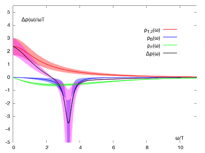
We can now make a simple argument about the thermal spectral function based on the exact sum rule (2.8), the kinetic theory sum rule (2.13) and the experimentally known vacuum spectral function. Using the parametrization of [11], the area under the vacuum spectral function up to is about
| (2.21) |
By contrast, the corresponding area for free massless quarks at zero temperature is
| (2.22) |
Taking into account the physical light quark masses changes this value by a negligeable amount.

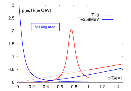
In the free theory, the sum rule (2.8) is satisfied. Now switching on interactions between quarks, let us assume for the sake of the argument that in the high temperature phase they can be described perturbatively. In the small frequency region, interactions turn the delta function in Eq. (2.2) into an approximate Lorentzian curve [18], preserving its area to leading order. This is the content of a kinetic theory sum rule [17]. In the vacuum, interactions have a dramatic effect on the spectral function, due to chiral symmetry breaking and confinement, and convert its area up to 1GeV from to . Since the sum rule (2.8) must still be satisfied, the weak-coupling spectral function in the high-temperature phase must acquire an additional area of
| (2.23) |
Note that at very high temperatures, the area (2.23) is negligible compared to the area under the transport peak, which grows as . However, consider the situation at (the temperature at which we have computed the correlator on the lattice, see the next section). Assuming the existence of a transport peak, its area is about , if we correct for the fact that the static isospin susceptibility is about below its Stefan-Boltzmann limit (see table 1 and [23]). The area missing from the weak-coupling spectral function is thus comparable in size to the transport peak area at this temperature. The argument is illustrated in Fig. (1).
At , the difference of spectral functions can be analyzed with the operator product expansion (see [13, 24] and References therein). The lowest-dimensional gauge-invariant operators are of dimension four, and therefore the asymptotic behavior is (possibly up to logarithms). According to Eq. (4.1) of Ref. [24], the leading term of order is positive. However, at its contribution to the area under is too small to explain the missing area (2.23).
In conclusion, at temperatures that are accessible in heavy-ion collisions, the sum rule (2.8) and the ratio measurements place an important constraint on the thermal spectral function.
3 Lattice QCD data
All our numerical results were computed on dynamical gauge configurations with two light, mass-degenerate -improved Wilson quark flavors. The configurations were generated using the MP-HMC algorithm [25, 26] in the implementation of Marinkovic and Schaefer [27] based on Lüscher’s DD-HMC package [28]. The zero-temperature ensemble was made available to us through the CLS effort [29]. The gauge action is the standard Wilson plaquette action [30], while the fermions were implemented via the Wilson-Clover discretization with non-perturbatively determined clover coefficient [31].
We calculated correlation functions using the same discretization and masses as in the sea sector in two different ensembles. The first corresponds to virtually zero-temperature on a lattice (labeled O7 in [32]) with a lattice spacing of fm [32] and a pion mass of MeV, so that . Secondly we generated an ensemble on a lattice of size with all bare parameters identical to the zero-temperature ensemble. In this way it is straightforward to compare the correlation functions respectively in the confined and deconfined phases of QCD. Choosing yields a temperature of MeV. Based on preliminary results on the pseudo-critical temperature of the crossover from the hadronic to the high-temperature phase [33], the temperature can also be expressed as .
The renormalization of the vector correlator assumes the form
| (3.24) |
The dots refer to O() contributions from the improvement term proportional to the derivative of the antisymmetric tensor operator [34, 35] that we did not compute. We note however that perturbatively, the O() contribution is suppressed by two powers of . We use the non-perturbative value of provided by [36]. From the perturbative results of [35] we estimated the magnitude of the term to be of the order of . Considering that the error of is at the level, we drop this contribution altogether in the following. Note that since we use the same bare parameters at zero and finite temperature, the multiplicative renormalization of the vector current only affects the corresponding correlation functions – and their difference – by an overall factor.

The vacuum correlator serves as a reference in this work. To fix the parameters of the lightest vector state in the finite volume of the simulation, we fitted the vacuum correlation function to an Ansatz of the form
| (3.25) |
which is the Laplace transform of
| (3.26) |
The finite-volume spectral function consists of Dirac functions. However, since many states contribute at short distances, the continuum in Eq. (3.25) should be interpreted as resulting from the contributions of many energy eigenstates. In Fig. 2 we show the vacuum vector correlator and the fit result. The insert shows the corresponding effective mass. The fit (performed in the interval ), clearly provides a good description of the data. For the quality of the data deteriorates and the signal is lost.
We will only use the result for the parameters and in the following. The question arises of the relation of these parameters to the infinite-volume spectral function. An answer is given by Refs. [37, 38]. Assuming phenomenologically reasonable values of the coupling to the channel, the mass in fact appears to be within of the (infinite-volume) mass [37].
In addition we estimate the thermal (isovector) quark number susceptibility from the time-time component of the vector correlation function (see Eq. 2.2), by reading off the midpoint of the time-time correlator. We checked the obtained value by fitting the correlator to a constant in the region and found only a negligible deviation. The parameters used in our lattice setup, the ‘-meson’ parameters and the value of the static susceptibility are summarized in Tab. 1.
| Ref. | |||
| 5.50 | |||
| 0.13671 | |||
| 1.7515 | |||
| 0.768(5) | [36] | ||
| 0.0486(4)(5) | [32] | ||
| [MeV] | 270 | [32] | |
| 253(4) | |||
| 0.871(1) | |||
| 4.42(31) | |||
| 3.33(5) | |||
| 1.244(5) | |||
| 5.98(11) | |||
3.1 Thermal and vacuum correlators
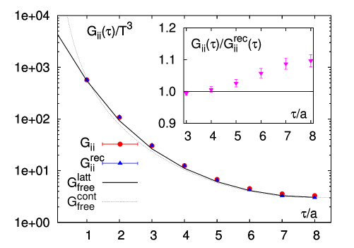
In Fig. 3 we show the correlator computed at MeV together with the corresponding free ‘continuum’ and free ‘lattice discretized’ correlation functions. In addition we show the reconstructed correlator as obtained from Eq. 2.6. The results for the thermal and reconstructed correlators for can be found in Tab. 2.
The reconstructed correlator lies somewhat lower than the thermal correlator. The insert in Fig. 3 displays the ratio in order to make their relative dependence visible. For small Euclidean times this ratio is unity, above it increases monotonically until it levels off around the midpoint at about above unity. A thermal modification of the spectral function has thus taken place (recall that the spectral function underlying contains the bound states of the confined theory).
| 4 | 12.534(94) | 12.456(59) |
|---|---|---|
| 5 | 6.775(65) | 6.602(41) |
| 6 | 4.510(51) | 4.264(35) |
| 7 | 3.569(45) | 3.282(33) |
| 8 | 3.300(44) | 3.008(34) |
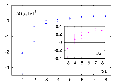
In Fig. 4 we show the difference
| (3.27) |
of the thermal and the reconstructed correlators. Given that and have the same behavior, this means we are subtracting non-perturbatively the ultraviolet tail of the spectral function. Using this difference we are therefore able to probe the change in the vector spectral function from the confined to the deconfined phase for frequencies .
For small times, the difference (3.27) turns out to be negative, while it is positive for . Note the errors decrease with increasing Euclidean time throughout the available range. We show a more detailed view of the region in the insert of Fig. 4. Here the difference still exhibits a mild increase and levels off near the midpoint. The value it reaches at the midpoint is .
3.2 Comparison with the free-quark correlator
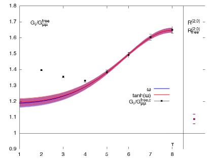
In the previous subsection we compared the thermal correlator to its zero-temperature analogue. Now we analyze the thermal correlator in relation to the non-interacting case, which by asymptotic freedom corresponds to the regime of asymptotically high temperature. However, before discussing the departure of the simulation data from the non-interacting case, we address briefly the issue of cutoff effects.
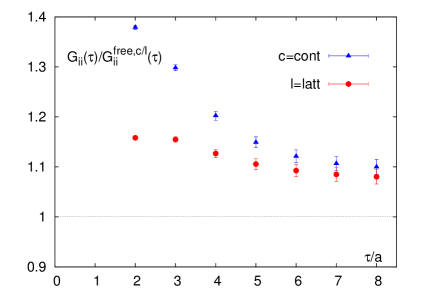
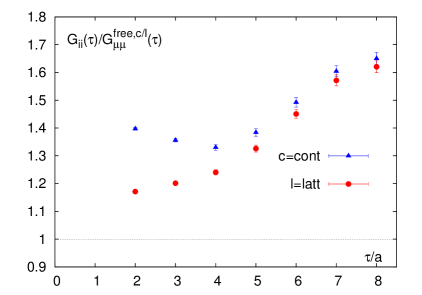
Since we only have data at one lattice spacing, the value of the lattice correlator, viewed as an estimator of the continuum correlator, is necessarily ambiguous at some level due to cutoff effects. To estimate the size of this ambiguity, we show the ratio in Fig. 5(left), where and denote the analytically known free continuum and free lattice cases, respectively [39]. Concentrating on the ratio to the free continuum correlator we observe a decreasing trend throughout the entire available Euclidean time range, a behavior very similar to that seen in quenched studies [9]. Taking the ratio to the free lattice correlation function on the other hand the results are much flatter and almost constant at small times , while for the two ratios track each other and are separated by a small shift of roughly . The difference between the two curves comes from the fact that the free lattice correlation function takes into account the tree-level lattice artifacts.
To put this systematic uncertainty into perspective, we examine the ratio in the right panel of Fig. 5. The only difference between and is that the -function in the spectral function at is absent in the latter. The difference between the left and right panel curves thus corresponds to the contribution of the transport peak. It is clear from the figure that this contribution is much larger than the cutoff effects present at tree-level for .
Returning now to the question of how much the thermal correlator differs from its non-interacting counterpart, we see that the simulation data lies 8 to 10 above the free lattice correlator. The sign of the effect corroborates our finding in section 2.4 that spectral weight is missing from the weak coupling spectral function.
3.3 Thermal moments of the correlator
Finally we compute also the ratio of thermal moments of the correlator [9]:
| (3.28) |
This quantity can be extracted from the correlator data by combining the results of and:
| (3.29) |
In the free case a straightforward computation [40] yields . Using this result together with our lattice data we obtain:
| (3.30) |
where we neglected higher-order terms in the square bracket of Eq. (3.29)111Including the leading correction into a fit we find it to be poorly determined by the data, while the constant contribution remained unchanged within errors.. We see that the ratio of thermal moments is roughly larger than the free result. As the ratio of second thermal moments is sensitive to changes in the low frequency region of the spectral function (see e.g. [9]), this observation could be due to a broadening of the -function form of the free theory.
4 Analysis of lattice correlators in terms of spectral functions
We begin with a simple but instructive analysis of the spectral function difference . Section 4.2 contains the main analysis based on fits to the thermal part of the Euclidean correlator, and section 4.3 describes a fit directly to the thermal correlator. The results of the two fits are compared against each other and against previous quenched calculations in section 4.4.
4.1 A simple spectral analysis of the thermal part of the vector correlator
Based on the analysis of section 2.4, it is interesting to ask whether the Euclidean correlator can be described and the sum rule (2.8) satisfied solely by the transport peak and the -meson contribution. For this purpose, we consider the following caricature of , where the sum rule has already been enforced,
| (4.31) |
corresponding to the Euclidean correlator
| (4.32) |
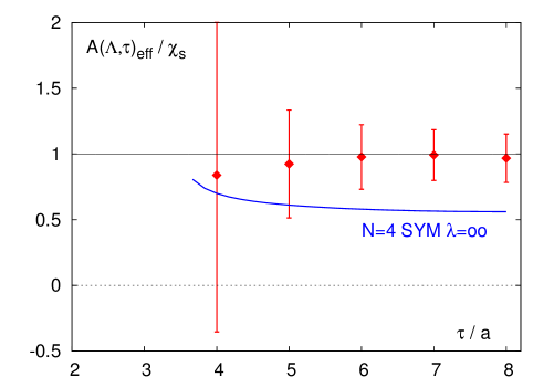
The mass is set equal to the value obtained by fitting the Ansatz (3.25) to the vacuum correlator and given in table 1. The kinetic theory sum rule (2.13) implies that is an estimator for , and from Eq. (4.32) an effective value can thus be defined for every value of ,
| (4.33) |
The result is shown in Fig. (6). The quantity is well compatible with a constant value, implying that the Ansatz (4.31) already provides a good description of the lattice correlator. Moreover, the weak-coupling expectation that should be given by (up to quark mass effects reducing their average thermal velocity ) is also well reproduced.
It should be noted that in this simple picture the prefactor of in Eq. (4.31) is about , to be compared with the area obtained from the vacuum correlator (table 1). This observation means that the area under the thermal spectral function in the region cannot be negligible compared to , confirming the conclusions drawn from phenomenology in section (2.4).
It is interesting to confront the lattice data with the spectral function in the strongly coupled SYM theory, Eq. (2.16). We therefore also plot the corresponding SYM function in Fig. (6). It lies lower than the lattice data, in spite of the fact that has the same large-frequency limit as in QCD and also satisfies the sum rule (2.8). This comparison shows that the lattice data is not simultaneously compatible with the combination of (a) the functional form of the SYM spectral function and (b) the corresponding very low diffusion constant. The data is however perfectly compatible with the substitution of the delta function in Eq. (4.31) by a flat (or even as in the SYM case) behavior of up to about , provided its area is adjusted appropriately.
In order to parametrize systematically, including the expected contributions at high frequencies, we resort to the more sophisticated fits described in the next subsection. To anticipate the results, similar qualitative conclusions on the distribution of the spectral weight in will be obtained.
4.2 Fit to the thermal part of the vector correlator
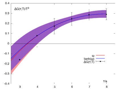
We proceed to investigate the behavior of the thermal part of the spectral function by fitting the difference of the thermal and the reconstructed correlator, see Eq. (3.27). We know from the operator-product expansion that the difference of spectral functions falls off rapidly (as ) for , and therefore focus on the region in order to choose a fit Ansatz. As described in the previous subsection, the fact that the data (displayed in Fig. 4) is positive at long distances and negative at short distances suggests that the thermal spectral weight exceeds the vacuum spectral weight at low frequencies and falls short of it at higher frequencies222A continuum extrapolation is really needed to confirm the behavior at short distances..
We thus parametrize using the following Ansatz for :
| (4.34) | |||||
| (4.35) | |||||
| (4.36) | |||||
| (4.37) |
The bound state (B) and the transport peak (T) are represented by Breit-Wigner forms. Even such a simple Ansatz requires three parameters to determine the bound state peak, two parameters for the transport peak and one for the ‘perturbative’ contribution (F). We will therefore fix some of them using the vacuum correlator. In the following we set equal to , given in Tab. 1, which we obtained from the exponential fit to the vacuum correlator. Note that the area under the bound state peak does not depend on the width in the limit where it is small. The sensitivity of the Euclidean correlator to the latter parameter is very small. We therefore perform fits for three fixed values of this parameter, and check the sensitivity of the result. We choose the values and 1.0, corresponding to and 250MeV.

The tail of the Ansatz violates the OPE prediction that at large frequencies. It has been argued in [41] that this might lead to an overestimate of the transport contribution. To avoid this problem we introduce the Ansatz 2, where . This Ansatz possesses the correct asymptotic behavior, as well as the expected linear behavior in at small frequencies.
Finally, to complete the parametrization of , we include a weak-coupling term inspired by Eq. (2.2) describing the subtraction of the large frequency parts of the thermal and vacuum spectral functions. This contribution vanishes exponentially as the frequency increases.
In the next step we fit the combined Ansätze of to the data, while at the same time satisfying the sum rule of Eq. 2.8 to an accuracy of . We limit ourselves to fitting the region only, in order to minimize the influence of cut-off effects, as discussed in Sec. 3.1. With determined by the vacuum correlator, we set successively to the three different values mentioned above and fixed around unity, and fitted the parameters , and . The errors and error bands shown in the following have been computed using the covariance matrix of the corresponding fit for fixed values of and .
The resulting correlators and spectral functions are displayed in Fig. 7 for and while the fitted parameters are given in Tab. 3. In the left panel of Fig. 7 the data is compared to the fits using and as transport contribution. We achieve a quasi-perfect description of the data for . The right panel shows that both Ansätze exhibit a substantial spectral weight around the origin and a negative contribution from the region of the mass.
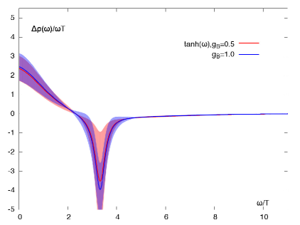
Focussing on Ansatz 2, the left panel of Fig. 8 shows the sensitivity of the fit result to varying the parameter . Varying the width only has a small effect on the overall result. We also found little sensitivity to variations in . In order to understand what drives the parameters to their final fitted values, we also plot separately the three contributions appearing in Eq. (4.34–4.37), including their respective error bands, in the right panel of Fig. 8. The contribution mainly affects the intermediate frequency region around . Its tail between is largely compensated by the tail of the Lorentzian centered at the origin, and this might well be what drives the width of the Lorentzian.
4.3 Weak-coupling inspired fit to the thermal vector
In contrast to the previous section, here we study directly the thermal vector correlator and its ratio of thermal moments . We perform a fit inspired by the weak coupling form of the thermal spectral function,
| (4.38) |
where the form of the two contributions is defined in Eq. (4.36) and (4.37). At a given temperature this Ansatz is characterized by three parameters . We fit the full Ansatz to the thermal correlator , while at the same time demanding that be reproduced. In this analysis the three parameters and are fitted, and the fit range is as before.
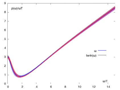
The resulting correlators and spectral functions are shown in Fig. 9 with their fit parameters listed in Tab. 3. The ratio in the left panel of Fig. 9 is well described by both versions and of the transport contribution for , while also the ratio of thermal moments (given on the far right of the plot) is reproduced. For our Ansatz fails to reproduce these points, which we suspect is partly due to cutoff effects. In the future it would be interesting to repeat the calculation at several smaller lattice spacings while keeping the temperature fixed, as in [9].
On the right hand side of Fig. 9 we show the resulting spectral functions divided by . Clearly both Ansätze give very similar results that lie within errors of each other. The thermal correlator is even less sensitive to the asymptotic behavior of the transport contribution in the Ansatz than in the difference of correlators studied in Sec. 4.2.
4.4 Discussion
| 0.61(10) | 1.22(26) | 1.42(188) | 0.702(201) | 0.806(231) | |
| 0.59(16) | 5.7(10) | 2.92(228) | 0.764(244) | 0.877(280) | |
| 0.75(4) | 0.71(9) | 1.186(27) | 0.818(50) | 0.939(57) | |
| 0.74(5) | 0.98(13) | 1.192(26) | 0.858(56) | 0.985(64) |
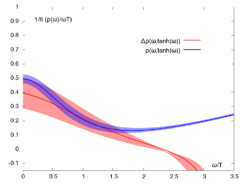
We now compare the results of the fits to and . Since the vacuum spectral function vanishes below (in infinite volume), and should be equal for . We thus plot the spectral functions obtained from the two fits in this frequency region, see Fig. 10. Here we restrict ourselves to showing these results based on , as their theoretical foundation is more sound than those with . All curves are multiplied by a factor , which means that the intercept at yields an estimate of with the electrical conductivity of the quark gluon plasma.
The results obtained by fitting agree very well with the central values obtained by fitting , as summarized in Tab. 3. The fit to using the transport Ansatz yields a slightly lower intercept. If we assume the spectral function to be as smooth around the origin as Fig. 10 suggests, we obtain the following estimate for the electrical conductivity of the quark gluon plasma at MeV,
| (4.39) |
where for and for , see Sec. 2.3. It should be remembered that the Euclidean correlator can be perfectly well described by an infinitely narrow transport peak (corresponding to an infinite electrical conductivity), see section 4.1. Although obtained under a strong assumption, it is interesting to compare (4.39) to other lattice results obtained under similar assumptions. The following comparison is made with quenched results, since to our knowledge there are no previous dynamical QCD studies.
A quenched calculation using staggered fermions based on fitting the Fourier transform of the correlator obtained [42] at , where the pure SU(3) gauge theory critical temperature is around 290 MeV. A further study using staggered fermions and an analysis based on the maximum entropy method obtained [43]. Finally, a recent quenched study using Wilson-Clover fermions in the continuum limit obtained at [9]. Our results using dynamical Wilson-Clover fermions at are thus completely compatible with the recent quenched results.
Even though the transport contribution extracted from our fits is not narrow and an interpretation in terms of kinetic theory (Eq. 2.13) is no longer rigorously motivated, we also compute the effective mean squared velocity of the quarks . Choosing the scale parameter and numerically integrating the fitted spectral functions we obtain . Assuming Eq. (2.13) and using the quark number susceptibility as given in Tab. 1, it is straightforward to estimate an effective mean squared velocity . The results for and are listed in Tab. 3. For all fits we obtain reasonable values for in the range . Thus, although we are not able to demonstrate or exclude the validity of the kinetic theory description, the values of the effective quark velocity extracted in this way are in line with its expectations. By contrast, the AdS/CFT spectral function (2.16) (which clearly cannot be described by kinetic theory) yields an effective quark velocity of for .
Using the result for from the fit to , it is straightforward to compute the production rate of thermal lepton pairs in the quark gluon plasma with two light dynamical quark flavors from Eq. (2.18). The resulting rates are shown in Fig. 11. We give the low frequency behavior of obtained from using the Ansatz 2 in the transport region. Comparing our results with the free (Born) rate (dashed line) and the hard thermal loop result (black line) with a thermal mass of [44], we observe that for frequencies our result is below the result from HTL, above this value however it follows it very closely.
The results shown in Fig. 11 correspond to a system at thermal equilibrium with MeV. To make contact with results obtained in heavy ion collisions one has to take into account the real-time evolution of the volume of the system, using a hydrodynamic model along the lines of [45] (for a recent study of out-of-equilibrium photon and dilepton production using the AdS/CFT correspondence see [46, 47]).

5 Conclusion
In this paper we have obtained the isovector vector correlator in the high-temperature phase of two-flavor QCD at MeV as well as in the vacuum at the same set of bare parameters. This allowed us to analyze both the difference of the thermal and the vacuum correlator and the thermal correlator directly. In the former case the analysis is further constrained by an exact sum rule. Given the uncertainties inherent in trying to extract information on the spectral function from Euclidean correlators, the two methods give a consistent picture of the thermal spectral function in the low to moderate frequency range .
The vacuum spectral function is known to receive a very large contribution from the meson from experimental and decay data. The main qualitative lesson we have learnt is that the reduction or complete absence of such a peak and the appearance of a substantial spectral weight in the low-frequency region provide a very good description of the lattice data and are compatible with the sum rule. Moreover the area under the latter spectral weight matches the expectation of kinetic theory. This picture is corroborated by a simple phenomenological study, presented in section 2.4, based on the experimental ratio and the sum rule. We also note that the analytic result (2.16) in the strongly coupled limit of super-Yang-Mills theory exhibits a qualitatively similar (but quantitatively different in amplitude) change of sign in the difference of thermal and vacuum spectral functions, even though the theory is conformal and therefore exhibits no analogue of the meson. A similar pattern was also observed in the bulk channel of the pure SU(3) gauge theory [8].
The analysis presented in this paper is based on data at finite lattice spacing. Obviously the next step would be to repeat the analysis in the continuum limit, as has been done in the quenched theory [48]. In this respect the results obtained here should be regarded as preliminary. We note however that our results are quantitatively quite close to those obtained in [48].
It would be very interesting to repeat the analysis carried out here in a temperature scan through the smooth phase transition. This would allow one to track the fate of the meson from the low-temperature to the high-temperature phase and perhaps to shed light on the excess of dileptons observed by the PHENIX collaboration in relativistic gold-gold collisions [49]. The methods employed here to constrain thermal spectral functions may be useful in the context of cosmology as well, see for instance [50].
Acknowledgments
We are very grateful to Marina Marinkovic who generated the zero-temperature ensemble used here that was made available to us through CLS. We also warmly thank Georg von Hippel who provided the vector correlator on this ensemble. H.M. thanks Aleksi Vuorinen for discussions. We acknowledge the use of computing time for the generation of the gauge configurations on the JUGENE computer of the Gauss Centre for Supercomputing located at Forschungszentrum Jülich, Germany, allocated partly through the European PRACE initiative and partly through the John von Neumann Institute for Computing (NIC). In particular, the finite-temperature ensemble was generated within NIC project HMZ21. The correlation functions were computed on the dedicated QCD platform “Wilson” at the Institute for Nuclear Physics, University of Mainz. This work was supported by the Center for Computational Sciences in Mainz and by the DFG grant ME 3622/2-1 Static and dynamic properties of QCD at finite temperature.
References
- [1] P. B. Arnold, G. D. Moore, and L. G. Yaffe, Photon emission from quark gluon plasma: Complete leading order results, JHEP 0112 (2001) 009, [hep-ph/0111107].
- [2] P. Arnold, G. D. Moore, and L. G. Yaffe, Transport coefficients in high temperature gauge theories. II: Beyond leading log, JHEP 05 (2003) 051, [hep-ph/0302165].
- [3] P. Arnold, C. Dogan, and G. D. Moore, The bulk viscosity of high-temperature QCD, Phys. Rev. D74 (2006) 085021, [hep-ph/0608012].
- [4] D. A. Teaney, Viscous Hydrodynamics and the Quark Gluon Plasma, arXiv:0905.2433.
- [5] H. Song, Hydrodynamic Modeling and the QGP Shear Viscosity, Eur.Phys.J. A48 (2012) 163, [arXiv:1207.2396].
- [6] R. Rapp and J. Wambach, Chiral symmetry restoration and dileptons in relativistic heavy ion collisions, Adv.Nucl.Phys. 25 (2000) 1, [hep-ph/9909229].
- [7] K. Hagiwara, R. Liao, A. D. Martin, D. Nomura, and T. Teubner, and re-evaluated using new precise data, J.Phys. G38 (2011) 085003, [arXiv:1105.3149].
- [8] H. B. Meyer, The Bulk Channel in Thermal Gauge Theories, JHEP 04 (2010) 099, [arXiv:1002.3343].
- [9] H.-T. Ding, A. Francis, O. Kaczmarek, F. Karsch, E. Laermann, et. al., Thermal dilepton rate and electrical conductivity: An analysis of vector current correlation functions in quenched lattice QCD, Phys.Rev. D83 (2011) 034504, [arXiv:1012.4963].
- [10] H. B. Meyer, Transport Properties of the Quark-Gluon Plasma: A Lattice QCD Perspective, Eur.Phys.J. A47 (2011) 86, [arXiv:1104.3708].
- [11] D. Bernecker and H. B. Meyer, Vector Correlators in Lattice QCD: Methods and applications, Eur.Phys.J. A47 (2011) 148, [arXiv:1107.4388]. 16 pages, 9 figure files.
- [12] K. Chetyrkin, V. Spiridonov, and S. Gorishnii, Wilson expansion for correlators of vector currents at the two loop level: dimension four operators, Phys.Lett. B160 (1985) 149–153.
- [13] S. Mallik, Operator product expansion at finite temperature, Phys.Lett. B416 (1998) 373–378, [hep-ph/9710556].
- [14] Y. Burnier and M. Laine, Massive vector current correlator in thermal QCD, arXiv:1210.1064.
- [15] P. Baikov, K. Chetyrkin, J. Kuhn, and J. Rittinger, Vector Correlator in Massless QCD at Order O(alphas4) and the QED beta-function at Five Loop, JHEP 1207 (2012) 017, [arXiv:1206.1284].
- [16] K. Chetyrkin, R. Harlander, J. H. Kuhn, and M. Steinhauser, Mass corrections to the vector current correlator, Nucl.Phys. B503 (1997) 339–353, [hep-ph/9704222].
- [17] P. Petreczky and D. Teaney, Heavy quark diffusion from the lattice, Phys. Rev. D73 (2006) 014508, [hep-ph/0507318].
- [18] G. D. Moore and J.-M. Robert, Dileptons, spectral weights, and conductivity in the quark-gluon plasma, hep-ph/0607172.
- [19] J. Hong and D. Teaney, Spectral densities for hot QCD plasmas in a leading log approximation, Phys. Rev. C82 (2010) 044908, [arXiv:1003.0699].
- [20] R. C. Myers, A. O. Starinets, and R. M. Thomson, Holographic spectral functions and diffusion constants for fundamental matter, JHEP 11 (2007) 091, [arXiv:0706.0162].
- [21] L. D. McLerran and T. Toimela, Photon and Dilepton Emission from the Quark - Gluon Plasma: Some General Considerations, Phys.Rev. D31 (1985) 545.
- [22] F. Jegerlehner and R. Szafron, mixing in the neutral channel pion form factor and its role in comparing with spectral functions, Eur.Phys.J. C71 (2011) 1632, [arXiv:1101.2872].
- [23] S. Borsanyi, Z. Fodor, S. D. Katz, S. Krieg, C. Ratti, et. al., Fluctuations of conserved charges at finite temperature from lattice QCD, JHEP 1201 (2012) 138, [arXiv:1112.4416].
- [24] S. Caron-Huot, Asymptotics of thermal spectral functions, Phys. Rev. D79 (2009) 125009, [arXiv:0903.3958].
- [25] M. Hasenbusch, Speeding up the hybrid Monte Carlo algorithm for dynamical fermions, Phys.Lett. B519 (2001) 177–182, [hep-lat/0107019].
- [26] M. Hasenbusch and K. Jansen, Speeding up lattice QCD simulations with clover improved Wilson fermions, Nucl.Phys. B659 (2003) 299–320, [hep-lat/0211042].
- [27] M. Marinkovic and S. Schaefer, Comparison of the mass preconditioned HMC and the DD-HMC algorithm for two-flavour QCD, PoS LATTICE2010 (2010) 031, [arXiv:1011.0911].
- [28] http://luscher.web.cern.ch/luscher/DD-HMC/index.html (2010).
- [29] https://twiki.cern.ch/twiki/bin/view/CLS/WebIntro (2010).
- [30] K. G. Wilson, Confinement of quarks, Phys. Rev. D10 (1974) 2445–2459.
- [31] ALPHA collaboration Collaboration, K. Jansen and R. Sommer, O(alpha) improvement of lattice QCD with two flavors of Wilson quarks, Nucl.Phys. B530 (1998) 185–203, [hep-lat/9803017].
- [32] P. Fritzsch, F. Knechtli, B. Leder, M. Marinkovic, S. Schaefer, et. al., The strange quark mass and Lambda parameter of two flavor QCD, Nucl.Phys. B865 (2012) 397–429, [arXiv:1205.5380].
- [33] B. B. Brandt, A. Francis, H. B. Meyer, O. Philipsen, and H. Wittig, QCD thermodynamics with two flavours of Wilson fermions on large lattices, arXiv:1210.6972.
- [34] M. Lüscher, S. Sint, R. Sommer, and P. Weisz, Chiral symmetry and O(a) improvement in lattice QCD, Nucl. Phys. B478 (1996) 365–400, [hep-lat/9605038].
- [35] S. Sint and P. Weisz, Further results on O(a) improved lattice QCD to one loop order of perturbation theory, Nucl.Phys. B502 (1997) 251–268, [hep-lat/9704001].
- [36] M. Della Morte, R. Hoffmann, F. Knechtli, R. Sommer, and U. Wolff, Non-perturbative renormalization of the axial current with dynamical Wilson fermions, JHEP 0507 (2005) 007, [hep-lat/0505026].
- [37] M. Lüscher, Signatures of unstable particles in finite volume, Nucl. Phys. B364 (1991) 237–254.
- [38] H. B. Meyer, Lattice QCD and the Timelike Pion Form Factor, Phys.Rev.Lett. 107 (2011) 072002, [arXiv:1105.1892].
- [39] G. Aarts and J. M. Martinez Resco, Continuum and lattice meson spectral functions at nonzero momentum and high temperature, Nucl. Phys. B726 (2005) 93–108, [hep-lat/0507004].
- [40] W. Florkowski and B. L. Friman, Spatial dependence of the finite temperature meson correlation function, Z.Phys. A347 (1994) 271–276.
- [41] Y. Burnier and M. Laine, Towards flavour diffusion coefficient and electrical conductivity without ultraviolet contamination, Eur.Phys.J. C72 (2012) 1902, [arXiv:1201.1994].
- [42] S. Gupta, The electrical conductivity and soft photon emissivity of the QCD plasma, Phys. Lett. B597 (2004) 57–62, [hep-lat/0301006].
- [43] G. Aarts, C. Allton, J. Foley, S. Hands, and S. Kim, Spectral functions at small energies and the electrical conductivity in hot, quenched lattice QCD, Phys. Rev. Lett. 99 (2007) 022002, [hep-lat/0703008].
- [44] E. Braaten and R. D. Pisarski, Soft Amplitudes in Hot Gauge Theories: A General Analysis, Nucl. Phys. B337 (1990) 569.
- [45] R. Rapp, In-Medium Vector Mesons, Dileptons and Chiral Restoration, AIP Conf.Proc. 1322 (2010) 55–63, [arXiv:1010.1719].
- [46] R. Baier, S. A. Stricker, O. Taanila, and A. Vuorinen, Production of Prompt Photons: Holographic Duality and Thermalization, Phys.Rev. D86 (2012) 081901, [arXiv:1207.1116].
- [47] R. Baier, S. A. Stricker, O. Taanila, and A. Vuorinen, Holographic Dilepton Production in a Thermalizing Plasma, JHEP 1207 (2012) 094, [arXiv:1205.2998].
- [48] A. Francis http://pub.uni-bielefeld.de/download/2403291/2403313 (2011).
- [49] PHENIX Collaboration Collaboration, A. Adare et. al., Detailed measurement of the pair continuum in and Au+Au collisions at GeV and implications for direct photon production, Phys.Rev. C81 (2010) 034911, [arXiv:0912.0244].
- [50] T. Asaka, M. Laine, and M. Shaposhnikov, On the hadronic contribution to sterile neutrino production, JHEP 06 (2006) 053, [hep-ph/0605209].