Effect of Coupling on the Epidemic Threshold in Interconnected Complex Networks: A Spectral Analysis

Abstract

In epidemic modeling, the term infection strength indicates the ratio of infection rate and cure rate. If the infection strength is higher than a certain threshold – which we define as the epidemic threshold - then the epidemic spreads through the population and persists in the long run. For a single generic graph representing the contact network of the population under consideration, the epidemic threshold turns out to be equal to the inverse of the spectral radius of the contact graph. However, in a real world scenario it is not possible to isolate a population completely: there is always some interconnection with another network, which partially overlaps with the contact network. Results for epidemic threshold in interconnected networks are limited to homogeneous mixing populations and degree distribution arguments. In this paper, we adopt a spectral approach. We show how the epidemic threshold in a given network changes as a result of being coupled with another network with fixed infection strength. In our model, the contact network and the interconnections are generic. Using bifurcation theory and algebraic graph theory, we rigorously derive the epidemic threshold in interconnected networks. These results have implications for the broad field of epidemic modeling and control. Our analytical results are supported by numerical simulations.

I Introduction

In the existing individual-based epidemic models, the interaction and consequently the infection spreading process is driven by a single graph, the contact network by which individuals are in physical contact. However, in order to study epidemics in cyber-physical systems, a more elaborate description of the interaction is required. Several researchers from computer science, communication, networking, and control communities are working on describing this complex interaction by using multiple interconnected networks [1, 2]. The study of the spreading of epidemics in interconnected networks is a major challenge of complex networks, which has recently attracted substantial attention [3, 4, 5, 6].

The N-Intertwined Mean-Field Approximated (NIMFA) model, first proposed by Van Mieghem [7], pointed out the specific role of a general network on the spreading process. Before NIMFA, most network-based epidemic models considered aggregated networks characterized by a given node degree distribution [8]. The NIMFA model has triggered a pervasive amount of research on epidemic spreading on general networks, in different scenarios and with different compartments [9, 10, 11, 12, 13, 14]. The key aspect of this class of models relay on the use of rigorous spectral analysis to determine the evolution of the epidemic. In particular, it is found that if the infection strength is higher than a certain threshold – which is defined as the epidemic threshold [7], then the epidemic spreads through the population and persists in the long run. For a single generic graph representing the contact network of the population under consideration, the epidemic threshold turns out to be equal to the inverse of the spectral radius of the contact graph. The epidemic threshold provides a measure of the network robustness with respect to epidemics: the larger the epidemic threshold is, the more robust the network is, since more instances of infection strength will not spread in the long run.

Current research efforts are directed to establish the impact of interconnected networks in spreading processes. Interconnection of networks can only make the system more vulnerable to infection propagation. Therefore, it is expected that the epidemic threshold of a network is not increased when it is connected to another network. Results for epidemic threshold in interconnected networks are limited to homogeneous mixing populations and degree distribution arguments. In [4], two networks following the standard configuration model and interconnected with their own intranetwork are studied. Two possible scenarios are considered: strongly-coupled networks and weakly coupled networks. In strongly-coupled epidemics, either the epidemic invades both networks or not spread at all. In contrast, in weakly-coupled network systems, an intermediate scenario can happen where an epidemic spreads in one network but does not invade the coupled network.

The objective of this paper is to study how much the interconnection can affect the robustness of the network when considering two general networks with network topologies expressed by their adjacency matrices. In this paper, we study the spreading process of a susceptible-infected-susceptible (SIS) type epidemic model in an interconnected network of two general graphs. First, we prove that interconnection always increases the probability of infection. Second, we find that the epidemic threshold for a network interconnected to another network with a given infection strengths rigorously derived as the spectral radius of a new matrix which accounts for the two networks and their interconnection links. We make use of algebraic graph theory to demonstrate our findings.

The main contribution of this paper is the use of spectral analysis to analyze epidemic spreading in interconnected networks. To the best of our knowledge, this is the first time such approach has been used. As a result of our analysis on two general interconnected networks, we show that assumptions on the level of connectedness are not necessary to determine the epidemic threshold, and the evolution of the spreading process. Consequently, our results are rigorous and general, and reproduce results of [4], as a specific case.

This rest of the paper is organized as follows. Preliminary tools in graph theory and a background in epidemic modeling is the subject of Section II. In Section III, SIS epidemic spreading in two interconnected network is modeled. Main results on the epidemic threshold are provided in Section IV. Finally, simulation results are available in Section V.

II Preliminary and Background

II-A Individual-Based Epidemic Models

Epidemic modeling has a rich history. Biological epidemiology has produced significant number of deterministic and stochastic models. These models have been successful in providing insights and deep understanding of the epidemic process phenomenon leading to successful conclusions about prevention and prediction of epidemics. In [15], a stochastic epidemic model was studied for a well-mixed homogenous population. However, this assumption on the population appeared to be too simplistic in order to capture realistic cases. The theory of random networks was employed to generate models to represent contact patterns among individuals within a population. Specifically, results were reported in [16] for heterogeneous networks and in [8] for scale free networks. In the search for detailed and general models, individual-based epidemic models were proposed, where the contact network is represented by a graph. In particular, in the NIMFA model [7], the probability of infection for each individual are the system states. For this model, the epidemic threshold is shown to be equal to the inverse of the spectral radius of the contact graph.

II-B Graph Theory

Graph theory (see [17, 18]) is widely used for representing the contact topology in an epidemic network. Let $\mathcal{G}=\left\{\mathcal{V},\mathcal{E}\right\}$ represent a directed graph, and $\mathcal{V=}\left\{1,...,N\right\}$ denote the set of vertices. Every agent is represented by a vertex. The set of edges is denoted by $\mathcal{E\subset V\times V}$. An edge is an ordered pair $(i,j)\in\mathcal{E}$ if agent $i$ can potentially be directly infected by agent $j$. $\mathcal{N}_{i}=\left\{j\in\mathcal{V\mid}(i,j)\in\mathcal{E}\right\}$ denotes the neighborhood set of vertex $i$. Graph $\mathcal{G}$ is said to be undirected if for any edge $(i,j)\in\mathcal{E}$, edge $(j,i)\in\mathcal{E}$. In this paper, we assume that there is no self loop in the graph, i.e., $(i,i)\notin\mathcal{E}$, and the contact graph is undirected. A path is referred by the sequence of its vertices. A path $\mathcal{P}$ of length $k$ between $v_{0}$, $v_{k}$ is the ordered sequence $(v_{0},...,v_{k})$ where $(v_{i-1},v_{i})\in\mathcal{E}$ for $i=1,...,k$. Graph $\mathcal{G}$ is connected if any two vertices are connected with a path in $\mathcal{G}$. $\mathcal{A=}\left[a_{ij}\right]\in\mathbb{R}^{N\times N}$ denotes the adjacency matrix of $\mathcal{G}$, where $a_{ij}=1$ if and only if $(i,j)\in\mathcal{E}$ else $a_{ij}=0$. A graph is connected iff its associated adjacency matrix is irreducible. The largest eigenvalue of the adjacency matrix $A$ is called spectral radius of $A$ and is denoted by $\lambda_{1}(A)$.

A network of two interconnected graphs $\mathcal{G}_{1}$ and $\mathcal{G}_{2}$ is represented by the set of non-overlapping vertices $\{\mathcal{V}_{m}\}_{m=1}^{2}$ and the set of edges $\{\mathcal{E}_{mn}\}_{m,n=1}^{2}$, where $\mathcal{E}_{mn}\mathcal{\subset V}_{m}\mathcal{\times V}_{n}$ denotes the connection between vertices of $\mathcal{V}_{m}$ to vertices of $\mathcal{V}_{n}$ for each $m,n\in\{1,2\}$. Connections between vertices of $\mathcal{V}_{m}$ to vertices of $\mathcal{V}_{n}$ can be represented by matrices $A_{mn}$, for each $m,n\in\{1,2\}$.

In order to account for the hops of a path between the two interconnected graphs, we define the following class of paths. Without loss of generality, we assume that each path starts from $i\in\mathcal{V}_{1}$.

Definition 1

A path from node $i\in\mathcal{G}_{1}$ to node $j$ is of class $(l_{1},...,l_{s})$, with non-negative integers $l_{1},...,l_{s}$, if it first make $l_{1}$ jumps in $\mathcal{G}_{1}$ then goes to $\mathcal{G}_{2}$ and make $l_{2}$ jumps in $\mathcal{G}_{2}$ then goes back to $\mathcal{G}_{1}$ and makes $l_{3}$ jumps in $\mathcal{G}_{1}$ and so on until it makes the last $l_{s}$ jumps to reach $j$.

It can be inferred from the above definition that a path of class $(l_{1},...,l_{s})$, has length $L=(s-1)+$ $l_{1}+\cdots+l_{s}$.

III Modeling SIS Spreading in Interconnected Networks

In this paper, we study the spreading process of a susceptible-infected-susceptible (SIS) type epidemic model in an interconnected network of two graphs. In order to develop the model for the case of interconnected network, first we review the model for SIS spreading over a single graph.

III-A SIS Epidemic Spreading over a Single Graph

Consider a network of $N$ agents where the contact is determined by the adjacency matrix $A$. Agent $j$ is a neighbor of $i$, denoted by $j\in\mathcal{N}_{i}$, if it can contract the infection to agent $i$. If $j$ is a neighbor of $i$ then $a_{ij}=1$, otherwise $a_{ij}=0$. In the SIS model, the state $X_{i}(t)$ of an agent $i$ at time $t$ is a Bernoulli random variable, where $X_{i}(t)=0$ if agent $i$ is susceptible and $X_{i}(t)=1$ if it is infected. The curing process for infected agent $i$ is a Poisson process with curing rate $\delta\in\mathbb{R}^{+}$. The infection process for susceptible agent $i$ in contact with infected agent $j\neq i$ is a Poisson process with infection rate $\beta\in\mathbb{R}^{+}$. The competing infection processes are independent. Therefore, a susceptible agent effectively becomes infected with rate $\beta Y_{i}(t)$, where $Y_{i}(t)\triangleq\sum_{j=1}^{N}a_{ij}X_{j}(t)$ is the number of infected neighbors of agent $i$ at time $t$. The ratio of the infection rate $\beta$ over the curing $\delta$ is the infection strength $\tau\triangleq\frac{\beta}{\delta}$. A schematic of SIS epidemic spreading model over a graph is shown in Fig. 1.

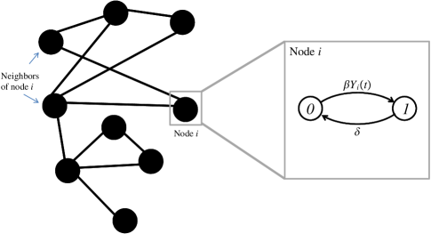
Figure 1: Schematics of a contact network along with the agent-level stochastic transition diagram for agent $i$ according to the SIS epidemic spreading model. The parameters $\beta$ and $\delta$ denote the infection rate and curing rate, respectively. $Y_{i}(t)$ is the number of the neighbors of agent $i$ that are infected at time $t$.

Denote the infection probability of the $i$-th agent by $p_{i}\triangleq\Pr[X_{i}(t)=1]$. It has been shown that the marginal probabilities $p_{i}$ do not form a closed system. Actually, the exact Markov set of differential equations has $2^{N}$ states. Van Mieghem et. al. [7] used a first order mean-field type approximation to develop the NIMFA model, a set of ordinary differential equations

$$\dot{p}_{i}=\beta(1-p_{i})\sum_{j=1}^{N}a_{ij}p_{j}-\delta p_{i},~{}i\in\{1,...,N\},$$ (1)

which represents the time evolution of the infection probability for each agent. There is no approximation on the network topology in this model. According to this model, it is proved that if the infection strength $\tau=\beta/\delta$ is less than the threshold value $\tau_{c}\triangleq\frac{1}{\lambda_{1}(A)}$, initial infection probabilities die out exponentially. If the infection strength $\tau=\beta/\delta$ is higher than $\tau_{c}$, then infection probabilities will go to non-zero steady state values.

III-B SIS Epidemic Spreading over Interconnected Networks

Consider two groups of agents of sizes $N_{1}$ and $N_{2}$. In order to facilitate the subsequent developments, we label the agents of the first graph $\mathcal{G}_{1}$ from $1$ to $N_{1}$, and the agents of the second graph $\mathcal{G}_{2}$ from $N_{1}+1$ to $N_{1}+N_{2}$. The collective adjacency matrix $A$, defined as

$$A\triangleq\begin{bmatrix}A_{11}&A_{12}\\ A_{21}&A_{22}\end{bmatrix}\in\mathbb{R}^{{}_{(N_{1}+N_{2})\times(N_{1}+N_{2})}},$$ (2)

represents the contact between all of the agents. Since the contact topology in this paper is undirected, $A_{11}$ and $A_{22}$ are symmetric matrices and $A_{21}=A_{12}^{T}$. According to definition (2), agent $i$ is connected to agent $j$ iff $(A)_{ij}=1$. A schematic of the interconnected contact network of the agents is represented in Fig. 2.

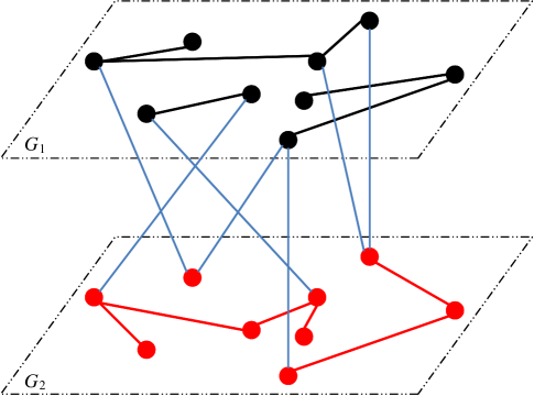
Figure 2: A schematic of the coupling between graphs $\mathcal{G}_{1}$ (in black) and $\mathcal{G}_{2}$ (in red), which each represent a contact network. The blue links represent the coupling between the nodes of the two graphs. $\mathcal{G}_{1}$ and $\mathcal{G}_{2}$ are not necessarily connected. However, the whole interconnected network is connected.

The SIS spreading model over a single graph described in Section III-A can be generalized in the following way. The curing rate for agents of graphs $\mathcal{G}_{1}$ and $\mathcal{G}_{2}$ are $\delta_{1}\in\mathbb{R}^{+}$ and $\delta_{2}\in\mathbb{R}^{+}$, respectively. The infection rates $\beta_{11},\beta_{12},\beta_{21},\beta_{22}\in\mathbb{R}^{+}$ are such that a susceptible agent of graph $\mathcal{G}_{m}$ receives the infection from an infected agent in $\mathcal{G}_{n}$ with the infection rate $\beta_{mn}$, for $m,n\in\{1,2\}$. Similar to (1), the infection probabilities of the agents evolve according to the following set of differential equations:

$$\dot{p}_{i}=(1-p_{i})\{\beta_{11}\sum_{j=1}^{N_{1}}a_{ij}p_{j}+\beta_{12}\sum_{j=N_{1}+1}^{N_{1}+N_{2}}a_{ij}p_{j}\}-\delta_{1}p_{i},\\ i\in\{1,...,N_{1}\},$$ (3)

$$\dot{p}_{i}=(1-p_{i})\{\beta_{21}\sum_{j=1}^{N_{1}}a_{ij}p_{j}+\beta_{22}\sum_{j=N_{1}+1}^{N_{1}+N_{2}}a_{ij}p_{j}\}-\delta_{2}p_{j},\\ ~{}i\in\{N_{1}+1,...,N_{1}+N_{2}\}.$$ (4)

Remark 1

Infection process is the result of interaction between a pair of agents. Therefore, actually the infection rate in (1) equals to $\beta=\mu\pi$ where $\mu\in\mathbb{R}^{+}$ is the rate that an infected agents transmits the infection and $\pi\in[0,1]$ is the probability that a susceptible agent receives a transmitted infection. Similar arguments show that the four infection rates $\beta_{11},\beta_{12},\beta_{21},\beta_{22}$ in (3) and (4) are not completely independent of each other. Having $\beta_{11}=\mu_{1}\pi_{1}$ and $\beta_{22}=\mu_{2}\pi_{2}$, the infection rates $\beta_{12}$ and $\beta_{21}$ will have a form of $\beta_{12}=\alpha\mu_{1}\pi_{2},\beta_{21}=\alpha\mu_{2}\pi_{1}$, where $\alpha\in\mathbb{R}^{+}$ is a positive scalar accounting for heterogeneity of interconnection and interaconnection. Therefore, the following constraint exists among the infection rates

$$\beta_{11}\beta_{22}=\alpha^{2}\beta_{12}\beta_{21}.$$ (5)

Comparing (1) and (3), it can be concluded that interconnection increases the probability of infection. This conclusion is actually intuitive: when interconnected with other agents, there is more possibility to receive the infection.

IV Main Results

IV-A Problem Statement

Suppose that agents of graph $\mathcal{G}_{1}$ are connected to agents of graph $\mathcal{G}_{2}$, and the overall contact among the agents is determined by $A$ defined in (2), where the following assumption holds for $\tau_{22}$.

Assumption 1

If there is no interconnection, infection cannot survive in $\mathcal{G}_{2}$, i.e.,

$$\frac{\beta_{22}}{\delta_{2}}<\frac{1}{\lambda_{1}(A_{22})}.$$ (6)

Under Assumption 1, for the infection strength $\tau_{11}=0$, the steady state value of infection probabilities of (3) and (4) are necessarily zero for each agent. In this paper, we find a threshold value $\tau_{11,c}$ such that for infection strength $\tau_{11}>\tau_{11,c}$ the steady state infection probabilities take positive values. Since interconnection always increases the chance of receiving the infection, we expect $\tau_{11,c}<1/\lambda_{1}(A_{11})$.

IV-B Equation for Epidemic Threshold

We use bifurcation theory to find the epidemic threshold. From (3) and (4), the equilibrium points of the infection probabilities satisfy the following set of algebraic equations

$$\frac{p_{i}^{\ast}}{1-p_{i}^{\ast}}=\tau_{11}\sum_{j=1}^{N_{1}}a_{ij}p_{j}^{\ast}+\tau_{12}\sum_{j=N_{1}+1}^{N_{1}+N_{2}}a_{ij}p_{j}^{\ast},\\ i\in\{1,...,N_{1}\},$$ (7)

$$\frac{p_{i}^{\ast}}{1-p_{i}^{\ast}}=\tau_{21}\sum_{j=1}^{N_{1}}a_{ij}p_{j}^{\ast}+\tau_{22}\sum_{j=N_{1}+1}^{N_{1}+N_{2}}a_{ij}p_{j}^{\ast},\\ ~{}i\in\{N_{1}+1,...,N_{1}+N_{2}\},$$ (8)

where,

$$\tau_{11}\triangleq\frac{\beta_{11}}{\delta_{1}},\tau_{12}\triangleq\frac{\beta_{12}}{\delta_{1}},\tau_{21}\triangleq\frac{\beta_{21}}{\delta_{2}},\tau_{22}\triangleq\frac{\beta_{22}}{\delta_{2}}.$$ (9)

Lemma 1

If the overall contact network is connected, the steady state values of the infection probabilities are either zero for all of the agents or absolutely positive for each agent.

Proof:

The idea of the proof is inspired from [7]. The steady state values for the infection satisfies (7) and (8). Therefore, $p_{i}^{\ast}=0$ for $\forall i\in\{1,...,N_{1}+N_{2}\}$ is a solution for the steady state infection probabilities. Suppose there exists a node $j$ such that $p_{j}^{\ast}>0$. According to (7) and (8), for any node $i$ that is a neighbor of node $j$, i.e., $a_{ij}\neq 0$, the steady state infection probability is

$$p_{i}^{\ast}=\frac{\tau_{11}\sum_{j=1}^{N_{1}}a_{ij}p_{j}^{\ast}+\tau_{12}\sum_{j=N_{1}+1}^{N_{1}+N_{2}}a_{ij}p_{j}^{\ast}}{1+\tau_{11}\sum_{j=1}^{N_{1}}a_{ij}p_{j}^{\ast}+\tau_{12}\sum_{j=N_{1}+1}^{N_{1}+N_{2}}a_{ij}p_{j}^{\ast}},$$ (10)

if $i\in\{1,...,N_{1}\}$ and

$$p_{i}^{\ast}=\frac{\tau_{21}\sum_{j=1}^{N_{1}}a_{ij}p_{j}^{\ast}+\tau_{22}\sum_{j=N_{1}+1}^{N_{1}+N_{2}}a_{ij}p_{j}^{\ast}}{1+\tau_{21}\sum_{j=1}^{N_{1}}a_{ij}p_{j}^{\ast}+\tau_{22}\sum_{j=N_{1}+1}^{N_{1}+N_{2}}a_{ij}p_{j}^{\ast}},$$

if $i\in\{N_{1}+1,...,N_{1}+N_{2}\}$, which is positive because $\sum_{j=1}^{N_{1}}a_{ij}p_{j}^{\ast}>0$ or $\sum_{j=N_{1}+1}^{N_{1}+N_{2}}a_{ij}p_{j}^{\ast}>0$. Same procedure can be applied to the neighbors of node $i$, and so on. Hence, if the contact network is connected and at least one of the agents have nonzero infection probability, then $p_{i}^{\ast}>0$ for all $i\in\{1,...,N_{1}+N_{2}\}$. ∎

Before the epidemic threshold, origin is the only solution to (7) and (8). Epidemic threshold is the critical value $\tau_{11,c}$ such that a second equilibrium point starts leaving the origin. A corollary of Lemma 1 is that the epidemic threshold $\tau_{11,c}$ is such that $p_{i}^{\ast}=0$ and $\frac{\partial p_{i}^{\ast}}{\partial\tau_{11}}>0$ for every $i\in\{1,...,N_{1}+N_{2}\}$. Taking the derivative of (7) and (8) with respect to $\tau_{11}$ at $\tau_{11}=\tau_{11,c}$ and $p_{i}^{\ast}=0$ yields

$$\frac{\partial p_{i}^{\ast}}{\partial\tau_{11}}=\tau_{11,c}\sum_{j=1}^{N_{1}}a_{ij}\frac{\partial p_{j}^{\ast}}{\partial\tau_{11}}+\tau_{12}\sum_{j=N_{1}+1}^{N_{1}+N_{2}}a_{ij}\frac{\partial p_{j}^{\ast}}{\partial\tau_{11}},\\ i\in\{1,...,N_{1}\},$$ (11)

$$\frac{\partial p_{i}^{\ast}}{\partial\tau_{11}}=\tau_{21}\sum_{j=1}^{N_{1}}a_{ij}\frac{\partial p_{j}^{\ast}}{\partial\tau_{11}}+\tau_{22}\sum_{j=N_{1}+1}^{N_{1}+N_{2}}a_{ij}\frac{\partial p_{j}^{\ast}}{\partial\tau_{11}},\\ i\in\{N_{1}+1,...,N_{1}+N_{2}\}.$$ (12)

Defining $V_{1}\triangleq[\frac{\partial p_{1}^{\ast}}{\partial\tau_{11}},...,\frac{\partial p_{N_{1}}^{\ast}}{\partial\tau_{11}}]^{T}$ and $V_{2}\triangleq[\frac{\partial p_{N_{1}+1}^{\ast}}{\partial\tau_{11}},...,\frac{\partial p_{N_{1}+N_{2}}^{\ast}}{\partial\tau_{11}}]^{T}$, the equations (11) and (12) can be equivalently expressed in the collective form as

$$\begin{bmatrix}\tau_{11,c}A_{11}&\tau_{12}A_{12}\\ \tau_{21}A_{12}^{T}&\tau_{22}A_{22}\end{bmatrix}\genfrac{[}{]}{0.0pt}{}{V_{1}}{V_{2}}=\genfrac{[}{]}{0.0pt}{}{V_{1}}{V_{2}}.$$ (13)

The critical value of the infection strengths are those for which the above equation has a positive solution. Equation (13) can be written as

$$\tau_{11,c}A_{11}V_{1}+\tau_{12}A_{12}V_{2} =V_{1},$$ (14)

$$\tau_{21}A_{12}^{T}V_{1}+\tau_{22}A_{22}V_{2} =V_{2}.$$ (15)

According to Assumption 1, if $V_{1}$ is positive then $V_{2}=\tau_{21}(I-\tau_{22}A_{22})^{-1}A_{12}^{T}V_{1}$ exists and is non-negative. Therefore, (13) is equivalently expressed as

$$HV_{1}=V_{1}$$ (16)

where $H$ is defined as

$$H\triangleq\tau_{11,c}A_{11}+\tau_{21}\tau_{12}A_{12}(I-\tau_{22}A_{22})^{-1}A_{12}^{T}.$$ (17)

IV-C Effect of Coupling on Epidemic Threshold

The rest of the analysis is to find the threshold value $\tau_{11,c}$ such that (16) has a positive solution for $V_{1}$. The following results facilitate the proof of Theorem 2, which is the main result in this paper.

Lemma 2

The number of paths of length $L$ from node $i\in\mathcal{G}_{1}$ to node $j$ corresponding to the class $(l_{1},...,l_{s})$ is:

• the $(i,j)$-th entry of $A_{11}^{l_{1}}A_{12}A_{12}^{l_{2}}A_{21}\cdots A_{21}A_{1}^{l_{s}}$, if $j\in\{1,...,N_{1}\}$,

• the $(i,j-N_{1})$-th entry of $A_{11}^{l_{1}}A_{12}A_{12}^{l_{2}}A_{21}\cdots A_{12}A_{2}^{l_{s}}$, if $j\in\{N_{1}+1,...,N_{1}+N_{2}\}$,

where $A_{11}^{0}=I_{N_{1}\times N_{1}}$ and $A_{22}^{0}=I_{N_{2}\times N_{2}}$, by convention.

Proof:

We use induction for the proof. For $L=1$, the number of paths from node $i$ to $j$ is equal to $1$ if $i$ is connected to $j$, and is zero otherwise. If $j\in\{1,...,N_{1}\}$, path of length $L=1$ corresponds to the class $(1)$. Therefore, the number of paths from node $i$ to $j$ is equal to the $(i,j)$-th entry of $A_{11}$. If $j\in\{N_{1}+1,...,N_{1}+N_{2}\}$, then a path of length $L=1$ corresponds to the class either $(0,0)$. In this case, the number of paths from node $i$ to $j$ is equal to the $(i,j-N_{1})$-th entry of $A_{12}=A_{1}^{0}A_{12}A_{2}^{0}$. Therefore for $L=1$, the Lemma is correct.

Assume that for $L=L_{0}$ the lemma statement is correct. Consider the first case where $j\in\{1,...,N_{1}\}$. A path of length $L=L_{0}+1$ from $i$ to $j$ is either of the class $(l_{1},...,l_{s}+1)$ or $(l_{1},...,l_{s},0)$. Such a path can be constructed from paths of length $L_{0}$ from $i$ to $k$ of the class $(l_{1},...,l_{s})$ then connected to node $j$ from node $k$.

If the path from $i$ to $j$ is of class $(l_{1},...,l_{s}+1)$, then the number of such paths is

$$\sum_{k=1}^{N_{1}}(A_{11}^{l_{1}}A_{12}A_{12}^{l_{2}}A_{21}\cdots A_{21}A_{1}^{l_{s}})_{ik}(A_{1})_{kj}=\\ A_{11}^{l_{1}}A_{12}A_{12}^{l_{2}}A_{21}\cdots A_{21}A_{1}^{l_{s}+1}.$$

If the path from $i$ to $j$ is of class $(l_{1},...,l_{s},0)$, then the number of such paths is

$$\sum_{k=N_{1}+1}^{N_{1}+N_{2}}(A_{11}^{l_{1}}A_{12}A_{12}^{l_{2}}A_{21}\cdots A_{21}A_{1}^{l_{s}})_{i(k-N_{1})}(A_{12})_{(k-N_{1})j}\\ =A_{11}^{l_{1}}A_{12}A_{12}^{l_{2}}A_{21}\cdots A_{21}A_{1}^{l_{s}}A_{12}\\ =A_{11}^{l_{1}}A_{12}A_{12}^{l_{2}}A_{21}\cdots A_{21}A_{1}^{l_{s}}A_{12}A_{2}^{0}.$$

Hence, the theorem statement is correct for $L=L_{0}+1$ and $j\in\{1,...,N_{1}\}$. Similar procedure can be followed to conclude the same result for $j\in\{N_{1}+1,...,N_{1}+N_{2}\}$. ∎

Theorem 1

The matrix $H_{T}$ defined as

$$H_{T}\triangleq A_{11}+\alpha^{2}\tau_{22}A_{12}(I-\tau_{22}A_{22})^{-1}A_{12}^{T}.$$ (18)

is irreducible if the coupled network is connected.

Proof:

We show that

$$\bar{H}_{T}\triangleq A_{11}+A_{12}A_{12}^{T}+\sum_{k=1}^{N_{2}-1}A_{12}A_{22}^{k}A_{12}^{T}$$ (19)

is irreducible. If $\bar{H}_{T}$ is shown to be irreducible, then $A_{11}+\alpha^{2}\tau_{22}A_{12}A_{12}^{T}+\alpha^{2}\tau_{22}\sum_{k=1}^{N_{2}-1}\tau_{22}^{k}A_{12}A_{2}^{k}A_{12}^{T}$ is irreducible. And hence, $H_{T}=A_{11}+\alpha^{2}\tau_{22}A_{12}A_{12}^{T}+\alpha^{2}\tau_{22}\sum_{k=1}^{\infty}\tau_{22}^{k}A_{12}A_{2}^{k}A_{12}^{T}=A_{11}+\alpha^{2}\tau_{22}A_{12}(I-\tau_{22}A_{22})^{-1}A_{12}^{T}$ is irreducible and the proof is completed.

If $\mathcal{G}_{1}$ is a connected graph, then $A_{11}$ and as consequence $\bar{H}_{T}$ is irreducible. Assume that $A_{11}$ does not represent a connected graph. Therefore, there exists a pair $i$, $j$ such that there is no path between them in $\mathcal{G}_{1}$. However, since the whole interconnected network is connected, there exists a path from $i$ to $j$. Suppose, the path is of class $(l_{1,1},l_{2,1},l_{1,2},l_{2,2},....,l_{2,s},l_{1,s+1})$, i.e., it makes $l_{1,1}$ jumps in $\mathcal{G}_{1}$ to reach vertex $k_{1}^{out}$, then it leaves $\mathcal{G}_{1}$ and enters $\mathcal{G}_{2}$ and makes $l_{2,1}$ jumps in $\mathcal{G}_{2}$, then enters $\mathcal{G}_{1}$ at vertex $k_{1}^{in}$. This process goes on until it makes $l_{1,s+1}$ jumps in $\mathcal{G}_{1}$ from $k_{s}^{in}$ to reach vertex $j$. Matrix $\bar{H}_{T}$ is proved to be irreducible if we show that $(k_{u}^{out},k_{u}^{in})$-th entry of $\bar{H}_{T}$ is positive for $u=1,...,s$. Since, there is path from $k_{u}^{out}$ to $k_{u}^{in}$ which is of the class $(0,l_{2,u},0)$, the $(k_{u}^{out},k_{u}^{in})$-th entry of $A_{12}A_{22}^{l_{2,u}}A_{12}^{T}\geq 1$,because it is the number of such paths according to Lemma 2. As a consequence, $(k_{u}^{out},k_{u}^{in})$-th entry of $\bar{H}_{T}$ is positive and therefore $\bar{H}_{T}$ is irreducible. Hence, the proof is completed. ∎

Theorem 2

For

$$\tau_{11,c}=\dfrac{1}{\lambda_{1}(H_{T})},$$ (20)

where $H_{T}$ is defined in (18), the equation (13) has positive solution for $V_{1}$ and $V_{2}$. That is $\tau_{11,c}$ is the epidemic threshold.

Proof:

According to (5) and the definitions (9), we have

$$\tau_{21}\tau_{12}=\alpha^{2}\tau_{11,c}\tau_{22}\text{.}$$ (21)

Substituting for $\tau_{21}\tau_{12}$ in (17), equation (16) gets the form

$$\tau_{11,c}H_{T}V_{1}=V_{1},$$ (22)

where $H_{T}$ is defined in (18). In order for (22) to have solutions, $\tau_{11,c}$ must be the inverse of one of the eigenvalues of $H_{T}$. However, the corresponding eigenvector $V_{1}$ must have all positive entries. According to Theorem 1, $H_{T}$ is an irreducible matrix. Therefore, $V_{1}$ is positive only for the eigenvector corresponding to the largest eigenvalue. Therefore, $\tau_{11,c}$ is equal to $1/\lambda_{1}(H_{T})$. ∎

IV-D Interconnection Topology and Epidemic Spreading Modes

We used a bifurcation method to find an expression for the epidemic threshold. According to our definition, the epidemic threshold is a critical value such that for any infection strength $\tau_{11}>\tau_{11,c}$, the steady state values of the infection probabilities are positive. Consider the special case where the infection strength $\tau_{22}$ is very close to the spectral radius $\lambda_{1}(A_{22})$, i.e., $\tau_{22}\rightarrow\lambda_{1}(A_{22})$. According to (18) and (20), the epidemic threshold $\tau_{11,c}\rightarrow 0$ as far as the whole contact network is connected. This argument is true even for very weak interconnection between the two networks $\mathcal{G}_{1}$ and $\mathcal{G}_{2}$. The reason for this observation is that since $\tau_{22}\rightarrow\lambda_{1}(A_{22})$, only a small amount of interconnection will lead to an outbreak in $\mathcal{G}_{2}$. Since, the probability of infection in $\mathcal{G}_{2}$ becomes a positive value, according to Lemma 1, the probability of infection in $\mathcal{G}_{1}$ is also positive. Therefore in the case of $\tau_{22}\rightarrow\lambda_{1}(A_{22})$ and weak interconnection, the positive infection probabilities in $\mathcal{G}_{1}$ for small values of $\tau_{11}$ is only due to epidemic outbreak in $\mathcal{G}_{2}$.

The numerical simulations in Section V illustrates three possible curves of $\tau_{11,c}$ as a function of $\tau_{22}$, as shown in Fig. 3. Here, the blue curve belongs to the case of weak interconnection between the two graphs. As can be seen, the decrease in the epidemic threshold $\tau_{11,c}$ is very slow for small values of $\tau_{22}$, while there is a quite sharp drop in the values of $\tau_{11,c}$ as $\tau_{22}\rightarrow\lambda_{1}(A_{22})$. For strong interconnection topology, shown by the green curve, the value of $\tau_{11,c}$ is decreasing quickly for small values of $\tau_{22}$. In this case, the infection in $\mathcal{G}_{1}$ starts to grow not only as the result of receiving the infection from $\mathcal{G}_{2}$, but also as the result of a survivable internal infection force. The red curve is an intermediate between the two spreading modes.

Theorem 3

The derivative $\frac{d\tau_{11,c}}{d\tau_{22}}$ at $\tau_{22}=0$ is

$$\left.\frac{d\tau_{11,c}}{d\tau_{22}}\right|_{\tau_{22}=0}=\frac{\alpha^{2}\left\|A_{12}^{T}x_{1}\right\|_{2}^{2}}{\lambda_{1}^{2}(A_{11})},$$ (23)

where $x_{1}$ is the eigenvector of $A_{11}$ belonging to $\lambda_{1}(A_{11}).$

Proof:

The matrix $H_{T}$ from (18) can be written as

$$H_{T}\triangleq A_{11}+\alpha^{2}\tau_{22}A_{12}A_{12}^{T}+o(\tau_{22})\text{.}$$

Therefore, taking the derivative of (22) with respect to $\tau_{22}$ at $\tau_{22}=0$ yields

$$\frac{d\tau_{11,c}}{d\tau_{22}}A_{11}x_{1}+\frac{1}{\lambda_{1}(A_{11})}(\alpha^{2}A_{12}A_{12}^{T})x_{1}\\ +(\frac{1}{\lambda_{1}(A_{11})}A_{11}-I)\frac{dV_{1}}{d\tau_{22}}=0.$$ (24)

Multiplying (24) by $x_{1}^{T}$ from left, we get

$$\frac{d\tau_{11,c}}{d\tau_{22}}x_{1}^{T}A_{11}x_{1}+\frac{\alpha^{2}}{\lambda_{1}(A_{11})}x_{1}^{T}(A_{12}A_{12}^{T})x_{1}\\ +x_{1}^{T}(\frac{1}{\lambda_{1}(A_{11})}A_{11}-I)\frac{dV_{1}}{d\tau_{22}}=0.$$ (25)

In (25), since $x_{1}$is the normalized eigenvector of $A_{11}$ corresponding to $\lambda_{1}(A_{11})$, we have $x_{1}^{T}A_{11}x_{1}=\lambda_{1}(A_{11})$ and $x_{1}^{T}(\frac{1}{\lambda_{1}(A_{11})}A_{11}-I)=0$ for $A_{11}$ is symmetric. Therefore, equation (25) becomes

$$\lambda_{1}(A_{11})\frac{d\tau_{11,c}}{d\tau_{22}}+\frac{\alpha^{2}}{\lambda_{1}(A_{11})}(A_{12}^{T}x_{1})^{T}(A_{12}^{T}x_{1})=0.$$ (26)

Hence, $\frac{d\tau_{11,c}}{d\tau_{22}}$ is found to be (23). ∎

According to (23) and the proceeding arguments, we define interconnection topology measure

$$\Omega\left(\mathcal{G}_{1},\mathcal{G}_{2}\right)\triangleq\frac{\alpha^{2}\left\|A_{12}^{T}x_{1}\right\|_{2}^{2}}{\lambda_{1}(A_{11})\lambda_{1}(A_{22})}.$$ (27)

If $\Omega\left(\mathcal{G}_{1},\mathcal{G}_{2}\right)<1$, then for the infection strength $\tau_{11}$ right above the threshold $\tau_{11,c}$ in (20), the positive infection probability in $\mathcal{G}_{1}$ is mostly due to external infections from $\mathcal{G}_{2}$. While if $\Omega\left(\mathcal{G}_{1},\mathcal{G}_{2}\right)>1$, then for the infection strength $\tau_{11}$ right above the threshold $\tau_{11,c}$ in (20), the positive infection probability in $\mathcal{G}_{1}$ is mostly due to a survivable internal infection force as the result of increased effective level of contact among agents of $\mathcal{G}_{1}$.

Remark 2

A very interesting property of $\Omega\left(\mathcal{G}_{1},\mathcal{G}_{2}\right)$ defined in (27) is that it is a purely topological measure and does not depend on the epidemic parameters.

V Numerical Simulation Results

We have generated two graphs according to the small world random network model [19]. The first network has $N_{1}=500$ vertices with Watts and Strogatz parameters for mean degree $K_{1}=10$ and the rewiring probability $\beta_{1}=0.2$. For this graph, the spectral radius is found to be $\lambda_{1}(A_{11})=22.0586$. The second network has $N_{2}=100$ vertices with the Watts and Strogatz parameters for mean degree $K=2$ and the rewiring probability $\beta_{2}=0.1$. For this graph, the spectral radius is found to be $\lambda_{1}(A_{22})=4.3$. For the interconnection of these two graphs, we use the following rule. All the potential edges between the first graph and the second graph are active with some probability $\omega$, to be chosen.

In the first simulation, $\bar{\tau}_{c1}=\lambda_{1}(A_{11})\tau_{11,c}$ is plotted as a function of $\bar{\tau}_{2}=\lambda_{1}(A_{22})\tau_{22}$, for three different values of $\omega=0.01,0.042,0.2$. The numerical results for the three cases are shown in Fig. 3.

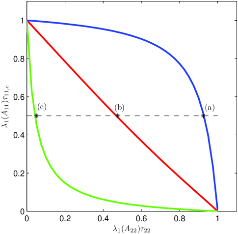
Figure 3: Normalized epidemic threshold $\bar{\tau}_{c1}=\lambda_{1}(A_{11})\tau_{11,c}$ of graph $\mathcal{G}_{1}$ as a function of the normalized infection strength $\bar{\tau}_{2}=\lambda_{1}(A_{22})\tau_{22}$ of graph $\mathcal{G}_{2}$. The interconnection in (a) $\omega=0.01$, the blue curve, (b) $\omega=0.042$, red curve, and (c) $\omega=0.2,$ green curve. A $\%50$ reduction of the epidmeic threshold is observed for the normalized infection strengths (a) $\bar{\tau}_{2}=0.925$, (b) $\bar{\tau}_{2}=0.5$, (c) $\bar{\tau}_{2}=0.05$.

As can be seen from the blue curve, which is for $\omega=0.01$, for weak interconnection among the graphs the emergence of positive steady state values for the infection probability in graph $\mathcal{G}_{1}$ is due to an outbreak in $\mathcal{G}_{2}$. While for strong interconnection $\omega=0.2$, which is shown with the green curve in Fig. 3, the emergence of positive steady state values for the infection probability in graph $\mathcal{G}_{1}$ is more due to increased level of effective contact among the agents in $\mathcal{G}_{1}$. The red curve in Fig. 3 belongs to an intermediate interconnection strength, here $\omega=0.042$.

According to Fig. 3,a $\%50$ reduction of the epidemic threshold is observed in $\mathcal{G}_{1}$for (a) $\omega=0.01$ and $\bar{\tau}_{2}=0.925$, (b) $\omega=0.042$ and $\bar{\tau}_{2}=0.5$, (c) $\omega=0.2$ and $\bar{\tau}_{2}=0.05$. We have plotted the curves of $\bar{p}_{1}^{\ast}=\frac{1}{N_{1}}\sum_{i=1}^{N_{1}}p_{i}^{\ast}$ as a function of $\tau_{11}\lambda_{1}(A_{11})$. We have found the equilibrium values of $p_{i}^{\ast}$ by solving the algebraic equations (7) and (8). The numerical method for solving these equations is presented in the Appendix.

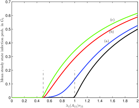
Figure 4: The mean steady state infection probability in $G_{1}$ as a function of the normalized infection strength of $\lambda_{1}(A_{11})\tau_{11}$ for graph $G_{1}$. Black curve corresponds to the case where there is no interconnection. In this case, the epidemic threshold is $\tau_{11,c}=1/\lambda_{1}(A_{11})$. All the other curves correspond to the case where $\tau_{11,c}=\frac{1}{2}\times 1/\lambda_{1}(A_{11})$. For (a) the blue curve $\omega=0.01$ and $\bar{\tau}_{2}=0.925$, (b) the red curve $\omega=0.042$ and $\bar{\tau}_{2}=0.5$, (c) the green curve $\omega=0.2$ and $\bar{\tau}_{2}=0.05$.

VI Conclusion

In epidemic modeling, the term infection strength indicates the ratio of infection rate and cure rate. If the infection strength is higher than a certain threshold then the epidemic spreads through the population and persists in the long run. For a single generic graph representing the contact network of the population under consideration, the epidemic threshold turns out to be equal to the inverse of the spectral radius of the contact graph. However, in a real world scenario it is not possible to isolate a population completely: there is always some interconnection with another network, which partially overlaps with the contact network. We study the spreading process of a susceptible-infected-susceptible (SIS) type epidemic model in an interconnected network of two general graphs. First, we prove that interconnection always increases the probability of infection. Second, we find that the epidemic threshold for a network interconnected to another network with a given infection strengths rigorously derived as the spectral radius of a new matrix which accounts for the two networks and their interconnection links. The main contribution of this paper is the use of spectral analysis to analyze epidemic spreading in interconnected networks. Our results have implications for the broad field of epidemic modeling and control.

VII Acknowledgement

This work was supported by the National Agricultural Biosecurity Center (NABC) at Kansas State University. It was also based on work partially supported by the US National Science Foundation, while one of the authors, Fahmida N. Chowdhury, was working at the Foundation. Any opinion, finding, and conclusions or recommendations expressed in this material are those of the authors and do not necessarily reflect the views of the National Science Foundation.

VIII Appendix

In order to numerically solve (7) and (8), we can use the recursive formula

$$y_{i}(k+1)=\tau_{11}\sum_{j=1}^{N_{1}}a_{ij}\frac{y_{j}(k)}{1+y_{j}(k)}+\tau_{12}\sum_{j=N_{1}+1}^{N_{1}+N_{2}}a_{ij}\frac{y_{j}(k)}{1+y_{j}(k)},\\ i\in\{1,...,N_{1}\},$$ (28)

$$y_{i}(k+1)=\tau_{21}\sum_{j=1}^{N_{1}}a_{ij}\frac{y_{j}(k)}{1+y_{j}(k)}+\tau_{22}\sum_{j=N_{1}+1}^{N_{1}+N_{2}}a_{ij}\frac{y_{j}(k)}{1+y_{j}(k)},\\ i\in\{N_{1}+1,...,N_{1}+N_{2}\},$$ (29)

which converges to the fixed points $y_{i}^{\ast}:=\frac{p_{i}^{\ast}}{1-p_{i}^{\ast}}$, for $i\in\{1,...,N_{1}+N_{2}\}$. The steady state values of the infection probabilities are then $p_{i}^{\ast}=\frac{y_{i}^{\ast}}{1+y_{i}^{\ast}}$.

References

• [1] J. Shao, S. Buldyrev, S. Havlin, and H. Stanley, “Cascade of failures in coupled network systems with multiple support-dependence relations,” Physical Review E, vol. 83, no. 3, p. 036116, 2011.
• [2] C. D. Brummitt, R. M. D’Souza, and E. A. Leicht, “Suppressing cascades of load in interdependent networks,” Proceedings of the National Academy of Sciences, 2012.
• [3] S. Funk and V. Jansen, “Interacting epidemics on overlay networks,” Physical Review E, vol. 81, no. 3, p. 036118, 2010.
• [4] M. Dickison, S. Havlin, and H. Stanley, “Epidemics on interconnected networks,” Physical Review E, vol. 85, no. 6, p. 066109, 2012.
• [5] A. Saumell-Mendiola, M. A. Serrano, and M. Boguñá, “Epidemic spreading on interconnected networks,” Phys. Rev. E, vol. 86, p. 026106, Aug 2012.
• [6] Y. Wang and G. Xiao, “Effects of interconnections on epidemics in network of networks,” in Wireless Communications, Networking and Mobile Computing (WiCOM), 2011 7th International Conference on, sept. 2011, pp. 1–4.
• [7] P. Van Mieghem, J. Omic, and R. Kooij, “Virus spread in networks,” IEEE/ACM Transactions on Networking, vol. 17, no. 1, pp. 1–14, 2009.
• [8] R. Pastor-Satorras and A. Vespignani, “Epidemic dynamics and endemic states in complex networks,” Phys. Rev. E, vol. 63, no. 6, p. 066117, May 2001.
• [9] A. V. Goltsev, S. N. Dorogovtsev, J. G. Oliveira, and J. F. F. Mendes, “Localization and spreading of diseases in complex networks,” Phys. Rev. Lett., vol. 109, p. 128702, Sep 2012.
• [10] F. Sahneh and C. Scoglio, “Epidemic spread in human networks,” in Proceedings of IEEE Conference on Decision and Control, 2011.
• [11] ——, “Optimal information dissemination in epidemic networks,” in Proceedings of IEEE Conference on Decision and Control, 2012, to appear.
• [12] M. Youssef and C. Scoglio, “An individual-based approach to SIR epidemics in contact networks,” Journal of Theoretical Biology, vol. 283, no. 1, pp. 136–144, 2011.
• [13] S. C. Ferreira, C. Castellano, and R. Pastor-Satorras, “Epidemic thresholds of the susceptible-infected-susceptible model on networks: A comparison of numerical and theoretical results,” arXiv:1206.6728v1, 2012.
• [14] V. Preciado and A. Jadbabaie, “Moment-based analysis of spreading processes from network structural information,” arXiv:1011.4324, 2010.
• [15] N. Bailey, The mathematical theory of infectious diseases and its applications.   London, 1975.
• [16] Y. Moreno, R. Pastor-Satorras, and A. Vespignani, “Epidemic outbreaks in complex heterogeneous networks,” The European Physical Journal B - Condensed Matter and Complex Systems, vol. 26, pp. 521–529, 2002.
• [17] R. Diestel, “Graph theory, volume 173 of graduate texts in mathematics,” Springer, Heidelberg, vol. 91, p. 92, 2005.
• [18] P. Van Mieghem, Graph Spectra for Complex Networks.   Cambridge Univ Pr, 2011.
• [19] M. Newman, D. Watts, and S. Strogatz, “Random graph models of social networks,” Proceedings of the National Academy of Sciences of the United States of America, vol. 99, no. Suppl 1, pp. 2566–2572, 2002.