Distant galaxy clusters in the XMM Large Scale Structure survey

Abstract

Distant galaxy clusters provide important tests of the growth of large scale structure in addition to highlighting the process of galaxy evolution in a consistently defined environment at large look back time. We present a sample of 22 distant ($z>0.8$) galaxy clusters and cluster candidates selected from the 9 deg² footprint of the overlapping X-ray Multi Mirror (XMM) Large Scale Structure (LSS), CFHTLS Wide and Spitzer SWIRE surveys. Clusters are selected as extended X-ray sources with an accompanying overdensity of galaxies displaying optical to mid-infrared photometry consistent with $z>0.8$. Nine clusters have confirmed spectroscopic redshifts in the interval $0.8<z<1.2$, four of which are presented here for the first time. A further 11 candidate clusters have between 8 and 10 band photometric redshifts in the interval $0.8<z<2.2$, while the remaining two candidates do not have information in sufficient wavebands to generate a reliable photometric redshift. All of the candidate clusters reported in this paper are presented for the first time. Those confirmed and candidate clusters with available near infrared photometry display evidence for a red sequence galaxy population, determined either individually or via a stacking analysis, whose colour is consistent with the expectation of an old, coeval stellar population observed at the cluster redshift. We further note that the sample displays a large range of red fraction values indicating that the clusters may be at different stages of red sequence assembly. We compare the observed X-ray emission to the flux expected from a suite of model clusters and find that the sample displays an effective mass limit $M_{200}\sim 1\times 10^{14}\rm M_{\odot}$ with all clusters displaying masses consistent with $M_{200}<5\times 10^{14}\rm M_{\odot}$. This XMM distant cluster study represents a complete sample of X-ray selected $z>0.8$ clusters. We discuss the importance of this sample to investigate the abundance of high redshift clusters and to provide a relatively unbiased view of distant cluster galaxy populations.

1 Introduction

Observations of galaxy clusters provide crucial insight into the development of structure in the Universe, from the growth of clusters themselves, to the evolution of their member galaxies. Furthermore, cluster studies yield important constraints on cosmological models through tests of the growth of structure (e.g. Vikhlinin et al. 2009; Pierre et al. 2011). The greatest constraining power on cosmological parameters and on the co-evolution of galaxies and clusters requires large, well-controlled samples of clusters out to $z>1$. To date, a number of techniques have been successfully applied in order to generate such samples of clusters at $z<1$. These include approaches based upon detecting galaxy overdensities (in a combination of apparent colour and sky position; e.g. Postman et al. 1996; Gladders & Yee 2005), extended X-ray sources (e.g. Gioia et al. 1990; Böhringer et al. 2000; Burenin et al. 2007; Mehrtens et al. 2012) and the Sunyaev-Zel’dovich decrement observed toward the Cosmic Microwave Background (e.g. Menanteau et al. 2010; Reichardt et al. 2012).

Although the systematic estimation of the cluster number density above $z>1$ is an important issue the search for high redshift clusters is made difficult by the faintness of the cluster signal, e.g. small galaxy over-density in optical and near-infrared (NIR) imaging, weak X-ray emission whose extent is difficult to assess, etc. However, should X-ray imaging observations of sufficient depth and spatial resolution be executed, the detection of high redshift clusters via spatially-extended emission is advantageous as it provides clear evidence of hot gas confined within a gravitational potential well. Care must be taken though to assess the extent to which faint X-ray active galactic nuclei (AGN) may mimic or modify the significance and spatial extent of cluster emission and its spectral form (e.g. Branchesi et al. 2007; Pierre et al. 2012).

Systematic searches for high redshift galaxy clusters in X-rays are currently being conducted via dedicated XMM surveys (XDCP Fassbender et al. 2011; XMM-LSS Pierre et al. 2007; Bremer et al. 2006; Andreon et al. 2005, this work; XCS Romer et al. 2001; Stanford et al. 2006). These surveys employ quantitative algorithms to identify extended sources and are characterised by accurate selection functions and a clearly defined relationship between cluster observables (such as X-ray luminosity) and total cluster mass (Reichert et al., 2011). Galaxy clusters at $z>1$ may also be detected by the extension of successful “red sequence” searches to near– and mid–infrared (MIR) wavebands in order to detected the redshifted emission from distant galaxies (e.g. Muzzin et al. 2009). An associated technique employed by the IRAC Shallow Cluster Survey (Eisenhardt et al., 2008) identifes clusters to $z<1.5$ as stellar mass overdensities in multi-band photometric redshift slices. Each MIR imaging technique has proven very successful at identifying large numbers of candidate and confirmed clusters.

Galaxy clusters at $z<1$ have been employed extensively to study their member galaxy populations and indicate that they are composed of uniformly old stellar populations where the bulk of their stars formed at $z=3$ or greater (Jaffé et al., 2011). In addition, low redshift clusters display strong population trends such as the morphology–density relation (e.g. Dressler et al. 1997). Such relations reflect the dominance of bright, red, bulge-dominated galaxies in cluster cores. Observing clusters at high redshift provides an opportunity to approach the epoch when the progenitors of low-redshift galaxies where assembled. Indeed impressive direct evidence is emerging of both red sequence truncation (Rudnick et al., 2012) and merger driven galaxy assembly (Lotz et al., 2012) in a MIR selected (yet X-ray detected) cluster at $z=1.6$. The evolution of the brightest cluster galaxies (BCGs) in distant clusters presents a more complex picture: Lidman et al. (2012) report that the stellar mass of BCGs in 160 clusters spanning $0.03<z<1.63$ grow steadily with decreasing redshift in a manner consistent with a semi-analytic model. In potential contrast to such evolution in high redshift cluster galaxies, Stott et al. (2010) report that the stellar mass contained in the BCGs of a sample of 20, $0.8<z<1.5$ clusters has changed little between the epoch of observation and the present day. Such trends observed in heterogeneously assembled samples will be better understood by performing similarly extensive analyses upon a complete sample of high redshift clusters selected employing a single method (e.g. Fassbender et al. 2011).

The XMM-LSS survey is well placed to contribute to this investigation: covering 11 deg² with X-ray imaging to a depth of $\sim 1\times 10^{-14}$ erg s^-1 cm^-2 for extended sources in the [0.5-2]keV waveband and accompanied by optical and MIR photometry. The XMM-LSS project has previously demonstrated the ability to identify clusters to $z=1.2$ (Bremer et al. 2006) and has published $z<1$ cluster number counts selected according to a clear, quantitative selection function (Pacaud et al. 2007).

This paper presents the XMM-LSS distant cluster sample. These are defined to be extended X-ray sources at $z>0.8$ and consist of spectroscopically confirmed clusters together with a number of candidate clusters supported by a detailed photometric redshift analysis. The distant cluster sample has been identified from the full sample of extended X-ray sources within a 9 deg²  sub-area of the XMM-LSS survey and in this sense it represents a complete sample of X-ray selected distant clusters. In particular, the methods employed to determine whether a given extended X-ray source is or is not a distant cluster are selected to minimise any potential bias such as the presence of a strong red sequence. In this sense the sample should be as complete as possible and should provide an unbiased perspective of the galaxy populations in distant X-ray clusters.

The structure of the paper is as follows. Section 2 describes the construction of the distant cluster sample (containing both spectroscopically confirmed and candidate systems) and the multi-wavelength data sets used to define it in addition to presenting images of the sources in the sample. Section 3 describes the approaches taken to explore which of the candidate systems have clear photometric evidence for being genuine distant clusters. Section 4 discusses the results of applying these approaches and explores the diversity of properties shown by the likely high redshift systems.

This paper employs a Friedmann-Robertson-Walker cosmological model described by the parameters $\Omega_{M}=0.3$, $\Omega_{\Lambda}=0.7$, $H_{0}=70\rm\,kms^{-1}Mpc^{-1}$. An angular scale of 1′ corresponds to a transverse physical scale of 480 kpc, 508 kpc and 502 kpc at redshifts $z=1$, 1.5 and 2 respectively. All photometry is quoted in the AB system.

2 The XMM-LSS survey sample

The XMM-LSS survey currently covers approximately 11 deg² and is described in Chiappetti et al. (2012) and Clerc et al. (2013). Galaxy clusters are detected as extended X-ray sources and are classified as either C1 or C2 on the basis of their surface brightness characteristics (Pacaud et al., 2006). The effective flux limit is $\sim 1\times 10^{-14}$erg s^-1 cm^-2 for extended sources.

Visual inspection of the X-ray images of individual systems along with their optical and NIR images confirm that the C1 class represents an uncontaminated sample of extended X-ray sources (mainly clusters but with some detections of X-ray halos in very low redshift galaxies, Pacaud et al. 2006). The C2 class displays a contamination rate of 30-50%, with the main sources of contamination being misclassified point sources and artefacts on the X-ray image. These contaminants are typically removed by visual inspection of the X-ray image prior to further analysis.

The 11 deg² XMM-LSS sample contains 50 C1 and 60 C2 sources, of which 44 C1 and 27 C2 sources have confirmed redshifts from optical spectroscopy. The redshift distribution of confirmed sources ranges over $0.05<z<1.22$. The lower spectroscopic confirmation rate for the C2 sources arises due to a) the lower priority placed on follow-up of such sources compared to C1 sources and b) the increased difficulty of following up fainter, lower quality detections.

The analysis used to generate the XMM-LSS distant cluster sample is based upon a 9 deg² subregion of the XMM-LSS field. This region represents the common footprints of the XMM-LSS, Canada France Hawaii Telescope Legacy Survey (CFHTLS) W1 and Spitzer SWIRE 3.6 and 4.5$\micron$ surveys and contains 88 C1$+$C2 sources (of which 55 have spectroscopic redshifts). NIR imaging drawn from a variety of sources (i.e. the UKIDSS and WIRDS surveys in addition to individual CFHT/WIRCam and VLT/HAWKI images) exists for many of the spectroscopically confirmed and candidate distant systems, with the available bands and depth varying on a source-by source basis. The principal data sets and their processing are described below.

2.1 X-ray photometry

The characterisation and measurement of extended sources in the XMM-LSS survey is described in detail in Pacaud et al. (2006) and Adami et al. (2011) and we summarise the important features of the analysis here. Sources are detected above a specified pixel threshold by appliying the SExtractor routine to a multi-scale wavelet reconstruction of the XMM science image. Individual sources are characterised as either extended or point-like on the basis of the likelihood values of appropriate models applied to each source. Taking the example of an extended source, nearby point-sources identified individually by the detection algorithm are masked when performing the source extended fit using the SExtractor segmentation map (Pacaud et al., 2006). Therefore the extent likelihood used for C1/C2 classification is almost free from contamination by bright point sources. Faint point-sources contaminating the extended source emission and not deblended by the algorithm may be present, particularly in regions close to the cluster centre. Accounting for them is challenging given the faintness of our objects and their compactness relative to XMM point spread function.

We compute X-ray fluxes for the extended sources associated with spectroscopically confirmed and candidate clusters in the [0.5-2] keV band employing the procedure outlined in Adami et al. (2011). The method applies a curve-of-growth analysis to the X-ray count rate data which confers the advantage of being free of any profile assumptions applied to the extended X-ray source. We estimate that the application of a finite size aperture used for these measurements recovers 80-90% of the total count rate of the cluster and we note that this bias is lower than the statistical error of our measurements. The flux measurement step allows a further check for additional blended emission. Point sources lying close to but off the cluster central region are either identified by the detection algorithm or flagged visually. In both cases their contribution to the total flux is excluded from the extraction region, and the missing area is accounted for by assuming a circularly symmetric flux profile. The fluxes were obtained assuming a fixed conversion factor of $9\times 10^{−13}\rm(ergs^{-1}cm^{-2})/(cnts~{}s^{-1})$. This value was calculated using Xspec from an APEC emission model with the following parameters: $z=1$, $T=4$ keV, $N_{H}=2.6\times 10^{20}\rm cm^{−2}$, $Ab=0.3$ (note that the conversion factor changes by less than 5% for $z=1.5$ and $T=4$ keV). Bolometric luminosities were calculated with Xspec employing the measured fluxes, the cluster redshift (quoted in Table 1) and the fitted cluster temperature (Bremer et al. 2006; Pacaud et al. 2007) or assuming $T=4$ keV if no temperature was available. Flux and luminosity values for each cluster are listed in Table 1.

2.2 Multi-wavelength photometric data

As noted above, most of the data used in this analysis are taken from existing large area surveys which cover part or all of the XMM-LSS region. Descriptions of the CFHTLS and Spitzer SWIRE data used in the paper are described in Gwyn (2012) and Chiappetti et al. (2012) respectively. Large area NIR survey data provided $J$, $H$ and/or $K$-band imaging for a number of the C1 and C2 $z>0.8$ candidates. These data came from either the UKIDSS Deep Extragalactic Survey (DXS DR8; see Lawrence et al., 2007) or the WIRCam Deep Survey (WIRDS; Bielby et al., 2010). Typical depths ($5\sigma$) for these data are $J=23.4,K=22.9$ (DXS) and $J=24.7,H=24.7,Ks=24.7$ (WIRDS). NIR imaging data for the remaining sources in the distant cluster sample were obtained with principal investigator programs using VLT/HAWKI and CFHT/WIRCam and are described below. Details of the available multi-wavelength photometry for each $z>0.8$ system, both candidate and confirmed, are given in Table 1.

Table 1: Distant clusters in the XMM-LSS survey. These sources represent all C1$+$C2 sources (Section 2) within the approximately 9 deg² XMM-LSS/CHFTLS/SWIRE footprint that cannot be unambiguously associated with a $z<0.8$ cluster or galaxy. Spectroscopically confirmed distant clusters are displayed in the upper section of the table and have their redshift values indicated. Each is also described by an official XLSSC identifier. Candidate distant clusters are displayed in the middle section of the table and their photometric redshift values (where computed) are indicated with accompanying uncertainty. Unknown sources are displayed in the lower section of the table and do not have a redshift value. Each cluster is further identified using a sequential number (column 1) to simplify their discussion in this paper. In subseqent publications that refer to these sources, we recommend using either the cluster names or the XLSSC numbers which are the only IAU validated labelings. The procedures used to compute the X-ray flux and luminosity measures are described in Section 2.1.

Number	Cluster name	XLSSC	Class	R.A.	Dec.	redshift	Flux [0.5-2]keV	$L_{X},bol$	wavebands	Reference for
				(J2000)	(J2000)		$\times 10^{-14}$erg s-1 cm-2	$\times 10^{44}$erg s-1		spectroscopic redshift
01	XLSS    J022400.4-032529	032	C2	36.002	-3.424	0.803	$1.56\pm 0.43$	$1.16\pm 0.32$	$grz3.6\micron 4.5\micron$	Section 2.4
02	XLSS    J022233.8-045803	066	C2	35.641	-4.968	0.833	$1.13\pm 0.27$	$0.92\pm 0.22$	$ugrizK3.6\micron 4.5\micron$	Section 2.4
03	XLSSU J021832.0-050105	064	C2	34.633	-5.106	0.875	$1.48\pm 0.12$	$1.36\pm 0.11$	$ugriz3.6\micron 4.5\micron$	Adami et al. (2011)
04	XLSSU J021524.1-034332	067	C1	33.850	-3.726	1.003	$6.26\pm 0.64$	$7.85\pm 0.80$	$ugrizYJK_{s}3.6\micron 4.5\micron$	Section 2.4
05	XLSS    J022253.6-032828	048	C1	33.850	-3.726	1.005	$1.66\pm 0.36$	$2.11\pm 0.46$	$ugriz3.6\micron 4.5\micron$	Pacaud et al. (2007)
06	XLSSU J021458.6-033020	068	C2	33.745	-3.506	1.032	$0.67\pm 0.17$	$0.90\pm 0.23$	$grzYJK_{s}3.6\micron$	Section 2.4
07	XLSS    J022404.1-041330	029	C1	36.017	-4.225	1.050	$3.56\pm 0.33$	$5.02\pm 0.46$	$ugrizJK3.6\micron 4.5\micron$	Pierre et al. (2007)
08	XLSS    J022709.2-041800	005	C1	36.788	-4.300	1.053	$1.03\pm 0.15$	$1.47\pm 0.22$	$ugrizJHK_{s}3.6\micron 4.5\micron$	Valtchanov et al. (2004)
09	XLSS    J022303.3-043621	046	C2	35.764	-4.606	1.213	$0.60\pm 0.17$	$1.20\pm 0.34$	$ugrizJK_{s}3.6\micron 4.5\micron$	Bremer et al. (2006)
10	XLSS    J021721.4-050855		C2	34.340	-5.149	$0.65^{+0.12}_{-0.12}$	$0.39\pm 0.07$	$0.18\pm 0.03$	$ugrizJK_{s}3.6\micron 4.5\micron$
11	XLSSU J022411.5-045327		C2	36.048	-4.891	$0.70^{+0.18}_{-0.16}$	$0.58\pm 0.21$	$0.32\pm 0.11$	$ugrizJHK_{s}3.6\micron 4.5\micron$
12	XLSSU J021547.7-045027		C1	33.948	-4.842	$0.96^{+0.19}_{-0.21}$	$1.12\pm 0.22$	$1.27\pm 0.25$	$ugrizJK_{s}3.6\micron 4.5\micron$
13	XLSSU J021859.5-034608		C2	34.748	-3.769	$0.99^{+0.21}_{-0.19}$	$1.19\pm 0.25$	$1.46\pm 0.31$	$ugrizJK3.6\micron 4.5\micron$
14	XLSS    J022059.0-043921		C2	35.245	-4.656	$1.11^{+0.29}_{-0.26}$	$0.86\pm 0.16$	$1.37\pm 0.25$	$ugrizJK_{s}3.6\micron 4.5\micron$
15	XLSS    J022252.3-041647		C2	35.718	-4.280	$1.12^{+0.18}_{-0.17}$	$0.55\pm 0.13$	$0.89\pm 0.22$	$ugrizJK_{s}3.6\micron 4.5\micron$
16	XLSSU J021712.1-041059		C2	34.300	-4.183	$1.48^{+0.25}_{-0.10}$	$0.58\pm 0.19$	$1.87\pm 0.63$	$ugrizYJK_{s}3.6\micron 4.5\micron$
17	XLSSU J021700.3-034747		C2	34.252	-3.797	$1.54^{+0.30}_{-0.31}$	$0.49\pm 0.18$	$1.73\pm 0.64$	$ugrizYJK_{s}3.6\micron 4.5\micron$
18	XLSSU J022005.5-050824		C2	35.024	-5.141	$1.65^{+0.25}_{-0.26}$	$0.81\pm 0.21$	$3.40\pm 0.86$	$ugrizYJK_{s}3.6\micron 4.5\micron$
19	XLSS    J022812.1-043845		C2	37.050	-4.646	$1.67^{+0.20}_{-0.20}$	$0.57\pm 0.17$	$2.44\pm 0.75$	$ugrizYJK_{s}$
20	XLSS    J022418.7-043959		C2	36.078	-4.666	$1.67^{+0.20}_{-0.20}$	$0.38\pm 0.24$	$1.65\pm 1.03$	$ugrizJHK_{s}3.6\micron 4.5\micron$
21	XLSSU J021744.1-034536		C1	34.433	-3.760	$1.91^{+0.19}_{-0.21}$	$1.08\pm 0.27$	$6.48\pm 1.64$	$ugrizYJK_{s}3.6\micron 4.5\micron$
22	XLSS    J022554.5-045058		C2	36.477	-4.849	$2.24^{+0.26}_{-0.24}$	$0.20\pm 0.06$	$1.79\pm 0.51$	$ugrizYJK_{s}3.6\micron 4.5\micron$
23	XLSS    J022227.9-051554		C2	35.616	-5.265	N/A	$0.70\pm 0.13$	N/A	$ugriz3.6\micron 4.5\micron$
24	XLSSU J022200.8-040636		C2	35.503	-4.112	N/A	$0.31\pm 0.10$	N/A	$ugrizK3.6\micron 4.5\micron$
25	XLSS    J022351.3-041840		C2	35.964	-4.312	N/A	$0.99\pm 0.14$	N/A	$ugrizJK3.6\micron 4.5\micron$
26	XLSS    J022127.6-043258		C2	35.365	-4.550	N/A	$0.30\pm 0.13$	N/A	$ugriz3.6\micron 4.5\micron$
27	XLSS    J021944.4-043943		C2	34.935	-4.662	N/A	$0.31\pm 0.15$	N/A	$ugriz3.6\micron 4.5\micron$
28	XLSS    J022111.6-034223		C2	35.298	-3.707	N/A	$0.82\pm 0.15$	N/A	$ugriz3.6\micron 4.5\micron$
29	XLSS    J022712.8-044632		C2	36.803	-4.775	N/A	$1.47\pm 0.23$	N/A	$ugrizJHK_{s}3.6\micron 4.5\micron$
30	XLSS    J022339.3-035918		C2	35.913	-3.989	N/A	$0.56\pm 0.19$	N/A	$ugrizK3.6\micron 4.5\micron$
31	XLSS    J022034.3-040544		C2	35.142	-4.095	N/A	$0.26\pm 0.07$	N/A	$ugrizJK3.6\micron 4.5\micron$
32	XLSS    J022803.9-051740		C2	37.016	-5.295	N/A	$1.32\pm 0.30$	N/A	$ugriz3.6\micron 4.5\micron$

Eight of the C1 and C2 X-ray sources that were candidate or confirmed $z>0.8$ clusters were observed using HAWK-I on the VLT through ESO programme 084.A-0740(A). The HAWK-I camera consists of four HAWAII 2RG $2048\times 2048$ pixel detectors. The four detectors image an area of $7\aas@@fstack{\prime}5\times 7\aas@@fstack{\prime}5$ with a pixel scale of $0\aas@@fstack{\prime\prime}106$ pixel^-1 (the cross shaped gap between the four detectors is 15″ wide). Each candidate was observed using the $YJK_{S}$ filters with exposure times of 1800 seconds, 2530 seconds, and 3600 seconds respectively and a suitable offset was applied to each set of observations to place the measured X-ray centroid of each cluster candidate in the centre of a single detector. Data were obtained in service mode during October 2009 to January 2010.

Reduction was carried our using standard procedures from version 1.4.2 of the ESO pipeline within the esorex environment. The pipeline routines corrected the data for the presence of bad pixels, dark current, flat field variations, two-stage sky subtraction with object masking, distortion correction and co-addition with pixel rejection.

Photometric calibration was a two-step process. Firstly, standard star observations were used to place all four detectors on a common photometric scale. Then the $J$ and $K_{s}$-band images were placed on the 2MASS scale by matching stars with $J<15.8$ and $K_{s}<14.3$ to their counterparts in the HAWK-I images. Between 3 and 20 such stars were present in each image and this procedure resulted in zeropoints accurate to better than 0.1 mags in all cases. The official HAWK-I $Y$-band zeropoint is yet to be made available. In its absence, the procedures used in Hickey et al. (2010) were used. Using the HAWK-I $J$-band photometry and the CFHTLS $z$-band, a pseudo $Y$-band magnitude was constructed from their flux average for each source. Using only those sources with $z-J\sim 0$, the HAWK-I $Y$ zero point was adjusted to match the pseudo-$Y$ photometry. The typical sensitivity of these data are $Y=24.3,J=24.0,K_{s}=23.5$ ($5\sigma$) within a 3″ diameter aperture.

A further 4 candidate C2 distant clusters were observed with CFHT/WIRCam in December-January 2011-12. The WIRCam camera consists of four HAWAII2-RG detectors, each containing $2048\times 2048$ pixels. The four detectors image an area of $20\arcmin\times 20\arcmin$ with a pixel scale of $0\aas@@fstack{\prime\prime}3$ pixel^-1 (the cross shaped gap between the four detectors is 45″ wide). Each candidate was observed using the $JK_{s}$ filters with exposure times of 5428 to 8614 seconds, and 3675 seconds respectively. A suitable offset was applied to each set of observations to place the measured X-ray centroid of each cluster candidate in the centre of a single detector. Photometric calibration followed the method outlined above and generated typical sensitivity values $J=23.0,K_{s}=22.5$ ($5\sigma$) within a 3″ diameter aperture.

2.3 Catalogue construction

Optical and NIR imaging data for each X-ray source were placed on a common pixel scale using the swarp v2.17.1 software package (Bertin et al., 2002). Source extraction and photometry were then performed using SExtractor v2.5.0 (Bertin & Arnouts, 1996) employed in dual-image mode using the $K_{S}$- or $K$-band image as the detection image in each case. Photometry was computed within an aperture based upon the Kron (1980) radius. The image quality of the HAWK-I and WIRCam data are well matched to that of the CFHTLS optical data, with typical stellar FWHM values of $0\aas@@fstack{\prime\prime}6-0\aas@@fstack{\prime\prime}7$.

Finally, we match the optical-NIR catalogues for each field to sources detected at 3.6µm and 4.5µm in the SWIRE catalogue. Sources are matched with a $1\aas@@fstack{\prime\prime}5$ tolerance and Spitzer photometry is quoted within a 2″ radius circular aperture with an additive offset applied to correct to a pseudo-total aperture. We note that this approach may introduce a small additive offset between the matched optical-NIR and the Sptizer photometry and we attempt to determine and correct for any such zero-point offsets between wavebands within the photometric redshift analysis.

2.4 Spectroscopic observations

Nine galaxy clusters presented in this distant cluster sample have confirmed spectroscopic redshifts. Five have been published previously and appropriate references are provided in Table 1. Spectroscopic data for four of the clusters are presented here for the first time and we decribe the observation, reduction and analysis of the data below.

Details of the spectroscopic observations obtained for clusters 01, 02, 04 and 06 are presented in Table 2. Slit targets for each cluster consisted of galaxies located within the X-ray emitting isophotes with photometric redshifts consistent with being cluster members. Further slits were placed upon moderately bright stars and galaxies in order to provide identifiable reference spectra. The data were processed using standard techniques in the IRAF environment which included procedures to extract one dimensional spectra, apply a wavelength solution based upon reference HeAr spectra (or sky features in the case of GMOS-S spectra) and to correct for varying spectrograph response using observations of a spectrophotometric standard star. The spectral resolution of each data set was determined by measuring the full-width at half-maximum (FWHM) of unresolved arc lines.

Table 2: Details of the spectroscopic observations performed on four clusters in the sample.

Cluster	Observing date	Telescope/Spectrograph	Grism$+$Filter	Wavelength	Spectral	Exposure
				coverage (Å)	resolution (Å)	time (s)
01	November 2003	VLT/FORS2	600RI$+$GG435	5000-8500	7	3600
02	November 2003	VLT/FORS2	600RI$+$GG435	5000-8500	7	3600
04	November/December 2006	Gemini/GMOS-S	R400$+$OG515	6000-10000	8	17500
06	November 2010	VLT/FORS2	300I$+$OG590	6000-10000	20	16200

Reduced spectra were inspected visually to provide an initial estimate of galaxy redshifts based upon the identification of prominent features. Individual spectra were then cross–correlated with a representative early–type galaxy template (e.g. Kinney et al. 1996) employing routines based upon Tonry & Davis (1979). Individual cluster members were selected by identifying visually an initial cluster redshift $z_{peak}$ in the redshift histogram for each field. Cluster galaxies were then selected to display $z_{peak}\pm 0.03$ and individual redshift values are displayed in Table 3. The cluster redshifts presented in Table 1 were then computed as the mean redshift of all members located within 1′ of the cluster X-ray centroid.

Table 3: Spectroscopic redshifts for individual galaxies in each cluster.

ID	R.A. (J2000)	Dec. (J2000)	redshift
01	35.9829	-3.3481	0.799
01	35.9870	-3.3455	0.801
01	36.0002	-3.3564	0.800
01	36.0026	-3.4265	0.799
01	36.0042	-3.4272	0.807
01	36.0003	-3.4263	0.803
01	36.0373	-3.3946	0.801
01	36.0108	-3.4389	0.803
02	35.6420	-4.9655	0.832
02	35.6430	-4.9689	0.825
02	35.6397	-4.9720	0.842
02	35.6401	-4.9587	0.832
02	35.6414	-4.9775	0.843
02	35.6345	-4.9761	0.833
02	35.6832	-5.0105	0.831
02	35.6714	-5.0079	0.822
02	35.6121	-4.9991	0.861
02	35.6657	-5.0137	0.844
02	35.6114	-4.9987	0.862
02	35.6413	-4.9652	0.834
02	35.6824	-5.0102	0.832
04	33.8869	-3.7395	1.000
04	33.8826	-3.7344	1.008
04	33.8801	-3.7197	1.004
04	33.8771	-3.7355	0.999
04	33.8593	-3.7478	1.010
04	33.8571	-3.7290	1.002
04	33.8535	-3.7269	1.006
04	33.8494	-3.7268	1.003
04	33.8461	-3.7275	0.989
04	33.8435	-3.7203	0.999
04	33.8412	-3.7321	1.002
04	33.8352	-3.7298	1.011
04	33.8231	-3.7332	1.000
04	33.8070	-3.7649	0.999
06	33.7371	-3.5019	1.033
06	33.7406	-3.4999	1.032
06	33.7439	-3.5019	1.029
06	33.7460	-3.5062	1.033

3 Identifying distant cluster candidates

The aim of this paper is to present a complete sample of extended X-ray sources with redshifts $z>0.8$. The motivation for generating a complete sample essentially centres upon the assertion that, only by generating a complete sample of X-ray selected $z>0.8$ clusters can one a) compare the abundance of distant clusters to a cosmological model prediction in quantitative manner and b) discuss the range of galaxy properties exhibited by the member population in a relatively unbiased way. Constructing a complete sample ultimately requires providing a robust explanation of the nature of every extended X-ray source in the sample area. Though it is the aim of the XMM-LSS survey to confirm spectroscopically all extended C1 and C2 sources, this remains an observationally challenging prospect at this stage. The methodology of this paper is therefore to employ the available photometric data to direct the detailed follow-up of individual clusters (e.g. deep NIR imaging and spectroscopic observations) towards extended sources that show compelling evidence for being a bona-fide cluster above some redshift threshold.

The threshold of $z>0.8$ applied in this paper was defined in response to largely practical considerations, e.g. given the depth of available optical data, experience indicated that all clusters at $z<0.8$ could be recognised with little ambiguity. A threshold of $z>0.8$ (as opposed to a larger value) generated a final sample containing approximately 20 distant clusters which was deemed large enough that evolution of cluster galaxy properties such as red sequence colour and population mix could be traced within the sample rather than via reference to other cluster samples selected possibly using alternative techniques. Finally a threshold of $z>0.8$ corresponds to a look back time of approximately 7 Gyr and accords with the redshift definition applied to distant clusters in the literature.

We summarise below the steps employed to evaluate the robustness (or otherwise) of the evidence pointing to a high redshift identification for each candidate:

• Classify visually all C1/C2 sources based on $rz3.6\micron$ and $3.6\micron 4.5\micron$ images. Identify potentially distant systems and reject misclassified point sources.

• Compute the surface density of galaxies along the line of sight to each source that satisfy photometric selection criteria appropriate for identifying $z>0.8$ galaxies. Compare to the visual classification results as a check.

• Compute the colour of galaxy overdensities along the line of sight to each source and compare to the expected colour of model galaxies as a test of the distant cluster hypothesis.

• Compute photometric redshifts for galaxies along the line of sight to distant cluster candidates with available multi-wavelength photometry. Identify photometric redshift peaks spatially associated with the location of the extended X-ray source.

• Obtain where possible spectroscopic observations of distant cluster candidates with $z_{phot}>0.8$ with the aim of confirming at least 3 concordant redshifts within the sky area giving rise to the extended X-ray emission.

3.1 Visual classification

The first step is straightforward and is carried out on all C1 and C2 sources in the 9 deg² XMM-LSS/CFHTLS/SWIRE field. The CFHTLS and SWIRE fields containing each C1 and C2 X-ray source were inspected visually, in order to identify any obvious clustering at or close to the X-ray position. Images in individual bands and pseudo-true colour images ($r/z/3.6\micron$ and $r/3.6\micron/4.5\micron$) were used in this process. This step was performed by up to six people and the final classification was subject to the decision of two moderators.

Visual inspection is relatively rapid to perform and provides useful information on the broad nature of each X-ray source e.g. bright, clustered galaxies consistent with a low redshift cluster, a misclassified point source, or a significant, extended X-ray source with at best a grouping of faint, red galaxies consistent with being a high-redshift cluster. However, visual classification is likely to provide only an imprecise estimate of the redshift of each system. In practice, though all 88 C1$+$C2 sources were inspected visually, the classification efforts were focussed on the 33/88 C1$+$C2 sources lacking a secure spectroscopic identification.

Of these 33 sources, 12 displayed convincing evidence for being a cluster at a redshift sufficiently below $z=0.8$ to be a secure classification (Figure 1 provides an image of a typical system). The remaining sources displayed either a) weak or absent optical emission with an identifiable clustering of 3.6µm sources, b) a clear case of a misclassified point source, or c) a weak, yet potentially extended X-ray source with no identifiable overdensity of galaxies at 3.6µm. Of these classes of objects, those in group (a) are retained as candidate $z>0.8$ clusters (we note at this stage that the visual classification may include sources at $z<0.8$ but the philosophy at this stage is that any cut avoid being conservative). Sources in group (c) could either represent false detections resulting from the X-ray pipeline or potentially very distant X-ray clusters with little evidence of galaxy clustering at any wavelength. In either case, the prospects for spectroscopic confirmation of such systems are exceptionally poor and – as they represent at best 1 or 2 systems out of a sample of 88 – are not retained as candidate distant clusters at this stage.

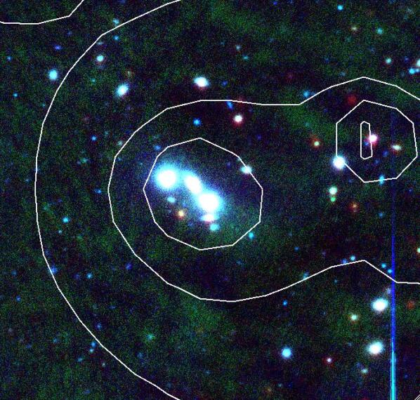
Figure 1: An example image of one of the 12 extended X-ray sources unambiguously associated with a $z<0.8$ cluster on the basis of visual inspection. The image is composed of $rz3.6\micron$ data and is 2′ on a side with standard astronomical orientation. The white contours indicate X-ray emission.

This simple sifting can work to at least $z=1.2$ as the highest redshift XMM-LSS cluster XLSSC 046 (Bremer et al., 2006) is straightforwardly selected in this way with an obvious compact overdensity of $3.6\micron$ galaxies at the X-ray position with no bright optical counterparts (see Figure 2). However, at high redshifts whether a cluster is straightforwardly identifiable depends on several factors affecting its surface density contrast against the background and foreground galaxies. If the foreground/background density in the $z=1.2$ cluster field had been higher and the spatial distribution of red cluster galaxies less compact (spread over a 1′ radius region rather than the 15″ radius of the detected overdensity), the system would have been harder to discern in this way.

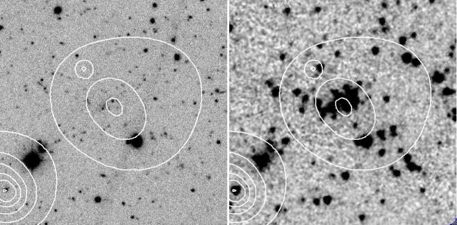
Figure 2: A comparison of the appearance of the confirmed $z=1.2$ cluster XLSSC 046 in $r$-band (left panel) and the 3.6µm waveband (right panel). Each image is approximately 2′ on a side with standard astronomical orientation. The white contours indicate X-ray emission.

Two exceptions to this process are clusters 06 and 19. Cluster 06 lies at the very edge of the SWIRE footprint and has data available at 3.6µm but not 4.5µm. Cluster candidate 19 lies just outside the SWIRE footprint yet had previously been flagged as a high redshift candidate on the basis of the extended X-ray image and faint, $i$-band detection of the candidate BCG. We include it in the following discussion and in Table 1 yet do not include it in the number of systems quoted in the $z>0.8$ area limited sample.

The visual classification supported by the existing spectroscopic observations populates each cluster class as follows: spectroscopically confirmed or candidate clusters at $z<0.8$, 57 (“$z<0.8$ clusters” hereafter); spectroscopically confirmed clusters at $z>0.8$, 9 (see Figure 3; “confirmed clusters” hereafter); candidate clusters at $z>0.8$, 14 (see Figure 4; “candidate clusters” hereafter); point-like or marginal sources with no clear identification, 8, (see Figure 6; “unknown extended sources” hereafter).

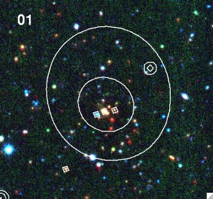
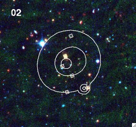
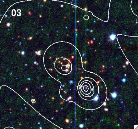
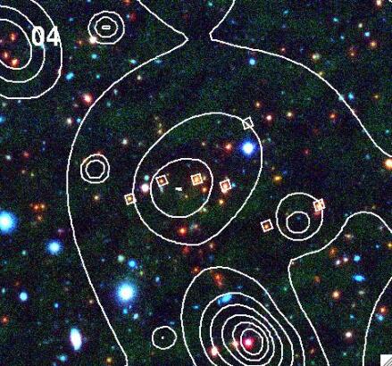
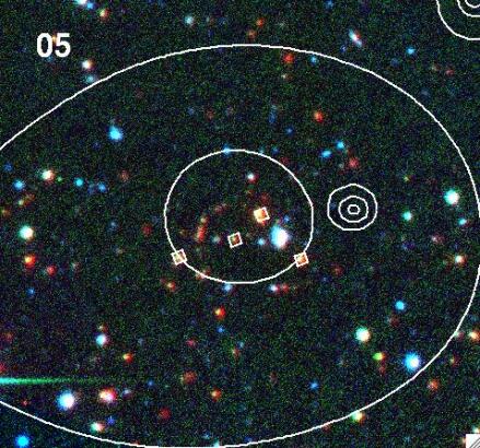
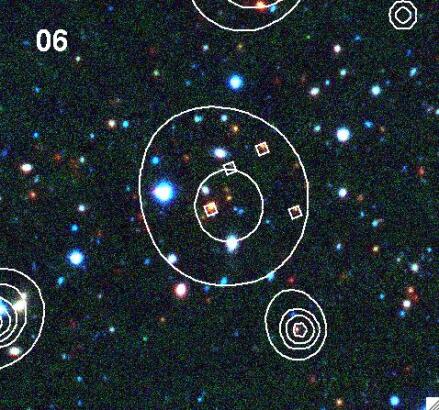
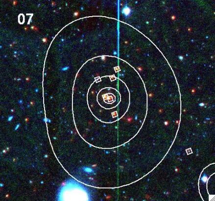
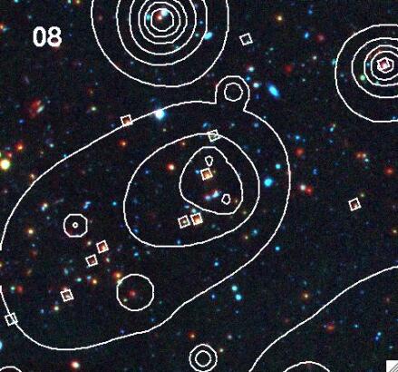
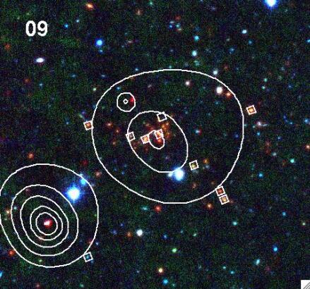
Figure 3: Colour images of spectroscopically confirmed clusters (see Table 1). Images are composed of $rz3.6\micron$ data. The white squares indicate spectroscopically confirmed galaxies at the cluster redshift. The white contours indicate X-ray emission. Images are 2′ on a side with standard astronomical orientation.

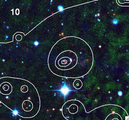
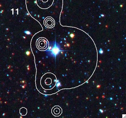
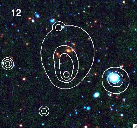
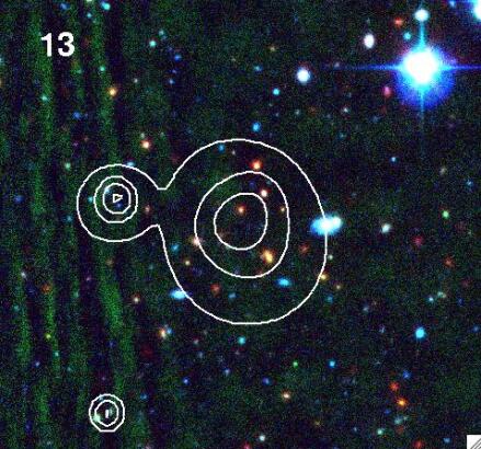
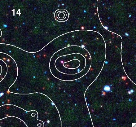
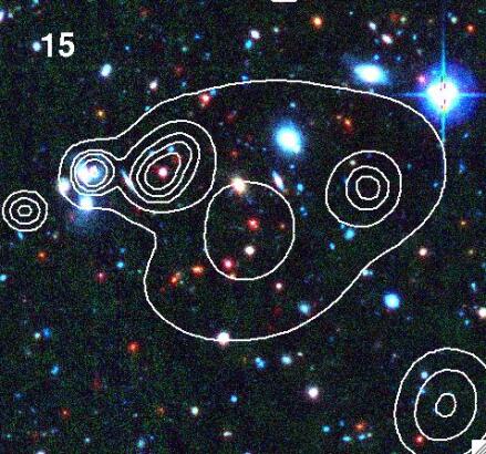
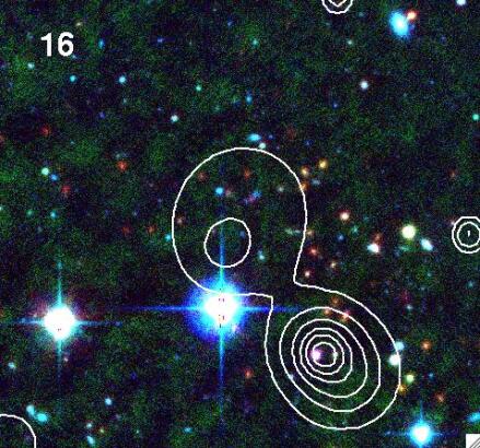
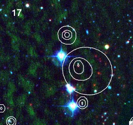
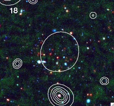
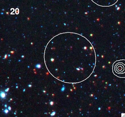
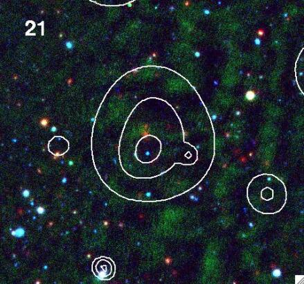
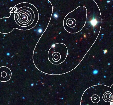
Figure 4: Colour images of candidate clusters (see Table 1). Images are composed of $rz3.6\micron$ data. The white contours indicate X-ray emission. Images are approximately 2′ on a side with standard astronomical orientation.

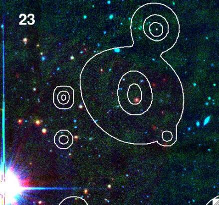
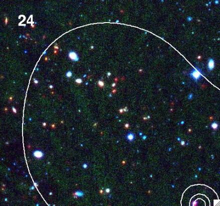
Figure 5: continued

Colour images of candidate clusters (see Table 1). Images are composed of $rz[3.6\micron]$ data. The white contours indicate X-ray emission. Images are 2′ on a side with standard astronomical orientation.

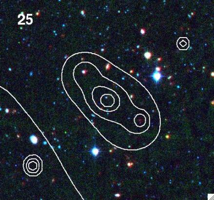
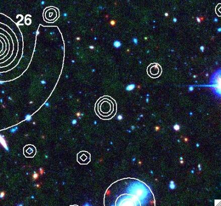
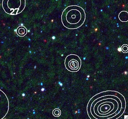
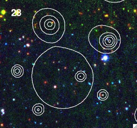
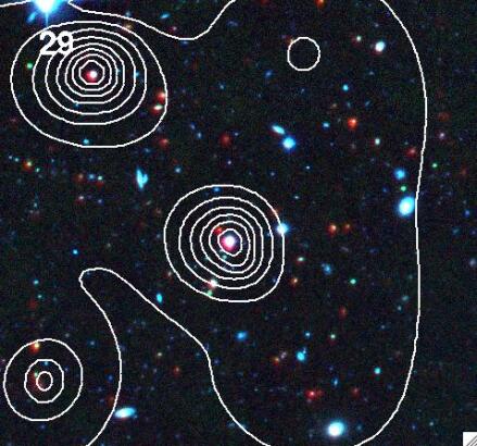
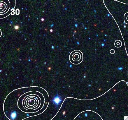
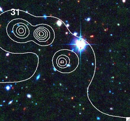
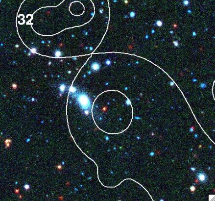
Figure 6: Colour images of marginal or unknown extended X-ray sources (see Table 1). Images are composed of $rz3.6\micron$ data. The white contours indicate X-ray emission. Images are 2′ on a side with standard astronomical orientation.

3.2 The surface density of faint, red galaxies

Following the visual inspection, the colours of galaxies in all fields, whether or not identified as clustered from initial inspection, are examined in order to identify any clustering in both position and colour. These colours, given data of suitable depth, can provide an indication of the redshift of the system.

The photometric analysis employs the $r-3.6\micron$ and $3.6\micron-4.5\micron$ colours derived from the CFHTLS and SPITZER/IRAC data. These colours have been proven to select for distant cluster galaxy populations (see Papovich, 2008; Muzzin et al., 2008). With data of sufficient depth, the use of the $3.6\micron-4.5\micron$ colour is particularly powerful as it is a strong function of redshift between $0.5<z<1.5$ for galaxies with a wide range of star formation histories and the scatter in colour between histories is relatively small (see Papovich, 2008). For all clusters, the surface density of galaxies within 1′ of the X-ray position with $r-3.6\micron>3$ and (independently) $r>22$ and $3.6\micron-4.5\micron$$>-0.1$ was computed. For 3.6µm sources that are undetected in $r$ (approximately $r>25.9$) the computed colour is a lower limit on the true colour. These values were compared to those computed for the $z<0.8$ clusters and 1000 randomly placed apertures over the survey area. Figure 7 displays these values for all C1 and C2 clusters and cluster candidates in the 9 deg²  area. As expected, the spectroscopically confirmed distant clusters are in the top-right of the distribution, along with many of the candidates. This is evidence that at least a subset of the candidates are at redshifts similar to, or even higher than, those of the spectroscopically confirmed clusters, with the candidate fields having a higher surface density of sources with the reddest $3.6\micron-4.5\micron$ colours than the spectroscopically confirmed $z>0.8$ clusters.

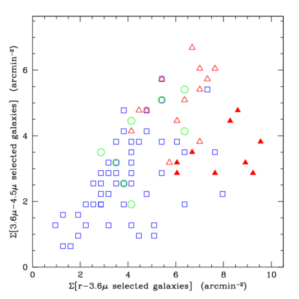
Figure 7: The surface density of galaxies selected according to the photometric criteria described in the text and located within 1′ of the X-ray centroid. Sources are classified as $z<0.8$ (blue squares), $z>0.8$ spectroscopically confirmed clusters (solid red triangles), $z>0.8$ candidate clusters (open red triangles) and unknown sources (green circles).

The separation of cluster classes indicated in Figure 7 is supported by a two-sided Kolmogorov-Smirnov (KS) analysis of the surface density values (in this case using $r-3.6\micron$ colours). A KS test between the $z<0.8$ cluster sample and the 1000 random apertures result in a probability that the two samples are drawn from the same population of 0.74, which is sensible given the photometric criteria are designed to be sensitive to $z>0.8$ galaxies. The corresponding KS probabilities between the $z>0.8$ sample (confirmed and candidates) and the $z<0.8$ clusters, the random apertures and the unknown sources are $5\times 10^{-4}$, $5\times 10^{-5}$ and $4\times 10^{-2}$ respectively – thus confirming the trend observed in Figure 7.

However, some overlap remains between the visually-assigned classes. For the low- versus high-redshift sources this is partly due to the fact that photometric uncertainties will result in low redshift galaxies exceeding the applied colour cut and vice versa – this blurring is expected to be most evident for clusters close to the effective redshift cut-off implied by the photometric criteria. In addition, while it is unlikely that any of the 57 $z<0.8$ clusters are at $z>0.8$ we do note that two of the $z>0.8$ candidate clusters ultimately result in photometric redshift estimates slightly less than $z=0.8$. In general though, when considering the $z>0.8$ candidate clusters and the unknown extended sources the surface density analysis indicates that the optical-MIR data cannot provide an unambiguous assessment of these systems. Put another way, there is no straightforward threshold that can be applied to the surface density of optical-MIR selected galaxies along the line of sight to the extended X-ray source sample that will generate a complete sample of candidate distant cluster candidates with low contamination. We address this point further in Section 4.

3.3 Identifying cluster red sequences

In addition to computing the surface density of faint, red galaxies, colour magnitude diagrams (CMDs) and colour histograms in both $r-3.6\micron$ and $3.6\micron-4.5\micron$ were created for the confirmed and candidate $z>0.8$ clusters and compared to the background colour distribution (e.g. see Figure 8). Assuming that a cluster contains a significant number of passively-evolving galaxies, the presence of a red sequence should confirm a cluster identification and the characteristics of that sequence should indicate an estimated redshift for the cluster when compared to stellar population models (Figure 9). The analysis indicates that the confirmed clusters, located at $0.8<z<1.2$, display red sequence colours broadly consistent with the expectation of a simple model of an old, passively evolving stellar population considered at the confirmed spectroscopic redshift (see Figure 9 for further details). A number of the candidate clusters at $z>0.8$ also display red sequences consistent with the expectation of a high redshift passive stellar population. However, it is also clear that a subset of the candidate clusters do not display red sequence colours consistent with this simple model of a high redshift stellar population – specifically they appear to be systematically bluer in $r-3.6\micron$ than the expected colour for $1<z<2$. This effect can be understood by noting (as indicated in Figure 8) that a number of sources detected at 3.6µm in the candidate clusters are undetected in CFHTLS W1 $r$-band data. The indicated $r-3.6\micron$ red sequence colours are therefore lower limits and will underestimate the true colour. A further limitation is that the $3.6\micron-4.5\micron$ red sequence colour is largely degenerate with redshift at $z\ga 1.3$. The above steps indicate (often strongly) that each confirmed and candidate cluster is associated with an overdensity of galaxies consistent with $z>0.8$. However, although the optical and MIR imaging data are effective at determining the presence of over-densities of high-redshift galaxies they only provide limited information on the redshift associated with the red sequence location.

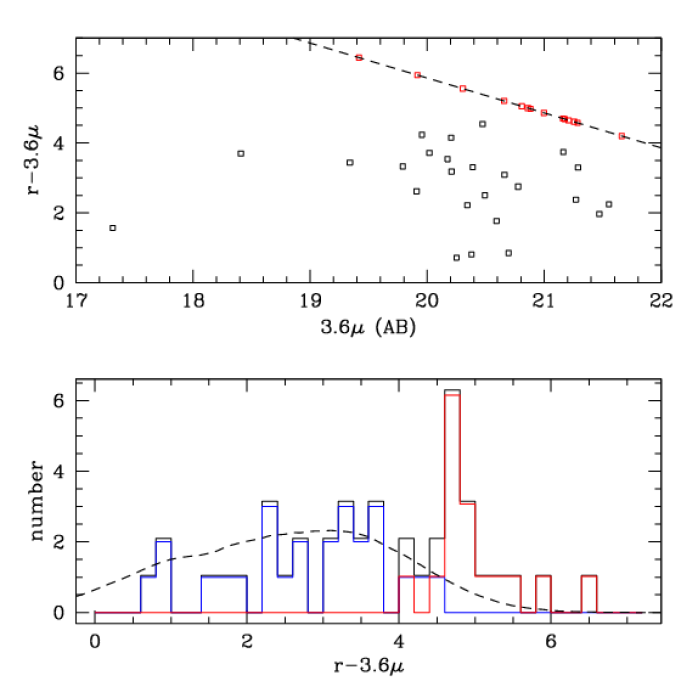
Figure 8: Optical-MIR photometry for cluster candidate 21. All sources within 1′ of the X-ray position are indicated. Top panel: red points indicate sources undetected in $r$. Bottom panel: the histograms indicate sources detected in $r$ (blue), undetected in $r$ (red) and total source counts (black). Each histogram is scaled to be visible in overlay. The dashed line shows the background colour distribution. This is formed by computing the colour histogram of all sources more than 1′ away from each C1$+$C2 source in the sample. The histogram amplitude is then scaled by the ratio of the areas of the cluster and background areas.

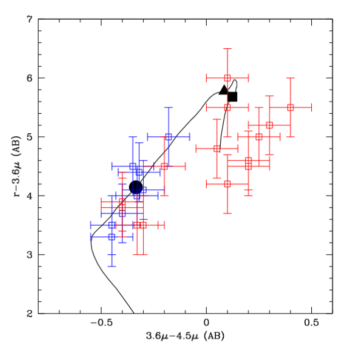
Figure 9: The distribution of cluster red sequence locations in the $r-3.6\micron$ and $3.6\micron-4.5\micron$ plane. Blue points indicate spectroscopically confirmed clusters at $z>0.8$ and red points indicate candidate clusters at $z>0.8$. Errors are fixed at 0.1 mag. in $3.6\micron-4.5\micron$ and 0.5 mag. in $r-3.6\micron$. The black line indicates the locus followed by a passively evolving 1 Gyr solar metallicity burst of star formation occuring at $z_{f}=5$ (Bruzual & Charlot, 2003). The colour of this model stellar population at redshifts 1, 1.5 and 2 are indicated respectively by the black circle, triangle and square.

3.4 Photometric redshift analysis

Having searched for evidence of red sequences in colour magnitude diagrams (CMDs), we extend our analysis by removing the assumption that any distant cluster galaxy population has a significant red sequence, and allow the possibility that the galaxies associated with a cluster can have a range of spectral energy distributions corresponding to a range of star formation histories.

We use the public code Le Phare (Arnouts et al., 2002; Ilbert et al., 2006) to estimate the photometric redshifts. Le Phare is based on a standard template fitting procedure. The templates are redshifted and integrated through the appropriate transmission curves. The photometric redshifts are obtained by comparing the modelled fluxes and the observed fluxes with a $\chi^{2}$ merit function. We run the code using exactly the same configuration as used in the COSMOS field (Ilbert et al., 2009). The set of templates was generated by Polletta et al. (2007) for the elliptical and spiral galaxies. Twelve blue templates generated with Bruzual & Charlot (2003) were added. Four different dust extinction laws were applied (Prevot et al., 1984; Calzetti et al., 2000), and an additional bump at 2175Å, depending on the considered template. Emission lines were added to the templates using relations between the UV continuum, the star formation rate and the emission line fluxes (Kennicutt, 1998). Moreover, an automatic calibration of the zero-points was performed using a sample of 650 spectroscopic redshifts within the photometric data area drawn from the XMM-LSS sample described by Adami et al. (2011). The calibration is obtained by comparing the observed and modelled fluxes (Ilbert et al., 2006) at known spectroscopic redshifts.

Having demonstrated that the optical and MIR colours of candidate $z>0.8$ galaxies provide only a relatively inaccurate estimate of the redshift of a given confirmed or candidate cluster, the photometric redshift analysis described here is limited to those confirmed and candidate clusters with additional NIR photometry in at least the $J$ and $K_{s}$ bands (see Table 1 for a list of clusters with $JK$ photometry). At $z>0.8$ the $JK$ bands sample the rest frame optical spectral energy distribution (SED) including the prominent D4000 feature which provides a strong $JK$ colour signature – and thus strong constraining power in a photometric redshift analysis – as a function of redshift for galaxies composed of evolved stellar populations. Figure 10 displays the photometric redshift histograms for all clusters with available $JK$ data. For clusters with spectroscopic redshifts, data are plotted for all galaxies within 30″ of the X-ray source that are brighter than the $K_{s}$-band completeness limit of each data set (see Section 2.2). For clusters with photometric redshifts (see below) $z_{phot}<1.2$ and $z_{phot}>1.2$, data are plotted for all galaxies within 1′ and 30″ respectively of each X-ray source that are brighter than the corresponding $K_{s}$-band completeness limit.

We represent the redshift density function for each cluster using both a standard histogram ($\delta z=0.1$) and a variable kernel density estimation (VKDE) approach. The VKDE approach represents the contribution of each galaxy to the redshift density function as a Gaussian of width $\sigma=0.03\times(1+z)$ and unit area. A first estimate of the photometric redshift of each cluster is determined by identifying visually the peak associated with the X-ray source in Figure 10. We then compute the cluster photometric redshift as the mean of the VKDE-weighted redshift distribution, i.e.

$${z_{cluster}=\frac{\int z~{}K(z)~{}{\rm d}z}{\int K(z)~{}{\rm d}z}}$$ (1)

over the local interval where the VKDE distribution $K(z)$ exceeds $0.5\times K(z_{peak})$. The resulting $z_{cluster}$ for all candidate clusters is displayed in Table 1. For the five spectroscopically confirmed clusters with NIR data coverage we can compute the effective photometric redshift error of this method as

$${\sigma_{z}=\left[\frac{1}{N}\sum\left(\frac{(z_{spec}-z_{phot})}{(1+z_{spec})}\right)^{2}\right]^{1/2}}$$ (2)

which yields $\sigma_{z}=0.025$. This error will naturally increase as one extends this approach to the candidate clusters which typically represent less clear redshift peaks composed of smaller numbers of galaxies. Figure 10 also displays photometrically selected cluster galaxies in field of each cluster. Cluster galaxies are selected as occupying the local interval $K(z)>0.5\times K(z_{cluster})$. Figure 10 further displays the $J-K_{s}$ CMD for photometrically selected members of each cluster.

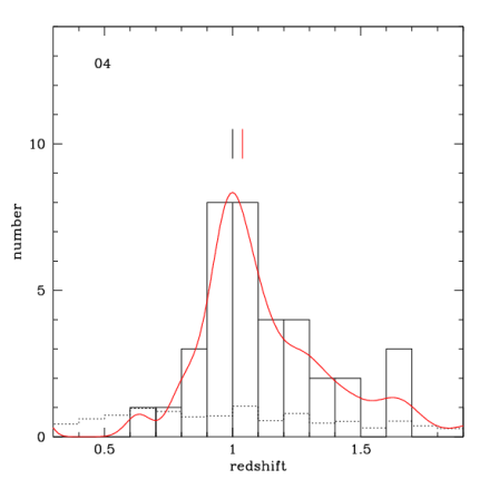
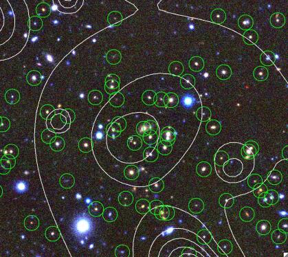
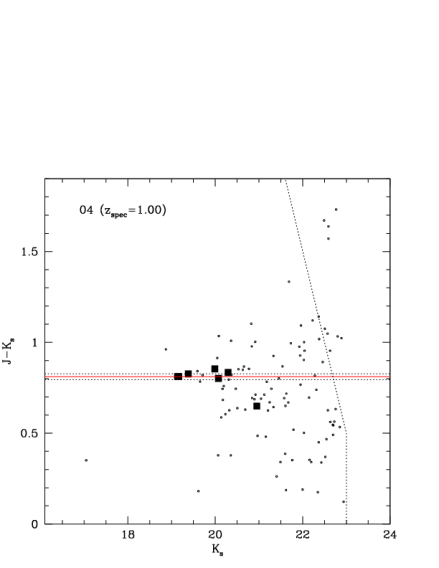
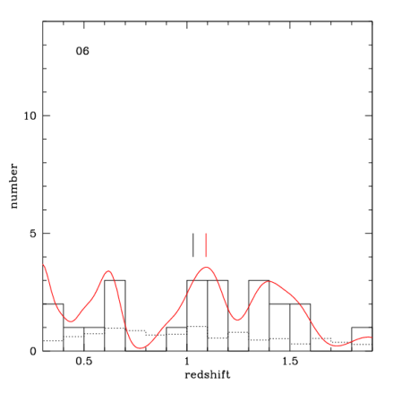
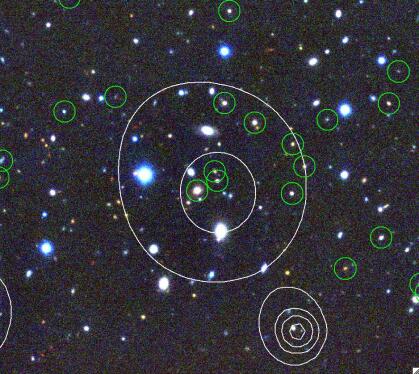
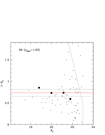
Figure 10: Photometric redshifts and NIR photometry for each cluster with available $JK$ data (see text for additional information). Left panel: photometric redshift histogram for all sources located close to each X-ray cluster centroid. The red curve indicates the VKDE distribution and the dotted line is the appropriately scaled background. The vertical red tick mark indicates the computed photometric redshift for each cluster. For spectroscopically confirmed clusters the vertical black tick mark indicates the spectroscopic redshift. Middle panel: $iJK$ image of each cluster. Each image is 2′ on a side and follows standard astronomical orientation. The white contours indicate the X-ray emission in each field and the green circles indicate photometrically selected cluster members. Right panel: colour magnitude diagram for sources within 1′ of each cluster X-ray centroid. For spectroscopically confirmed clusters the black squares indicate spectroscopically selected cluster members. For candidate clusters the black squares indicate photometrically selected members. Points indicate all other sources. The horizontal red and dotted black lines indicate the computed red sequence location and associated uncertainty. The angled dotted line indicates the photometric completeness in each field.

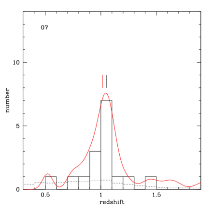
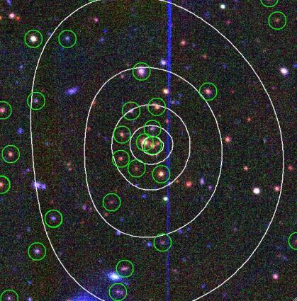
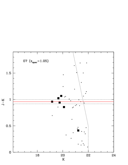
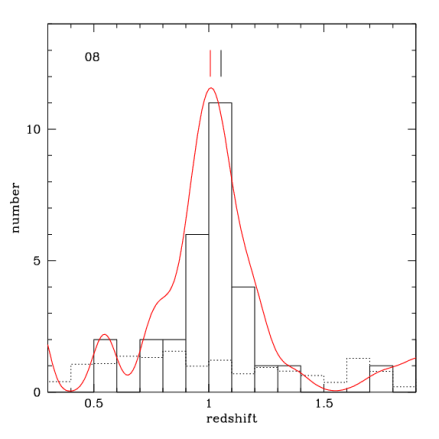
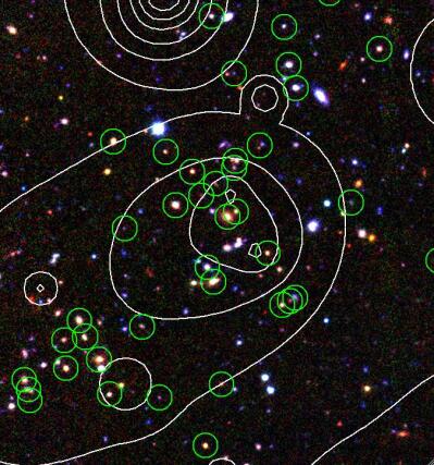
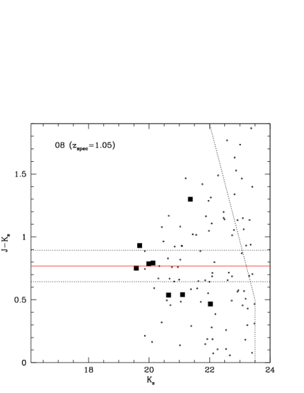
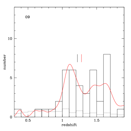
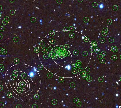
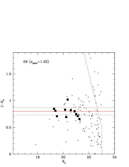
Figure 11: continued

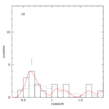
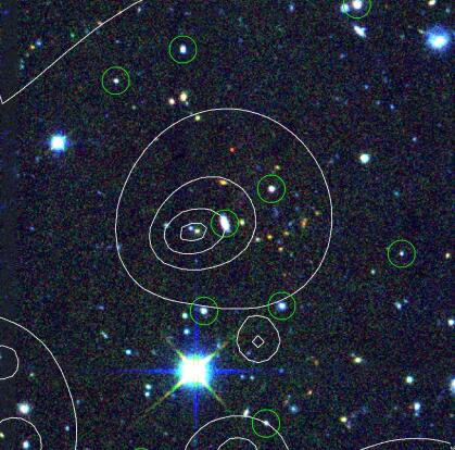
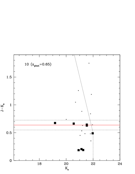
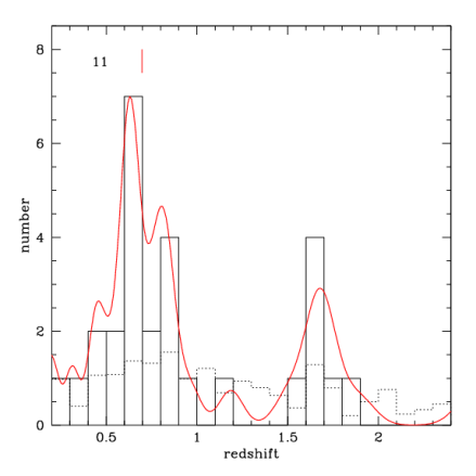
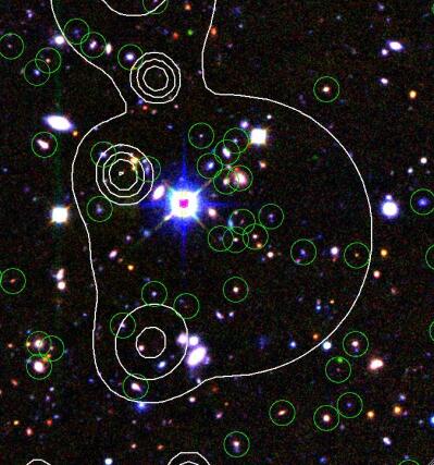
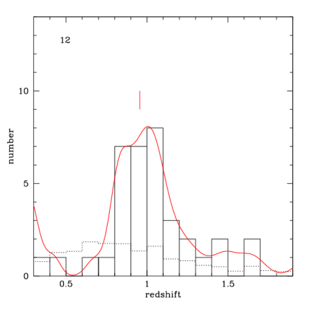
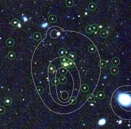
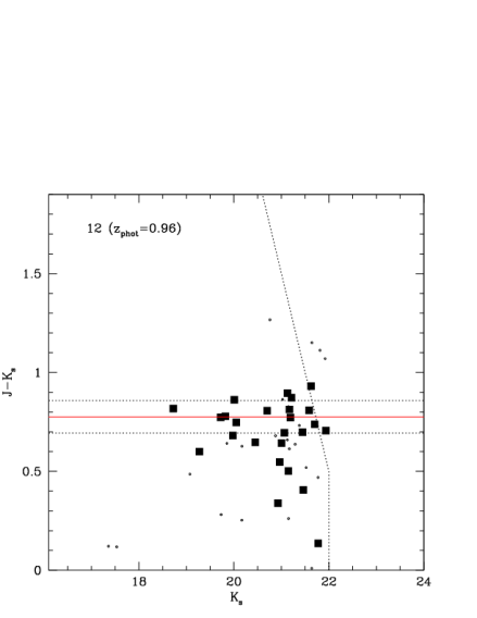
Figure 12: continued

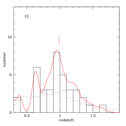
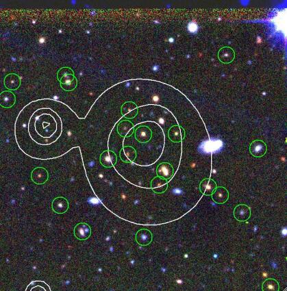
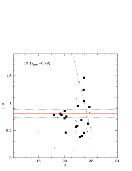
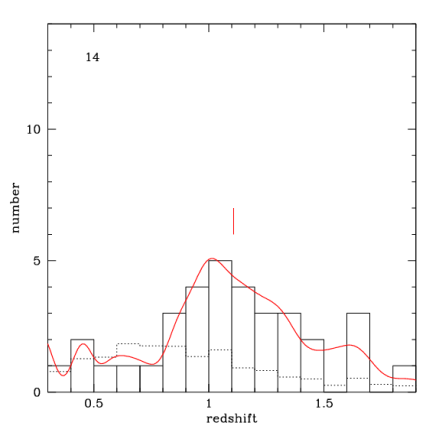
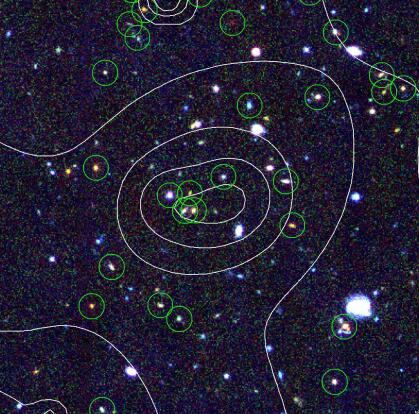
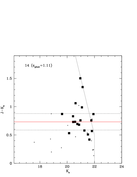
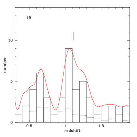
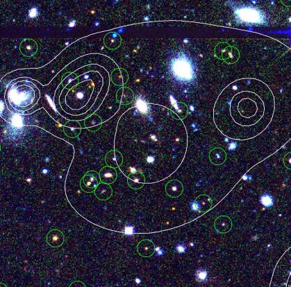
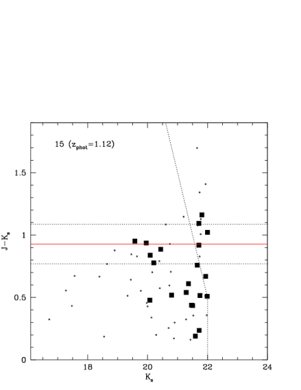
Figure 13: continued

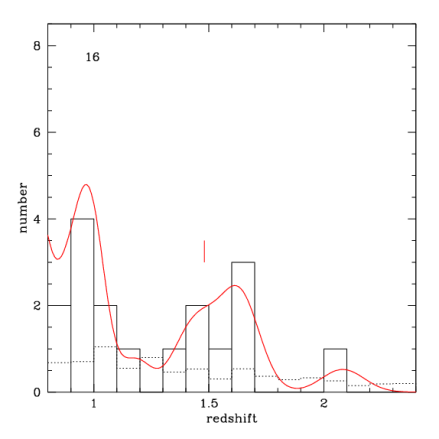
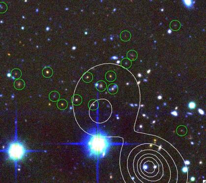
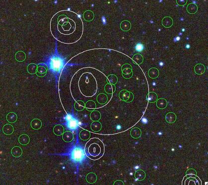
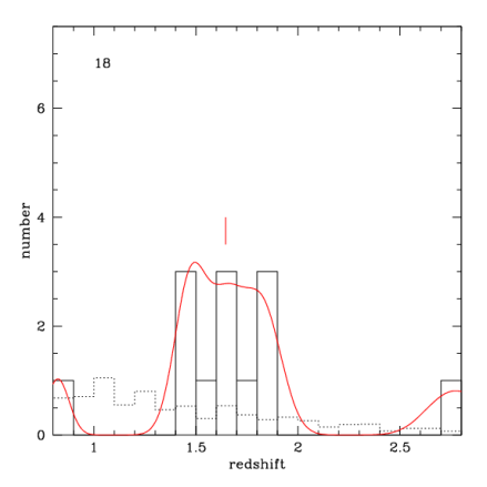
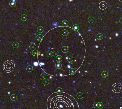
Figure 14: continued

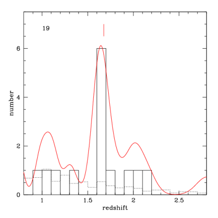
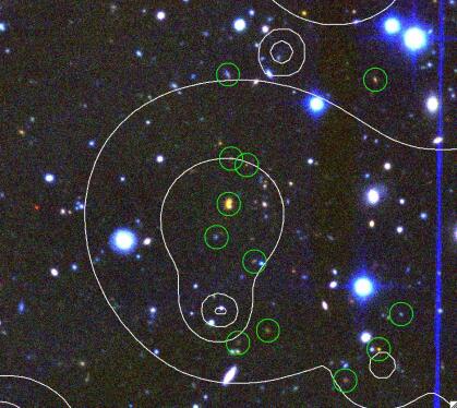
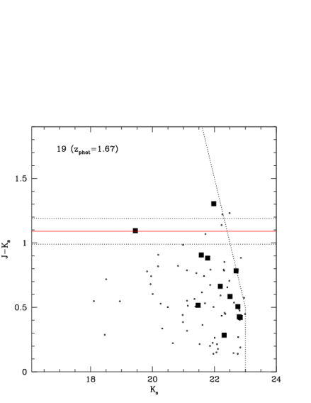
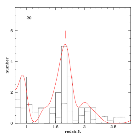
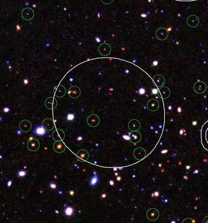
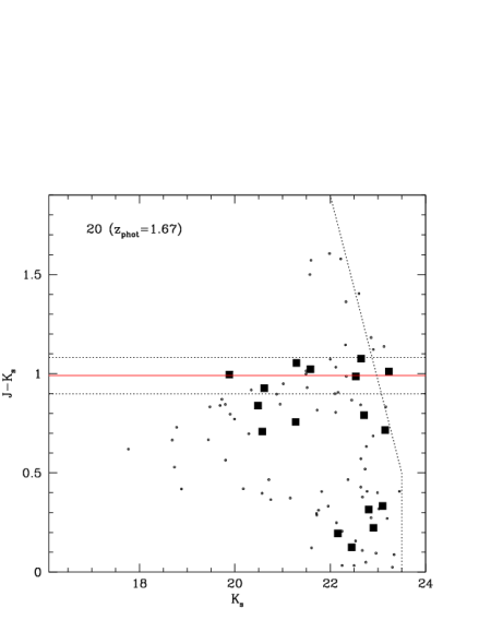
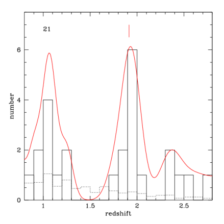
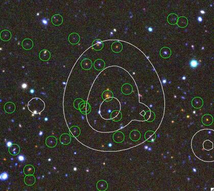
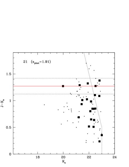
Figure 15: continued

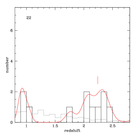
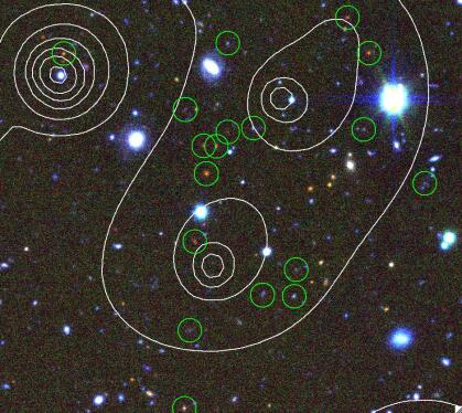
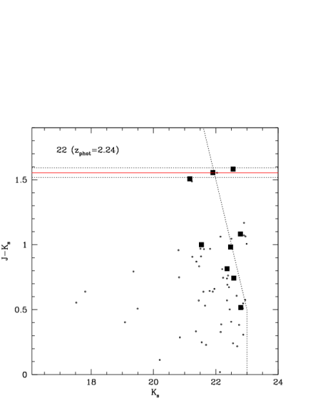
Figure 16: continued

4 Discussion

4.1 Cluster red sequences: implications for galaxy assembly history

In Section 3.3 we investigated the limitations of the $r-3.6\micron$ and $3.6\micron-4.5\micron$ data in the determination of the location of cluster red sequences. We return to this issue with the NIR data and the results of the photometric redshift analysis in hand and investigate two approaches to compute the colour sequence of cluster member galaxies selected by a) photometric redshift and 2) statistical background subtraction on the NIR colour magnitude plane.

4.1.1 Computing the red sequence colour employing photometric redshifts

Figure 10 displays the CMDs of cluster galaxies in confirmed and candidate clusters selected by photometric redshift (or spectroscopic redshift if available) and proximity to the X-ray source. In order to identify the location of any red sequence in each cluster we apply the method outlined by Fassbender et al. (2011) whereby one identifies the third reddest galaxy in each CMD (3RG) and selects galaxies displaying $J-K_{s}$ colours within $\rm 3RG\pm 0.3$. We then compute the cluster “red sequence” colour as the median of this set of galaxies ($C_{med}$) and the spread as either the colour of the galaxies enclosing 68% of the distribution (i.e. $\sigma_{c}=0.5\times[C_{84}-C_{16}]$; for $N>3$) or the full colour range (for $N\leq 3$). We apply this method to all confirmed and candidate clusters with $J-K_{s}$ imaging and display the resulting $C_{med}$ and $\sigma_{c}$ values in Figure 17. For cluster 19 we set $C_{med}$ equal to the colour of the candidate BCG and $\sigma_{c}=0.1$. In many cases this approach identifies a viable, yet often poorly populated, red sequence. However, we note that this approach does not identify a clear red sequence for candidate clusters 16, 17 and 18. We address this result in more detail in the Section 4.1.2.

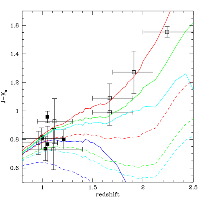
Figure 17: Cluster red sequence colour computed for spectroscopically confirmed (solid squares) and candidate (open squares) clusters. The colour-redshift data are compared to model predictions generated using the BC03 spectral sysnthesis code (Bruzual & Charlot, 2003). Each model features either a 1 Gyr burst (solid line) or $\tau=1$ Gyr (dashed line) solar metallicity stellar population with a standard Salpeter IMF. Models are displayed for formation redshifts of 10 (red), 5 (green), 4 (cyan) and 3 (blue) respectively.

For those clusters displaying a clear red sequence consistent with $C_{med}$ and $\sigma_{c}$ we compare the red sequence colour versus redshift data to a set of representative colour-redshift loci generated using the BC03 spectral synthesis code (Bruzual & Charlot, 2003). The plot indicates that the location of the putative red sequences of the confirmed and candidate clusters follow a clear locus in colour-redshift space that can be described by the simple passive evolution of an old stellar population. We do not attempt to fit the stellar population parameters best describing the data beyond noting that solar metallicity models arising from a 1 Gyr burst of star formation at $z_{f}>5$ appear to be favoured over either extended ($\tau=1$ Gyr), sub-solar ($Z=0.4Z_{\odot}$) or younger ($z_{f}<5$) bursts of star formation. It is worth noting at this point that the strength of this conclusion rests upon the red sequence colours of the candidate clusters at $z>1.5$. In one sense this demonstrates the important leverage that distant clusters place upon our knowledge of galaxy evolution in dense environments. In another sense however, this result can only be viewed as tentative pending spectroscopic confirmation of these clusters.

4.1.2 Computing the red sequence location employing background subtraction on the CMD plane

An alternative approach to identifying the red sequence of candidate cluster galaxies is to investigate their distribution directly on the colour magnitude plane. The main issue is to isolate the potentially weak cluster signature from the “background” of non-cluster galaxies along the line of sight. To achieve this we bin the colour magnitude distribution of galaxies located within 1′ of each cluster X-ray centroid. Galaxies are binned on the $J-K_{s}$ versus $K_{s}$ plane with bin dimensions of 0.2 and 0.5 mag. respectively. The CMD of non-cluster galaxies (termed the model background here) is formed by selecting all sources at $>1\arcmin$ from each cluster or cluster candidate and scaling the resulting distribution by the relative cluster and background sky areas.

Although the resulting background subtracted CMD for each cluster displays an identifiable overdensity of faint, red galaxies, the signal is accompanied by variations in the true background associated with each cluster (both Poisson and cosmic in nature). Upon subtraction of the scaled model background these variations persist as residual positive and negative signatures. However, their statistical distribution should average to zero over all cluster fields and, in an attempt to reduce their impact, we stack the binned subtracted CMDs to investigate the average cluster CMD. Prior to stacking we shift each cluster distribution on the colour magnitude plane to account for the $k$-correction and distance dimming of an evolving stellar population at each cluster redshift. We correct each cluster to a common redshift applying an apparent colour and magnitude shift based upon the evolution of a 1 Gyr solar metallicity burst of star formation occuring at $z_{f}=10$ and described by a Salpeter IMF. Using this same model we have confirmed that the colour terms between the different NIR filter systems employed are small compared to the photometric zero point errors for each cluster. We stack all cluster and cluster canditates as follows: spectroscopically confirmed clusters at $z>0.8$ (5 systems), cluster candidates at $0.8<z_{phot}<1.2$ (4), cluster candidates at $z_{phot}>1.2$ either with a clear red sequence (4) or without (3, i.e. clusters 16, 17 and 18). We also stack the CMD of six control fields constructed in order to test the null hypothesis that each cluster candidate is false. We take the location of six clusters observed with HAWK-I and shift the cluster centroid to an adjacent detector (approximately a 3′ shift). We then repeat the stacking procedure using these new centroids and apply the same colour and magnitude shifts applied to galaxies selected according the original cluster locations.

Figure 18 displays the colour histrogram generated from each stack by summing the CMD along the magnitude axis with the restriction $K_{s}<22.5$, for $J-K_{s}<0.5$, or $K_{s}<23.0-(J-K_{s})$ otherwise, to consider the photometrically complete region of the CMD. Figure 18 confirms that there is little difference in the intrinsic red sequence properties between spectroscopically confirmed clusters at $z\sim 1$ and the candidate clusters. More importantly, the subset of candidate clusters lacking apparent red sequences on the basis of photometric redshift selection have been shown to have average red sequences statistically identical to the remainder of the candidate sample following the stacking analysis. We speculate that these clusters display a range of star formation histories that are not well described by the available SED templates used in the photometric redshift analysis. The resulting photometric redshift peak will be broadened by this systematic uncertainty and attempting to select cluster galaxies using the photometric redshift method described in this paper will result in a greater level of background contamination relative to clusters with well modeled SEDs. Thus the already weak red sequence may be diluted further by the increased effective background along these sightlines. This effect can only be verified once spectroscopic redshifts are available for these clusters. All of the stacked cluster colour distributions are clearly real and significant when compared to the null distribution. For the clusters without an individual red sequence the fact that only 3 systems contribute to the average supports the assertion that the majority (if not all) are real as otherwise the signal observed in the average histogram would be very much diluted. We therefore conclude that each of the clusters presented in this sample is real in that the extended X-ray source is associated with a galaxy population clustered both spatially and in colour, whose spectra, photometric redshifts and/or colours are consistent with $z>0.8$.

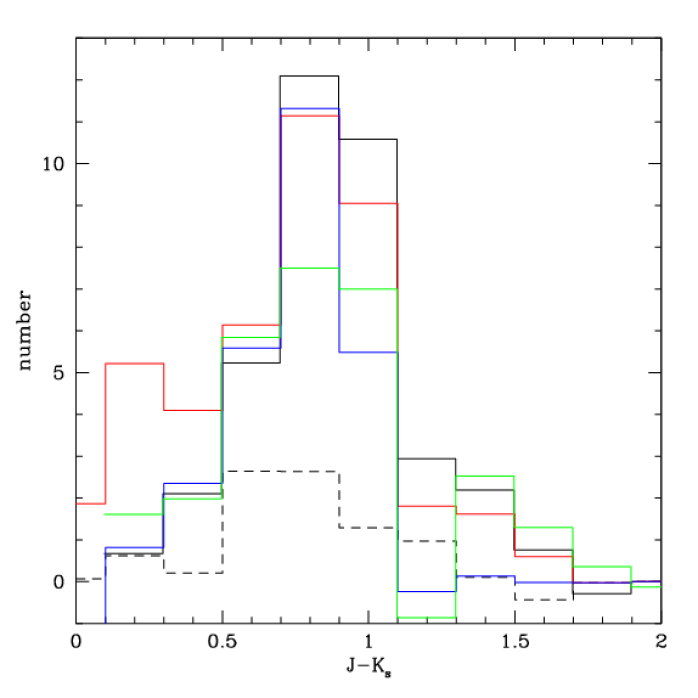
Figure 18: Colour histograms generated by summing over the stacked CMD histograms for each cluster subsample: spectroscopically confirmed clusters (solid black; 5 systems), candidate clusters with $z_{phot}<1.2$ (green; 4 systems), candidate clusters at $z_{phot}>1.2$ with evidence for individual red sequences (red; 4 systems) and without (blue; 3 systems), 6 random locations within the HAWK-I fields (dashed black). The numbers represent the average number of galaxies at each colour brighter than the applied brightness cut. See text for further details.

4.2 The cluster red fraction

The cluster red fraction provides a simple statement of the population mix of cluster galaxy members selected by colour and magnitude. It is conceptually identical to the cluster blue fraction computed by Butcher and Oemler (1984) yet here we focus on the the red galaxy component in order to highlight the contribution of the cluster red sequence to each cluster in our sample. We compute the red fraction as the ratio

$${f_{R}=\frac{N_{R,cluster}-N_{R,back}}{N_{T,cluster}-N_{T,back}}}$$ (3)

where $N_{R}$ denotes the number of galaxies satisfying $J-K_{s}>\rm 3RG-0.3$ and $K_{s}$ brighter than a evolving model early-type galaxy. The model assumes a galaxy of $K_{s}=22.5$ at $z=1.5$ described by a 1Gyr solar metallicity burst of star formation occurring at $z_{f}=10$ and described by a Salpeter IMF. The corresponding $K_{s}$ limit at the redshift of each cluster is computed accordingly. $N_{T}$ denotes the total number of galaxies satisfying the appropriate magnitude limit. $N_{cluster}$ includes all galaxies within 1′ of the X-ray centroid and $N_{back}$ includes all galaxies at greater than 1′ from the cluster centroid with the value scaled to match the relative areas of the cluster and background samples.

The red fraction values for all confirmed and candidate clusters with $J-K_{s}$ photometry are displayed in Figure 19. The figure indicates that the cluster sample displays a range of red fraction values ranging from clusters almost wholly dominated by the red sequence ($f_{R}\sim 1$) to those with low values, i.e. $f_{R}<0.2$. The observation of a wide range of red fraction values supports the assertion that the compilation of a complete sample of X-ray selected distant clusters can provide a relatively unbiased view of galaxy populations in such systems. A comparable analysis of the red fractions in a non-X-ray selected distant cluster sample has not yet been performed – which is unfortunate as the results of such a study would provide a valuable perspective on the wavelength dependent biases affecting distant cluster identification.

The range of red fraction values displayed by the distant cluster sample is similar in extent to that of comparable mass clusters at redshifts $z\sim 0.3$ (Urquhart et al., 2010) also studied within the XMM-LSS survey (note that we discuss mass estimation based upon X-ray flux measurements in Section 4.3). However, the XMM-LSS distant clusters will increase in mass by a factor $\sim 5$ between a redshift $z=1.5$ and $z<0.3$ (Boylan-Kolchin et al., 2009). Such low redshift clusters of mass $>5\times 10^{14}\rm M_{\odot}$ typically display dominant, bright red sequence populations with $f_{R}>0.8$. If one assumes that the evolution of galaxies onto the red sequence occurs following the rapid cessation of star formation (quenching) – for example as a result of ram pressure stripping (Gunn and Gott, 1972) or galaxy-galaxy interactions (Dressler et al., 1994) – then the large observed range of red fraction values displayed by the XMM-LSS distant cluster is consistent with the scenario whereby the galaxy populations have been caught in a variety of states transforming between active star forming environments (where the red fraction is low and comparable to that of the field) to a “red and dead” environment typified by $z<1$ massive clusters.

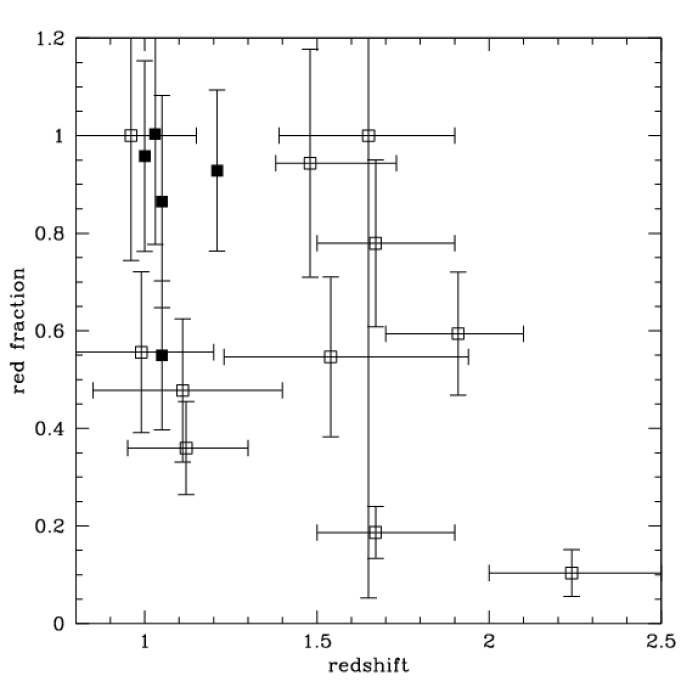
Figure 19: The red fraction for all confirmed (solid squares) and candidate (open squares) $z>0.8$ clusters with $J-K_{s}$ photometry. Error bars on the red fraction are Poissonian.

4.3 X-ray fluxes and cluster masses

A key motivation for identifying the most distant clusters is to determine their global properties and thereby reveal the details of cluster evolution. One of the most important properties is the total cluster mass. Unfortunately, this is not observable directly but it can, with certain assumptions, be determined from other observables including the X-ray flux (luminosity) of a system. While one could employ well-studied scaling relations at $z<1$ in order to convert a flux measurement to one of mass, the extrapolation of these scaling relations to $z>1$ is fraught with uncertainty. We therefore adopt an alternative approach whereby we compare the X-ray flux observed from clusters of known redshift (either spectroscopic or photometric) to the flux expected from a model cluster of specified properites. This approach offers the reassurance that the model assumptions are defined and compared to the two observables (flux and redshift) in as clear a manner as possible.

Figure 20 compares the flux values for individual clusters to the flux of model clusters computed as a function of cluster mass and redshift. The model assumes the luminosity-temperature relation of Arnaud & Evrard (1999) with self-similar evolution. The mass-temperature relation is taken from Arnaud, Pointecouteau & Pratt (2005) with $\delta=200$ and massive clusters (extrapolated down to the entire mass range) with self-similar evolution. A comparison of the flux values for the individual clusters to the model indicates that the clusters display an approximate mass limit of $6\times 10^{13}$ to $1\times 10^{14}\rm M_{\odot}$. All clusters display masses inferred from this comparison less than $4\times 10^{14}\rm M_{\odot}$. We refer to this as the baseline model in the following text.

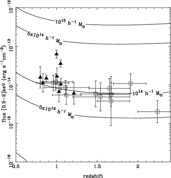
Figure 20: X-ray flux measurements for clusters with confirmed spectroscopic redshifts $z>0.8$ (filled triangles) and candidate clusters with photometric redshifts $z_{phot}>0.8$ (open squares). The contours indicate the expected flux versus redshift properties of model clusters of given mass (see text for details).

It is clear that adopting a different set of model assumptions will affect the mass estimates returned by the above analysis. Figure 21 examines the extent to which adopting an alternative set of scaling relations influences the estimated cluster mass. We retain the assumption that scaling laws evolve in a self-similar manner and compare two alternative approaches to our baseline model described above (Figure 21; black solid lines): 1) a model which replaces the $M_{200}-T$ relation for a $M_{500}-T$ relation taken from Sun et al. (2009), valid down to 1 keV, and assuming the $L_{500}-T$ relation described by Pratt et al. (2009), see Figure 21 (blue dotted lines). Model 2) considers the flux-redshift relation for self-similar clusters following the scaling laws described in Vikhlinin et al. (2009) – see Figure 21 (red dashed lines). Each of these alternative models generates mass estimates for clusters of given flux and redshift which are a generally a factor 2 lower than those generated applying the baseline model.

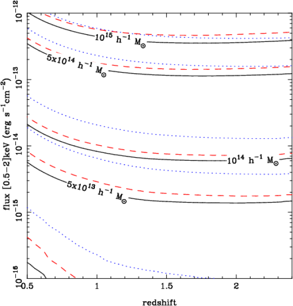
Figure 21: A comparison of the predicted flux versus redshift behaviour of model clusters of varying assumed scaling relations. Black solid lines indicate the baseline model of Arnaud & Evrard (1999) and Arnaud, Pointecouteau & Pratt (2005). Blue dotted lines indicate a model assuming a $M_{500}-T$ relation from Sun et al. (2009) and a $L_{500}-T$ relation from Pratt et al. (2009). The red dashed lines indicate a model employing scaling laws described in Vikhlinin et al. (2009). See text for further details.

Figure 22 examines the extent to which allowing a given scaling relation to evolve with redshift affects the estimated cluster mass. Once again, the black lines in Figure 22 indicate the baseline model described by self-similar evolution. Alternative evolution prescriptions include that of Reichert et al. (2011; blue dots), Clerc et al. (2012; red dashed) and the evolving scaling relations derived by Vikhlinin et al. (2009; green dot-dash). In this case, introducing alternative assumptions regarding the evolution of scaling relations can generate mass estimates for clusters of given flux and redshift which are up to a factor 2-4 greater than those generated applying the baseline model.

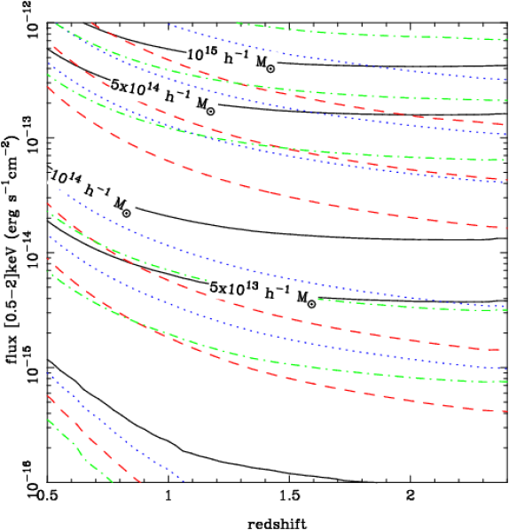
Figure 22: A comparison of the predicted flux versus redshift behaviour of model clusters of varying assumed evolutionary properties. The black solid lines indicate the baseline model described in the text which assumes self-similar evolution. Alternative evolution prescriptions include that of Reichert et al. (2011; blue dots), Clerc et al. (2012; red dashed) and the evolving scaling relations derived by Vikhlinin et al. (2009; green dot-dash).

The above considerations indicate that models which consider potential variations in cluster scaling relations and their evolution can generate mass estimates for $z>0.8$ clusters which vary by up to an order of magnitude. However, given the shape of the contours displayed in Figures 20, 21, and 22 it is apparent that the relative masses of the $z>0.8$ clusters are likely to be robust against uncertainties in the assumed cluster scaling relation model.

4.4 The abundance of distant X-ray selected clusters

Having compiled a sample of $z>0.8$ confirmed and candidate clusters it is instructive to compare their observed abundance to the number predicted using a calculation based upon all relevant cosmological, cluster scaling relation and selection considerations. We computed the expected abundance of distant clusters by assuming a Tinker et al. (2008) redshift-dependent mass function. These authors provide a functional form of the halo mass distribution calibrated using numerical simulations up to $z\sim 2.5$. For this calculation, we assume $\sigma_{8}=0.787$ (Dunkley et al., 2009). Halo masses are then converted from $M_{200b}$ to $M_{200c}$ following Hu & Kravtsov (2003) assuming a NFW mass profile and a concentration model from Bullock et al. (2001). The conversion from masses to X-ray observables is performed based upon the same baseline $M_{200c}-T_{X}$ and $L_{X}-T_{X}$ scaling laws as quoted above. We assume a scatter of $\sigma_{\ln L_{X}|T_{X}}=0.6$ in the $L_{X}-T_{X}$ relation. Both scaling laws are assumed to evolve self-similarly. The XMM-LSS C1+C2 selection function (Pacaud et al., 2006) accounts for the probability of detecting a cluster given its X-ray observables, namely its [0.5-2] keV count-rate and its apparent core radius (corresponding to a $\beta$ model with $\beta=2/3$). For this purpose, model count-rates are estimated assuming an APEC spectral model with abundance $Z=0.3Z_{\odot}$. The core radius is assumed to scale with the halo radius following a simple scaling relation (Clerc et al., 2011): $R_{c}=0.24\times R_{500}$.

The final expected redshift distribution is integrated in various redshift bins: we predict 28.5 clusters lying at $z>0.8$, 5.2 at $z>1.3$ and 2.5 at $z>1.5$ in 9 deg² of surveyed area. By comparison, the sample of high redshift clusters presented in this work consists of up to 22, 7 and 6 clusters at $z>0.8$, $1.3$ and $1.5$ respectively, thus showing a rough agreement with model predictions. However we note a slight ($\sim 2\sigma$) excess of $z>1.5$ clusters in our sample. If confirmed, this excess could be due either to an overestimate of photometric redshifts or to a unaccounted selection bias that would arise due to e.g. an increased contamination of the X-ray flux from unresolved AGNs in these objects. Furthermore, model uncertainties also impact the predicted number of high-redshift clusters. In particular, relaxing the self-similarity constraint on the evolution of the cluster mass-luminosity relation can lead to considerably different predictions (Pacaud et al., 2007).

A further comparison of interest is that between the surface density of XMM-LSS distant clusters and that of other X-ray selected distant cluster samples present in the literature. The surface density of $z>0.8$ clusters in the XMM-LSS survey is $2.3\pm 0.5\,\rm deg^{-2}$ above a nominal mass limit of $\sim 1\times 10^{14}\rm M_{\odot}$. This may be compared to a figure of 15 $z>1.1$ clusters in approximately 1 deg² reported by Bielby et al. (2010) above a mass limit of $\sim 1\times 10^{14}\rm M_{\odot}$ In addition Fassbender et al. (2011) present a compilation of 22 $0.9<z<1.6$ clusters detected in up to 79 deg² of archival XMM observations with a mass limit of $1-2\times 10^{14}\rm M_{\odot}$ (though specific details regarding the selection function are currently unavailable). The surface density of clusters reported in Fassbender et al. (2011) lies between 0.3 and 1.3 $\rm deg^{-2}$ with the exact value depending upon the subset of XMM observations analysed. We note that the Fassbender et al. (2011) compilation containes two previoulsy published XMM-LSS clusters with the result that this comparison is largely but not completely independent.

The variance observed in these reported surface densities arises from differences in the techniques applied to select extended X-ray sources, confirm galaxy overdensities and subsequently compute photometric redshifts or to compile spectroscopic redshifts. A further point worth noting is that distant clusters are often detected in survey data originally compiled to study galaxy clusters at $z<1$. As such, they represent a subset of marginal detections and whether they are subsequently classified and confirmed as distant clusters is a very sensitive function of the set of selection tests applied to the data. With this in mind we have attempted to generate a complete sample of distant X-ray clusters in a manner that depends solely upon the X-ray data by performing an analysis of all extended sources in a subset of the XMM-LSS area. One cannot completely escape the requirement of input from other wavebands, e.g. the optical, NIR and MIR data employed in this paper. However, we have attempted as far as possible to select galaxy overdensities associated with each extended X-ray source in a manner which is insensitive to the assumed star formation history of individual galaxies.

More detailed follow-up of individual clusters, including spectroscopic and deeper X-ray imaging observations are currently underway. Ultimately combining the precise redshift measurements into a self-consistent analysis including selection effects and model uncertainties (Pacaud et al., 2007; Maughan et al., 2012; Reichert et al., 2011; Clerc et al., 2011), we will be able to draw firm conclusions from the abundance of high-redshift clusters.

5 Conclusions

The analysis presented in this paper effectively completes the assessment of 88 extended C1 and C2 sources from approximately 9 deg² of XMM-LSS data. Of these sources 59 display spectroscopic or photometric redshifts $z<0.8$, 21 sources display spectroscopic or photometric redshifts $z>0.8$ (or colours consistent with the same redshift limit in the case of candidate clusters 23 and 24), and a remaining 8 sources appear to be consistent with misclassified point sources or marginal detections. The sample also contains cluster 19 at a photometric redshift $z=1.67$ which is included in this paper having been flagged as a potential distant cluster at an earlier stage. The distant cluster sample is complete in that it represents (with the low-redshift and marginal source identifications) a complete account of a 9 deg² area of the XMM-LSS survey. This sample is generated from the X-ray data employing a quantitative selection function (Pacaud et al., 2006) and it therefore permits a number of important questions in cosmology and galaxy evolution to be investigated.

The complete nature of this sample is dependent upon the primacy of the applied X-ray selection procedures. Although it is difficult to conceive of a targeted X-ray survey for distant clusters that does not employ information at additional wavebands (e.g. optical, MIR, etc.), the application of a simple selection threshold to identify high-significance clusters in these additional wavebands (e.g. the surface density of optical-MIR selected sources) will either lead to an incomplete X-ray sample or a large rate of contamination (from low-redshift or spurious sources), c.f. Figure 7. These comments do not undermine the nature of optical-MIR selected samples of distant clusters – which are complete in terms of the applied selection criteria. Instead they reflect the fact that distant X-ray detected clusters must be confirmed at other wavebands. In doing so with this paper we have attempted to perform as comprehensive an assessment as possible of each confirmed and candidate system with the aim of compiling a complete sample of X-ray selected distant clusters.

It is important to recognise that the analysis presented in this paper represents only one stage in the creation a complete sample of distant X-ray clusters. Clearly, much of the interpretation as to the nature of each cluster rests upon the photometric redshift analysis and spectroscopic confirmation of the redshifts of these clusters must be considered as the next, important step. Furthermore, the extent to which point source emission from unresolved AGN (both within each cluster and superposed along the line of sight) modifies the appearance of a sample of distant X-ray clusters is not well understood. We intend to employ the superior angular resolution of the Chandra observatory to characterise the point source contribution to a representative sub-sample of the distant clusters presented in this paper. Only when these steps are complete will we have a better understanding of what constitutes a complete, robust sample of distant clusters. This XMM-LSS distant cluster sample represents an important resource and will form the basis for studies in both the growth of large scale structure and the evolution of cluster galaxies to be presented in forthcoming papers.

References

- Adami et al. (2011) Adami, C., Mazure, A., Pierre, M., et al., 2011, A&A, 526, 18
- Andreon et al. (2005) Andreon, S., Valtchanov, I., Jones, L. R., Altieri, B., Bremer, M., Willis, J., Pierre, M., Quintana, H., 2005, MNRAS, 359, 1250
- Arnaud & Evrard (1999) Arnaud, M. & Evrard, A.E., 1999, MNRAS, 305, 631
- Arnaud, Pointecouteau & Pratt (2005) Arnaud, M., Pointecouteau, E., Pratt, G.W., 2005, A&A, 441, 893
- Arnouts et al. (2002) Arnouts, S., Moscardini, L., Vanzella, E., Colombi, S., Cristiani, S., Fontana, A., Giallongo, E., Matarrese, S., Saracco, P., 2002, MNRAS, 329, 355
- Bertin & Arnouts (1996) Bertin, E., Arnouts, S., 1996, A&AS, 117, 393
- Bertin et al. (2002) Bertin, E., Mellier, Y., Radovich, M., Missonnier, G., Didelon, P., Morin, B., 2002, ASPC, 281, 228
- Bielby et al. (2010) Bielby, R. M., Finoguenov, A., Tanaka, M., McCracken, H. J., Daddi, E., Hudelot, P., Ilbert, O., Kneib, J. P., Le Fèvre, O., Mellier, Y., Nandra, K., Petitjean, P., Srianand, R., Stalin, C. S., Willott, C. J., 2010, A&A, 523, 66
- Böhringer et al. (2000) Böhringer, H., Voges, W., Huchra, J. P., et al., 2000, ApJS, 129, 435
- Boylan-Kolchin et al. (2009) Boylan-Kolchin, M., Springel, V., White, S.D.M., Jenkins, A., Lemson, G., 2009, MNRAS, 398, 1150
- Branchesi et al. (2007) Branchesi, M., Gioia, I. M., Fanti, C., Fanti, R., 2007, A&A, 472, 727
- Bremer et al. (2006) Bremer, M.N., Valtchanov, I., Willis, J., Altieri, B., Andreon, S., Duc, P-A., Fang, F., Jean, C., Lonsdale, C., Pacaud, F., Pierre, M., Shupe, D.L., Surace, J.A., Waddington, I., 2006, MNRAS, 371, 1427
- Bruzual & Charlot (2003) Bruzual, G. & Charlot, S., 2003, MNRAS, 344, 1000
- Bullock et al. (2001) Bullock J. S., Kolatt T. S., Sigad Y., Somerville R. S., Kravtsov A. V., Klypin A. A., Primack J. R., Dekel A., 2001, MNRAS, 321, 559
- Burenin et al. (2007) Burenin, R. A., Vikhlinin, A., Hornstrup, A., Ebeling, H., Quintana, H., Mescheryakov, A., 2007, ApJS, 172, 561
- Butcher & Oemler (1984) Butcher, H., Oemler, A., 1984, ApJ, 285, 426
- Calzetti et al. (2000) Calzetti, D., Armus, L., Bohlin, R.C., Kinney, A.L., Koornneef, J., Storchi-Bergmann, T., 2000, ApJ, 533, 682
- Clerc et al. (2011) Clerc N., Sadibekova T., Pierre M., Pacaud F., Le Fèvre J.-P., Adami C., Altieri B., Valtchanov I., 2011, arXiv, arXiv:1109.4441
- Chiappetti et al. (2012) Chiappetti, L., Clerc, N., Pacaud, F.., et al., 2012, MNRAS submitted.
- Dressler et al. (1994) Dressler, A, Oemler, A., Jr., Sparks, W.B., Lucas, R.A., 1994, ApJ, 435, 23
- Dressler et al. (1997) Dressler, A., Oemler, A., Jr., Couch, W. J., Smail, I., Ellis, R.S., Barger, A., Butcher, H., Poggianti, B.M., Sharples, R.M., 1997, ApJ, 490, 577
- Dunkley et al. (2009) Dunkley, J., Komatsu, E., Nolta, M. R., et al., 2009, ApJS, 180, 306
- Eisenhardt et al. (2008) Eisenhardt, P.R.M., Brodwin, M., Gonzalez, A.H., et al., 2008, ApJ, 684, 905
- Fassbender et al. (2011) Fassbender, R., Böhringer, H., Nastasi, A., Šuhada, R., Mühlegger, M., de Hoon, A., Kohnert, J., Lamer, G., Mohr, J. J., Pierini, D., Pratt, G. W., Quintana, H., Rosati, P., Santos, J. S., Schwope, A. D., 2011, NJPh, 13, 12, 125014
- Gioia et al. (1990) Gioia, I. M., Henry, J. P., Maccacaro, T., Morris, S. L., Stocke, J. T., Wolter, A., 1990, ApJ, 356, 35
- Gladders & Yee (2005) Gladders, M.D. & Yee, H.K.C., 2005, ApJS, 157, 1
- Gunn and Gott (1972) Gunn, J.E. and Gott, J.R., III, 1972, ApJ, 176, 1
- Gwyn (2012) Gwyn, S., 2012, AJ, 143, 38
- Hickey et al. (2010) Hickey, S., Bunker, A., Jarvis, M.J., Chiu, K., Bonfield, D., 2010, MNRAS, 404, 212
- Hu & Kravtsov (2003) Hu W., Kravtsov A. V., 2003, ApJ, 584, 702
- Ilbert et al. (2006) Ilbert, O., Arnouts, S., McCracken, H. J., et al., 2006, A&A, 457, 841
- Ilbert et al. (2009) Ilbert, O., Capak, P., Salvato, M., et al., 2009, ApJ, 6900, 1236
- Jaffé et al. (2011) Jaffé, Y.L., Aragón-Salamanca, A., De Lucia, G., Jablonka, P., Rudnick, G., Saglia, R., Zaritsky, D., 2011, MNRAS, 410, 280
- Kennicutt (1998) Kennicutt, R.C., 1998, ApJ, 498, 541
- Kinney et al. (1996) Kinney, A., Calzetti, D., Bohlin, R., McQuade, K., Storchi-Bergmann, T., Schmitt, H. R., 1996, ApJ, 467, 38
- Kron (1980) Kron, R., 1980, ApJS, 43, 305
- Lawrence et al. (2007) Lawrence, A., Warren, S. J., Almaini, O., Edge, A. C., Hambly, N. C., Jameson, R. F., Lucas, P., Casali, M., Adamson, A., Dye, S., Emerson, J. P., Foucaud, S., Hewett, P., Hirst, P., Hodgkin, S. T., Irwin, M. J., Lodieu, N., McMahon, R. G., Simpson, C., Smail, I., Mortlock, D., Folger, M., 2007, MNRAS, 379, 1599
- Lidman et al. (2012) Lidman, C., Suherli, J., Muzzin, A., 2012, MNRAS accepted (arXiv:1208.5143)
- Lotz et al. (2012) Lotz, J. M., Papovich, C., Faber, S. M., Ferguson, H. C., Grogin, N., Guo, Y., Kocevski, D., Koekemoer, A. M., Lee, K-S., McIntosh, D., Momcheva, I., Rudnick, G., Saintonge, A., Tran, K-V., van der Wel, A., Willmer, C., 2012, ApJ submitted (arXiv:1110.3821)
- Maughan et al. (2012) Maughan B. J., Giles P. A., Randall S. W., Jones C., Forman W. R., 2012, MNRAS, 421, 1583
- Mehrtens et al. (2012) Mehrtens, N., Romer, A.K., Lloyd-Davies E.J., et al., 2011, MNRAS submitted (arXiv:1106.3056)
- Menanteau et al. (2010) Menanteau, F., González, J., Juin, J-B., et al., 2010, ApJ, 723, 1523
- Muzzin et al. (2008) Muzzin, A., Wilson, G., Lacy, M., Yee, H.K.C., Stanford, S.A., 2008, ApJ, 686, 966
- Muzzin et al. (2009) Muzzin, A., Wilson, G., Yee, H. K. C., et al., 2009, 698, 1934
- Pacaud et al. (2006) Pacaud, F., Pierre, M., Refregier, A., Gueguen, A., Starck, J.-L, Valtchanov, I., Read, A.M., Altieri, B., Chiappetti, L., Gandhi, P., Garcet, O., Gosset, E., Ponman, T.J., Surdej, J., 2006, MNRAS, 372, 578
- Pacaud et al. (2007) Pacaud F., et al., 2007, MNRAS, 382, 1289
- Papovich (2008) Papovich, C., 2008, ApJ, 676, 206
- Pierre et al. (2007) Pierre, M., Chiappetti, L., Pacaud, F., et al., 2007, MNRAS, 382, 279
- Pierre et al. (2011) Pierre, M., Pacaud, F., Juin, J. B., Melin, J. B., Valageas, P., Clerc, N., Corasaniti, P. S., 2011, 414, 1732
- Pierre et al. (2012) Pierre, M., Clerc, N., Maughan, B., Pacaud, F., Papovich, C., Willmer, C. N. A., 2012, A&A, 540, 4
- Polletta et al. (2007) Polletta, M., Tajer, M., Maraschi, L., et al., 2007, ApJ, 663, 81
- Postman et al. (1996) Postman, M., Lubin, L.M., Gunn, J.E., Oke, J.B., Hoessel, J.G., Schneider, D.P., Christensen, J.A., 1996, AJ, 111, 615
- Prevot et al. (1984) Prevot, M. L., Lequeux, J., Prevot, L., Maurice, E., Rocca-Volmerange, B., 1984, A&A, 132, 389
- Reichert et al. (2011) Reichert A., Böhringer H., Fassbender R., Mühlegger M., 2011, A&A, 535, A4
- Reichardt et al. (2012) Reichardt, C.L., Stalder, B., Bleem, L.E., et al., 2012, ApJ submitted (arxiv:1203.5775)
- Romer et al. (2001) Romer, A.K., Viana, P.T.P., Liddle, A.R., Mann, R.G., 2001, ApJ, 547, 594
- Rudnick et al. (2012) Rudnick, G.H., Tran, K-V., Papovich, C., Momcheva, I., Willmer, C., 2012, ApJ submitted (arXiv:1203.3541)
- Short et al. (2010) Short C. J., Thomas P. A., Young O. E., Pearce F. R., Jenkins A., Muanwong O., 2010, MNRAS, 408, 2213
- Stanford et al. (2006) Stanford, S.A., Romer, A.K., Sabirli, K., et al., 2006, ApJ, 646L, 13
- Stott et al. (2010) Stott, J. P., Collins, C. A., Sahlén, M., Hilton, M., Lloyd-Davies, E., Capozzi, D., Hosmer, M., Liddle, A. R., Mehrtens, N., Miller, C. J., Romer, A. K., Stanford, S. A., Viana, P. T. P., Davidson, M., Hoyle, B., Kay, S. T., Nichol, R. C., 2010, ApJ, 718, 23
- Tinker et al. (2008) Tinker J., Kravtsov A. V., Klypin A., Abazajian K., Warren M., Yepes G., Gottlöber S., Holz D. E., 2008, ApJ, 688, 709
- Tonry & Davis (1979) Tonry, J., Davis, M., 1979, AJ, 84, 1511
- Urquhart et al. (2010) Urquhart, S.A., Willis, J.P., Hoekstra, H., Pierre, M., 2010, MNRAS, 406, 368
- Valtchanov et al. (2004) Valtchanov, I., Pierre, M., Willis, J., Dos Santos, S., Jones, L., Andreon, S., Adami, C., Altieri, B., Bolzonella, M., Bremer, M., Duc, P.-A., Gosset, E., Jean, C., Surdej, J., 2004, A&A, 423, 75
- Vikhlinin et al. (2009) Vikhlinin, A., Kravtsov, A. V., Burenin, R. A., Ebeling, H., Forman, W. R., Hornstrup, A., Jones, C., Murray, S. S., Nagai, D., Quintana, H., Voevodkin, A., 2009, ApJ, 692, 1060