Measurement of the CP observables in $\kern 2.59189pt\overline{\kern-2.59189ptB}{}^{0}_{s}\rightarrow D_{s}^{+}K^{-}$ and first observation of $\kern 2.59189pt\overline{\kern-2.59189ptB}{}^{0}_{(s)}\rightarrow D^{+}_{s}K^{-}\pi^{+}\pi^{-}$ and $\kern 2.59189pt\overline{\kern-2.59189ptB}{}^{0}_{s}\rightarrow D_{s1}(2536)^{+}\pi^{-}$

Steven R. Blusk
Department of Physics
Syracuse University
Syracuse, NY 13244, USA
Proceedings of CKM 2012, the 7^th International Workshop on the CKM Unitarity Triangle, University of Cincinnati, USA, 28th September - 2 October 2012

1 Introduction

A central goal of flavor physics is to measure the angle ${\gamma\equiv{\rm arg}\left(-{V_{\rm ub}^{*}V_{\rm ud}\over V_{\rm cb}^{*}V_{\rm cd}}\right)}$ in the Cabibbo-Kobayashi-Maskawa (CKM) [1, 2] mixing matrix, which is currently known to a precision of about 10-12^o [3]. The theoretically cleanest methods employ $B\rightarrow DK$ decays, where the sensitivity to $\gamma$ results from the interference between $b\rightarrow c$ and $b\rightarrow u$ transitions. Since both transitions are $\mathcal{O}(\lambda^{3}$) in the Wolfenstein parameter [4], large CP violating asymmetries are expected. One powerful class of methods utilize $B^{-}\rightarrow DK^{-}$ where the $D$ is detected in either a CP eigenstate [7], a flavor-specific mode [6], or a multi-body decay [8]. An advantage of these decays is that they do not require knowledge of the $b$-hadron flavor at production (flavor tagging), and only rely on measuring the time integrated rates. Another powerful method to extract $\gamma$ is to perform a time-dependent analysis of $\kern 1.79993pt\overline{\kern-1.79993ptB}{}^{0}_{s}\rightarrow D_{s}^{+}K^{-}$ [9, 10, 11] and $\kern 1.79993pt\overline{\kern-1.79993ptB}{}^{0}_{s}\rightarrow D^{+}_{s}K^{-}\pi^{+}\pi^{-}$. Time-dependent analyses of $\kern 1.79993pt\overline{\kern-1.79993ptB}{}^{0}_{s}\rightarrow D_{s}^{+}K^{-}$$(\pi^{+}\pi^{-})$ are only possible at hadron colliders, and are a unique capability of LHCb.

The time-dependent decay rates of $B^{0}_{s}$ and $\kern 1.79993pt\overline{\kern-1.79993ptB}{}^{0}_{s}$ to a flavor-specific final state, $f=D^{+}_{s}K^{-}$, is given by:

$$\frac{d\Gamma_{B^{0}_{s}\rightarrow f}(t)}{dt} =\frac{1}{2}|A_{f}|^{2}(1+|\lambda_{f}|^{2})e^{-\Gamma_{s}t} \left[\cosh\left(\frac{\Delta\Gamma_{s}t}{2}\right)+D_{f}\sinh\left(\frac{\Delta\Gamma_{s}t}{2}\right)\right.$$ (1)

$$\left.\phantom{\Big{(}}+C_{f}\cos\left(\Delta m_{s}t\right)-S_{f}\sin\left(\Delta m_{s}t\right)\right.\bigg{]},$$

$$\frac{d\Gamma_{\overline{B}^{0}_{s}\rightarrow f}(t)}{dt} =\frac{1}{2}|A_{f}|^{2}\left|\frac{p}{q}\right|^{2}(1+|\lambda_{f}|^{2})e^{-\Gamma_{s}t} \left[\cosh\left(\frac{\Delta\Gamma_{s}t}{2}\right)+D_{f}\sinh\left(\frac{\Delta\Gamma_{s}t}{2}\right)\right.$$ (2)

$$\left.\phantom{\Big{)}}-C_{f}\cos\left(\Delta m_{s}t\right)+S_{f}\sin\left(\Delta m_{s}t\right)\right.\bigg{]},$$

where $A_{f}$ is the decay amplitude $A(B^{0}_{s}\rightarrow f)$ and $\lambda_{f}=(q/p)(\overline{A}_{f}/A_{f})=|\lambda_{f}|e^{i(\Delta-(\gamma-2\beta_{s}))}$. Here, $|\lambda_{f}|$ and $\Delta$ are the relative magnitude and strong phase difference between the $b\rightarrow u$ and $b\rightarrow c$ transitions, and $2\beta_{s}$ is the phase of $B^{0}_{s}$ mixing. The complex coefficients $p$ and $q$ relate the $B^{0}_{s}$ meson mass eigenstates, $B_{H,L}$, to the flavor eigenstates, $B^{0}_{s}$ and $\overline{B}^{0}_{s}$ via:

$$\begin{array}[]{c}B_{L}=pB^{0}_{s}+q\overline{B}^{0}_{s}\\ B_{H}=pB^{0}_{s}-q\overline{B}^{0}_{s}\end{array},\qquad|p|^{2}+|q|^{2}=1\,.$$ (3)

Similar equations can be written for the $C\!P$-conjugate decays, replacing $A_{f}$ by $\overline{A}_{\overline{f}}=A(\kern 1.79993pt\overline{\kern-1.79993ptB}{}^{0}_{s}\rightarrow\overline{f})$, $\lambda_{f}$ by $\overline{\lambda}_{\overline{f}}=(p/q)(A_{\overline{f}}/\overline{A}_{\overline{f}})$, $|p/q|^{2}$ by $|q/p|^{2}$, $C_{f}$ by $C_{\overline{f}}$, $S_{f}$ by $S_{\overline{f}}$, and $D_{f}$ by $D_{\overline{f}}$. The $C\!P$ asymmetry observables $C_{f}$, $S_{f}$, $D_{f}$, $C_{\overline{f}}$, $S_{\overline{f}}$ and $D_{\overline{f}}$ are then given by

$$C_{f}=C_{\overline{f}}=\frac{1-|\lambda_{f}|^{2}}{1+|\lambda_{f}|^{2}}\,,\quad\quad S_{f}=\frac{2\mathcal{I}m(\lambda_{f})}{1+|\lambda_{f}|^{2}}\,,\quad\quad D_{f}=\frac{2\mathcal{R}e(\lambda_{f})}{1+|\lambda_{f}|^{2}},\quad$$

$$S_{\overline{f}}=\frac{2\mathcal{I}m(\overline{\lambda}_{\overline{f}})}{1+|\overline{\lambda}_{\overline{f}}|^{2}}\,,\quad\quad D_{\overline{f}}=\frac{2\mathcal{R}e(\overline{\lambda}_{\overline{f}})}{1+|\overline{\lambda}_{\overline{f}}|^{2}}\,.$$ (4)

Since CP violation in mixing is expected to be below the percent level, it follows that $|q/p|=1$, $|\lambda_{f}|=|\overline{\lambda}_{\overline{f}}|$, and consequently $C_{f}=C_{\overline{f}}$. Thus there are five observables that depend on the 3 physics parameters of interest: $|\lambda_{f}|$, $\Delta$ and $\gamma-2\beta_{s}$. Similar expressions are applicable to $\kern 1.79993pt\overline{\kern-1.79993ptB}{}^{0}_{s}\rightarrow D^{+}_{s}K^{-}\pi^{+}\pi^{-}$, however, there is a potential dilution due to the varying strong phase across the $D^{+}_{s}K^{-}\pi^{+}\pi^{-}$ Dalitz plane.

In this article, we present the first measurements of these five CP observables. First observations of the $\kern 1.79993pt\overline{\kern-1.79993ptB}{}^{0}_{s}\rightarrow D^{+}_{s}K^{-}\pi^{+}\pi^{-}$, $\kern 1.79993pt\overline{\kern-1.79993ptB}{}^{0}\rightarrow D^{+}_{s}K^{-}\pi^{+}\pi^{-}$ and $\kern 1.79993pt\overline{\kern-1.79993ptB}{}_{s}\rightarrow D_{s1}(2536)^{+}\pi^{-}$ decays are also presented, along with measurements of their relative branching fractions. All results are based on 1.0 fb^-1 of integrated luminosity recorded in 2011 by the LHCb experiment. More detailed documentation of the $\kern 1.79993pt\overline{\kern-1.79993ptB}{}^{0}_{s}\rightarrow D_{s}^{+}K^{-}$ and $\kern 1.79993pt\overline{\kern-1.79993ptB}{}^{0}_{(s)}\rightarrow D^{+}_{s}K^{-}\pi^{+}\pi^{-}$ analyses can be found in Refs. [12] and [13], respectively.

2 Event Selection

Signal $D^{+}_{s}$ candidates are formed by reconstructing $D^{+}_{s}\rightarrow K^{+}K^{-}\pi^{+}$, $D^{+}_{s}\rightarrow\pi^{+}\pi^{-}\pi^{+}$ and $D^{+}_{s}\rightarrow K^{+}\pi^{-}\pi^{+}$. For the $\kern 1.79993pt\overline{\kern-1.79993ptB}{}^{0}_{(s)}\rightarrow D^{+}_{s}K^{-}\pi^{+}\pi^{-}$ and $\kern 1.79993pt\overline{\kern-1.79993ptB}{}^{0}_{s}\rightarrow D^{+}_{s}\pi^{-}\pi^{+}\pi^{-}$ candidates, only the $D^{+}_{s}\rightarrow K^{+}K^{-}\pi^{+}$ decay is considered. The $D^{+}_{s}$ candidates are required to form a good quality vertex, be spacially well separated from any primary vertex (PV), and have an invariant mass consistent with the known $D^{+}_{s}$ mass (within about 3 times the mass resolution). Multivariate selection algorithms are employed to suppress the combinatorial background, and typically have a signal efficiency of 80-90% while rejecting about 85% of the combinatorial background. Invariant mass distributions for $D^{+}_{s}$ candidates are shown in Fig. 1 for the higher signal yield $\kern 1.79993pt\overline{\kern-1.79993ptB}{}^{0}_{s}\rightarrow D_{s}^{+}\pi^{-}$ decay, showing that clean signals are achievable even in the suppressed $D^{+}_{s}$ decay modes.

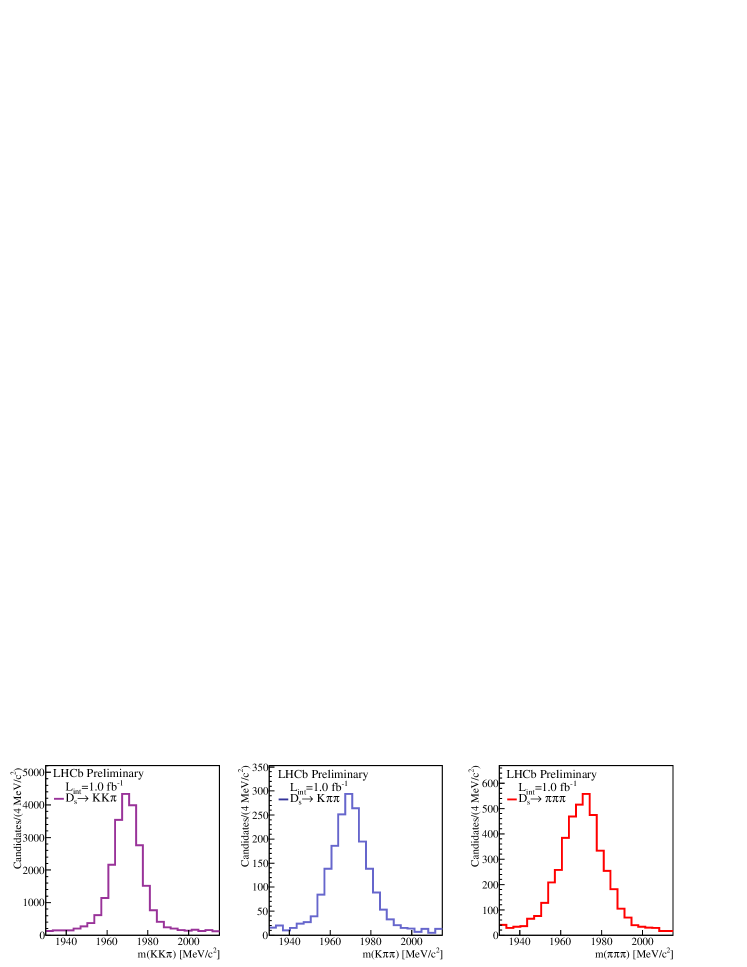
Figure 1: Invariant mass distributions for $D^{+}_{s}$ candidates in the $\kern 1.79993pt\overline{\kern-1.79993ptB}{}^{0}_{s}\rightarrow D_{s}^{+}\pi^{-}$ data sample, for (left) $K^{+}K^{-}\pi^{+}$, (middle) $K^{+}\pi^{-}\pi^{+}$, and (right) $\pi^{+}\pi^{-}\pi^{+}$ final states.

Tighter particle identification requirements are applied to the $K^{-}$ or $K^{-}\pi^{+}\pi^{-}$ recoiling from the $D^{+}_{s}$ to suppress cross-feed from the favored $\kern 1.79993pt\overline{\kern-1.79993ptB}{}^{0}_{s}\rightarrow D_{s}^{+}\pi^{-}$ and $\kern 1.79993pt\overline{\kern-1.79993ptB}{}^{0}_{s}\rightarrow D^{+}_{s}\pi^{-}\pi^{+}\pi^{-}$ decays. For the $\kern 1.79993pt\overline{\kern-1.79993ptB}{}^{0}_{s}\rightarrow D^{+}_{s}\pi^{-}\pi^{+}\pi^{-}$ and $\kern 1.79993pt\overline{\kern-1.79993ptB}{}^{0}_{s}\rightarrow D^{+}_{s}K^{-}\pi^{+}\pi^{-}$ decays, the invariant mass of the $\pi^{-}\pi^{+}\pi^{-}$ and $K^{-}\pi^{+}\pi^{-}$ systems are restricted to be below 3000 ${\mathrm{\,Me\kern-1.00006ptV\!/}c^{2}}$.

3 Analysis of $\kern 1.79993pt\overline{\kern-1.79993ptB}{}^{0}_{s}\rightarrow D_{s}^{+}\pi^{-}$ and $\kern 1.79993pt\overline{\kern-1.79993ptB}{}^{0}_{s}\rightarrow D_{s}^{+}K^{-}$

The invariant mass distributions for $\kern 1.79993pt\overline{\kern-1.79993ptB}{}^{0}_{s}\rightarrow D_{s}^{+}\pi^{-}$ and $\kern 1.79993pt\overline{\kern-1.79993ptB}{}^{0}_{s}\rightarrow D_{s}^{+}K^{-}$ are shown in Figs. 2 and 3. All three $D^{+}_{s}$ decay modes have approximately equal $B^{0}_{s}$ mass resolutions, and are summed together in these distributions. The signal shape is modeled as the sum of two Crystal Ball [14] functions, with one exponential tail on each side of the $\kern 1.79993pt\overline{\kern-1.79993ptB}{}^{0}_{s}$ signal peak. A number of specific backgrounds, due to either a missed particle (e.g. $\kern 1.79993pt\overline{\kern-1.79993ptB}{}^{0}_{s}\rightarrow D^{+}_{s}\rho^{-}$, with the $\pi^{0}$ undetected), a misidentified particle (e.g. $\kern 1.79993pt\overline{\kern-1.79993ptB}{}^{0}_{s}\rightarrow D_{s}^{+}\pi^{-}$ reconstructed as $\kern 1.79993pt\overline{\kern-1.79993ptB}{}^{0}_{s}\rightarrow D_{s}^{+}K^{-}$), or both (e.g. $\kern 1.79993pt\overline{\kern-1.79993ptB}{}^{0}_{s}\rightarrow D^{+}_{s}\rho^{-}$ reconstructed as $\kern 1.79993pt\overline{\kern-1.79993ptB}{}^{0}_{s}\rightarrow D_{s}^{+}K^{-}$) are accounted for using either data or simulation to model the shape of these backgrounds. From an unbinned extended maximum likelihood fit, $27,965\pm 395$ $\kern 1.79993pt\overline{\kern-1.79993ptB}{}^{0}_{s}\rightarrow D_{s}^{+}\pi^{-}$ and $1390\pm 98$ $\kern 1.79993pt\overline{\kern-1.79993ptB}{}^{0}_{s}\rightarrow D_{s}^{+}K^{-}$ signal events are selected.

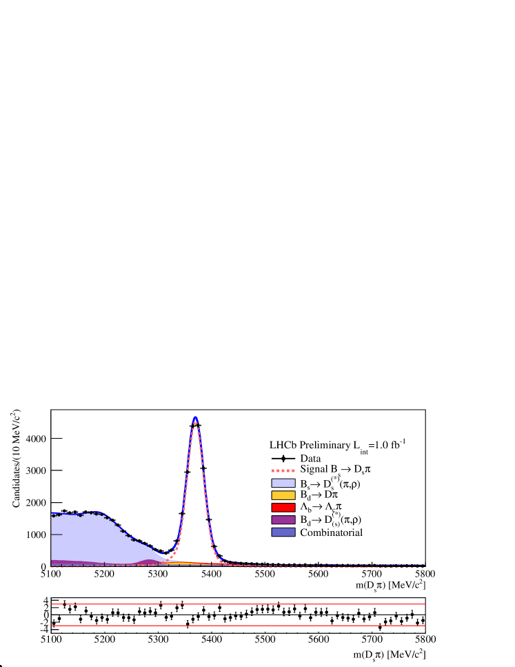
Figure 2: Invariant mass distributions $\kern 1.79993pt\overline{\kern-1.79993ptB}{}^{0}_{s}\rightarrow D_{s}^{+}\pi^{-}$ candidates. The signal component is indicated by the dashed curve, and the backgrounds are indicated by the various color-filled (shaded, in B/W) curves.

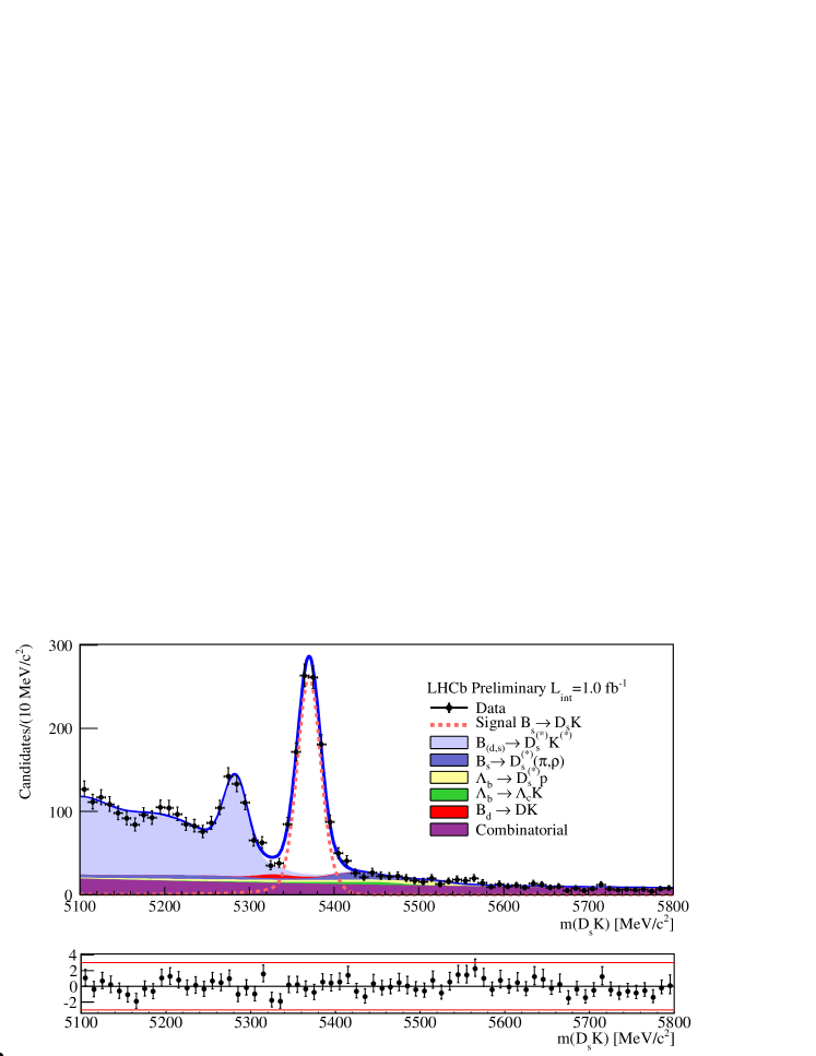
Figure 3: Invariant mass distributions $\kern 1.79993pt\overline{\kern-1.79993ptB}{}^{0}_{s}\rightarrow D_{s}^{+}K^{-}$ candidates. The signal component is indicated by the dashed curve, and the backgrounds are indicated by the various color-filled (shaded, in B/W) curves.

The CP parameters are obtained by a fit to the decay time distribution of the $\kern 1.79993pt\overline{\kern-1.79993ptB}{}^{0}_{s}\rightarrow D_{s}^{+}K^{-}$ signal candidates. Two methods have been developed. The first, referred to as sFit, uses sWeights [15] obtained from the $\kern 1.79993pt\overline{\kern-1.79993ptB}{}^{0}_{s}\rightarrow D_{s}^{+}K^{-}$ mass fit to statistically subtract the background contribution. The second method, referred to as cFit, is a conventional two-dimensional fit to the reconstructed mass and decay time. The advantage of the first method is that there is no need to model the time distribution of all the backgrounds, as they are statistically removed via the sWeights. The statistical subtraction, as presented here, uses events in the full mass fit region, and the subtraction of this background leads to a larger statistical uncertainty than if just a narrow signal region is used. For this reason, the second method is expected to give a smaller statistical uncertainty; however it requires an accurate model of the time distributions of the backgrounds that enter into the signal region. For the analysis presented here, the sFit provides the nominal result, and the cFit is used as a cross-check.

The measurement of the CP parameters in $\kern 1.79993pt\overline{\kern-1.79993ptB}{}^{0}_{s}\rightarrow D_{s}^{+}K^{-}$ requires a fit to the time-dependent decay rates. The fit accounts for (i) the acceptance versus reconstructed decay time, (ii) the decay time resolution, and (iii) the effective tagging efficiency. The functional form of the acceptance function is determined from simulated $\kern 1.79993pt\overline{\kern-1.79993ptB}{}^{0}_{s}\rightarrow D_{s}^{+}\pi^{-}$, and its parameters are determined in a fit to $\kern 1.79993pt\overline{\kern-1.79993ptB}{}^{0}_{s}\rightarrow D_{s}^{+}\pi^{-}$ data, where the $B^{0}_{s}$ lifetime and mixing frequency, $\Delta m_{s}$, are fixed to 1.51 ps and 17.69 ps^-1 [17], respectively. The average decay time resolution is about 50 fs, and is modeled by the sum of three Gaussian functions, whose parameters are determined from simulation. The Gaussian width parameters obtained from simulation are scaled up by 1.15 to account for better resolution in the simulation than in data; this factor is determined by comparing the width of the zero decay time component of prompt $D^{+}_{s}$ plus one random track in data and simulation. For the flavor tagging, only opposite side (OS) taggers are currently used. These algorithms exploit the correlation in flavor between the signal $b$ hadron at production, and the other $b$ hadron in the event (referred to as the tag-$b$). In particular, the charge of either an electron, a muon, or a kaon that does not come from any $pp$ interaction vertex (or the signal $b$), or the charge of another secondary vertex in the event, provide information on the flavor of the tag-$b$ hadron. Because $b\overline{b}$ are produced in pairs, this translates into a flavor determination of the signal $B^{0}_{s}$. The OS flavor tagging algorithm was initially tuned using simulated decays, and then re-optimized and calibrated to obtain the largest effective tagging efficiency using the self-tagging $B^{+}\rightarrow{J\mskip-3.0mu/\mskip-2.0mu\psi\mskip 2.0mu}K^{+}$ and $B^{0}\rightarrow D^{*-}\mu^{+}\nu$ decays in data. In general, the performance of the OS tagging algorithms are independent of the signal $b$-hadron decay, and have a combined effective tagging efficiency of $\epsilon D^{2}=1.90\%$ for $\kern 1.79993pt\overline{\kern-1.79993ptB}{}^{0}_{s}\rightarrow D_{s}^{+}K^{-}$. Further details of the tagging algorithms can be found in Ref [16].

In the fit to $\kern 1.79993pt\overline{\kern-1.79993ptB}{}^{0}_{s}\rightarrow D_{s}^{+}K^{-}$, the following parameters are fixed: $\Delta m_{s}=17.69$ ps^-1, $\tau_{B_{s}}=1.51$ ps and $\Delta\Gamma_{s}\equiv\Gamma_{s,L}-\Gamma_{s,H}=0.105$ ps^-1 [17]. About 60% of the $\kern 1.79993pt\overline{\kern-1.79993ptB}{}^{0}_{s}\rightarrow D_{s}^{+}K^{-}$ candidates have no flavor tag; the time-dependent decay rates for these untagged decays is given by the sum of the two expressions in Eq. LABEL:eq:decay_rates_2, and the sensitivity to $\gamma$ enters through the hyperbolic sine term. The decay time distribution of $\kern 1.79993pt\overline{\kern-1.79993ptB}{}^{0}_{s}\rightarrow D_{s}^{+}K^{-}$ signal decays and projections of the fitted are shown in Fig. 4. The projections show the four possible tagged decays, $B^{0}_{s}\rightarrow D_{s}^{\pm}K^{\mp}$ and $\kern 1.79993pt\overline{\kern-1.79993ptB}{}^{0}_{s}\rightarrow D_{s}^{\pm}K^{\mp}$, as well as the untagged time-dependent decay rates $(B^{0}_{s},\kern 1.79993pt\overline{\kern-1.79993ptB}{}^{0}_{s})\rightarrow D^{-}_{s}K^{+}$ and $(B^{0}_{s},\kern 1.79993pt\overline{\kern-1.79993ptB}{}^{0}_{s})\rightarrow D^{+}_{s}K^{-}$.

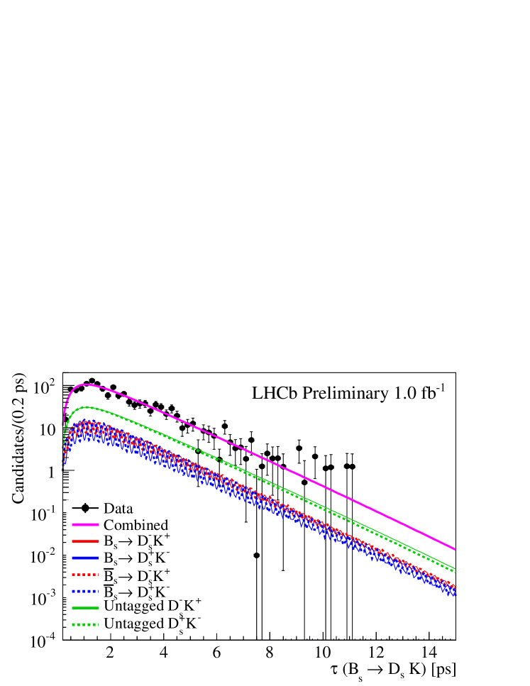
Figure 4: Distribution of reconstruct decay time for $\kern 1.79993pt\overline{\kern-1.79993ptB}{}^{0}_{s}\rightarrow D_{s}^{+}K^{-}$ signal decays (points with error bars), along with the results of the fit. Projections of the decay rates versus the decay time for the four possible flavor tagged decays, and the two untagged decays.

The fitted values for the CP parameters are

$$C =\phantom{-}1.01\pm 0.50\pm 0.23\,,$$

$$S_{f} =-1.25\pm 0.56\pm 0.24\,,$$

$$S_{\overline{f}} =\phantom{-}0.08\pm 0.68\pm 0.28\,,$$

$$D_{f} =-1.33\pm 0.60\pm 0.26\,,$$

$$D_{\overline{f}} =-0.81\pm 0.56\pm 0.26\,,$$

where the first uncertainties are statistical and the second are systematic. Several sources of systematic uncertainty have been considered. The dominant sources are due to the precision on the effective flavor tagging efficiency (0.16$\sigma_{\rm stat}$-0.23$\sigma_{\rm stat}$), variations in the parameters that are fixed in the default fits (0.15$\sigma_{\rm stat}$-0.42$\sigma_{\rm stat}$), and the correlation between the mass of specific backgrounds and their reconstructed decay time (0.08$\sigma_{\rm stat}$-0.27$\sigma_{\rm stat}$), where these uncertainties are expressed as a fraction of the statistical error. These are the first measurements of the CP parameters in $\kern 1.79993pt\overline{\kern-1.79993ptB}{}^{0}_{s}\rightarrow D_{s}^{+}K^{-}$. With additional data and analysis refinements, reduction in both the statistical and systematic uncertainties are expected.

4 First observation of $\kern 1.79993pt\overline{\kern-1.79993ptB}{}_{s}\rightarrow D^{+}_{s}K^{-}\pi^{+}\pi^{-}$ and $\kern 1.79993pt\overline{\kern-1.79993ptB}{}^{0}_{s}\rightarrow D_{s1}(2536)^{+}\pi^{-}$

The decay $\kern 1.79993pt\overline{\kern-1.79993ptB}{}^{0}_{s}\rightarrow D^{+}_{s}K^{-}\pi^{+}\pi^{-}$ can be analyzed in a similar way to $\kern 1.79993pt\overline{\kern-1.79993ptB}{}^{0}_{s}\rightarrow D_{s}^{+}K^{-}$ to measure the weak phase $\gamma$. While this decay has not yet been observed, if one uses $\kern 1.79993pt\overline{\kern-1.79993ptB}{}^{0}$ and $B^{-}$ decays as a guide, it would naively be expected that its branching fraction is 1.5-2.0 times larger than $\kern 1.79993pt\overline{\kern-1.79993ptB}{}^{0}_{s}\rightarrow D_{s}^{+}K^{-}$, making this a potentially attractive decay mode to explore. The first step in such an analysis is to firmly establish an observation of this decay and measure its branching fraction (here, relative to $\kern 1.79993pt\overline{\kern-1.79993ptB}{}^{0}_{s}\rightarrow D^{+}_{s}\pi^{-}\pi^{+}\pi^{-}$). While searching for this decay, the decay $\kern 1.79993pt\overline{\kern-1.79993ptB}{}^{0}\rightarrow D^{+}_{s}K^{-}\pi^{+}\pi^{-}$ is also observed and its branching fraction is measured relative to $\kern 1.79993pt\overline{\kern-1.79993ptB}{}^{0}_{s}\rightarrow D^{+}_{s}K^{-}\pi^{+}\pi^{-}$.

With the previously defined selections, Fig. 5 shows the invariant mass distributions for (left) $\kern 1.79993pt\overline{\kern-1.79993ptB}{}^{0}_{s}\rightarrow D^{+}_{s}\pi^{-}\pi^{+}\pi^{-}$ candidates and (right) $\kern 1.79993pt\overline{\kern-1.79993ptB}{}^{0}_{(s)}\rightarrow D^{+}_{s}K^{-}\pi^{+}\pi^{-}$ candidates. Significant $\kern 1.79993pt\overline{\kern-1.79993ptB}{}^{0}_{s}$ signals are seen in both spectra, and a $\kern 1.79993pt\overline{\kern-1.79993ptB}{}^{0}$ signal is seen in the $D^{+}_{s}K^{-}\pi^{+}\pi^{-}$ mass distribution. The main sources of background are $\kern 1.79993pt\overline{\kern-1.79993ptB}{}^{0}_{s}\rightarrow D^{*+}_{s}\pi^{-}\pi^{+}\pi^{-}$ (to $\kern 1.79993pt\overline{\kern-1.79993ptB}{}^{0}_{s}\rightarrow D^{+}_{s}\pi^{-}\pi^{+}\pi^{-}$), and $\kern 1.79993pt\overline{\kern-1.79993ptB}{}^{0}_{s}\rightarrow D^{+}_{s}\pi^{-}\pi^{+}\pi^{-}$, $\kern 1.79993pt\overline{\kern-1.79993ptB}{}^{0}_{s}\rightarrow D^{*+}_{s}\pi^{-}\pi^{+}\pi^{-}$, and $\kern 1.79993pt\overline{\kern-1.79993ptB}{}^{0}_{(s)}\rightarrow D^{*+}_{s}K^{-}\pi^{+}\pi^{-}$ (to $\kern 1.79993pt\overline{\kern-1.79993ptB}{}^{0}_{(s)}\rightarrow D^{+}_{s}K^{-}\pi^{+}\pi^{-}$). Their shapes are taken from simulation, with parameters that are allowed to vary within their uncertainties. Yields of $5683\pm 83$ $\kern 1.79993pt\overline{\kern-1.79993ptB}{}^{0}_{s}\rightarrow D^{+}_{s}\pi^{-}\pi^{+}\pi^{-}$, $216\pm 21$ $\kern 1.79993pt\overline{\kern-1.79993ptB}{}^{0}_{s}\rightarrow D^{+}_{s}K^{-}\pi^{+}\pi^{-}$ and $402\pm 33$ $\kern 1.79993pt\overline{\kern-1.79993ptB}{}^{0}\rightarrow D^{+}_{s}K^{-}\pi^{+}\pi^{-}$ are observed. After correcting for the relative efficiencies, the ratio of branching fractions are measured to be

$${{\cal{B}}(\kern 1.79993pt\overline{\kern-1.79993ptB}{}^{0}_{s}\rightarrow D^{+}_{s}K^{-}\pi^{+}\pi^{-})\over{\cal{B}}(\kern 1.79993pt\overline{\kern-1.79993ptB}{}^{0}_{s}\rightarrow D^{+}_{s}\pi^{-}\pi^{+}\pi^{-})} =(5.2\pm 0.5\pm 0.3)\times 10^{-2}$$

$${{\cal{B}}(\kern 1.79993pt\overline{\kern-1.79993ptB}{}^{0}\rightarrow D^{+}_{s}K^{-}\pi^{+}\pi^{-})\over{\cal{B}}(\kern 1.79993pt\overline{\kern-1.79993ptB}{}^{0}_{s}\rightarrow D^{+}_{s}K^{-}\pi^{+}\pi^{-})} =0.54\pm 0.07\pm 0.07,$$

where the uncertainties are statistical and systematic, respectively.

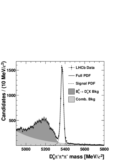
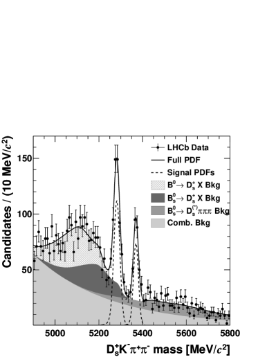
Figure 5: Invariant mass distribution for (left) $\kern 1.79993pt\overline{\kern-1.79993ptB}{}^{0}_{s}\rightarrow D^{+}_{s}\pi^{-}\pi^{+}\pi^{-}$ candidates and (right) $\kern 1.79993pt\overline{\kern-1.79993ptB}{}^{0}_{(s)}\rightarrow D^{+}_{s}K^{-}\pi^{+}\pi^{-}$ candidates. The fitted signal (dashed lines) and background shapes (shaded/hatched regions) are shown, as described in the text.

These are the first observations of these decays. Since $\kern 1.79993pt\overline{\kern-1.79993ptB}{}^{0}_{s}\rightarrow D^{+}_{s}\pi^{-}\pi^{+}\pi^{-}$ has a branching fraction that is about twice as large as $\kern 1.79993pt\overline{\kern-1.79993ptB}{}^{0}_{s}\rightarrow D_{s}^{+}\pi^{-}$, and ${\cal{B}}(\kern 1.79993pt\overline{\kern-1.79993ptB}{}^{0}_{s}\rightarrow D_{s}^{+}K^{-})\sim 0.09\times{\cal{B}}(\kern 1.79993pt\overline{\kern-1.79993ptB}{}^{0}_{s}\rightarrow D_{s}^{+}\pi^{-})$ [18], it follows that ${\cal{B}}(\kern 1.79993pt\overline{\kern-1.79993ptB}{}^{0}_{s}\rightarrow D^{+}_{s}\pi^{-}\pi^{+}\pi^{-})$ is at least as large as ${\cal{B}}(\kern 1.79993pt\overline{\kern-1.79993ptB}{}^{0}_{s}\rightarrow D_{s}^{+}\pi^{-})$, or as much as 50% larger. The ${\cal{B}}(\kern 1.79993pt\overline{\kern-1.79993ptB}{}^{0}\rightarrow D^{+}_{s}K^{-}\pi^{+}\pi^{-})$ is also sizeable, and is likely dominated by contributions where an extra $s\overline{s}$ pair is produced in addition to the weak decay (see Ref. [13] for more details).

The $\kern 1.79993pt\overline{\kern-1.79993ptB}{}^{0}_{s}\rightarrow D^{+}_{s}\pi^{-}\pi^{+}\pi^{-}$ decay has also been analyzed to search for intermediate excited $D_{sj}$ states. For $\kern 1.79993pt\overline{\kern-1.79993ptB}{}^{0}_{s}\rightarrow D^{+}_{s}\pi^{-}\pi^{+}\pi^{-}$ candidates within 40 ${\mathrm{\,Me\kern-1.00006ptV\!/}c^{2}}$ of the $\kern 1.79993pt\overline{\kern-1.79993ptB}{}^{0}_{s}$ signal peak, the mass difference, $\Delta M\equiv M(D^{+}_{s}\pi^{-}\pi^{+})-M(D^{+}_{s})$ is computed for both $\pi^{-}\pi^{+}$ mass combinations. The resulting mass difference spectrum is shown in Fig. 6. The signal is fit with a Breit-Wigner convolved with a Gaussian resolution function whose width is fixed to the expected $\Delta M$ resolution. A signal of $20.0\pm 5.1$ events is observed with a $\Delta M$ value and width consistent with the $D_{s1}(2536)^{+}$ state. Applying corrections for the relative efficiency, the ratio of branching fractions is measured to be

$${{\cal{B}}(\kern 1.79993pt\overline{\kern-1.79993ptB}{}^{0}_{s}\rightarrow D_{s1}(2536)^{+}\pi^{-},~{}D_{s1}^{+}\rightarrow D^{+}_{s}\pi^{-}\pi^{+})\over{\cal{B}}(\kern 1.79993pt\overline{\kern-1.79993ptB}{}^{0}_{s}\rightarrow D^{+}_{s}\pi^{-}\pi^{+}\pi^{-})}=(4.0\pm 1.0\pm 0.4)\times 10^{-3}.$$

The excess of events is 5.9 standard deviations over the expected background, thus establishing the first observation of this decay.

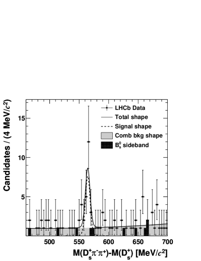
Figure 6: Distribution of the difference in invariant mass, $M(D^{+}_{s}\pi^{-}\pi^{+})-M(D^{+}_{s})$, using $\kern 1.79993pt\overline{\kern-1.79993ptB}{}^{0}_{s}\rightarrow D^{+}_{s}\pi^{-}\pi^{+}\pi^{-}$ candidates within 40 ${\mathrm{\,Me\kern-1.00006ptV\!/}c^{2}}$ of the known $B^{0}_{s}$ mass (points) and in the upper $B^{0}_{s}$ mass sidebands (filled histogram). The fit to the distribution is shown, as described in the text.

5 Summary

First measurements of the CP observables in the $\kern 1.79993pt\overline{\kern-1.79993ptB}{}^{0}_{s}\rightarrow D_{s}^{+}K^{-}$ decay have been reported. With the larger data sample recorded in 2012, and the larger data set anticipated in the future, this decay will contribute significantly to the determination of the weak phase $\gamma$. First observations of the $\kern 1.79993pt\overline{\kern-1.79993ptB}{}^{0}_{s}\rightarrow D^{+}_{s}K^{-}\pi^{+}\pi^{-}$ and $\kern 1.79993pt\overline{\kern-1.79993ptB}{}^{0}\rightarrow D^{+}_{s}K^{-}\pi^{+}\pi^{-}$ are also reported. The former can be used in a similar way to $\kern 1.79993pt\overline{\kern-1.79993ptB}{}^{0}_{s}\rightarrow D_{s}^{+}K^{-}$ to extract $\gamma$. After including $D^{+}_{s}\rightarrow\pi^{+}\pi^{-}\pi^{+}$ and $D^{+}_{s}\rightarrow K^{-}\pi^{+}\pi^{-}$ decays, and reoptimizing the selection for $\kern 1.79993pt\overline{\kern-1.79993ptB}{}^{0}_{s}\rightarrow D^{+}_{s}K^{-}\pi^{+}\pi^{-}$ only, the yield in this mode more than doubles with a comparable signal-to-background. The yield in this mode is therefore expected to have about 35-40% of that obtained in $\kern 1.79993pt\overline{\kern-1.79993ptB}{}^{0}_{s}\rightarrow D_{s}^{+}K^{-}$. The $\kern 1.79993pt\overline{\kern-1.79993ptB}{}^{0}_{s}\rightarrow D_{s1}(2536)^{+}\pi^{-}$ decay is also observed for the first time, and its branching fraction relative to $\kern 1.79993pt\overline{\kern-1.79993ptB}{}^{0}_{s}\rightarrow D^{+}_{s}\pi^{-}\pi^{+}\pi^{-}$ is presented.

References

- [1] N. Cabibbo, Phys. Rev. Lett. 10, 531 (1963).
- [2] M. Kobayashi and T. Maskawa, Prog. Theor. Phys. 49, 652 (1973).
- [3] See talks by G. Eigen and D. Derkach in these proceedings; Also, see S. Descotes-Genon et al. (CKMFitter collaboration), Proceedings Supplements, Capri, Italy, July 11-13, 2012, to be published in Nucl. Phys. B. Updated results and plots available at: http://ckmfitter.in2p3.fr; Also, M. Bona (UTFit collaboration), Proceedings Supplements, Capri, Italy, July 11-13, 2012, to be published in Nucl. Phys. B, with updated results at http://www.utfit.org/UTFit.
- [4] L. Wolfenstein, Phys. Rev. Lett. 51, 1945 (1983).
- [5] See contributions by S. Malde and M. John, these proceedings.
- [6] D. Atwood, G. Eilam, M. Gronau, and A. Soni, Phys. Lett. B341, 372 (1995).
- [7] M. Gronau and D. London, Phys. Lett. B253, 483 (1991); M. Gronau and D. Wyler, Phys. Lett. B265, 172 (1991).
- [8] A. Giri, Y. Grossman, A. Soffer, and J. Zupan, Phys. Rev. D68, 054018 (2003).
- [9] R. Aleksan, I. Dunietz and B. Kayser, Z. Phys. C54, 653 (1992).
- [10] R. Fleischer, Nucl. Phys. B671, 459 (2003).
- [11] K. De Bruyn, R. Fleischer, R. Knegjens, M. Merk, M. Schiller and N. Tuning, Nucl. Phys. B868, 351 (2012).
- [12] LHCb collaboration, LHCb-CONF-2012-029.
- [13] R. Aaij (LHCb collaboration), LHCb-PAPER-2012-033, arXiv:1211.1541, submitted to Phys. Rev. D.
- [14] T. Skwarnicki, PhD thesis, Institute of Nuclear Physics, Krakow, 1986, DESY-F31-86-02.
- [15] M. Pivk and F. R. Le Diberder, Nucl. Instrum. Meth. A555, 356 (2005).
- [16] R. Aaij et. al. (LHCb Collaboration), Eur. Phys. J. C72, 2022 (2012); LHCb-CONF-2012-026; Also see contribution by J. Wishahi in these proceedings.
- [17] Heavy Flavor Averaging Group, D. Asner et al., Averages of b-hadron, chadron, and tau-lepton Properties, arXiv:1010.1589, Online updates available at http://www.slac.stanford.edu/xorg/hfag/.
- [18] Particle Data Group, J. Beringer et al., Phys. Rev. D86, 010001 (2012).