Stability of R𝑅R parity in supersymmetric models extended By U(1)BL𝑈subscript1𝐵𝐿U(1)_{B-L}

J. E. Camargo-Molina jose.camargo@physik.uni-wuerzburg.de    B. O’Leary ben.oleary@physik.uni-wuerzburg.de    W. Porod porod@physik.uni-wuerzburg.de Institut für Theoretische Physik und Astronomie, Universität Würzburg
Am Hubland, 97074 Wuerzburg
   F. Staub fnstaub@th.physik.uni-bonn.de Bethe Center for Theoretical Physics & Physikalisches Institut der Universität Bonn,
53115 Bonn, Germany
Abstract

We perform a study of the stability of R𝑅R-parity-conserving vacua of a constrained version of the minimal supersymmetric model with a gauged U(1)BL𝑈subscript1𝐵𝐿U(1)_{B-L} which can conserve R𝑅R-parity, using homotopy continuation to find all the extrema of the tree-level potential, for which we also calculated the one-loop corrections. While we find that a majority of the points in the parameter space preserve R𝑅R-parity, we find that a significant portion of points which naïvely have phenomenologically acceptable vacua which conserve R𝑅R-parity actually have deeper vacua which break R𝑅R-parity through sneutrino VEVs. We investigate under what conditions the deeper R𝑅R-parity-violating vacua appear. We find that while previous exploratory work was broadly correct in some of its qualitative conclusions, we disagree in detail.

supersymmetry, R-parity violation, vacuum stability, extended gauge sector
pacs:
??, ??, ??
preprint: Bonn-TH-2012-033

I Introduction

With the discovery of a resonance at 126 GeV at the LHC :2012gk ; :2012gu , the interpretation that it is the Higgs boson of the standard model (SM) raises the issue of the stability of the SM vacuum Isidori:2001bm ; Ellis:2009tp ; EliasMiro:2011aa ; Bezrukov:2012sa ; Degrassi:2012ry . Since there is only one field in the SM that can possibly have a non-zero vacuum expectation value (VEV) (assuming Lorentz invariance), finding the minima of the potential energy is straightforward, though of course evaluating it to the accuracy required is quite involved EliasMiro:2011aa ; Bezrukov:2012sa ; Degrassi:2012ry .

Many extensions of the SM introduce extra scalar fields, and thus could in principle have many more VEVs. In particular, the minimal supersymmetric extension of the SM (MSSM) not only introduces complex scalar partners for each SM fermion, it also introduces a second Higgs SU(2)L𝑆𝑈subscript2𝐿SU(2)_{L} doublet. Even only allowing for the neutral components of the Higgs doublets to gain non-zero VEVs, the vacuum structure is non-trivial. Fortunately, as a particular case of a two-Higgs-doublet model, there is a proof that at tree level, there are at most two minima that conserve electric charge Ivanov:2006yq , and there are analytic formulae to determine which vacuum has a lower energy at tree level Barroso:2012mj .

However, the possibility of VEVs for the scalar partners of the SM fermions, the sfermions, is a troubling prospect, as all but the sneutrinos are charged under SU(3)c𝑆𝑈subscript3𝑐SU(3)_{c} and/or U(1)em𝑈subscript1𝑒𝑚U(1)_{em}, and thus any VEVs for these scalars are ruled out by these being good symmetries of the vacuum. Unfortunately, the potential as a function of several scalar fields is so complicated that even at tree level, finding the global minimum is highly non-trivial, in general Claudson:1983et ; Drees:1985ie ; Gunion:1987qv ; Kuchimanchi:1993jg ; Casas:1995pd . The only tractable approaches thus far have been to investigate the “most dangerous” possibilities of stop or stau VEVs  Gunion:1987qv ; Kitahara:2012pb ; Carena:2012mw .

Sneutrino VEVs, on the other hand, are not necessarily a problem111For example, in the case of bilinear R𝑅R-parity violation, the sneutrino VEVs have to be small to explain neutrino data implying that in this model essentially the conclusions concerning the minima of the potential can be taken over from the MSSM Hirsch:2004hr .. Of course, they would break R𝑅R-parity, leading to mixings between SM and SUSY particles carrying the same spin and SU(3)c×U(1)em𝑆𝑈subscript3𝑐𝑈subscript1𝑒𝑚SU(3)_{c}\times U(1)_{em} quantum numbers, see e.gHirsch:2000ef and refs. therein. However, in the absence of baryon-number-violating trilinear couplings in the superpotential, proton decay would still be perturbatively forbidden. If R𝑅R-parity is conserved, the lightest supersymmetric partner (LSP), if uncharged under SU(3)c𝑆𝑈subscript3𝑐SU(3)_{c} and U(1)em𝑈subscript1𝑒𝑚U(1)_{em}, could be a perturbatively stable dark matter candidate Ellis:1983ew ; Ellis:2003cw . If R𝑅R-parity is not conserved, the LSP is not absolutely stable, but, depending on the size of the sneutrino VEVs, a small amount of R𝑅R-parity violation still allows for a metastable LSP to make up the observed dark matter. However, even if the neutralino is not sufficiently long-lived, another particle like the gravitino Borgani:1996ag ; Takayama:2000uz ; Hirsch:2005ag ; Covi:2008jy ; Steffen:2008qp or the axion Rajagopal:1990yx ; Goto:1991gq ; Steffen:2008qp could be long-lived enough to serve as dark matter.

The conservation of baryon number B𝐵B and of lepton number L𝐿L is only accidental in the SM, and this conservation through the imposition of R𝑅R-parity may appear to be rather ad hoc in the MSSM, since the only difference between a lepton SU(2)L𝑆𝑈subscript2𝐿SU(2)_{L} doublet and the Higgs SU(2)L𝑆𝑈subscript2𝐿SU(2)_{L} doublet responsible for mass for the down-type quarks Hdsubscript𝐻𝑑H_{d} is that Hdsubscript𝐻𝑑H_{d} is assigned L=0𝐿0L=0 instead of 111. Still, noting that R𝑅R-parity is defined as (1)(3B+L2s)=(1)(3(BL)2s)superscript13𝐵𝐿2𝑠superscript13𝐵𝐿2𝑠(-1)^{(3B+L-2s)}=(-1)^{(3(B-L)-2s)} if lepton number is integer or half-integer for every field, one may consider a symmetry based on BL𝐵𝐿B-L as a motivated extension.

Adding U(1)BL𝑈subscript1𝐵𝐿U(1)_{B-L} as an extension to the SM Khalil:2006yi ; Emam:2007dy ; Basso:2008iv ; Basso:2010yz ; Basso:2010si or the MSSM Khalil:2007dr ; Barger:2008wn ; FileviezPerez:2010ek has been considered quite a lot in the literature, as in addition to motivating R𝑅R-parity, it leads to a rich phenomenology, and, in some models, naturally leads to type I see-saw mechanisms for neutrino masses.

The most minimal of such extensions of the MSSM requires superfields with right-handed neutrinos as fermionic components to cancel gauge anomalies, and their scalar components provide the VEVs necessary to break U(1)BL𝑈subscript1𝐵𝐿U(1)_{B-L} as required by phenomenology. Already such a model has eight complex scalar fields that in principle could have non-zero VEVs without breaking SU(3)c𝑆𝑈subscript3𝑐SU(3)_{c} or U(1)em𝑈subscript1𝑒𝑚U(1)_{em}, with many possible minima.

Conserved R𝑅R-parity is still attractive from a phenomenological point of view, since there are tight limits on many R𝑅R-parity-violating parameters Dreiner:2006gu ; Dreiner:2010ye ; Dreiner:2012mx . One can extend the neutral sector with further superfields with VEVs which break U(1)BL𝑈subscript1𝐵𝐿U(1)_{B-L} without breaking R𝑅R-parity Khalil:2007dr ; FileviezPerez:2010ek . However, given the complicated structure of the potential, it is prudent to be concerned about whether such extensions really do conserve R𝑅R-parity at their global minima over relevant parameter ranges.

In the following sections, we investigate how stable R𝑅R-parity-conserving vacua are in such a minimal U(1)BL𝑈subscript1𝐵𝐿U(1)_{B-L}-gauged extension of the MSSM. In sec. II, we define the model. In sec. III, we describe how we approach the difficult problem of minimizing such a complicated potential, including going to the full one-loop potential, since it is well-known that there can be rather large corrections in the Higgs sector of the MSSM Okada:1990vk ; Okada:1990gg ; Ellis:1990nz ; Haber:1990aw ; Ellis:1991zd ; Chankowski:1991md ; Brignole:1992uf ; Dabelstein:1994hb ; Hempfling:1993qq ; Haber:1996fp ; Heinemeyer:1998jw ; Heinemeyer:1998kz ; Heinemeyer:1998np ; Zhang:1998bm ; Espinosa:1999zm ; Espinosa:2001mm ; Degrassi:2001yf ; Brignole:2002bz ; Brignole:2001jy ; Degrassi:2002fi ; Martin:2002wn ; Allanach:2004rh ; Harlander:2008ju ; Kant:2010tf . In sec. IV, we present the results of two scans over phenomenologically interesting regions of the parameter space, and in sec. IV.1, we compare our results to previous investigations in the literature. Finally, we sum up in sec. V.

II The model

II.1 Particle content and superpotential

There are several ways to extend the MSSM by U(1)BL𝑈subscript1𝐵𝐿U(1)_{B-L}. Here we choose the minimal extension which allows for a spontaneously broken U(1)BL𝑈subscript1𝐵𝐿U(1)_{B-L} without necessarily breaking R𝑅R-parity. This requires the addition of two SM gauge-singlet chiral superfields carrying BL𝐵𝐿B-L which may develop VEVs, as well as the addition of three generations of superfields containing right-handed neutrinos. We refer to this model as the BLSSM.

The BLSSM appears to be a relatively straightforward extension of the MSSM, yet it has a rich phenomenology, with a Zsuperscript𝑍Z^{\prime} boson (with prospects for the LHC discussed in Krauss:2012ku ), Majorana neutrinos with see-saw masses, several qualitatively new dark matter candidates with respect to the MSSM Basso:2012gz , and a rich Higgs boson sector Basso:2012tr . It also has many interesting technicalities Fonseca:2011vn , which are fully explained in OLeary:2011yq .

However, all the above works assume that R𝑅R-parity is conserved. Indeed, the model was constructed as the minimal extension of the MSSM that includes U(1)BL𝑈subscript1𝐵𝐿U(1)_{B-L} as an extra gauge symmetry, while allowing it to break spontaneously without necessarily violating the conservation of R𝑅R-parity. As mentioned in the introduction, VEVs for the scalar partners of the right-handed neutrinos could break U(1)BL𝑈subscript1𝐵𝐿U(1)_{B-L} at the cost of losing R𝑅R-parity, and aspects of the LHC phenomenology in the case of broken R𝑅R-parity are discussed in FileviezPerez:2011kd ; FileviezPerez:2012mj . The purpose of this work is to investigate how robustly R𝑅R-parity is conserved for parameters of phenomenological interest.

While we refer the reader to Ref. OLeary:2011yq for a full description of the BLSSM and its implementation in SARAH Staub:2008uz ; Staub:2009bi ; Staub:2010jh ; Staub:2012pb and SPheno Porod:2003um ; Porod:2011nf , for reference we recap the gauge symmetries and particle content of the model here.

The model consists of three generations of matter particles including right-handed neutrinos which can, for example, be embedded in SO(10)𝑆𝑂10SO(10) 16-plets. For convenience, we refer to their scalar components as R-sneutrinos. Moreover, below the GUT scale the usual MSSM Higgs doublets are present, as well as two fields η𝜂\eta and η¯¯𝜂\bar{\eta} responsible for the breaking of the U(1)BL𝑈subscript1𝐵𝐿U(1)_{B-L}. Furthermore, η𝜂\eta is responsible for generating a Majorana mass term for the right-handed neutrinos and thus we interpret the BL𝐵𝐿B-L charge of this field as its lepton number, and likewise for η¯¯𝜂\bar{\eta}, and call these fields bileptons since they carry twice the lepton number of (anti-)neutrinos. We summarize the quantum numbers of the chiral superfields with respect to the model’s gauge group U(1)Y×SU(2)L×SU(3)C×U(1)BL𝑈subscript1𝑌𝑆𝑈subscript2𝐿𝑆𝑈subscript3𝐶𝑈subscript1𝐵𝐿U(1)_{Y}\times SU(2)_{L}\times SU(3)_{C}\times{U(1)_{B-L}} in Tab. 1.

Superfield Spin 0 Spin 1212\frac{1}{2} Generations U(1)YSU(2)LSU(3)CU(1)BLtensor-producttensor-producttensor-product𝑈subscript1𝑌𝑆𝑈subscript2𝐿𝑆𝑈subscript3𝐶𝑈subscript1𝐵𝐿U(1)_{Y}\otimes\,SU(2)_{L}\otimes\,SU(3)_{C}\otimes\,{U(1)_{B-L}}
Q^^𝑄\hat{Q} Q~~𝑄\tilde{Q} Q𝑄Q 3 (16,𝟐,𝟑,16)162316(\frac{1}{6},{\bf 2},{\bf 3},\frac{1}{6})
d^csuperscript^𝑑𝑐\hat{d}^{c} d~csuperscript~𝑑𝑐\tilde{d}^{c} dcsuperscript𝑑𝑐d^{c} 3 (13,𝟏,𝟑¯,16)131¯316(\frac{1}{3},{\bf 1},{\bf\overline{3}},-\frac{1}{6})
u^csuperscript^𝑢𝑐\hat{u}^{c} u~csuperscript~𝑢𝑐\tilde{u}^{c} ucsuperscript𝑢𝑐u^{c} 3 (23,𝟏,𝟑¯,16)231¯316(-\frac{2}{3},{\bf 1},{\bf\overline{3}},-\frac{1}{6})
L^^𝐿\hat{L} L~~𝐿\tilde{L} L𝐿L 3 (12,𝟐,𝟏,12)122112(-\frac{1}{2},{\bf 2},{\bf 1},-\frac{1}{2})
e^csuperscript^𝑒𝑐\hat{e}^{c} e~csuperscript~𝑒𝑐\tilde{e}^{c} ecsuperscript𝑒𝑐e^{c} 3 (1,𝟏,𝟏,12)11112(1,{\bf 1},{\bf 1},\frac{1}{2})
ν^csuperscript^𝜈𝑐\hat{\nu}^{c} ν~csuperscript~𝜈𝑐\tilde{\nu}^{c} νcsuperscript𝜈𝑐\nu^{c} 3 (0,𝟏,𝟏,12)01112(0,{\bf 1},{\bf 1},\frac{1}{2})
H^dsubscript^𝐻𝑑\hat{H}_{d} Hdsubscript𝐻𝑑H_{d} H~dsubscript~𝐻𝑑\tilde{H}_{d} 1 (12,𝟐,𝟏,0)12210(-\frac{1}{2},{\bf 2},{\bf 1},0)
H^usubscript^𝐻𝑢\hat{H}_{u} Husubscript𝐻𝑢H_{u} H~usubscript~𝐻𝑢\tilde{H}_{u} 1 (12,𝟐,𝟏,0)12210(\frac{1}{2},{\bf 2},{\bf 1},0)
η^^𝜂\hat{\eta} η𝜂\eta η~~𝜂\tilde{\eta} 1 (0,𝟏,𝟏,1)0111(0,{\bf 1},{\bf 1},-1)
η¯^^¯𝜂\hat{\bar{\eta}} η¯¯𝜂\bar{\eta} η¯~~¯𝜂\tilde{\bar{\eta}} 1 (0,𝟏,𝟏,1)0111(0,{\bf 1},{\bf 1},1)
Table 1: Chiral superfields and their quantum numbers.

The superpotential is given by

W=𝑊absent\displaystyle W= Yuiju^icQ^jH^uYdijd^icQ^jH^dYeije^icL^jH^d+μH^uH^dsubscriptsuperscript𝑌𝑖𝑗𝑢subscriptsuperscript^𝑢𝑐𝑖subscript^𝑄𝑗subscript^𝐻𝑢superscriptsubscript𝑌𝑑𝑖𝑗subscriptsuperscript^𝑑𝑐𝑖subscript^𝑄𝑗subscript^𝐻𝑑subscriptsuperscript𝑌𝑖𝑗𝑒subscriptsuperscript^𝑒𝑐𝑖subscript^𝐿𝑗subscript^𝐻𝑑𝜇subscript^𝐻𝑢subscript^𝐻𝑑\displaystyle\,Y^{ij}_{u}\,\hat{u}^{c}_{i}\,\hat{Q}_{j}\,\hat{H}_{u}\,-Y_{d}^{ij}\,\hat{d}^{c}_{i}\,\hat{Q}_{j}\,\hat{H}_{d}\,-Y^{ij}_{e}\,\hat{e}^{c}_{i}\,\hat{L}_{j}\,\hat{H}_{d}\,+\mu\,\hat{H}_{u}\,\hat{H}_{d}\,
+Yνijν^icL^jH^uμη^η¯^+Yxijν^icη^ν^jc,subscriptsuperscript𝑌𝑖𝑗𝜈subscriptsuperscript^𝜈𝑐𝑖subscript^𝐿𝑗subscript^𝐻𝑢superscript𝜇^𝜂^¯𝜂subscriptsuperscript𝑌𝑖𝑗𝑥subscriptsuperscript^𝜈𝑐𝑖^𝜂subscriptsuperscript^𝜈𝑐𝑗\displaystyle\,\,+Y^{ij}_{\nu}\,\hat{\nu}^{c}_{i}\,\hat{L}_{j}\,\hat{H}_{u}\,-\mu^{\prime}\,\hat{\eta}\,\hat{\bar{\eta}}\,+Y^{ij}_{x}\,\hat{\nu}^{c}_{i}\,\hat{\eta}\,\hat{\nu}^{c}_{j}\,, (1)

and we have the additional soft SUSY-breaking terms:

SB=subscript𝑆𝐵absent\displaystyle\mathscr{L}_{SB}= MSSMmη2|η|2mη¯2|η¯|2mνc,ij2(ν~ic)ν~jcsubscript𝑀𝑆𝑆𝑀superscriptsubscript𝑚𝜂2superscript𝜂2superscriptsubscript𝑚¯𝜂2superscript¯𝜂2superscriptsubscript𝑚superscript𝜈𝑐𝑖𝑗2superscriptsuperscriptsubscript~𝜈𝑖𝑐superscriptsubscript~𝜈𝑗𝑐\displaystyle\mathscr{L}_{MSSM}-m_{\eta}^{2}|\eta|^{2}-m_{\bar{\eta}}^{2}|\bar{\eta}|^{2}-{m_{\nu^{c},ij}^{2}}(\tilde{\nu}_{i}^{c})^{*}\tilde{\nu}_{j}^{c}
+(TνijHuν~icL~j+Txijην~icν~jcλB~λB~MBB12λB~λB~MBηη¯Bμ+c.c),\displaystyle+\left(T^{ij}_{\nu}H_{u}\tilde{\nu}_{i}^{c}\tilde{L}_{j}+T^{ij}_{x}\eta\tilde{\nu}_{i}^{c}\tilde{\nu}_{j}^{c}-\lambda_{\tilde{B}}\lambda_{\tilde{B}^{\prime}}{M}_{BB^{\prime}}-\frac{1}{2}\lambda_{\tilde{B}^{\prime}}\lambda_{\tilde{B}^{\prime}}{M}_{B^{\prime}}-\eta\bar{\eta}B_{\mu^{\prime}}+c.c\right), (2)

with i,j𝑖𝑗i,j being the generation indices. Without loss of generality one can take Bμsubscript𝐵𝜇B_{\mu} and Bμsubscript𝐵superscript𝜇B_{\mu^{\prime}} to be real. The extended gauge group breaks to SU(3)CU(1)emtensor-product𝑆𝑈subscript3𝐶𝑈subscript1𝑒𝑚SU(3)_{C}\otimes U(1)_{em} as the Higgs fields and bileptons receive vacuum expectation values (VEVs):

Hd0=superscriptsubscript𝐻𝑑0absent\displaystyle H_{d}^{0}= 12(vd+σd+iϕd),Hu0=12(vu+σu+iϕu),12subscript𝑣𝑑subscript𝜎𝑑𝑖subscriptitalic-ϕ𝑑superscriptsubscript𝐻𝑢012subscript𝑣𝑢subscript𝜎𝑢𝑖subscriptitalic-ϕ𝑢\displaystyle\,\frac{1}{\sqrt{2}}\left(v_{d}+\sigma_{d}+i\phi_{d}\right),\hskip 28.45274ptH_{u}^{0}=\,\frac{1}{\sqrt{2}}\left(v_{u}+\sigma_{u}+i\phi_{u}\right), (3)
η=𝜂absent\displaystyle\eta= 12(vη+ση+iϕη),η¯=12(vη¯+ση¯+iϕη¯).12subscript𝑣𝜂subscript𝜎𝜂𝑖subscriptitalic-ϕ𝜂¯𝜂12subscript𝑣¯𝜂subscript𝜎¯𝜂𝑖subscriptitalic-ϕ¯𝜂\displaystyle\,\frac{1}{\sqrt{2}}\left(v_{\eta}+\sigma_{\eta}+i\phi_{\eta}\right),\hskip 28.45274pt\bar{\eta}=\,\frac{1}{\sqrt{2}}\left(v_{\bar{\eta}}+\sigma_{\bar{\eta}}+i\phi_{\bar{\eta}}\right). (4)

We define tanβ=vη/vη¯superscript𝛽subscript𝑣𝜂subscript𝑣¯𝜂\tan\beta^{\prime}=v_{\eta}/v_{\bar{\eta}} in analogy to the ratio of the MSSM VEVs (tanβ=vu/vd𝛽subscript𝑣𝑢subscript𝑣𝑑\tan\beta=v_{u}/v_{d}). For certain parameter combinations a spontaneous breakdown of R𝑅R-parity can occur as also some or all sneutrinos can obtain non-vanishing VEVs FileviezPerez:2010ek . We denote the VEVs for the sneutrinos of the SU(2)L𝑆𝑈subscript2𝐿SU(2)_{L} doublets L~isubscript~𝐿𝑖\tilde{L}_{i} by vL,isubscript𝑣𝐿𝑖v_{L,i} and those of the SU(2)L𝑆𝑈subscript2𝐿SU(2)_{L} singlet sneutrinos ν~icsubscriptsuperscript~𝜈𝑐𝑖\tilde{\nu}^{c}_{i} by vR,isubscript𝑣𝑅𝑖v_{R,i}, with i=1,2,3𝑖123i=1,2,3.

II.2 Constrained model

We will consider in the following a scenario motivated by minimal supergravity assuming a GUT unification of all soft SUSY-breaking scalar mass parameters as well as a unification of all gaugino mass parameters:

m02=subscriptsuperscript𝑚20absent\displaystyle m^{2}_{0}= mHd2=mHu2=mη2=mη¯2,subscriptsuperscript𝑚2subscript𝐻𝑑subscriptsuperscript𝑚2subscript𝐻𝑢subscriptsuperscript𝑚2𝜂subscriptsuperscript𝑚2¯𝜂\displaystyle m^{2}_{H_{d}}=m^{2}_{H_{u}}=m^{2}_{\eta}=m^{2}_{\bar{\eta}}, (5)
m02𝟏=subscriptsuperscript𝑚201absent\displaystyle m^{2}_{0}\mathbf{1}= mD2=mU2=mQ2=mE2=mL2=mν~c2,superscriptsubscript𝑚𝐷2superscriptsubscript𝑚𝑈2superscriptsubscript𝑚𝑄2superscriptsubscript𝑚𝐸2superscriptsubscript𝑚𝐿2superscriptsubscript𝑚superscript~𝜈𝑐2\displaystyle m_{D}^{2}=m_{U}^{2}=m_{Q}^{2}=m_{E}^{2}=m_{L}^{2}={m_{{\tilde{\nu}}^{c}}^{2}}, (6)
M1/2=subscript𝑀12absent\displaystyle M_{1/2}= M1=M2=M3=MB~.subscript𝑀1subscript𝑀2subscript𝑀3subscript𝑀superscript~𝐵\displaystyle M_{1}=M_{2}=M_{3}=M_{\tilde{B}^{\prime}}. (7)

Also, for the trilinear soft SUSY-breaking couplings, we assume the ordinary mSUGRA-inspired conditions

Ti=A0Yi,i=e,d,u,x,ν.formulae-sequencesubscript𝑇𝑖subscript𝐴0subscript𝑌𝑖𝑖𝑒𝑑𝑢𝑥𝜈\displaystyle T_{i}=A_{0}Y_{i},\hskip 28.45274pti=e,d,u,x,\nu\thickspace. (8)

Furthermore, we assume that there are no off-diagonal gauge couplings or off-diagonal gaugino mass parameters present at the GUT scale, motivated by the possibility that the two Abelian groups are a remnant of a larger product group which gets broken at the GUT scale, as discussed in OLeary:2011yq , to which we refer the reader for details of the gauge coupling structure.

In addition, we consider the mass of the Zsuperscript𝑍Z^{\prime} and tanβsuperscript𝛽\tan\beta^{\prime} as inputs and use the following set of free parameters:

m0,M1/2,A0,tanβ,tanβ,sign(μ),sign(μ),mZ,YxandYν.subscript𝑚0subscript𝑀12subscript𝐴0𝛽superscript𝛽sign𝜇signsuperscript𝜇subscript𝑚superscript𝑍subscript𝑌𝑥andsubscript𝑌𝜈\displaystyle m_{0},\thickspace M_{1/2},\thickspace A_{0},\thickspace\tan\beta,\thickspace\tan\beta^{\prime},\thickspace\text{sign}(\mu),\thickspace\text{sign}(\mu^{\prime}),\thickspace{m_{Z^{\prime}}},\thickspace Y_{x}\thickspace\mbox{and}\thickspace Y_{\nu}. (9)

Yνsubscript𝑌𝜈Y_{\nu} is constrained by neutrino data and must therefore be very small in comparison to the other couplings in this model, as required by the embedded TeV-scale type-I seesaw mechanism, so we take Yνij=105δijsuperscriptsubscript𝑌𝜈𝑖𝑗superscript105superscript𝛿𝑖𝑗Y_{\nu}^{ij}=10^{-5}{\delta}^{ij} as its precise structure does not affect any of our conclusions. Yxsubscript𝑌𝑥Y_{x} can always be taken diagonal and thus effectively we have 9 free parameters and 2 signs. We denote this constrained version of the BLSSM as the CBLSSM.

III Minimizing the potential

The primary question that we wish to answer is: within the CBLSSM, what portion of the parameter points which have a phenomenologically acceptable, R𝑅R-parity-conserving local minimum of the potential turn out to have a global minimum with different VEVs, and are there any patterns in the parameters of such points? By “phenomenologically acceptable”, we restrict ourselves to parameter points which have a local minimum with the expectation values of the Higgs doublets leading to the correct values for mWsubscript𝑚𝑊m_{W} and mZsubscript𝑚𝑍m_{Z}, there are no tachyons, and no charged or colored scalar has a VEV. Hence any minima that are “phenomenologically acceptable” and R𝑅R-parity-conserving have expectation values for the Higgs doublet fields Hd,Husubscript𝐻𝑑subscript𝐻𝑢H_{d},H_{u} and the bilepton fields η,η¯𝜂¯𝜂\eta,\bar{\eta}, and no other field has a non-zero expectation value.

Our method to address this question was as follows: we performed a random scan over a range of input parameters, constrained to having phenomenologically acceptable, R𝑅R-parity-conserving local minima at expectation values for the Higgs doublet and bilepton fields given as input; we then found all the extrema of the tree-level potential for each parameter point allowing non-zero sneutrino VEVs; we evaluated the loop-corrected potential at these points (ensuring that the corrections did not move the minima significantly) and selected the deepest, and thus can say if the minimum chosen as input was not the global minimum.

III.1 Generation of parameter points

The package SARAH was used to create a SPheno executable specific to the CBLSSM, which was used with the SSP package Staub:2011dp to perform random scans over two different parameter regions. The first scan, which we refer to as the “democratic” scan, took random values for each diagonal entry of the R-sneutrino – bilepton Yukawa coupling Yxsubscript𝑌𝑥Y_{x} independently over its range. The other, which we refer to as the “hierarchical” scan, kept the (1,1)11(1,1) and (2,2)22(2,2) entries as 103superscript10310^{-3} and 102superscript10210^{-2} respectively. The hierarchical scan was motivated by the hierarchy of the quark and charged lepton Yukawa couplings, but is not favored for any other reason. The ranges of the CBLSSM parameters for each scan are shown in Tab. 2.

The mass parameter ranges were chosen to be consistent with non-observation of sparticles at the LEP and LHC experiments222As discussed in Krauss:2012ku the bounds on mZsubscript𝑚superscript𝑍m_{Z^{\prime}} are about 300 GeV lower than claimed by the LHC experiments once gauge kinetic mixing is taken into account properly. For squarks and gluinos we required them to be above one TeV., while remaining in a region where the LHC may be able to see some phenomena of the model, while the couplings were chosen to cover the perturbative range. Thus we generated sets of parameter points over the full region of phenomenological interest where R𝑅R-parity is possibly conserved.

In general, picking a set of GUT-scale parameters is very unlikely to result in a potential which has a phenomenologically acceptable minimum. Instead of wasting time searching the parameter space for such points, the strategy adopted in SPheno (and others, such as ISAJET Paige:2003mg , SOFTSUSY Allanach:2001kg and SUSPECT Djouadi:2002ze ) is to instead fix some parameters (in our case, μ,Bμ,μ,Bμ𝜇subscript𝐵𝜇superscript𝜇subscript𝐵superscript𝜇\mu,B_{\mu},{\mu}^{\prime},B_{{\mu}^{\prime}}) at the SUSY scale, defined as QSUSY=mt~1mt~2subscript𝑄𝑆𝑈𝑆𝑌subscript𝑚subscript~𝑡1subscript𝑚subscript~𝑡2Q_{SUSY}=\sqrt{m_{\tilde{t}_{1}}m_{\tilde{t}_{2}}}, by demanding that the tadpole equations are satisfied for VEVs given as input (indirectly, by specifying mZ,tanβ,mZ,tanβsubscript𝑚𝑍𝛽subscript𝑚superscript𝑍superscript𝛽m_{Z},\tan\beta,{m_{Z^{\prime}}},\tan{\beta}^{\prime}). This is sufficient to ensure that the chosen point is an extremum, but does not guarantee that the extremum is not a saddle point or maximum. Any parameter points that were found to have such engineered extrema at their input VEVs which were saddle points or maxima (by the presence of tachyons) were discarded.

Parameter Common to both
M1/2subscript𝑀12M_{1/2} 0100 –  1000
M0subscript𝑀0M_{0} 0100 – 3000
A0subscript𝐴0A_{0} -3000 – 3000-
tanβ𝛽\tan\beta 53 – 45
mZsubscript𝑚superscript𝑍m_{Z^{\prime}} 1500 – 3000
tanβsuperscript𝛽\tan{\beta}^{\prime} 1.0 – 1.5
Parameter Democratic Hierarchical
Yx11superscriptsubscript𝑌𝑥11Y_{x}^{11} 0.05 – 0.6 fixed 103superscript10310^{-3}
Yx22superscriptsubscript𝑌𝑥22Y_{x}^{22} 0.05 – 0.6 fixed 102superscript10210^{-2}
Yx33superscriptsubscript𝑌𝑥33Y_{x}^{33} 0.05 – 0.6 0.1 – 0.6
Table 2: Ranges of parameters used in generating the samples. All dimensionful quantities are to be read as in units of GeV. The signs of μ𝜇\mu and μsuperscript𝜇\mu^{\prime} were fixed to both be positive. The democratic scan consisted of 2330 points, the hierarchical of 1640 points.

III.2 Finding all the tree-level extrema

As mentioned in the introduction, finding the global minimum of even the tree-level potential as a function of several scalar fields is highly non-trivial. The Gröbner basis method can be used to find all the minima of a polynomial function, as has recently seen some discussion in the literature Maniatis:2006jd ; Gray:2008zs . A less well-known method is that of homotopy continuation sommesenumerical ; li2003numerical , which has found use in several areas of physics Mehta:2009zv ; Mehta:2011xs ; Mehta:2012qr , in particular finding string theory vacua Mehta:2011wj ; Mehta:2012wk and extrema of extended Higgs sectors Maniatis:2012ex , where the authors investigated a system of two Higgs doublets with up to five singlet scalars in a general tree-level potential. In contrast, the Gröbner basis method is deemed prohibitively computationally expensive for systems involving more than five or six degrees of freedom Maniatis:2006jd , while for our purposes eight to ten degrees of freedom are necessary, and the solutions for thousands of parameter points needed to be calculated.

The numerical polyhedral homotopy continuation method is a powerful way to find all the roots of a system of polynomial equations quickly lee2008hom4ps . Essentially it works by continuously deforming a simple system of polynomial equations with known roots, with as many roots as the classical Bézout bound of the system that is to be solved (i.e. the maximum number of roots it could have). The simple system with known roots is continuously deformed into the target system, with the position of the roots updated with each step. We made use of the publically-available program HOM4PS2 lee2008hom4ps to find all the extrema of the tree-level potential via the polynomial tree-level tadpole equations. The tadpole equations for the simple case of one generation of sneutrinos with non-zero VEVs are given by eqs. (III.2.1)-(15) below for illustration. For each parameter point, the complete set of tadpole equations for the appropriate number of allowed non-zero sneutrino VEVs were passed to HOM4PS2, which provided the VEV configurations of all the solutions of the system of equations.

III.2.1 Tadpole equations

If we consider R𝑅R-parity violation in the case where only one generation of sneutrino acquires a VEV and restrict ourselves to real parameters, the tree-level potential minimization conditions, or tadpole equations, are:

td=subscript𝑡𝑑absent\displaystyle t_{d}= 18vd(g¯gBL(2vη¯2+2vη2vR2+vL2)+(g12+g¯2+g22)(vu2+vd2+vL2))18subscript𝑣𝑑¯𝑔subscript𝑔𝐵𝐿2superscriptsubscript𝑣¯𝜂22superscriptsubscript𝑣𝜂2superscriptsubscript𝑣𝑅2superscriptsubscript𝑣𝐿2superscriptsubscript𝑔12superscript¯𝑔2superscriptsubscript𝑔22superscriptsubscript𝑣𝑢2superscriptsubscript𝑣𝑑2superscriptsubscript𝑣𝐿2\displaystyle\frac{1}{8}v_{d}\Big{(}\bar{g}g_{BL}\Big{(}-2v_{\bar{\eta}}^{2}+2v_{\eta}^{2}-v_{R}^{2}+v_{L}^{2}\Big{)}+\Big{(}g_{1}^{2}+\bar{g}^{2}+g_{2}^{2}\Big{)}\Big{(}-v_{u}^{2}+v_{d}^{2}+v_{L}^{2}\Big{)}\Big{)}
12vLvRYνμ+vd(mHd2+μ2)vuBμ12subscript𝑣𝐿subscript𝑣𝑅subscript𝑌𝜈𝜇subscript𝑣𝑑superscriptsubscript𝑚subscript𝐻𝑑2superscript𝜇2subscript𝑣𝑢subscript𝐵𝜇\displaystyle-\frac{1}{\sqrt{2}}v_{L}v_{R}Y_{\nu}\mu+v_{d}\Big{(}m_{H_{d}}^{2}+\mu^{2}\Big{)}-v_{u}B_{\mu} (10)
tu=subscript𝑡𝑢absent\displaystyle t_{u}= 18vu((g¯2g12g22)(vu2+vd2+vL2)+g¯gBL(2vη¯22vη2vL2+vR2))18subscript𝑣𝑢superscript¯𝑔2superscriptsubscript𝑔12superscriptsubscript𝑔22superscriptsubscript𝑣𝑢2superscriptsubscript𝑣𝑑2superscriptsubscript𝑣𝐿2¯𝑔subscript𝑔𝐵𝐿2superscriptsubscript𝑣¯𝜂22superscriptsubscript𝑣𝜂2superscriptsubscript𝑣𝐿2superscriptsubscript𝑣𝑅2\displaystyle\frac{1}{8}v_{u}\Big{(}\Big{(}-\bar{g}^{2}-g_{1}^{2}-g_{2}^{2}\Big{)}\Big{(}-v_{u}^{2}+v_{d}^{2}+v_{L}^{2}\Big{)}+\bar{g}g_{BL}\Big{(}2v_{\bar{\eta}}^{2}-2v_{\eta}^{2}-v_{L}^{2}+v_{R}^{2}\Big{)}\Big{)}
+12(2vdBμ+vLvR(2vηYxYν+2Tν)+vu(2(mHu2+μ2)+(vL2+vR2)Yν2))122subscript𝑣𝑑subscript𝐵𝜇subscript𝑣𝐿subscript𝑣𝑅2subscript𝑣𝜂subscript𝑌𝑥subscript𝑌𝜈2subscript𝑇𝜈subscript𝑣𝑢2superscriptsubscript𝑚subscript𝐻𝑢2superscript𝜇2superscriptsubscript𝑣𝐿2superscriptsubscript𝑣𝑅2superscriptsubscript𝑌𝜈2\displaystyle+\frac{1}{2}\Big{(}-2v_{d}B_{\mu}+v_{L}v_{R}\Big{(}2v_{\eta}Y_{x}Y_{\nu}+\sqrt{2}T_{\nu}\Big{)}+v_{u}\Big{(}2\Big{(}m_{H_{u}}^{2}+\mu^{2}\Big{)}+\Big{(}v_{L}^{2}+v_{R}^{2}\Big{)}Y_{\nu}^{2}\Big{)}\Big{)} (11)
tL=subscript𝑡𝐿absent\displaystyle t_{L}= 18vL((g12+g¯2+g22)(vu2+vd2+vL2)+gBL2(2vη¯2+2vη2vR2+vL2)\displaystyle\frac{1}{8}v_{L}\Big{(}\Big{(}g_{1}^{2}+\bar{g}^{2}+g_{2}^{2}\Big{)}\Big{(}-v_{u}^{2}+v_{d}^{2}+v_{L}^{2}\Big{)}+g_{BL}^{2}\Big{(}-2v_{\bar{\eta}}^{2}+2v_{\eta}^{2}-v_{R}^{2}+v_{L}^{2}\Big{)}
+g¯gBL(2vη¯2+2(vL2+vη2)vR2vu2+vd2))\displaystyle+\bar{g}g_{BL}\Big{(}-2v_{\bar{\eta}}^{2}+2\Big{(}v_{L}^{2}+v_{\eta}^{2}\Big{)}-v_{R}^{2}-v_{u}^{2}+v_{d}^{2}\Big{)}\Big{)}
+12(2mL2vL+2vRvuTν+Yν(vL(vR2+vu2)Yν+vR(2vuvηYx2vdμ)))122superscriptsubscript𝑚𝐿2subscript𝑣𝐿2subscript𝑣𝑅subscript𝑣𝑢subscript𝑇𝜈subscript𝑌𝜈subscript𝑣𝐿superscriptsubscript𝑣𝑅2superscriptsubscript𝑣𝑢2subscript𝑌𝜈subscript𝑣𝑅2subscript𝑣𝑢subscript𝑣𝜂subscript𝑌𝑥2subscript𝑣𝑑𝜇\displaystyle+\frac{1}{2}\Big{(}2m_{L}^{2}v_{L}+\sqrt{2}v_{R}v_{u}T_{\nu}+Y_{\nu}\Big{(}v_{L}\Big{(}v_{R}^{2}+v_{u}^{2}\Big{)}Y_{\nu}+v_{R}\Big{(}2v_{u}v_{\eta}Y_{x}-\sqrt{2}v_{d}\mu\Big{)}\Big{)}\Big{)} (12)
tR=subscript𝑡𝑅absent\displaystyle t_{R}= 18gBLvR(g¯(vu2+vd2+vL2)+gBL(2vη¯22vη2vL2+vR2))18subscript𝑔𝐵𝐿subscript𝑣𝑅¯𝑔superscriptsubscript𝑣𝑢2superscriptsubscript𝑣𝑑2superscriptsubscript𝑣𝐿2subscript𝑔𝐵𝐿2superscriptsubscript𝑣¯𝜂22superscriptsubscript𝑣𝜂2superscriptsubscript𝑣𝐿2superscriptsubscript𝑣𝑅2\displaystyle\frac{1}{8}g_{BL}v_{R}\Big{(}-\bar{g}\Big{(}-v_{u}^{2}+v_{d}^{2}+v_{L}^{2}\Big{)}+g_{BL}\Big{(}2v_{\bar{\eta}}^{2}-2v_{\eta}^{2}-v_{L}^{2}+v_{R}^{2}\Big{)}\Big{)}
+12(2vR3Yx2+vR(22μvη¯Yx+2(2vηTx+mνc2)+4vη2Yx2+(vL2+vu2)Yν2)\displaystyle+\frac{1}{2}\Big{(}2v_{R}^{3}Y_{x}^{2}+v_{R}\Big{(}-2\sqrt{2}{\mu^{\prime}}v_{\bar{\eta}}Y_{x}+2\Big{(}\sqrt{2}v_{\eta}T_{x}+{m_{\nu^{c}}^{2}}\Big{)}+4v_{\eta}^{2}Y_{x}^{2}+\Big{(}v_{L}^{2}+v_{u}^{2}\Big{)}Y_{\nu}^{2}\Big{)}
+vL(2vuTν+Yν(2vuvηYx2vdμ)))\displaystyle+v_{L}\Big{(}\sqrt{2}v_{u}T_{\nu}+Y_{\nu}\Big{(}2v_{u}v_{\eta}Y_{x}-\sqrt{2}v_{d}\mu\Big{)}\Big{)}\Big{)} (13)
tη=subscript𝑡𝜂absent\displaystyle t_{\eta}= 14gBLvη(g¯(vu2+vd2+vL2)+gBL(2vη¯2+2vη2vR2+vL2))+vη(2vR2Yx2+mη2+μ2)14subscript𝑔𝐵𝐿subscript𝑣𝜂¯𝑔superscriptsubscript𝑣𝑢2superscriptsubscript𝑣𝑑2superscriptsubscript𝑣𝐿2subscript𝑔𝐵𝐿2superscriptsubscript𝑣¯𝜂22superscriptsubscript𝑣𝜂2superscriptsubscript𝑣𝑅2superscriptsubscript𝑣𝐿2subscript𝑣𝜂2superscriptsubscript𝑣𝑅2superscriptsubscript𝑌𝑥2superscriptsubscript𝑚𝜂2superscriptsuperscript𝜇2\displaystyle\frac{1}{4}g_{BL}v_{\eta}\Big{(}\bar{g}\Big{(}-v_{u}^{2}+v_{d}^{2}+v_{L}^{2}\Big{)}+g_{BL}\Big{(}-2v_{\bar{\eta}}^{2}+2v_{\eta}^{2}-v_{R}^{2}+v_{L}^{2}\Big{)}\Big{)}+v_{\eta}\Big{(}2v_{R}^{2}Y_{x}^{2}+m_{\eta}^{2}+{\mu^{\prime}}^{2}\Big{)}
+vLvRvuYxYνvη¯Bμ+12vR2Txsubscript𝑣𝐿subscript𝑣𝑅subscript𝑣𝑢subscript𝑌𝑥subscript𝑌𝜈subscript𝑣¯𝜂subscript𝐵superscript𝜇12superscriptsubscript𝑣𝑅2subscript𝑇𝑥\displaystyle+v_{L}v_{R}v_{u}Y_{x}Y_{\nu}-v_{\bar{\eta}}{B_{\mu^{\prime}}}+\frac{1}{\sqrt{2}}v_{R}^{2}T_{x} (14)
tη¯=subscript𝑡¯𝜂absent\displaystyle t_{\bar{\eta}}= 14gBLvη¯(g¯(vu2+vd2+vL2)+gBL(2vη¯22vη2vL2+vR2))14subscript𝑔𝐵𝐿subscript𝑣¯𝜂¯𝑔superscriptsubscript𝑣𝑢2superscriptsubscript𝑣𝑑2superscriptsubscript𝑣𝐿2subscript𝑔𝐵𝐿2superscriptsubscript𝑣¯𝜂22superscriptsubscript𝑣𝜂2superscriptsubscript𝑣𝐿2superscriptsubscript𝑣𝑅2\displaystyle\frac{1}{4}g_{BL}v_{\bar{\eta}}\Big{(}-\bar{g}\Big{(}-v_{u}^{2}+v_{d}^{2}+v_{L}^{2}\Big{)}+g_{BL}\Big{(}2v_{\bar{\eta}}^{2}-2v_{\eta}^{2}-v_{L}^{2}+v_{R}^{2}\Big{)}\Big{)}
12μvR2Yx+(mη¯2+μ2)vη¯vηBμ12superscript𝜇superscriptsubscript𝑣𝑅2subscript𝑌𝑥superscriptsubscript𝑚¯𝜂2superscriptsuperscript𝜇2subscript𝑣¯𝜂subscript𝑣𝜂subscript𝐵superscript𝜇\displaystyle-\frac{1}{\sqrt{2}}{\mu^{\prime}}v_{R}^{2}Y_{x}+\Big{(}m_{\bar{\eta}}^{2}+{\mu^{\prime}}^{2}\Big{)}v_{\bar{\eta}}-v_{\eta}{B_{\mu^{\prime}}} (15)

Obviously this is a highly coupled system of cubic equations in the VEVs and can only be solved by numerical methods. One might be tempted to simplify these equations by using |vL/vd|,(vd2+vu2)/(vη2+vη¯2+vR2)1much-less-thansubscript𝑣𝐿subscript𝑣𝑑subscriptsuperscript𝑣2𝑑subscriptsuperscript𝑣2𝑢superscriptsubscript𝑣𝜂2superscriptsubscript𝑣¯𝜂2superscriptsubscript𝑣𝑅21|v_{L}/v_{d}|,(v^{2}_{d}+v^{2}_{u})/(v_{\eta}^{2}+v_{\bar{\eta}}^{2}+v_{R}^{2})\ll 1 to satisfy the phenomenological constraints such as the required hierarchy of the vector boson masses or neutrino masses. However, for our purposes we are only allowed to do so to engineer the starting minimum, but have to use the general formulas to check if the phenomenlogically allowed minimum is indeed the deepest one.

III.2.2 Vacuum expectation value phase rotations

Degenerate lines of minima, corresponding to unconstrained phases of some of the VEVs, cause problems since the homotopy continuation method maps discrete numbers of solutions of a simple system to discrete numbers of solutions of the target system. From the physics point of view this is equivalent to the statement that only phase differences are relevant but not the phase of a single parameter itself. Already at the level of the superpotential in eq. (1) it is easy to see that two VEVs in the extended Higgs sector can be chosen real without changing the phase of a single parameter. We chose to take the VEVs of Husubscript𝐻𝑢H_{u} and η¯¯𝜂\bar{\eta} as purely real, and all other phases to be relative to these333One could in principle also take in addition the VEVs of of Hdsubscript𝐻𝑑H_{d} and η𝜂\eta to be real be redefining the phases of μ𝜇\mu and μsuperscript𝜇\mu^{\prime}. However, as this cannot be done consistently within HOM4PS2 we take them to be complex and keep the two parameters real.. As we are neglecting the flavour structure of Yνsubscript𝑌𝜈Y_{\nu}, we can also choose all vR,isubscript𝑣𝑅𝑖v_{R,i} to be real (or equivalently we could take all vL,isubscript𝑣𝐿𝑖v_{L,i} real). If this flavour structure is taken into account, only one of the six sneutrino VEVs can be taken real in general. However, even assuming that we can neglect flavour mixing in Yνsubscript𝑌𝜈Y_{\nu}, we have five real and five complex VEVs, resulting in fifteen real parameters which have to be calculated by HOM4PS2. Even though it is relatively fast, solving a system with ten degrees of freedom in typically twenty minutes on a single 3.4 GHz Intel i7 core, it takes about 10 days for the 15 degrees of freedom. For this reason we decided that for the democratic scan, all the VEVs would be taken to be real. Three points out of the 2330 were found which had one or more mass-squared that was negative at the deepest extremum found, and these are taken to have deeper minima where at least one of the VEVs is complex. In all three cases, at least one sneutrino VEV was non-zero. The hierarchical case can effectively be treated like a one generation model and here we allowed for complex VEVs. We found in this case that every minimum with a non-zero imaginary part for any VEV was degenerate with another minimum of the same parameter point with purely real VEVs, with the same magnitudes but some different signs. Hence our conclusions would be unchanged if we had restricted ourselves to purely real VEVs in the hierarchical scan.

III.3 Loop corrections

Before reaching any conclusion we have to consider the loop corrections to the scalar potential which are known to be important. The homotopy continuation method allows us to find all the solutions to the tree-level minimization conditions. However the effective potential at the one-loop level already has a more complicated structure including logarithmic contributions.

Loop corrections might modify our previous discussion by changing the relative depth between R𝑅R-parity-conserving and R𝑅R-parity-violating minima or promoting a gauge-conserving minimum to be the global minimum at loop level. It might also happen (although less likely) that that the nature of the extremum is changed, e.g. a tree-level saddle point becomes a lower-lying minimum of the effective potential.

In order to assess the effect of loop corrections, we evaluated the one-loop effective potential at all the extrema found by HOM4PS2 for every parameter point. In its more general form, the expression for the effective potential contains field-dependent masses. As our study centers around minima for the potential, the field-dependent masses are just the tree-level masses as function of the VEVs. We chose to remain in the Landau gauge and DR¯superscript¯DR\overline{\text{DR}}^{\prime} scheme and follow the results in Martin:2002 .

Specifically, to evaluate the effective potential for a given set of VEVs we used the expression:

V1=V0+116π2n(1)2Sn(2Sn+1)(mn44[ln(mn2Q2)32]),superscript𝑉1superscript𝑉0116superscript𝜋2subscript𝑛superscript12subscript𝑆𝑛2subscript𝑆𝑛1superscriptsubscript𝑚𝑛44delimited-[]superscriptsubscript𝑚𝑛2superscript𝑄232V^{1}=V^{0}+\frac{1}{16{\pi}^{2}}\sum_{n}\left(-1\right)^{2S_{n}}\left(2S_{n}+1\right)\left(\frac{m_{n}^{4}}{4}\left[\ln\left(\frac{m_{n}^{2}}{Q^{2}}\right)-\frac{3}{2}\right]\right), (16)

where V0superscript𝑉0V^{0} is the tree-level scalar potential with corrections of the same polynomial form from the finite parts of the counterterms and n𝑛n goes over all the real scalar (Sn=0subscript𝑆𝑛0S_{n}=0), Weyl fermion (Sn=12subscript𝑆𝑛12S_{n}=\frac{1}{2}) and vector (Sn=1subscript𝑆𝑛1S_{n}=1) degrees of freedom. The mnsubscript𝑚𝑛m_{n} are the tree-level masses for a given set of parameters and VEVs at the renormalization scale Q=mt~1mt~2𝑄subscript𝑚subscript~𝑡1subscript𝑚subscript~𝑡2Q=\sqrt{m_{\tilde{t}_{1}}m_{\tilde{t}_{2}}}. The renormalization scale is fixed by the stop masses for the VEV configuration given as input, and is held fixed for comparison with other VEV configurations, as changing the scale in evaluating the one-loop potential for different VEV configurations is inconsistent for a fixed-order calculation Ferreira:2000hg . A more detailed formula is given in appendix A.

The masses were evaluated by a routine taking the tree-level expressions from SARAH, including the R𝑅R-parity-violating mixings of neutrinos with neutralinos, charginos with charged leptons, charged Higgs bosons with charged sleptons and sneutrinos with neutral Higgs together with bilepton scalars/pseudoscalars in the presence of sneutrino VEVs. The corresponding formulas are given in appendix B. These masses were then used to calculate the full effective one-loop potential according to eq. (16).

When the potential is non-convex the conventional loop expansion becomes complex Fujimoto:1982tc . Specifically, the value of the potential on a saddle point can be interpreted as an amplitude with a corresponding decay width (its complex part) Weinberg:1987 . It was sufficient to use the real part of the effective potential to estimate whether a saddle point might have been promoted to a lower-lying minimum by comparing it with the value of the effective potential in all of the other minima.

By doing this it was possible to determine whether the hierarchy for the minima found at tree level was respected once loop corrections are included. We found that loop corrections have a non-negligible impact to the tree-level conclusions.

When this analysis indicated that a parameter point had a deeper minimum than the input minimum, we ran the code Vevacious Vevacious with a model file generated by SARAH to i) check that the one-loop potential did indeed have a minimum near this VEV configuration and that it was indeed deeper, using MINUIT James:1975dr , and ii) estimate the tunneling time to the deeper minimum, using CosmoTransitions Wainwright:2011kj .

IV Results

In general, each parameter point of our scans had several minima, both R𝑅R-parity-conserving and R𝑅R-parity-violating. We categorized the points by the nature of the lowest of their minima as in Tab. 3, and we present a breakdown of the number of points in each category in Tab. 4. Every point fell into one of these three categories: e.g. there were no points which had a global minimum with no unbroken symmetries, and there were no points which broke R𝑅R-parity without breaking both SU(2)L𝑆𝑈subscript2𝐿SU(2)_{L} and U(1)BL𝑈subscript1𝐵𝐿U(1)_{B-L}. As it happens, there were no “RPC” parameter points in either scan at either tree or one-loop level which had global minima deeper than the input minima, by which we mean the set of VEVs chosen as input for SPheno.

The majority of “RPV” points broke R𝑅R-parity through non-zero sneutrino VEVs, but there were six points in the hierarchical scan which had one-loop global minima with negative stop mass-squared, hence we assume that such parameter points have non-zero stop VEVs. We plot them along with the other “RPV” points since they do break R𝑅R-parity, in addition to SU(3)c𝑆𝑈subscript3𝑐SU(3)_{c} and U(1)em𝑈subscript1𝑒𝑚U(1)_{em}.

The third category, “unbroken”, only appears in the one-loop-level analysis. It is known that particularly precarious arrangements of parameters that break symmetries spontaneously at tree level may not break these symmetries when evaluated at one-loop level deCarlos1993320 . In such cases, the (not obvious) combination of Lagrangian parameters that parameterizes U(1)BL𝑈subscript1𝐵𝐿U(1)_{B-L}-breaking for example may be of the same magnitude as the loop corrections. We note that all such points that we found had zero sneutrino VEVs.

Categorization Description
“RPC” SU(2)L𝑆𝑈subscript2𝐿SU(2)_{L}, U(1)BL𝑈subscript1𝐵𝐿U(1)_{B-L} both broken, R𝑅R-parity conserved.
“RPV” SU(2)L𝑆𝑈subscript2𝐿SU(2)_{L}, U(1)BL𝑈subscript1𝐵𝐿U(1)_{B-L} both broken, R𝑅R-parity broken.
“unbroken” Either SU(2)L𝑆𝑈subscript2𝐿SU(2)_{L} or U(1)BL𝑈subscript1𝐵𝐿U(1)_{B-L} broken but not both, R𝑅R-parity conserved.
Table 3: Categorization of parameter points according to the symmetries broken by their global minima.
Categorization Hierarchical scan Democratic scan
total 1640 2330
tree level one-loop level tree level one-loop level
“RPC” 1422 1275 2236 2167
“RPV” 218 212 94 86
“unbroken” 0 153 0 77
Table 4: Number of parameter points in the various categories. All of the parameter points from both scans categorized as “unbroken” broke SU(2)L𝑆𝑈subscript2𝐿SU(2)_{L} without breaking U(1)BL𝑈subscript1𝐵𝐿U(1)_{B-L}. Not all parameter points that are “RPC” at the one-loop level were “RPC” at tree level, and likewise for the “RPV” category.
Refer to captionRefer to captionRefer to captionRefer to captionRefer to captionRefer to captionRefer to captionRefer to caption
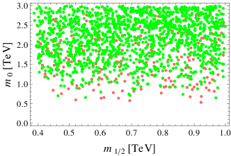
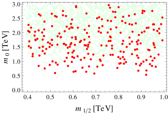
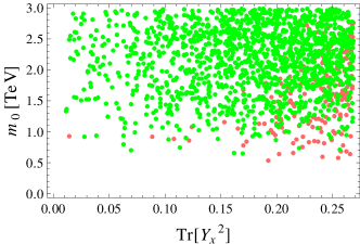
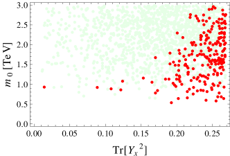
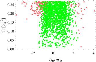
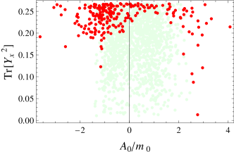
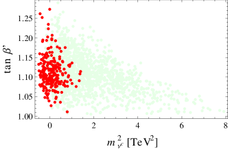
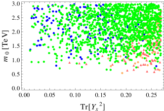
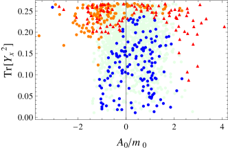
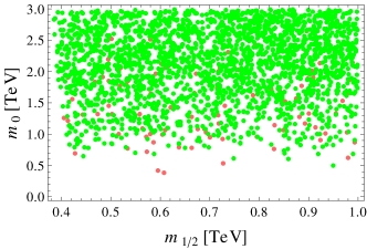
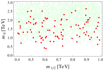
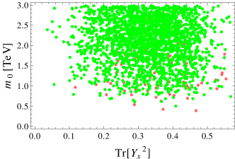
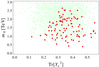
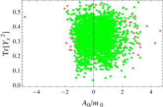
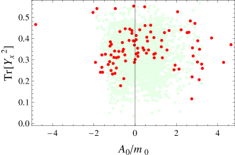
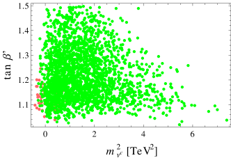
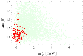
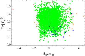
Figure 1: Projections into various parameter planes of the 1640 hierarchical scan parameter points, categorized by the nature of their global minima (see Tab. 3) at tree level. “RPC” points are plotted in green (light grey), and “RPV” points are plotted in red (medium grey). In the plots on the left, the “RPC” points are plotted on top of the “RPV” points, which are faded (very light grey), while in the plots on the right the “RPV” points are plotted on top of the “RPC” points, which are faded (very light grey). (mν~c2superscriptsubscript𝑚superscript~𝜈𝑐2{m_{{\tilde{\nu}}^{c}}^{2}} is the lowest or most negative of the three soft SUSY-breaking mass-squared parameters for the R-sneutrinos, evaluated at the SUSY scale.)
Refer to captionRefer to captionRefer to captionRefer to captionRefer to captionRefer to captionRefer to captionRefer to caption
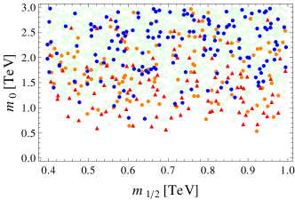
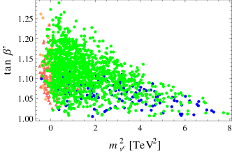
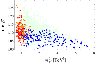
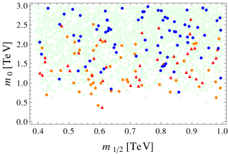
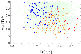
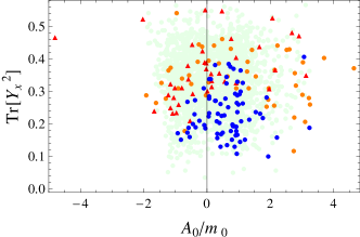
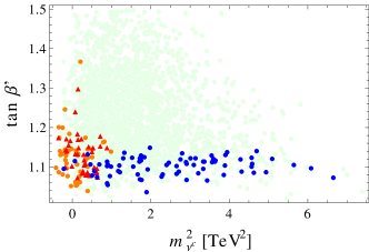
Figure 2: Projections into various parameter planes of the 1640 hierarchical scan parameter points, categorized by the nature of their global minima (see Tab. 3) at one-loop level. As in Fig. 1 “RPC” points are plotted in green (light grey), but now the “RPV” points are in two groups based on the tunneling time from the “RPC” input minimum to the deeper “RPV” minimum: lower than one tenth of the age of the Universe as orange (medium-light grey) circles, greater than a tenth of the age of the Universe as red (medium grey) triangles. “Gauge conserving” points are in blue (dark grey).
Refer to captionRefer to captionRefer to captionRefer to captionRefer to captionRefer to captionRefer to captionRefer to caption
Figure 3: Projections into various parameter planes of the 2330 democratic scan parameter points, categorized by the nature of their global minima (see Tab. 3) at tree level. The scheme is the same as in Fig. 1.
Refer to captionRefer to captionRefer to captionRefer to captionRefer to captionRefer to captionRefer to captionRefer to caption
Figure 4: Projections into various parameter planes of the 2330 democratic scan parameter points, categorized by the nature of their global minima (see Tab. 3) at one-loop level. The scheme is the same as in Fig. 2.

As can be seen in Figs. 1-4, there are R𝑅R-parity-conserving points all over the parameter space. Based purely on a tree-level analysis, one might conclude that there are clear regions where the BLSSM has a stable, R𝑅R-parity-conserving vacuum with the correct broken and unbroken gauge groups. These are, as one might expect, in regions where the R-sneutrino-bilepton Yukawa coupling Yxsubscript𝑌𝑥Y_{x} is not so large, and the trilinear soft SUSY-breaking parameter A0subscript𝐴0A_{0} is not large compared to the soft SUSY-breaking scalar mass parameter m0subscript𝑚0m_{0}, as, intuitively, large Yxsubscript𝑌𝑥Y_{x} and A0subscript𝐴0A_{0} can lead to large negative contributions to the potential energy for large values of vRsubscript𝑣𝑅v_{R} and vη/η¯subscript𝑣𝜂¯𝜂v_{\eta/\bar{\eta}}, as well as reducing the effective R-sneutrino mass term. Counter to this, a higher m0subscript𝑚0m_{0} leads to a higher mν2superscriptsubscript𝑚𝜈2m_{\nu}^{2} which, if positive, tends to penalize high vRsubscript𝑣𝑅v_{R} values. This pattern is seen in both the hierarchical and democratic sets. However, these conclusions run into trouble when loop corrections are taken into account: the regions where R𝑅R-parity appears to be safe at tree level apparently have very finely-tuned breaking of SU(2)L𝑆𝑈subscript2𝐿SU(2)_{L} and U(1)BL𝑈subscript1𝐵𝐿U(1)_{B-L} which often does not survive loop corrections. Hence, while parameter points often preserved R𝑅R-parity, there are points all over the region where the global vacuum is not the phenomenologically-acceptable vacuum given as input, and this other vacuum is not trivial to find. It turns out that besides the known large contributions of third generation sfermions and fermions, the additional new particles of the BL𝐵𝐿B-L sector also play an important role. The main reason for this is that the experimental bounds require mZsubscript𝑚superscript𝑍m_{Z^{\prime}} to be in the multi-TeV range, implying that vηsubscript𝑣𝜂v_{\eta} and vη¯subscript𝑣¯𝜂v_{\bar{\eta}} are also in this range. For tanβ1superscript𝛽1\tan\beta^{\prime}\neq 1 these VEVs give SUSY-breaking D-term contributions to the masses and, as they are much larger than the MSSM sector, this results in the observed importance of the corresponding loop contributions. These contributions are also responsible for the observed restoration of U(1)BL𝑈subscript1𝐵𝐿U(1)_{B-L} at the one-loop level. Moreover, as discussed in FileviezPerez:2010ek ; OLeary:2011yq at least one entry of Yxsubscript𝑌𝑥Y_{x} has to be large to achieve the breaking of U(1)BL𝑈subscript1𝐵𝐿U(1)_{B-L}. Here we have found that one-loop contributions due to the additional BL𝐵𝐿B-L sector are more important in the hierarchical case, driving a larger set of points from the global tree-level R𝑅R-parity-conserving minimum to the global R𝑅R-parity-violating minimum at one-loop level. The main reason for this is that now a single entry has to play the role of the trace and thus is correspondingly larger than the average of the democratic scan.

IV.1 Comparison with previous work

Previous studies on how much of the BLSSM parameter space conserves R𝑅R-parity FileviezPerez:2010ek considered the positivity of all the soft SUSY-breaking mass-squareds of the R-sneutrinos to be the necessary and sufficient condition. However, as can be seen in Figs. 2 and 4, this is neither necessary nor sufficient. There are, of course, obvious trends, and parameter points with very low or negative mν~c2superscriptsubscript𝑚superscript~𝜈𝑐2{m_{{\tilde{\nu}}^{c}}^{2}} are as likely to break R𝑅R-parity as conserve it, but there are clearly parameter points which conserve R𝑅R-parity despite having a negative mν~c2superscriptsubscript𝑚superscript~𝜈𝑐2{m_{{\tilde{\nu}}^{c}}^{2}}. This can be understood by the fact that one has to consider the eigenvalues of the mass matrix which can be all positive because of contributions of the F-terms, D-terms and other soft SUSY-breaking terms for non-zero bilepton VEVs despite negative mν~c2superscriptsubscript𝑚superscript~𝜈𝑐2{m_{{\tilde{\nu}}^{c}}^{2}} entries. For instance, the (ν~3c,ν~3c)subscriptsuperscript~𝜈𝑐3subscriptsuperscript~𝜈𝑐3({\tilde{\nu}}^{c}_{3},{\tilde{\nu}}^{c}_{3}) element of the tree-level scalar mass-squared matrix is given by

m(ν~3c,ν~3c)2subscriptsuperscript𝑚2subscriptsuperscript~𝜈𝑐3subscriptsuperscript~𝜈𝑐3\displaystyle m^{2}_{({\tilde{\nu}}^{c}_{3},{\tilde{\nu}}^{c}_{3})} =\displaystyle= mνc2+12(vL2+vu2)|Yν|22vη¯(Yxμ)+2vη(Tx)+(2vη2+3vR2)|Yx|2superscriptsubscript𝑚superscript𝜈𝑐212superscriptsubscript𝑣𝐿2superscriptsubscript𝑣𝑢2superscriptsubscript𝑌𝜈22subscript𝑣¯𝜂subscript𝑌𝑥superscript𝜇2subscript𝑣𝜂subscript𝑇𝑥2superscriptsubscript𝑣𝜂23superscriptsubscript𝑣𝑅2superscriptsubscript𝑌𝑥2\displaystyle m_{\nu^{c}}^{2}+\frac{1}{2}\left(v_{L}^{2}+v_{u}^{2}\right)|Y_{\nu}|^{2}-\sqrt{2}v_{\bar{\eta}}\Re\left(Y_{x}{\mu}^{\prime\ast}\right)+\sqrt{2}v_{\eta}\Re\left(T_{x}\right)+\left(2v_{\eta}^{2}+3v_{R}^{2}\right)|Y_{x}|^{2} (17)
+18(g¯gBL(vu2vd2vL2)+gBL2(2(vη¯2vη2)+3vR2vL2)).18¯𝑔subscript𝑔𝐵𝐿superscriptsubscript𝑣𝑢2superscriptsubscript𝑣𝑑2superscriptsubscript𝑣𝐿2superscriptsubscript𝑔𝐵𝐿22superscriptsubscript𝑣¯𝜂2superscriptsubscript𝑣𝜂23superscriptsubscript𝑣𝑅2superscriptsubscript𝑣𝐿2\displaystyle+\frac{1}{8}\Big{(}{\bar{g}}{g_{BL}}\left(v_{u}^{2}-v_{d}^{2}-v_{L}^{2}\right)+{g_{BL}^{2}}\left(2\left(v_{\bar{\eta}}^{2}-v_{\eta}^{2}\right)+3v_{R}^{2}-v_{L}^{2}\right)\Big{)}.

Parameter points that have all positive mν~c2superscriptsubscript𝑚superscript~𝜈𝑐2{m_{{\tilde{\nu}}^{c}}^{2}} yet still have R𝑅R-parity-violating global minima are less surprising, as the presence of trilinear terms obviously could dominate for reasonably large values of sneutrino and bilepton VEVs.

Furthermore, Ref. FileviezPerez:2010ek concluded that a hierarchical Yxsubscript𝑌𝑥Y_{x} would always break R𝑅R-parity, because of the way the couplings enter the RGEs and drive the soft SUSY-breaking sneutrino mass-squared parameters negative before the bilepton mass-squared parameters, unless all three generations contribute substantially. The large fraction of “RPC” points in our hierarchical scan refutes this claim. Such points are harder to find (as evidenced by the smaller size of the hierarchical scan to the democratic scan), and in some sense rather finely-tuned, as evidenced by the large fraction of “unbroken” points where loop corrections to the differences in potential are as large as the differences leading to the breaking of the symmetries at tree level. Still, almost half of the hierarchical points conserve R𝑅R-parity even at the one-loop level.

One should note, however, the different emphasis: we generated points that were naïvely R𝑅R-parity-conserving, and explored whether they had global minima elsewhere, which would break R𝑅R-parity or not break U(1)BL𝑈subscript1𝐵𝐿U(1)_{B-L} or SU(2)L𝑆𝑈subscript2𝐿SU(2)_{L}, scanning over both the soft SUSY-breaking parameters and the additional Yukawa couplings; Ref. FileviezPerez:2010ek explored various GUT-scale parameter configurations in the Yukawa sector for two points in the soft SUSY-breaking parameters to see whether RGE running would lead to a negative mν2superscriptsubscript𝑚𝜈2m_{\nu}^{2}. Since we started with a set of parameters engineered to have an R𝑅R-parity-conserving local minimum, perhaps it is not so surprising to find that we did not find as strong a tendency for R𝑅R-parity violation. However, we also feel that the criterion used in Ref. FileviezPerez:2010ek is not in perfect correspondance with whether or not the parameter point breaks or preserves R𝑅R-parity at its global minimum at the SUSY scale. Moreover, we have shown that loop effects do play an important role and should not be neglected.

Finally, we examined whether the “RPC” minima of the “RPV” points were long-lived with respect to the age of the Universe. Unfortunately there seem to be no clear correlations, as can be seen in Figs. 1 to 4; we note that the SUSY-scale sign of mν2superscriptsubscript𝑚𝜈2m_{\nu}^{2} appears to have little bearing even on the tunneling time from the “RPC” vacuum to the “RPV” vacuum.

V Conclusion

We have investigated the stability of R𝑅R-parity in a phenomenologically interesting region of the parameter space of the BLSSM by considering all the extrema of the tree-level potential and using the full one-loop evaluation of the potential at its extrema near those of the tree-level potential. We found that a significant fraction of points that were chosen to conserve R𝑅R-parity while having the correct mass for the weak vector bosons actually have global minima which violate R𝑅R-parity through non-zero sneutrino VEVs. However, we also found that more parameter points conserve R𝑅R-parity than violate it.

We also found that both the conservation and violation of R𝑅R-parity were possible all over the parameter space, in contradiction to previous studies, and while trends in the parameters leading either case are visible, it is difficult to identify in advance what values of which parameters will lead definitely to the conservation or violation of R𝑅R-parity.

Acknowledgments

This work has been supported by the DFG, project No. PO-1337/2-1, and partly by the Helmholtz alliance ‘Physics at the Terascale’. BO’L has been supported by DFG research training group GRK 1147.

Appendix A The one-loop effective potential

The effective potential at one-loop is calculated by using eq. (16) and reads in its full form:

16π216superscript𝜋2\displaystyle 16\pi^{2} (V1V0)=3(i=13(mdi44[ln(mdi2Q2)32])+i=13(mui44[ln(mui2Q2)32]))superscript𝑉1superscript𝑉03superscriptsubscript𝑖13subscriptsuperscript𝑚4subscript𝑑𝑖4delimited-[]𝑙𝑛subscriptsuperscript𝑚2subscript𝑑𝑖superscript𝑄232superscriptsubscript𝑖13subscriptsuperscript𝑚4subscript𝑢𝑖4delimited-[]𝑙𝑛subscriptsuperscript𝑚2subscript𝑢𝑖superscript𝑄232\displaystyle(V^{1}-V^{0})=-3\left(\sum_{i=1}^{3}\left(\frac{m^{4}_{d_{i}}}{4}\left[ln\left(\frac{m^{2}_{d_{i}}}{Q^{2}}\right)-\frac{3}{2}\right]\right)+\sum_{i=1}^{3}\left(\frac{m^{4}_{u_{i}}}{4}\left[ln\left(\frac{m^{2}_{u_{i}}}{Q^{2}}\right)-\frac{3}{2}\right]\right)\right)
+32(i=16(md~i44[ln(md~i2Q2)32])+i=16(mu~i44[ln(mu~i2Q2)32]))32superscriptsubscript𝑖16subscriptsuperscript𝑚4subscript~𝑑𝑖4delimited-[]𝑙𝑛subscriptsuperscript𝑚2subscript~𝑑𝑖superscript𝑄232superscriptsubscript𝑖16subscriptsuperscript𝑚4subscript~𝑢𝑖4delimited-[]𝑙𝑛subscriptsuperscript𝑚2subscript~𝑢𝑖superscript𝑄232\displaystyle+\frac{3}{2}\left(\sum_{i=1}^{6}\left(\frac{m^{4}_{\tilde{d}_{i}}}{4}\left[ln\left(\frac{m^{2}_{\tilde{d}_{i}}}{Q^{2}}\right)-\frac{3}{2}\right]\right)+\sum_{i=1}^{6}\left(\frac{m^{4}_{\tilde{u}_{i}}}{4}\left[ln\left(\frac{m^{2}_{\tilde{u}_{i}}}{Q^{2}}\right)-\frac{3}{2}\right]\right)\right)
+34(mW42[ln(mW2Q2)+32]+mZ44[ln(mZ2Q2)32]+mZ44[ln(mZ2Q2)32])34subscriptsuperscript𝑚4𝑊2delimited-[]𝑙𝑛subscriptsuperscript𝑚2𝑊superscript𝑄232subscriptsuperscript𝑚4𝑍4delimited-[]𝑙𝑛subscriptsuperscript𝑚2𝑍superscript𝑄232subscriptsuperscript𝑚4superscript𝑍4delimited-[]𝑙𝑛subscriptsuperscript𝑚2superscript𝑍superscript𝑄232\displaystyle+\frac{3}{4}\left(\frac{m^{4}_{W}}{2}\left[ln\left(\frac{m^{2}_{W}}{Q^{2}}\right)+\frac{3}{2}\right]+\frac{m^{4}_{Z}}{4}\left[ln\left(\frac{m^{2}_{Z}}{Q^{2}}\right)-\frac{3}{2}\right]+\frac{m^{4}_{Z^{\prime}}}{4}\left[ln\left(\frac{m^{2}_{Z^{\prime}}}{Q^{2}}\right)-\frac{3}{2}\right]\right)
i=15(mχ~i±44[ln(mχ~i±2Q2)32])12i=113(mχ~i044[ln(mχ~i02Q2)32])superscriptsubscript𝑖15subscriptsuperscript𝑚4subscriptsuperscript~𝜒plus-or-minus𝑖4delimited-[]𝑙𝑛subscriptsuperscript𝑚2subscriptsuperscript~𝜒plus-or-minus𝑖superscript𝑄23212superscriptsubscript𝑖113subscriptsuperscript𝑚4subscriptsuperscript~𝜒0𝑖4delimited-[]𝑙𝑛subscriptsuperscript𝑚2subscriptsuperscript~𝜒0𝑖superscript𝑄232\displaystyle-\sum_{i=1}^{5}\left(\frac{m^{4}_{\tilde{\chi}^{\pm}_{i}}}{4}\left[ln\left(\frac{m^{2}_{\tilde{\chi}^{\pm}_{i}}}{Q^{2}}\right)-\frac{3}{2}\right]\right)-\frac{1}{2}\sum_{i=1}^{13}\left(\frac{m^{4}_{\tilde{\chi}^{0}_{i}}}{4}\left[ln\left(\frac{m^{2}_{\tilde{\chi}^{0}_{i}}}{Q^{2}}\right)-\frac{3}{2}\right]\right)
+14(i=110(mhi44[ln(mhi2Q2)32])+i=110(mAi044[ln(mAi02Q2)32]))14superscriptsubscript𝑖110subscriptsuperscript𝑚4subscript𝑖4delimited-[]𝑙𝑛subscriptsuperscript𝑚2subscript𝑖superscript𝑄232superscriptsubscript𝑖110subscriptsuperscript𝑚4subscriptsuperscript𝐴0𝑖4delimited-[]𝑙𝑛subscriptsuperscript𝑚2subscriptsuperscript𝐴0𝑖superscript𝑄232\displaystyle+\frac{1}{4}\left(\sum_{i=1}^{10}\left(\frac{m^{4}_{h_{i}}}{4}\left[ln\left(\frac{m^{2}_{h_{i}}}{Q^{2}}\right)-\frac{3}{2}\right]\right)+\sum_{i=1}^{10}\left(\frac{m^{4}_{A^{0}_{i}}}{4}\left[ln\left(\frac{m^{2}_{A^{0}_{i}}}{Q^{2}}\right)-\frac{3}{2}\right]\right)\right)
+12i=18(me~i44[ln(me~i2Q2)32]).12superscriptsubscript𝑖18subscriptsuperscript𝑚4subscript~𝑒𝑖4delimited-[]𝑙𝑛subscriptsuperscript𝑚2subscript~𝑒𝑖superscript𝑄232\displaystyle+\frac{1}{2}\sum_{i=1}^{8}\left(\frac{m^{4}_{\tilde{e}_{i}}}{4}\left[ln\left(\frac{m^{2}_{\tilde{e}_{i}}}{Q^{2}}\right)-\frac{3}{2}\right]\right). (18)

The first two lines are the contributions from quarks and squarks which are the same as for the MSSM. In the third line the loops including the three gauge bosons in the given model are counted. The fourth line contains the contributions due to the charged lepton-chargino as well as neutrino-neutralino mixed states. The fifth and sixth lines show the contributions from charged slepton-charged Higgsino states as well as sneutrino-Higgs states. We have included formally in the sums the would-be Goldstone-bosons to account for the fact that potentially the gauge group is broken only partially. This does not result in a double-counting because, in the Landau gauge, would-be Goldstone-bosons are massless and thus give a zero contribution to the one-loop effective potential. The tree-level mass matrices where R𝑅R-parity violation induces a mixing between SM and SUSY particles are listed in appendix B. For completeness we note that in addition the sneutrino VEVs give contributions to the mass matrices of vector bosons and squarks.

Appendix B Mass matrices

Here we give the tree-level masses suppressing the generation indices of (s)neutrinos and (s)leptons.

  • Neutrino-Neutralino states
    The mass matrix mχ~02subscriptsuperscript𝑚2superscript~𝜒0m^{2}_{\tilde{\chi}^{0}} is given, in the basis

    (λB~,W~0,H~d0,H~u0,νL,νR,η~,η¯~,λB~),subscript𝜆~𝐵superscript~𝑊0superscriptsubscript~𝐻𝑑0superscriptsubscript~𝐻𝑢0subscript𝜈𝐿superscriptsubscript𝜈𝑅~𝜂~¯𝜂subscript𝜆~superscript𝐵\left(\lambda_{\tilde{B}},\tilde{W}^{0},\tilde{H}_{d}^{0},\tilde{H}_{u}^{0},\nu_{L},\nu_{R}^{*},\tilde{\eta},\tilde{\bar{\eta}},\lambda_{\tilde{B^{\prime}}}\right),

    by

    (M1012g1vd12g1vu12g1vL000MBB0M212g2vd12g2vu12g2vL000012g1vd12g2vd0μ000012g¯vd12g1vu12g2vuμ012vRYν12vLYν0012g¯vu12g1vL12g2vL012vRYν012vuYν0012(g¯+gB)vL00012vLYν12vuYν2vηYx2vRYx012gBvR000002vRYx0μgBvη000000μ0gBvη¯MBB012g¯vd12g¯vu12(g¯+gB)vL12gBvRgBvηgBvη¯MB).subscript𝑀1012subscript𝑔1subscript𝑣𝑑12subscript𝑔1subscript𝑣𝑢12subscript𝑔1subscript𝑣𝐿000subscript𝑀𝐵superscript𝐵0subscript𝑀212subscript𝑔2subscript𝑣𝑑12subscript𝑔2subscript𝑣𝑢12subscript𝑔2subscript𝑣𝐿000012subscript𝑔1subscript𝑣𝑑12subscript𝑔2subscript𝑣𝑑0𝜇000012¯𝑔subscript𝑣𝑑12subscript𝑔1subscript𝑣𝑢12subscript𝑔2subscript𝑣𝑢𝜇012subscript𝑣𝑅subscript𝑌𝜈12subscript𝑣𝐿subscript𝑌𝜈0012¯𝑔subscript𝑣𝑢12subscript𝑔1subscript𝑣𝐿12subscript𝑔2subscript𝑣𝐿012subscript𝑣𝑅subscript𝑌𝜈012subscript𝑣𝑢subscript𝑌𝜈0012¯𝑔subscript𝑔𝐵subscript𝑣𝐿00012subscript𝑣𝐿subscript𝑌𝜈12subscript𝑣𝑢subscript𝑌𝜈2subscript𝑣𝜂subscript𝑌𝑥2subscript𝑣𝑅subscript𝑌𝑥012subscript𝑔𝐵subscript𝑣𝑅000002subscript𝑣𝑅subscript𝑌𝑥0superscript𝜇subscript𝑔𝐵subscript𝑣𝜂000000superscript𝜇0subscript𝑔𝐵subscript𝑣¯𝜂subscript𝑀𝐵superscript𝐵012¯𝑔subscript𝑣𝑑12¯𝑔subscript𝑣𝑢12¯𝑔subscript𝑔𝐵subscript𝑣𝐿12subscript𝑔𝐵subscript𝑣𝑅subscript𝑔𝐵subscript𝑣𝜂subscript𝑔𝐵subscript𝑣¯𝜂subscript𝑀superscript𝐵\scriptscriptstyle{\left(\begin{array}[]{ccccccccc}M_{1}&0&-\frac{1}{2}g_{1}v_{d}&\frac{1}{2}g_{1}v_{u}&-\frac{1}{2}g_{1}v_{L}&0&0&0&{M}_{BB^{\prime}}\\ 0&M_{2}&\frac{1}{2}g_{2}v_{d}&-\frac{1}{2}g_{2}v_{u}&\frac{1}{2}g_{2}v_{L}&0&0&0&0\\ -\frac{1}{2}g_{1}v_{d}&\frac{1}{2}g_{2}v_{d}&0&-\mu&0&0&0&0&-\frac{1}{2}\bar{g}v_{d}\\ \frac{1}{2}g_{1}v_{u}&-\frac{1}{2}g_{2}v_{u}&-\mu&0&\frac{1}{\sqrt{2}}v_{R}Y_{\nu}&\frac{1}{\sqrt{2}}v_{L}Y_{\nu}&0&0&\frac{1}{2}\bar{g}v_{u}\\ -\frac{1}{2}g_{1}v_{L}&\frac{1}{2}g_{2}v_{L}&0&\frac{1}{\sqrt{2}}v_{R}Y_{\nu}&0&\frac{1}{\sqrt{2}}v_{u}Y_{\nu}&0&0&-\frac{1}{2}(\bar{g}+g_{B})v_{L}\\ 0&0&0&\frac{1}{\sqrt{2}}v_{L}Y_{\nu}&\frac{1}{\sqrt{2}}v_{u}Y_{\nu}&\sqrt{2}v_{\eta}Y_{x}&\sqrt{2}v_{R}Y_{x}&0&\frac{1}{2}g_{B}v_{R}\\ 0&0&0&0&0&\sqrt{2}v_{R}Y_{x}&0&-{\mu^{\prime}}&-g_{B}v_{\eta}\\ 0&0&0&0&0&0&-{\mu^{\prime}}&0&g_{B}v_{\bar{\eta}}\\ {M}_{BB^{\prime}}&0&-\frac{1}{2}\bar{g}v_{d}&\frac{1}{2}\bar{g}v_{u}&-\frac{1}{2}(\bar{g}+g_{B})v_{L}&\frac{1}{2}g_{B}v_{R}&-g_{B}v_{\eta}&g_{B}v_{\bar{\eta}}&{M}_{B^{\prime}}\end{array}\right)}. (19)
  • Charged lepton-Charginos
    The mass matrix is given, in the basis

    (eL,W~,H~d);(eR,W~+,H~u+),subscript𝑒𝐿superscript~𝑊superscriptsubscript~𝐻𝑑superscriptsubscript𝑒𝑅superscript~𝑊superscriptsubscript~𝐻𝑢\left(e_{L},\tilde{W}^{-},\tilde{H}_{d}^{-}\right);\left(e_{R}^{*},\tilde{W}^{+},\tilde{H}_{u}^{+}\right),

    by

    mχ~2=(12vdYe12g2vL12vRYν0M212g2vu12vLYe12g2vdμ).subscriptsuperscript𝑚2superscript~𝜒12subscript𝑣𝑑subscript𝑌𝑒12subscript𝑔2subscript𝑣𝐿12subscript𝑣𝑅subscript𝑌𝜈0subscript𝑀212subscript𝑔2subscript𝑣𝑢12subscript𝑣𝐿subscript𝑌𝑒12subscript𝑔2subscript𝑣𝑑𝜇m^{2}_{\tilde{\chi}^{-}}=\left(\begin{array}[]{ccc}\frac{1}{\sqrt{2}}v_{d}Y_{e}&\frac{1}{\sqrt{2}}g_{2}v_{L}&-\frac{1}{\sqrt{2}}v_{R}Y_{\nu}\\ 0&M_{2}&\frac{1}{\sqrt{2}}g_{2}v_{u}\\ -\frac{1}{\sqrt{2}}v_{L}Y_{e}&\frac{1}{\sqrt{2}}g_{2}v_{d}&\mu\end{array}\right). (20)
  • CP even sneutrino-Higgs
    In the basis

    (σd,σu,σL,σR,ση,ση¯),subscript𝜎𝑑subscript𝜎𝑢subscript𝜎𝐿subscript𝜎𝑅subscript𝜎𝜂subscript𝜎¯𝜂\left(\sigma_{d},\sigma_{u},\sigma_{L},\sigma_{R},\sigma_{\eta},\sigma_{\bar{\eta}}\right),

    the entries of the mass matrix read:

    mσdσdsubscript𝑚subscript𝜎𝑑subscript𝜎𝑑\displaystyle m_{\sigma_{d}\sigma_{d}} =18(g¯gBL(2vη22vη¯2vR2+vL2)+(g12+g¯2+g22)(3vd2vu2+vL2))+mHd2+μ2absent18¯𝑔subscript𝑔𝐵𝐿2superscriptsubscript𝑣𝜂22superscriptsubscript𝑣¯𝜂2superscriptsubscript𝑣𝑅2superscriptsubscript𝑣𝐿2superscriptsubscript𝑔12superscript¯𝑔2superscriptsubscript𝑔223superscriptsubscript𝑣𝑑2superscriptsubscript𝑣𝑢2superscriptsubscript𝑣𝐿2superscriptsubscript𝑚subscript𝐻𝑑2superscript𝜇2\displaystyle=\frac{1}{8}\Big{(}\bar{g}g_{BL}\Big{(}2v_{\eta}^{2}-2v_{\bar{\eta}}^{2}-v_{R}^{2}+v_{L}^{2}\Big{)}+\Big{(}g_{1}^{2}+\bar{g}^{2}+g_{2}^{2}\Big{)}\Big{(}3v_{d}^{2}-v_{u}^{2}+v_{L}^{2}\Big{)}\Big{)}+m_{H_{d}}^{2}+\mu^{2} (21)
    mσdσusubscript𝑚subscript𝜎𝑑subscript𝜎𝑢\displaystyle m_{\sigma_{d}\sigma_{u}} =Bμ14(g12+g¯2+g22)vdvuabsentsubscript𝐵𝜇14superscriptsubscript𝑔12superscript¯𝑔2superscriptsubscript𝑔22subscript𝑣𝑑subscript𝑣𝑢\displaystyle=-B_{\mu}-\frac{1}{4}\Big{(}g_{1}^{2}+\bar{g}^{2}+g_{2}^{2}\Big{)}v_{d}v_{u} (22)
    mσuσusubscript𝑚subscript𝜎𝑢subscript𝜎𝑢\displaystyle m_{\sigma_{u}\sigma_{u}} =mHu2+18((g¯2g12g22)(vd23vu2+vL2)+g¯gBL(2vη¯22vη2vL2+vR2))absentsuperscriptsubscript𝑚subscript𝐻𝑢218superscript¯𝑔2superscriptsubscript𝑔12superscriptsubscript𝑔22superscriptsubscript𝑣𝑑23superscriptsubscript𝑣𝑢2superscriptsubscript𝑣𝐿2¯𝑔subscript𝑔𝐵𝐿2superscriptsubscript𝑣¯𝜂22superscriptsubscript𝑣𝜂2superscriptsubscript𝑣𝐿2superscriptsubscript𝑣𝑅2\displaystyle=m_{H_{u}}^{2}+\frac{1}{8}\Big{(}\Big{(}-\bar{g}^{2}-g_{1}^{2}-g_{2}^{2}\Big{)}\Big{(}v_{d}^{2}-3v_{u}^{2}+v_{L}^{2}\Big{)}+\bar{g}g_{BL}\Big{(}2v_{\bar{\eta}}^{2}-2v_{\eta}^{2}-v_{L}^{2}+v_{R}^{2}\Big{)}\Big{)}
    +12(vL2+vR2)Yν2+μ212superscriptsubscript𝑣𝐿2superscriptsubscript𝑣𝑅2superscriptsubscript𝑌𝜈2superscript𝜇2\displaystyle+\frac{1}{2}\Big{(}v_{L}^{2}+v_{R}^{2}\Big{)}Y_{\nu}^{2}+\mu^{2} (23)
    mσdσLsubscript𝑚subscript𝜎𝑑subscript𝜎𝐿\displaystyle m_{\sigma_{d}\sigma_{L}} =14(g¯(g¯+gBL)+g12+g22)vdvL12vRYνμabsent14¯𝑔¯𝑔subscript𝑔𝐵𝐿superscriptsubscript𝑔12superscriptsubscript𝑔22subscript𝑣𝑑subscript𝑣𝐿12subscript𝑣𝑅subscript𝑌𝜈𝜇\displaystyle=\frac{1}{4}\Big{(}\bar{g}\Big{(}\bar{g}+g_{BL}\Big{)}+g_{1}^{2}+g_{2}^{2}\Big{)}v_{d}v_{L}-\frac{1}{\sqrt{2}}v_{R}Y_{\nu}\mu (24)
    mσuσLsubscript𝑚subscript𝜎𝑢subscript𝜎𝐿\displaystyle m_{\sigma_{u}\sigma_{L}} =14(g¯(g¯+gBL)+g12+g22)vLvu+12vRTν+Yν(vLvuYν+vRvηYx)absent14¯𝑔¯𝑔subscript𝑔𝐵𝐿superscriptsubscript𝑔12superscriptsubscript𝑔22subscript𝑣𝐿subscript𝑣𝑢12subscript𝑣𝑅subscript𝑇𝜈subscript𝑌𝜈subscript𝑣𝐿subscript𝑣𝑢subscript𝑌𝜈subscript𝑣𝑅subscript𝑣𝜂subscript𝑌𝑥\displaystyle=-\frac{1}{4}\Big{(}\bar{g}\Big{(}\bar{g}+g_{BL}\Big{)}+g_{1}^{2}+g_{2}^{2}\Big{)}v_{L}v_{u}+\frac{1}{\sqrt{2}}v_{R}T_{\nu}+Y_{\nu}\Big{(}v_{L}v_{u}Y_{\nu}+v_{R}v_{\eta}Y_{x}\Big{)} (25)
    mσLσLsubscript𝑚subscript𝜎𝐿subscript𝜎𝐿\displaystyle m_{\sigma_{L}\sigma_{L}} =mL2+18((g12+g¯2+g22)(3vL2vu2+vd2)+gBL2(2vη¯2+2vη2+3vL2vR2)\displaystyle=m_{L}^{2}+\frac{1}{8}\Big{(}\Big{(}g_{1}^{2}+\bar{g}^{2}+g_{2}^{2}\Big{)}\Big{(}3v_{L}^{2}-v_{u}^{2}+v_{d}^{2}\Big{)}+g_{BL}^{2}\Big{(}-2v_{\bar{\eta}}^{2}+2v_{\eta}^{2}+3v_{L}^{2}-v_{R}^{2}\Big{)}
    +g¯gBL(2vη¯2+2vη2+6vL2vR2vu2+vd2))+12(vR2+vu2)Yν2\displaystyle+\bar{g}g_{BL}\Big{(}-2v_{\bar{\eta}}^{2}+2v_{\eta}^{2}+6v_{L}^{2}-v_{R}^{2}-v_{u}^{2}+v_{d}^{2}\Big{)}\Big{)}+\frac{1}{2}\Big{(}v_{R}^{2}+v_{u}^{2}\Big{)}Y_{\nu}^{2} (26)
    mσdσRsubscript𝑚subscript𝜎𝑑subscript𝜎𝑅\displaystyle m_{\sigma_{d}\sigma_{R}} =14g¯gBLvdvR12vLYνμabsent14¯𝑔subscript𝑔𝐵𝐿subscript𝑣𝑑subscript𝑣𝑅12subscript𝑣𝐿subscript𝑌𝜈𝜇\displaystyle=-\frac{1}{4}\bar{g}g_{BL}v_{d}v_{R}-\frac{1}{\sqrt{2}}v_{L}Y_{\nu}\mu (27)
    mσuσRsubscript𝑚subscript𝜎𝑢subscript𝜎𝑅\displaystyle m_{\sigma_{u}\sigma_{R}} =14g¯gBLvRvu+12vLTν+Yν(vLvηYx+vRvuYν)absent14¯𝑔subscript𝑔𝐵𝐿subscript𝑣𝑅subscript𝑣𝑢12subscript𝑣𝐿subscript𝑇𝜈subscript𝑌𝜈subscript𝑣𝐿subscript𝑣𝜂subscript𝑌𝑥subscript𝑣𝑅subscript𝑣𝑢subscript𝑌𝜈\displaystyle=\frac{1}{4}\bar{g}g_{BL}v_{R}v_{u}+\frac{1}{\sqrt{2}}v_{L}T_{\nu}+Y_{\nu}\Big{(}v_{L}v_{\eta}Y_{x}+v_{R}v_{u}Y_{\nu}\Big{)} (28)
    mσLσRsubscript𝑚subscript𝜎𝐿subscript𝜎𝑅\displaystyle m_{\sigma_{L}\sigma_{R}} =14gBL(g¯+gBL)vLvR+12vuTν+vLvRYν2+Yν(12vdμ+vuvηYx)absent14subscript𝑔𝐵𝐿¯𝑔subscript𝑔𝐵𝐿subscript𝑣𝐿subscript𝑣𝑅12subscript𝑣𝑢subscript𝑇𝜈subscript𝑣𝐿subscript𝑣𝑅superscriptsubscript𝑌𝜈2subscript𝑌𝜈12subscript𝑣𝑑𝜇subscript𝑣𝑢subscript𝑣𝜂subscript𝑌𝑥\displaystyle=-\frac{1}{4}g_{BL}\Big{(}\bar{g}+g_{BL}\Big{)}v_{L}v_{R}+\frac{1}{\sqrt{2}}v_{u}T_{\nu}+v_{L}v_{R}Y_{\nu}^{2}+Y_{\nu}\Big{(}-\frac{1}{\sqrt{2}}v_{d}\mu+v_{u}v_{\eta}Y_{x}\Big{)} (29)
    mσRσRsubscript𝑚subscript𝜎𝑅subscript𝜎𝑅\displaystyle m_{\sigma_{R}\sigma_{R}} =mνc218gBL(g¯(vu2+vd2+vL2)+gBL(2vη¯2+2vη23vR2+vL2))absentsuperscriptsubscript𝑚superscript𝜈𝑐218subscript𝑔𝐵𝐿¯𝑔superscriptsubscript𝑣𝑢2superscriptsubscript𝑣𝑑2superscriptsubscript𝑣𝐿2subscript𝑔𝐵𝐿2superscriptsubscript𝑣¯𝜂22superscriptsubscript𝑣𝜂23superscriptsubscript𝑣𝑅2superscriptsubscript𝑣𝐿2\displaystyle={m_{\nu^{c}}^{2}}-\frac{1}{8}g_{BL}\Big{(}\bar{g}\Big{(}-v_{u}^{2}+v_{d}^{2}+v_{L}^{2}\Big{)}+g_{BL}\Big{(}-2v_{\bar{\eta}}^{2}+2v_{\eta}^{2}-3v_{R}^{2}+v_{L}^{2}\Big{)}\Big{)}
    +12(2(2vηTx+Yx((2vη2+3vR2)Yx2μvη¯))+(vL2+vu2)Yν2)1222subscript𝑣𝜂subscript𝑇𝑥subscript𝑌𝑥2superscriptsubscript𝑣𝜂23superscriptsubscript𝑣𝑅2subscript𝑌𝑥2superscript𝜇subscript𝑣¯𝜂superscriptsubscript𝑣𝐿2superscriptsubscript𝑣𝑢2superscriptsubscript𝑌𝜈2\displaystyle+\frac{1}{2}\Big{(}2\Big{(}\sqrt{2}v_{\eta}T_{x}+Y_{x}\Big{(}\Big{(}2v_{\eta}^{2}+3v_{R}^{2}\Big{)}Y_{x}-\sqrt{2}{\mu^{\prime}}v_{\bar{\eta}}\Big{)}\Big{)}+\Big{(}v_{L}^{2}+v_{u}^{2}\Big{)}Y_{\nu}^{2}\Big{)} (30)
    mσdσηsubscript𝑚subscript𝜎𝑑subscript𝜎𝜂\displaystyle m_{\sigma_{d}\sigma_{\eta}} =12g¯gBLvdvηabsent12¯𝑔subscript𝑔𝐵𝐿subscript𝑣𝑑subscript𝑣𝜂\displaystyle=\frac{1}{2}\bar{g}g_{BL}v_{d}v_{\eta} (31)
    mσuσηsubscript𝑚subscript𝜎𝑢subscript𝜎𝜂\displaystyle m_{\sigma_{u}\sigma_{\eta}} =12g¯gBLvuvη+vLvRYxYνabsent12¯𝑔subscript𝑔𝐵𝐿subscript𝑣𝑢subscript𝑣𝜂subscript𝑣𝐿subscript𝑣𝑅subscript𝑌𝑥subscript𝑌𝜈\displaystyle=-\frac{1}{2}\bar{g}g_{BL}v_{u}v_{\eta}+v_{L}v_{R}Y_{x}Y_{\nu} (32)
    mσLσηsubscript𝑚subscript𝜎𝐿subscript𝜎𝜂\displaystyle m_{\sigma_{L}\sigma_{\eta}} =12gBL(g¯+gBL)vLvη+vRvuYxYνabsent12subscript𝑔𝐵𝐿¯𝑔subscript𝑔𝐵𝐿subscript𝑣𝐿subscript𝑣𝜂subscript𝑣𝑅subscript𝑣𝑢subscript𝑌𝑥subscript𝑌𝜈\displaystyle=\frac{1}{2}g_{BL}\Big{(}\bar{g}+g_{BL}\Big{)}v_{L}v_{\eta}+v_{R}v_{u}Y_{x}Y_{\nu} (33)
    mσRσηsubscript𝑚subscript𝜎𝑅subscript𝜎𝜂\displaystyle m_{\sigma_{R}\sigma_{\eta}} =12gBL2vRvη+2vRTx+Yx(4vRvηYx+vLvuYν)absent12superscriptsubscript𝑔𝐵𝐿2subscript𝑣𝑅subscript𝑣𝜂2subscript𝑣𝑅subscript𝑇𝑥subscript𝑌𝑥4subscript𝑣𝑅subscript𝑣𝜂subscript𝑌𝑥subscript𝑣𝐿subscript𝑣𝑢subscript𝑌𝜈\displaystyle=-\frac{1}{2}g_{BL}^{2}v_{R}v_{\eta}+\sqrt{2}v_{R}T_{x}+Y_{x}\Big{(}4v_{R}v_{\eta}Y_{x}+v_{L}v_{u}Y_{\nu}\Big{)} (34)
    mσησηsubscript𝑚subscript𝜎𝜂subscript𝜎𝜂\displaystyle m_{\sigma_{\eta}\sigma_{\eta}} =2vR2Yx2+14gBL(g¯(vd2vu2+vL2)+gBL(6vη22vη¯2vR2+vL2))+mη2+μ2absent2superscriptsubscript𝑣𝑅2superscriptsubscript𝑌𝑥214subscript𝑔𝐵𝐿¯𝑔superscriptsubscript𝑣𝑑2superscriptsubscript𝑣𝑢2superscriptsubscript𝑣𝐿2subscript𝑔𝐵𝐿6superscriptsubscript𝑣𝜂22superscriptsubscript𝑣¯𝜂2superscriptsubscript𝑣𝑅2superscriptsubscript𝑣𝐿2superscriptsubscript𝑚𝜂2superscriptsuperscript𝜇2\displaystyle=2v_{R}^{2}Y_{x}^{2}+\frac{1}{4}g_{BL}\Big{(}\bar{g}\Big{(}v_{d}^{2}-v_{u}^{2}+v_{L}^{2}\Big{)}+g_{BL}\Big{(}6v_{\eta}^{2}-2v_{\bar{\eta}}^{2}-v_{R}^{2}+v_{L}^{2}\Big{)}\Big{)}+m_{\eta}^{2}+{\mu^{\prime}}^{2} (35)
    mσdση¯subscript𝑚subscript𝜎𝑑subscript𝜎¯𝜂\displaystyle m_{\sigma_{d}\sigma_{\bar{\eta}}} =12g¯gBLvdvη¯absent12¯𝑔subscript𝑔𝐵𝐿subscript𝑣𝑑subscript𝑣¯𝜂\displaystyle=-\frac{1}{2}\bar{g}g_{BL}v_{d}v_{\bar{\eta}} (36)
    mσuση¯subscript𝑚subscript𝜎𝑢subscript𝜎¯𝜂\displaystyle m_{\sigma_{u}\sigma_{\bar{\eta}}} =12g¯gBLvuvη¯absent12¯𝑔subscript𝑔𝐵𝐿subscript𝑣𝑢subscript𝑣¯𝜂\displaystyle=\frac{1}{2}\bar{g}g_{BL}v_{u}v_{\bar{\eta}} (37)
    mσLση¯subscript𝑚subscript𝜎𝐿subscript𝜎¯𝜂\displaystyle m_{\sigma_{L}\sigma_{\bar{\eta}}} =12gBL(g¯+gBL)vLvη¯absent12subscript𝑔𝐵𝐿¯𝑔subscript𝑔𝐵𝐿subscript𝑣𝐿subscript𝑣¯𝜂\displaystyle=-\frac{1}{2}g_{BL}\Big{(}\bar{g}+g_{BL}\Big{)}v_{L}v_{\bar{\eta}} (38)
    mσRση¯subscript𝑚subscript𝜎𝑅subscript𝜎¯𝜂\displaystyle m_{\sigma_{R}\sigma_{\bar{\eta}}} =12gBL2vRvη¯2μvRYxabsent12superscriptsubscript𝑔𝐵𝐿2subscript𝑣𝑅subscript𝑣¯𝜂2superscript𝜇subscript𝑣𝑅subscript𝑌𝑥\displaystyle=\frac{1}{2}g_{BL}^{2}v_{R}v_{\bar{\eta}}-\sqrt{2}{\mu^{\prime}}v_{R}Y_{x} (39)
    mσηση¯subscript𝑚subscript𝜎𝜂subscript𝜎¯𝜂\displaystyle m_{\sigma_{\eta}\sigma_{\bar{\eta}}} =BμgBL2vηvη¯absentsubscript𝐵superscript𝜇superscriptsubscript𝑔𝐵𝐿2subscript𝑣𝜂subscript𝑣¯𝜂\displaystyle=-{B_{\mu^{\prime}}}-g_{BL}^{2}v_{\eta}v_{\bar{\eta}} (40)
    mση¯ση¯subscript𝑚subscript𝜎¯𝜂subscript𝜎¯𝜂\displaystyle m_{\sigma_{\bar{\eta}}\sigma_{\bar{\eta}}} =14gBL(g¯(vu2+vd2+vL2)+gBL(2vη26vη¯2vR2+vL2))+mη¯2+μ2absent14subscript𝑔𝐵𝐿¯𝑔superscriptsubscript𝑣𝑢2superscriptsubscript𝑣𝑑2superscriptsubscript𝑣𝐿2subscript𝑔𝐵𝐿2superscriptsubscript𝑣𝜂26superscriptsubscript𝑣¯𝜂2superscriptsubscript𝑣𝑅2superscriptsubscript𝑣𝐿2superscriptsubscript𝑚¯𝜂2superscriptsuperscript𝜇2\displaystyle=-\frac{1}{4}g_{BL}\Big{(}\bar{g}\Big{(}-v_{u}^{2}+v_{d}^{2}+v_{L}^{2}\Big{)}+g_{BL}\Big{(}2v_{\eta}^{2}-6v_{\bar{\eta}}^{2}-v_{R}^{2}+v_{L}^{2}\Big{)}\Big{)}+m_{\bar{\eta}}^{2}+{\mu^{\prime}}^{2} (41)
  • CP odd sneutrino-Higgs
    In the basis (ϕd,ϕu,ϕL,ϕR,ϕη,ϕη¯)subscriptitalic-ϕ𝑑subscriptitalic-ϕ𝑢subscriptitalic-ϕ𝐿subscriptitalic-ϕ𝑅subscriptitalic-ϕ𝜂subscriptitalic-ϕ¯𝜂\left(\phi_{d},\phi_{u},\phi_{L},\phi_{R},\phi_{\eta},\phi_{\bar{\eta}}\right) and using Landau gauge, the nonzero entries of the mass matrix read:

    mϕdϕdsubscript𝑚subscriptitalic-ϕ𝑑subscriptitalic-ϕ𝑑\displaystyle m_{\phi_{d}\phi_{d}} =18(g¯gBL(2(vη2vη¯2)vR2+vL2)+(g12+g¯2+g22)(vd2vu2+vL2))+mHd2+μ2absent18¯𝑔subscript𝑔𝐵𝐿2superscriptsubscript𝑣𝜂2superscriptsubscript𝑣¯𝜂2superscriptsubscript𝑣𝑅2superscriptsubscript𝑣𝐿2superscriptsubscript𝑔12superscript¯𝑔2superscriptsubscript𝑔22superscriptsubscript𝑣𝑑2superscriptsubscript𝑣𝑢2superscriptsubscript𝑣𝐿2superscriptsubscript𝑚subscript𝐻𝑑2superscript𝜇2\displaystyle=\frac{1}{8}\Big{(}\bar{g}g_{BL}\Big{(}2\Big{(}v_{\eta}^{2}-v_{\bar{\eta}}^{2}\Big{)}-v_{R}^{2}+v_{L}^{2}\Big{)}+\Big{(}g_{1}^{2}+\bar{g}^{2}+g_{2}^{2}\Big{)}\Big{(}v_{d}^{2}-v_{u}^{2}+v_{L}^{2}\Big{)}\Big{)}+m_{H_{d}}^{2}+\mu^{2} (42)
    mϕdϕusubscript𝑚subscriptitalic-ϕ𝑑subscriptitalic-ϕ𝑢\displaystyle m_{\phi_{d}\phi_{u}} =Bμabsentsubscript𝐵𝜇\displaystyle=B_{\mu} (43)
    mϕuϕusubscript𝑚subscriptitalic-ϕ𝑢subscriptitalic-ϕ𝑢\displaystyle m_{\phi_{u}\phi_{u}} =mHu2+18((g¯2g12g22)(vu2+vd2+vL2)+g¯gBL(2vη¯22vη2vL2+vR2))absentsuperscriptsubscript𝑚subscript𝐻𝑢218superscript¯𝑔2superscriptsubscript𝑔12superscriptsubscript𝑔22superscriptsubscript𝑣𝑢2superscriptsubscript𝑣𝑑2superscriptsubscript𝑣𝐿2¯𝑔subscript𝑔𝐵𝐿2superscriptsubscript𝑣¯𝜂22superscriptsubscript𝑣𝜂2superscriptsubscript𝑣𝐿2superscriptsubscript𝑣𝑅2\displaystyle=m_{H_{u}}^{2}+\frac{1}{8}\Big{(}\Big{(}-\bar{g}^{2}-g_{1}^{2}-g_{2}^{2}\Big{)}\Big{(}-v_{u}^{2}+v_{d}^{2}+v_{L}^{2}\Big{)}+\bar{g}g_{BL}\Big{(}2v_{\bar{\eta}}^{2}-2v_{\eta}^{2}-v_{L}^{2}+v_{R}^{2}\Big{)}\Big{)}
    +12(vL2+vR2)Yν2+μ212superscriptsubscript𝑣𝐿2superscriptsubscript𝑣𝑅2superscriptsubscript𝑌𝜈2superscript𝜇2\displaystyle+\frac{1}{2}\Big{(}v_{L}^{2}+v_{R}^{2}\Big{)}Y_{\nu}^{2}+\mu^{2} (44)
    mϕdϕLsubscript𝑚subscriptitalic-ϕ𝑑subscriptitalic-ϕ𝐿\displaystyle m_{\phi_{d}\phi_{L}} =12vRYνμabsent12subscript𝑣𝑅subscript𝑌𝜈𝜇\displaystyle=-\frac{1}{\sqrt{2}}v_{R}Y_{\nu}\mu (45)
    mϕuϕLsubscript𝑚subscriptitalic-ϕ𝑢subscriptitalic-ϕ𝐿\displaystyle m_{\phi_{u}\phi_{L}} =12vR(2vηYxYν+2Tν)absent12subscript𝑣𝑅2subscript𝑣𝜂subscript𝑌𝑥subscript𝑌𝜈2subscript𝑇𝜈\displaystyle=-\frac{1}{2}v_{R}\Big{(}2v_{\eta}Y_{x}Y_{\nu}+\sqrt{2}T_{\nu}\Big{)} (46)
    mϕLϕLsubscript𝑚subscriptitalic-ϕ𝐿subscriptitalic-ϕ𝐿\displaystyle m_{\phi_{L}\phi_{L}} =mL2+18((g12+g¯2+g22)(vd2vu2+vL2)+g¯gBL(2(vL2+vη2vη¯2)vR2vu2+vd2)\displaystyle=m_{L}^{2}+\frac{1}{8}\Big{(}\Big{(}g_{1}^{2}+\bar{g}^{2}+g_{2}^{2}\Big{)}\Big{(}v_{d}^{2}-v_{u}^{2}+v_{L}^{2}\Big{)}+\bar{g}g_{BL}\Big{(}2\Big{(}v_{L}^{2}+v_{\eta}^{2}-v_{\bar{\eta}}^{2}\Big{)}-v_{R}^{2}-v_{u}^{2}+v_{d}^{2}\Big{)}
    +gBL2(2(vη¯2+vη2)vR2+vL2))+12(vR2+vu2)Yν2\displaystyle+g_{BL}^{2}\Big{(}2\Big{(}-v_{\bar{\eta}}^{2}+v_{\eta}^{2}\Big{)}-v_{R}^{2}+v_{L}^{2}\Big{)}\Big{)}+\frac{1}{2}\Big{(}v_{R}^{2}+v_{u}^{2}\Big{)}Y_{\nu}^{2} (47)
    mϕdϕRsubscript𝑚subscriptitalic-ϕ𝑑subscriptitalic-ϕ𝑅\displaystyle m_{\phi_{d}\phi_{R}} =12vLYνμabsent12subscript𝑣𝐿subscript𝑌𝜈𝜇\displaystyle=-\frac{1}{\sqrt{2}}v_{L}Y_{\nu}\mu (48)
    mϕuϕRsubscript𝑚subscriptitalic-ϕ𝑢subscriptitalic-ϕ𝑅\displaystyle m_{\phi_{u}\phi_{R}} =vL(12TνvηYxYν)absentsubscript𝑣𝐿12subscript𝑇𝜈subscript𝑣𝜂subscript𝑌𝑥subscript𝑌𝜈\displaystyle=v_{L}\Big{(}\frac{1}{\sqrt{2}}T_{\nu}-v_{\eta}Y_{x}Y_{\nu}\Big{)} (49)
    mϕLϕRsubscript𝑚subscriptitalic-ϕ𝐿subscriptitalic-ϕ𝑅\displaystyle m_{\phi_{L}\phi_{R}} =12vuTν+Yν(12vdμvuvηYx)absent12subscript𝑣𝑢subscript𝑇𝜈subscript𝑌𝜈12subscript𝑣𝑑𝜇subscript𝑣𝑢subscript𝑣𝜂subscript𝑌𝑥\displaystyle=\frac{1}{\sqrt{2}}v_{u}T_{\nu}+Y_{\nu}\Big{(}-\frac{1}{\sqrt{2}}v_{d}\mu-v_{u}v_{\eta}Y_{x}\Big{)} (50)
    mϕRϕRsubscript𝑚subscriptitalic-ϕ𝑅subscriptitalic-ϕ𝑅\displaystyle m_{\phi_{R}\phi_{R}} =mνc2+18gBL(g¯(vu2+vd2+vL2)+gBL(2vη¯22vη2vL2+vR2))absentsuperscriptsubscript𝑚superscript𝜈𝑐218subscript𝑔𝐵𝐿¯𝑔superscriptsubscript𝑣𝑢2superscriptsubscript𝑣𝑑2superscriptsubscript𝑣𝐿2subscript𝑔𝐵𝐿2superscriptsubscript𝑣¯𝜂22superscriptsubscript𝑣𝜂2superscriptsubscript𝑣𝐿2superscriptsubscript𝑣𝑅2\displaystyle={m_{\nu^{c}}^{2}}+\frac{1}{8}g_{BL}\Big{(}-\bar{g}\Big{(}-v_{u}^{2}+v_{d}^{2}+v_{L}^{2}\Big{)}+g_{BL}\Big{(}2v_{\bar{\eta}}^{2}-2v_{\eta}^{2}-v_{L}^{2}+v_{R}^{2}\Big{)}\Big{)}
    +12(22vηTx+2Yx((2vη2+vR2)Yx+2μvη¯)+(vL2+vu2)Yν2)1222subscript𝑣𝜂subscript𝑇𝑥2subscript𝑌𝑥2superscriptsubscript𝑣𝜂2superscriptsubscript𝑣𝑅2subscript𝑌𝑥2superscript𝜇subscript𝑣¯𝜂superscriptsubscript𝑣𝐿2superscriptsubscript𝑣𝑢2superscriptsubscript𝑌𝜈2\displaystyle+\frac{1}{2}\Big{(}-2\sqrt{2}v_{\eta}T_{x}+2Y_{x}\Big{(}\Big{(}2v_{\eta}^{2}+v_{R}^{2}\Big{)}Y_{x}+\sqrt{2}{\mu^{\prime}}v_{\bar{\eta}}\Big{)}+\Big{(}v_{L}^{2}+v_{u}^{2}\Big{)}Y_{\nu}^{2}\Big{)} (51)
    mϕuϕηsubscript𝑚subscriptitalic-ϕ𝑢subscriptitalic-ϕ𝜂\displaystyle m_{\phi_{u}\phi_{\eta}} =vLvRYxYνabsentsubscript𝑣𝐿subscript𝑣𝑅subscript𝑌𝑥subscript𝑌𝜈\displaystyle=v_{L}v_{R}Y_{x}Y_{\nu} (52)
    mϕLϕηsubscript𝑚subscriptitalic-ϕ𝐿subscriptitalic-ϕ𝜂\displaystyle m_{\phi_{L}\phi_{\eta}} =vRvuYxYνabsentsubscript𝑣𝑅subscript𝑣𝑢subscript𝑌𝑥subscript𝑌𝜈\displaystyle=v_{R}v_{u}Y_{x}Y_{\nu} (53)
    mϕRϕηsubscript𝑚subscriptitalic-ϕ𝑅subscriptitalic-ϕ𝜂\displaystyle m_{\phi_{R}\phi_{\eta}} =2vRTx+vLvuYxYνabsent2subscript𝑣𝑅subscript𝑇𝑥subscript𝑣𝐿subscript𝑣𝑢subscript𝑌𝑥subscript𝑌𝜈\displaystyle=\sqrt{2}v_{R}T_{x}+v_{L}v_{u}Y_{x}Y_{\nu} (54)
    mϕRϕη¯subscript𝑚subscriptitalic-ϕ𝑅subscriptitalic-ϕ¯𝜂\displaystyle m_{\phi_{R}\phi_{\bar{\eta}}} =2μvRYxabsent2superscript𝜇subscript𝑣𝑅subscript𝑌𝑥\displaystyle=\sqrt{2}{\mu^{\prime}}v_{R}Y_{x} (55)
    mϕηϕηsubscript𝑚subscriptitalic-ϕ𝜂subscriptitalic-ϕ𝜂\displaystyle m_{\phi_{\eta}\phi_{\eta}} =2vR2Yx2+14gBL(g¯(vd2vu2+vL2)+gBL(2(vη2vη¯2)vR2+vL2))+mη2+μ2absent2superscriptsubscript𝑣𝑅2superscriptsubscript𝑌𝑥214subscript𝑔𝐵𝐿¯𝑔superscriptsubscript𝑣𝑑2superscriptsubscript𝑣𝑢2superscriptsubscript𝑣𝐿2subscript𝑔𝐵𝐿2superscriptsubscript𝑣𝜂2superscriptsubscript𝑣¯𝜂2superscriptsubscript𝑣𝑅2superscriptsubscript𝑣𝐿2superscriptsubscript𝑚𝜂2superscriptsuperscript𝜇2\displaystyle=2v_{R}^{2}Y_{x}^{2}+\frac{1}{4}g_{BL}\Big{(}\bar{g}\Big{(}v_{d}^{2}-v_{u}^{2}+v_{L}^{2}\Big{)}+g_{BL}\Big{(}2\Big{(}v_{\eta}^{2}-v_{\bar{\eta}}^{2}\Big{)}-v_{R}^{2}+v_{L}^{2}\Big{)}\Big{)}+m_{\eta}^{2}+{\mu^{\prime}}^{2} (56)
    mϕη¯ϕη¯subscript𝑚subscriptitalic-ϕ¯𝜂subscriptitalic-ϕ¯𝜂\displaystyle m_{\phi_{\bar{\eta}}\phi_{\bar{\eta}}} =14gBL(g¯(vu2+vd2+vL2)+gBL(2vη¯22vη2vL2+vR2))+mη¯2+μ2absent14subscript𝑔𝐵𝐿¯𝑔superscriptsubscript𝑣𝑢2superscriptsubscript𝑣𝑑2superscriptsubscript𝑣𝐿2subscript𝑔𝐵𝐿2superscriptsubscript𝑣¯𝜂22superscriptsubscript𝑣𝜂2superscriptsubscript𝑣𝐿2superscriptsubscript𝑣𝑅2superscriptsubscript𝑚¯𝜂2superscriptsuperscript𝜇2\displaystyle=\frac{1}{4}g_{BL}\Big{(}-\bar{g}\Big{(}-v_{u}^{2}+v_{d}^{2}+v_{L}^{2}\Big{)}+g_{BL}\Big{(}2v_{\bar{\eta}}^{2}-2v_{\eta}^{2}-v_{L}^{2}+v_{R}^{2}\Big{)}\Big{)}+m_{\bar{\eta}}^{2}+{\mu^{\prime}}^{2} (57)
  • Charged slepton - charged Higgs
    In the basis

    (Hd,Hu+,,e~L,e~R),superscriptsubscript𝐻𝑑superscriptsubscript𝐻𝑢subscript~𝑒𝐿subscript~𝑒𝑅\left(H_{d}^{-},H_{u}^{+,*},\tilde{e}_{L},\tilde{e}_{R}\right),

    the entries of the mass matrix read:

    mHdHd,subscript𝑚superscriptsubscript𝐻𝑑superscriptsubscript𝐻𝑑\displaystyle m_{H_{d}^{-}H_{d}^{-,*}} =mHd2+18(g¯gBL(2(vη¯2+vη2)vR2+vL2)+(g12+g¯2)(vu2+vd2+vL2).\displaystyle=m_{H_{d}}^{2}+\frac{1}{8}\Big{(}\bar{g}g_{BL}\Big{(}2\Big{(}-v_{\bar{\eta}}^{2}+v_{\eta}^{2}\Big{)}-v_{R}^{2}+v_{L}^{2}\Big{)}+\Big{(}g_{1}^{2}+\bar{g}^{2}\Big{)}\Big{(}-v_{u}^{2}+v_{d}^{2}+v_{L}^{2}\Big{)}\Big{.}
    .+g22(vL2+vd2+vu2))+12vL2Ye2+μ2\displaystyle\Big{.}+g_{2}^{2}\Big{(}-v_{L}^{2}+v_{d}^{2}+v_{u}^{2}\Big{)}\Big{)}+\frac{1}{2}v_{L}^{2}Y_{e}^{2}+\mu^{2} (58)
    mHdbHu+subscript𝑚superscriptsubscript𝐻𝑑𝑏superscriptsubscript𝐻𝑢\displaystyle m_{H_{d}^{-b}H_{u}^{+}} =14g22vdvu+Bμabsent14superscriptsubscript𝑔22subscript𝑣𝑑subscript𝑣𝑢subscript𝐵𝜇\displaystyle=\frac{1}{4}g_{2}^{2}v_{d}v_{u}+B_{\mu} (59)
    mHu+,Hu+subscript𝑚superscriptsubscript𝐻𝑢superscriptsubscript𝐻𝑢\displaystyle m_{H_{u}^{+,*}H_{u}^{+}} =mHu2+18((g¯2g12)(vu2+vd2+vL2)+g¯gBL(2vη¯22vη2vL2+vR2)\displaystyle=m_{H_{u}}^{2}+\frac{1}{8}\Big{(}\Big{(}-\bar{g}^{2}-g_{1}^{2}\Big{)}\Big{(}-v_{u}^{2}+v_{d}^{2}+v_{L}^{2}\Big{)}+\bar{g}g_{BL}\Big{(}2v_{\bar{\eta}}^{2}-2v_{\eta}^{2}-v_{L}^{2}+v_{R}^{2}\Big{)}
    +g22(vd2+vL2+vu2))+12vR2Yν2+μ2\displaystyle+g_{2}^{2}\Big{(}v_{d}^{2}+v_{L}^{2}+v_{u}^{2}\Big{)}\Big{)}+\frac{1}{2}v_{R}^{2}Y_{\nu}^{2}+\mu^{2} (60)
    mHde~Lsubscript𝑚superscriptsubscript𝐻𝑑superscriptsubscript~𝑒𝐿\displaystyle m_{H_{d}^{-}\tilde{e}_{L}^{*}} =12vdvLYe2+14g22vdvL12vRYνμabsent12subscript𝑣𝑑subscript𝑣𝐿superscriptsubscript𝑌𝑒214superscriptsubscript𝑔22subscript𝑣𝑑subscript𝑣𝐿12subscript𝑣𝑅subscript𝑌𝜈𝜇\displaystyle=-\frac{1}{2}v_{d}v_{L}Y_{e}^{2}+\frac{1}{4}g_{2}^{2}v_{d}v_{L}-\frac{1}{\sqrt{2}}v_{R}Y_{\nu}\mu (61)
    mHu+,e~Lsubscript𝑚superscriptsubscript𝐻𝑢superscriptsubscript~𝑒𝐿\displaystyle m_{H_{u}^{+,*}\tilde{e}_{L}^{*}} =12Yν(2vRvηYx+vLvuYν)+14g22vLvu12vRTνabsent12subscript𝑌𝜈2subscript𝑣𝑅subscript𝑣𝜂subscript𝑌𝑥subscript𝑣𝐿subscript𝑣𝑢subscript𝑌𝜈14superscriptsubscript𝑔22subscript𝑣𝐿subscript𝑣𝑢12subscript𝑣𝑅subscript𝑇𝜈\displaystyle=-\frac{1}{2}Y_{\nu}\Big{(}2v_{R}v_{\eta}Y_{x}+v_{L}v_{u}Y_{\nu}\Big{)}+\frac{1}{4}g_{2}^{2}v_{L}v_{u}-\frac{1}{\sqrt{2}}v_{R}T_{\nu} (62)
    me~Le~Lsubscript𝑚subscript~𝑒𝐿superscriptsubscript~𝑒𝐿\displaystyle m_{\tilde{e}_{L}\tilde{e}_{L}^{*}} =mL2+18((g12+g¯2)(vd2vu2+vL2)+g22(vL2vd2+vu2)+12(vd2Ye2+vR2Yν2)\displaystyle=m_{L}^{2}+\frac{1}{8}\Big{(}\Big{(}g_{1}^{2}+\bar{g}^{2}\Big{)}\Big{(}v_{d}^{2}-v_{u}^{2}+v_{L}^{2}\Big{)}+g_{2}^{2}\Big{(}v_{L}^{2}-v_{d}^{2}+v_{u}^{2}\Big{)}+\frac{1}{2}\Big{(}v_{d}^{2}Y_{e}^{2}+v_{R}^{2}Y_{\nu}^{2}\Big{)}
    +g¯gBL(2vη¯2+2(vL2+vη2)vR2vu2+vd2)+gBL2(2(vη¯2+vη2)vR2+vL2))\displaystyle+\bar{g}g_{BL}\Big{(}-2v_{\bar{\eta}}^{2}+2\Big{(}v_{L}^{2}+v_{\eta}^{2}\Big{)}-v_{R}^{2}-v_{u}^{2}+v_{d}^{2}\Big{)}+g_{BL}^{2}\Big{(}2\Big{(}-v_{\bar{\eta}}^{2}+v_{\eta}^{2}\Big{)}-v_{R}^{2}+v_{L}^{2}\Big{)}\Big{)} (63)
    mHde~Rsubscript𝑚superscriptsubscript𝐻𝑑superscriptsubscript~𝑒𝑅\displaystyle m_{H_{d}^{-}\tilde{e}_{R}^{*}} =12vRvuYeYν12vLTeabsent12subscript𝑣𝑅subscript𝑣𝑢subscript𝑌𝑒subscript𝑌𝜈12subscript𝑣𝐿subscript𝑇𝑒\displaystyle=-\frac{1}{2}v_{R}v_{u}Y_{e}Y_{\nu}-\frac{1}{\sqrt{2}}v_{L}T_{e} (64)
    mHu+,e~Rsubscript𝑚superscriptsubscript𝐻𝑢superscriptsubscript~𝑒𝑅\displaystyle m_{H_{u}^{+,*}\tilde{e}_{R}^{*}} =12Ye(2vLμ+vdvRYν)absent12subscript𝑌𝑒2subscript𝑣𝐿𝜇subscript𝑣𝑑subscript𝑣𝑅subscript𝑌𝜈\displaystyle=-\frac{1}{2}Y_{e}\Big{(}\sqrt{2}v_{L}\mu+v_{d}v_{R}Y_{\nu}\Big{)} (65)
    me~Le~Rsubscript𝑚subscript~𝑒𝐿superscriptsubscript~𝑒𝑅\displaystyle m_{\tilde{e}_{L}\tilde{e}_{R}^{*}} =12(vdTevuYeμ)absent12subscript𝑣𝑑subscript𝑇𝑒subscript𝑣𝑢subscript𝑌𝑒𝜇\displaystyle=\frac{1}{\sqrt{2}}\Big{(}v_{d}T_{e}-v_{u}Y_{e}\mu\Big{)} (66)
    me~Re~Rsubscript𝑚subscript~𝑒𝑅superscriptsubscript~𝑒𝑅\displaystyle m_{\tilde{e}_{R}\tilde{e}_{R}^{*}} =mE2+18((2g¯+gBL)(g¯(vu2+vd2+vL2)+gBL(2vη¯2+2vη2vR2+vL2))\displaystyle=m_{E}^{2}+\frac{1}{8}\Big{(}-\Big{(}2\bar{g}+g_{BL}\Big{)}\Big{(}\bar{g}\Big{(}-v_{u}^{2}+v_{d}^{2}+v_{L}^{2}\Big{)}+g_{BL}\Big{(}-2v_{\bar{\eta}}^{2}+2v_{\eta}^{2}-v_{R}^{2}+v_{L}^{2}\Big{)}\Big{)}
    2g12(vu2+vd2+vL2))+12(vd2+vL2)Ye2\displaystyle-2g_{1}^{2}\Big{(}-v_{u}^{2}+v_{d}^{2}+v_{L}^{2}\Big{)}\Big{)}+\frac{1}{2}\Big{(}v_{d}^{2}+v_{L}^{2}\Big{)}Y_{e}^{2} (67)

    We write only independent entries as the matrix is hermitian thus mij2=(mji2)subscriptsuperscript𝑚2𝑖𝑗superscriptsubscriptsuperscript𝑚2𝑗𝑖m^{2}_{ij}=(m^{2}_{ji})^{*}.

References

  • (1) ATLAS Collaboration, G. Aad et al., Phys.Lett. B716, 1 (2012), arXiv:1207.7214.
  • (2) CMS Collaboration, S. Chatrchyan et al., Phys.Lett. B716, 30 (2012), arXiv:1207.7235.
  • (3) G. Isidori, G. Ridolfi, and A. Strumia, Nucl.Phys. B609, 387 (2001), arXiv:hep-ph/0104016.
  • (4) J. Ellis, J. Espinosa, G. Giudice, A. Hoecker, and A. Riotto, Phys.Lett. B679, 369 (2009), arXiv:0906.0954.
  • (5) J. Elias-Miro et al., Phys.Lett. B709, 222 (2012), arXiv:1112.3022.
  • (6) F. Bezrukov, M. Y. Kalmykov, B. A. Kniehl, and M. Shaposhnikov, JHEP 1210, 140 (2012), arXiv:1205.2893.
  • (7) G. Degrassi et al., JHEP 1208, 098 (2012), arXiv:1205.6497.
  • (8) I.P. Ivanov, Phys.Rev. D75, 035001 (2007), arXiv:hep-ph/0609018.
  • (9) A. Barroso, P. Ferreira, I. Ivanov, R. Santos, and J. P. Silva, (2012), arXiv:1211.6119.
  • (10) M. Claudson, L. J. Hall, and I. Hinchliffe, Nucl.Phys. B228, 501 (1983).
  • (11) M. Drees, M. Glück, and K. Grassie, Phys.Lett. B157, 164 (1985).
  • (12) J. Gunion, H. Haber, and M. Sher, Nucl.Phys. B306, 1 (1988).
  • (13) R. Kuchimanchi and R.N. Mohapatra, Phys.Rev. D48, 4352 (1993), arXiv:hep-ph/9306290.
  • (14) J. Casas, A. Lleyda, and C. Munoz, Nucl.Phys. B471, 3 (1996), arXiv:hep-ph/9507294.
  • (15) T. Kitahara, JHEP 1211, 021 (2012), arXiv:1208.4792.
  • (16) M. Carena, S. Gori, I. Low, N. R. Shah, and C. E. Wagner, (2012), arXiv:1211.6136.
  • (17) M. Hirsch, C. Hugonie, J. Romao, and J. Valle, JHEP 0503, 020 (2005), arXiv:hep-ph/0411129.
  • (18) M. Hirsch, M.A. Diaz, W. Porod, J.C. Romao, and J.W.F Valle, Phys.Rev. D62, 113008 (2000), arXiv:hep-ph/0004115.
  • (19) J. R. Ellis, J. S. Hagelin, D. V. Nanopoulos, K. A. Olive, and M. Srednicki, Nucl. Phys. B238, 453 (1984).
  • (20) J. R. Ellis, K. A. Olive, Y. Santoso, and V. C. Spanos, Phys. Lett. B565, 176 (2003), arXiv:hep-ph/0303043.
  • (21) S. Borgani, A. Masiero, and M. Yamaguchi, Phys.Lett. B386, 189 (1996), arXiv:hep-ph/9605222.
  • (22) F. Takayama and M. Yamaguchi, Phys.Lett. B485, 388 (2000), arXiv:hep-ph/0005214.
  • (23) M. Hirsch, W. Porod, and D. Restrepo, JHEP 0503, 062 (2005), arXiv:hep-ph/0503059.
  • (24) L. Covi, M. Grefe, A. Ibarra, and D. Tran, JCAP 0901, 029 (2009), arXiv:0809.5030.
  • (25) F. D. Steffen, Eur.Phys.J. C59, 557 (2009), arXiv:0811.3347.
  • (26) K. Rajagopal, M. S. Turner, and F. Wilczek, Nucl.Phys. B358, 447 (1991).
  • (27) T. Goto and M. Yamaguchi, Phys.Lett. B276, 103 (1992).
  • (28) S. Khalil, J.Phys. G35, 055001 (2008), arXiv:hep-ph/0611205.
  • (29) W. Emam and S. Khalil, Eur. Phys. J. C55, 625 (2007), arXiv:0704.1395.
  • (30) L. Basso, A. Belyaev, S. Moretti, and C. H. Shepherd-Themistocleous, Phys. Rev. D80, 055030 (2009), arXiv:0812.4313.
  • (31) L. Basso, S. Moretti, and G. M. Pruna, Phys. Rev. D83, 055014 (2011), arXiv:1011.2612.
  • (32) L. Basso, S. Moretti, and G. M. Pruna, Eur. Phys. J. C71, 1724 (2011), arXiv:1012.0167.
  • (33) S. Khalil and A. Masiero, Phys. Lett. B665, 374 (2008), arXiv:0710.3525.
  • (34) V. Barger, P. Fileviez Perez, and S. Spinner, Phys. Rev. Lett. 102, 181802 (2009), arXiv:0812.3661.
  • (35) P. F. Perez and S. Spinner, Phys. Rev. D83, 035004 (2011), arXiv:1005.4930.
  • (36) H.K. Dreiner, M. Kramer, and B. O’Leary, Phys.Rev. D75, 114016 (2007), arXiv:hep-ph/0612278.
  • (37) H.K. Dreiner, M. Hanussek, and S. Grab, Phys.Rev. D82, 055027 (2010), arXiv:1005.3309.
  • (38) H.K. Dreiner, K. Nickel, F. Staub, and A. Vicente, Phys.Rev. D86, 015003 (2012), arXiv:1204.5925.
  • (39) Y. Okada, M. Yamaguchi, and T. Yanagida, Prog.Theor.Phys. 85, 1 (1991).
  • (40) Y. Okada, M. Yamaguchi, and T. Yanagida, Phys.Lett. B262, 54 (1991).
  • (41) J. R. Ellis, G. Ridolfi, and F. Zwirner, Phys.Lett. B257, 83 (1991).
  • (42) H. E. Haber and R. Hempfling, Phys.Rev.Lett. 66, 1815 (1991).
  • (43) J. R. Ellis, G. Ridolfi, and F. Zwirner, Phys.Lett. B262, 477 (1991).
  • (44) P. H. Chankowski, S. Pokorski, and J. Rosiek, Phys.Lett. B274, 191 (1992).
  • (45) A. Brignole, Phys.Lett. B281, 284 (1992).
  • (46) A. Dabelstein, Z.Phys. C67, 495 (1995), arXiv:hep-ph/9409375.
  • (47) R. Hempfling and A. H. Hoang, Phys.Lett. B331, 99 (1994), arXiv:hep-ph/9401219.
  • (48) H. E. Haber, R. Hempfling, and A. H. Hoang, Z.Phys. C75, 539 (1997), arXiv:hep-ph/9609331.
  • (49) S. Heinemeyer, W. Hollik, and G. Weiglein, Phys.Rev. D58, 091701 (1998), arXiv:hep-ph/9803277.
  • (50) S. Heinemeyer, W. Hollik, and G. Weiglein, Phys.Lett. B440, 296 (1998), arXiv:hep-ph/9807423.
  • (51) S. Heinemeyer, W. Hollik, and G. Weiglein, Eur.Phys.J. C9, 343 (1999), arXiv:hep-ph/9812472.
  • (52) R.-J. Zhang, Phys.Lett. B447, 89 (1999), arXiv:hep-ph/9808299.
  • (53) J. R. Espinosa and R.-J. Zhang, JHEP 0003, 026 (2000), arXiv:hep-ph/9912236.
  • (54) J. Espinosa and I. Navarro, Nucl.Phys. B615, 82 (2001), arXiv:hep-ph/0104047.
  • (55) G. Degrassi, P. Slavich, and F. Zwirner, Nucl.Phys. B611, 403 (2001), arXiv:hep-ph/0105096.
  • (56) A. Brignole, G. Degrassi, P. Slavich, and F. Zwirner, Nucl.Phys. B643, 79 (2002), arXiv:hep-ph/0206101.
  • (57) A. Brignole, G. Degrassi, P. Slavich, and F. Zwirner, Nucl.Phys. B631, 195 (2002), arXiv:hep-ph/0112177.
  • (58) G. Degrassi, S. Heinemeyer, W. Hollik, P. Slavich, and G. Weiglein, Eur.Phys.J. C28, 133 (2003), arXiv:hep-ph/0212020.
  • (59) S. P. Martin, Phys.Rev. D67, 095012 (2003), arXiv:hep-ph/0211366.
  • (60) B. Allanach, A. Djouadi, J. Kneur, W. Porod, and P. Slavich, JHEP 0409, 044 (2004), arXiv:hep-ph/0406166.
  • (61) R.V. Harlander, P. Kant, L. Mihaila, and M. Steinhauser, Phys.Rev.Lett. 100, 191602 (2008), arXiv:0803.0672.
  • (62) P. Kant, R. Harlander, L. Mihaila, and M. Steinhauser, JHEP 1008, 104 (2010), arXiv:1005.5709.
  • (63) M. E. Krauss, B. O’Leary, W. Porod, and F. Staub, Phys.Rev. D86, 055017 (2012), arXiv:1206.3513.
  • (64) L. Basso, B. O’Leary, W. Porod, and F. Staub, JHEP 1209, 054 (2012), arXiv:1207.0507.
  • (65) L. Basso and F. Staub, (2012), arXiv:1210.7946.
  • (66) R. M. Fonseca, M. Malinsky, W. Porod, and F. Staub, Nucl. Phys. B854, 28 (2012), arXiv:1107.2670.
  • (67) B. O’Leary, W. Porod, and F. Staub, JHEP 1205, 042 (2012), 1112.4600.
  • (68) P. Fileviez Perez, S. Spinner, and M. K. Trenkel, Phys.Rev. D84, 095028 (2011), arXiv:1103.5504.
  • (69) P. Fileviez Perez and S. Spinner, JHEP 1204, 118 (2012), arXiv:1201.5923.
  • (70) F. Staub, (2008), arXiv:0806.0538.
  • (71) F. Staub, Comput. Phys. Commun. 181, 1077 (2010), arXiv:0909.2863.
  • (72) F. Staub, Comput. Phys. Commun. 182, 808 (2011), arXiv:1002.0840.
  • (73) F. Staub, (2012), arXiv:1207.0906.
  • (74) W. Porod, Comput. Phys. Commun. 153, 275 (2003), arXiv:hep-ph/0301101.
  • (75) W. Porod and F. Staub, Comput.Phys.Commun. 183, 2458 (2012), arXiv:1104.1573.
  • (76) F. Staub, T. Ohl, W. Porod, and C. Speckner, Comput.Phys.Commun. 183, 2165 (2012), arXiv:1109.5147.
  • (77) F. E. Paige, S. D. Protopopescu, H. Baer, and X. Tata, (2003), arXiv:hep-ph/0312045.
  • (78) B. Allanach, Comput.Phys.Commun. 143, 305 (2002), arXiv:hep-ph/0104145.
  • (79) A. Djouadi, J.-L. Kneur, and G. Moultaka, Comput.Phys.Commun. 176, 426 (2007), arXiv:hep-ph/0211331.
  • (80) M. Maniatis, A. von Manteuffel, and O. Nachtmann, Eur.Phys.J. C49, 1067 (2007), arXiv:hep-ph/0608314.
  • (81) J. Gray, Y.-H. He, A. Ilderton, and A. Lukas, Comput.Phys.Commun. 180, 107 (2009), arXiv:0801.1508.
  • (82) A. Sommese and C. Wampler, The numerical solution of systems of polynomials arising in engineering and science. 2005.
  • (83) T. Li, Handbook of numerical analysis 11, 209 (2003).
  • (84) D. Mehta, A. Sternbeck, L. von Smekal, and A. G. Williams, PoS QCD-TNT09, 025 (2009), arXiv:0912.0450.
  • (85) D. Mehta, Phys.Rev. E84, 025702 (2011), arXiv:1104.5497.
  • (86) D. Mehta, J. D. Hauenstein, and M. Kastner, Phys.Rev. E85, 061103 (2012), arXiv:1202.3320.
  • (87) D. Mehta, Adv.High Energy Phys. 2011, 263937 (2011), arXiv:1108.1201.
  • (88) D. Mehta, Y.-H. He, and J. D. Hauenstein, JHEP 1207, 018 (2012), arXiv:1203.4235.
  • (89) M. Maniatis and D. Mehta, Eur.Phys.J.Plus 127, 91 (2012), arXiv:1203.0409.
  • (90) T. Lee, T. Li, and C. Tsai, Computing 83, 109 (2008).
  • (91) S. P. Martin, Phys.Rev. D65, 116003 (2002), arXiv:hep-ph/0111209.
  • (92) P. Ferreira, Phys.Lett. B509, 120 (2001), arXiv:hep-ph/0008115.
  • (93) Y. Fujimoto, L. O’Raifeartaigh, and G. Parravicini, Nucl.Phys. B212, 268 (1983).
  • (94) E. J. Weinberg and A. Wu, Phys. Rev. D 36, 2474 (1987).
  • (95) J. E. Camargo-Molina, B. O’Leary, W. Porod, and F. Staub, (2013), arXiv:1307.1477
  • (96) F. James and M. Roos, Comput.Phys.Commun. 10, 343 (1975).
  • (97) C. L. Wainwright, Comput.Phys.Commun. 183, 2006 (2012), arXiv:1109.4189.
  • (98) B. de Carlos and J. Casas, Physics Letters B 309, 320 (1993).