Thesis for the degree Master of Science




By Asaf Farhi




Comparing secondary structures of RNA and calculating the free energy of an interior loop using a novel method for calculating free energy differences








Advisor: Prof. Eytan Domany




April 2011

Abstract

The thesis consists of two projects. In the first project, we present a software that analyses RNA secondary structures and compares them. The goal of this software is to find the differences between two secondary structures (experimental or predicted) in order to improve or compare algorithms for predicting secondary structures. Then, a comparison between secondary structures predicted by the Vienna package to those found experimentally is presented and cases in which there exists a difference between the prediction and the experimental structure are identified. As the differences originate mainly from faces and hydrogen bonds that are not allowed by the Vienna package, it is suggested that prediction may be improved by integrating them into the software.

In the second project we calculate the free energy of an interior loop using Monte-Carlo simulation. We first present a semi-coarse grained model for interior loops of RNA, and the energy model for the different interactions. We then introduce the Monte-Carlo simulations and the method of Parallel Tempering which enables good sampling of configuration space by simulating a system simultaneously at several temperatures. Next we present Thermodynamic Integration, which is a method for calculating free energy differences. In this method simulations done at several values of a parameter $\lambda$ are used to yield the free energy difference in the form of an integral over $\lambda$. Hence, if simulation at each value of $\lambda$ necessitates parallel tempering, one has to simulate the system at a set of $\lambda$ and $T$ values. We introduce a method that calculates the free energy significantly faster since we need to use only one parameter, $T$. To implement this method, we had to reach a regime in which the partition functions of the two systems are equal, which isn’t satisfied for systems that have different entropies in the high temperature limit, so a solution to this problem had to be found. Free energy values calculated for various interior loops are shown, and may, if verified or with a more realistic modelling, be integrated into the Vienna package and supply an alternative to the experiments done. More applications of this method are also suggested.

Contents

1. 1 Structural analysis and comparison of RNA secondary structures
   1. 1.1 Introduction
   2. 1.2 Secondary structure components
   3. 1.3 The software
   4. 1.4 Generation of the secondary structure
   5. 1.5 Structure comparison
   6. 1.6 Applications
   7. 1.7 Initial results
   8. 1.8 Discussion
2. 2 Calculation of free energy of an interior loop
   1. 2.1 Introduction
   2. 2.2 Goals
   3. 2.3 The Model
      1. 2.3.1 Semi-coarse grained model of an Interior loop of RNA
      2. 2.3.2 The energy model
   4. 2.4 The Monte-Carlo Simulation and parallel tempering
      1. 2.4.1 Ratios between the different MC moves
   5. 2.5 Parallel tempering and the calculation of free energy differences
      1. 2.5.1 Introduction
      2. 2.5.2 Thermodynamic Integration
      3. 2.5.3 Thermodynamic integration with parallel tempering
      4. 2.5.4 Calculation of $\Delta F$ by parallel tempering
      5. 2.5.5 Passing the steric energy barriers by introducing a cutoff energy
   6. 2.6 The Software and the simulations
      1. 2.6.1 General description
      2. 2.6.2 Optimization
      3. 2.6.3 Visualization of the simulation
      4. 2.6.4 Simulation details
   7. 2.7 Results
      1. 2.7.1 Consistency checks
      2. 2.7.2 Energetically favorable micro-states
      3. 2.7.3 Acceptance rates
      4. 2.7.4 Results
   8. 2.8 Discussion
      1. 2.8.1 Improvement proposals
3. 3 Appendixes
   1. 3.1 Description of the algorithm for re-generating structures
   2. 3.2 Description of the algorithm for comparing structures
   3. 3.3 Experimental calculation of free energy
      1. 3.3.1 General method
      2. 3.3.2 Finding enthalpy and entropy values at body temperature
   4. 3.4 Agreement between the Metropolis criteria to detailed balance
   5. 3.5 Thermodynamic integration
   6. 3.6 Parameters chosen for the simulation
      1. 3.6.1 Temperatures chosen for the free energy calculation
   7. 3.7 Standard deviations in the measurements
      1. 3.7.1 Standard deviation in the calculation of the internal energy
      2. 3.7.2 Standard deviation in the calculation of the free energy

1 Structural analysis and comparison of RNA secondary structures

1.1 Introduction

In this section, the components of the secondary structures of RNA will be defined. Then, a software that analyzes these components and compares secondary structures, will be introduced. The main goal of the software is to compare two secondary structures and find the differences between them in order to improve algorithms of prediction or to compare two algorithms for secondary structure prediction. The software can be further used to detect elements that are repeated in a certain group of RNAs and suggest a possible functionality.

1.2 Secondary structure components

By convention, the beginning of the RNA molecule is marked by 5’ and the end is marked by 3’. The N nucleotides are referred to as vertices and the N-1 covalent bonds between consecutive nucleotides are referred to as exterior edges. Base pairing via Hydrogen bonds is represented by a line segment called interior edge. The pairings can be between the following pairs: G-C, A-U and G-U. The entire collection of edges and vertices is called a graph. An admissible secondary structure is defined as a graph whose interior edges don’t intersect or cross each other (such crossings are called psuedo-knots).

A face of a graph is defined to be a planar region, bounded on all sides by edges. A face with a single interior edge is called hairpin loop (see example in Fig 3). Faces with two interior edges are classified into 3 groups. If the interior edges are separated by single exterior edges on both sides, the face is called a stacking region. If they are separated by a single exterior edge on one side, but by more on the other side, the face is called a bulge loop. Otherwise the face is referred to as an interior loop. A face with three or more interior edges is referred to as a multi-loop or bifurcation loop (see Fig. 1).

Figure 1: Illustration of the different faces

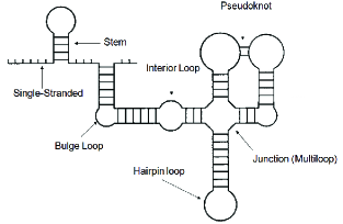
The word hairpin refers to a structure or substructure, whose faces are consecutive region of stacking regions, bulges and interior loops, ending with a hairpin loop [1].

1.3 The software

The software’s main tasks are to re-generate the structure from the output that represents the hydrogen bond, to analyse it and to compare it with another structure of similar sequence. The software is suited for the output of the Vienna package in which a matched pair is represented by parentheses (example is presented in Figure 2), and can be easily adopted to suit the output that presents the paired bases, which is also common. It was programmed in c++ in Unix environment (Unix compiler), using Eclipse.

1.4 Generation of the secondary structure

The software uses tree representation (example is presented in Figure 2) for the structures, which is used for secondary structures and assumes no psuedo-knots. The software divides the structure into substructures, which include a sequence of faces with 2 interior edges and a hairpin loop or a multiloop as their last face. Each substructure may contain sons, which are substructures, that are connected to it via a multiloop. In the case of a multiloop, it contains the first pair of the multiloop, and the sons contain as their first pair the other pairs of the multiloop.

Figure 2: An example of a secondary structure $\left(a\right)$ and its parenthesis $\left(b\right)$ and tree representations $\left(c\right)$

$\left(a\right)$

$\left(b\right)$

(((….))).((((((…))(((..))))))).

$\left(c\right)$

structure

$\swarrow\searrow$

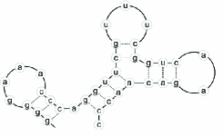
structure  hairpin structure

$\swarrow\,\,\,\,\,\,\,\,\searrow$

hairpin structure hairpin structure

In the process of identifying the tree representation the faces are detected, classified and stored in each sub-structure (the pairs are also stored in a different list). It is here to mention that the software also stores in each face the unbound nucleotides. A detailed description of the algorithm is given in Appendix 3.1.

• The functionality of the software in generating structures was verified on five RNA outputs.

1.5 Structure comparison

In order to compare two structures of the same RNA, the faces were compared. They were divided into three groups: identical, meaning that they have the same structure, nucleotide sequences and nucleotide indexes. Similar, meaning that they have the same structure, nucleotide sequence and not the same nucleotide indexes. And different, meaning that it doesn’t fall into the two categories mentioned (A detailed description of the algorithm is given in Appendix 3.2). This division enables us, in case of different structures, to identify the list of faces that have different free energy values. Thus, faces which are suspected of having incorrect energy values may be focused on. The functionality of this comparison was checked on the structures of the RNAs: PDB_00030, PDB_00213, PDB_00394 and yielded the expected results.

1.6 Applications

The main uses of the structural analysis can be the following:

• Comparison between structures of minimum free energy, found by different algorithms, and thus trying to extract in which cases they yield different results. It can be used to compare the mfe (minimum free energy) structures predicted by the Vienna package and by other algorithms that have different free energy parameters. When the structures are different, the software can output the faces predicted by both and the origin of the difference can be estimated.

• Comparison between structures of minimum free energy of a certain algorithm and the experimental results. One can assess which are the cases where differences exist. Here again, the origin of difference can be identified and the parameters of the algorithm can be corrected accordingly.

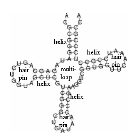
• Identification of structural motives (found by analyzing the structures predicted by the algorithms) that are common in a group of RNAs, which may lead to classification and possible functionality. It can be also used to associate RNA to a group of RNAs once its structural motives are known. An example for such structural similarity is the family of tRNA that includes a helix, which leads to a multiloop which is followed by three helices that end with an hairpin loop (typical secondary structure of tRNA is shown in Fig 3). A possible application, can be the PASRs (promoter associated small RNAs) that are transcribed from the promoter’s regions. These PASRs bind at the promoter, and reduce the expression of the associated gene. The secondary structure of PASRs can be predicted using existing software. Then, using this software, structural motives that are common can be detected and a structural possible classification, and even a functional mechanism can be estimated [2].

Figure 3: Typical secondary structure of tRNA

• Identification of certain sequences that are repeated in a group of RNAs, especially in unpaired nucleotides, which may provide clues about their function (can be done using experimental or predicted secondary structures). An example of repeated sequences is the selenoprotein mRNA sequences. These mRNAs include the UGA codon which has a dual function. It signals both the termination of protein synthesis and incorporation of the amino acid selenocysteine. Decoding of selenoprotein translation requires the SECIS element, a stem-loop motif in the 3’-UTR of the mRNA, carrying short or large apical loop. SECIS elements contain an Adenosine that precedes the quartet of non–Watson-Crick base pairs, a UGA_GA motif in the quartet, and two adenosines in the apical loop or bulge [3][4].

1.7 Initial results

The following RNA sequences: PDB 30,32,45,213,394,547,584,750,1236 were compared (experimental structures versus Vienna package results) to get initial results for the differences between the structures.

It seems that two of the main sources of difference between the experimental structures and the ones predicted by the algorithm were the following:

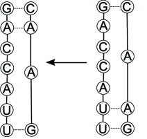
• Bonds that appeared in the experimental structures and weren’t allowed by the algorithms (Vienna package and others), like A-A U-C G-A G-G.

• Hairpin Loops, containing less than 4 exterior edges (3 in the tested sequences) were included in the experimental structures and aren’t allowed by the algorithms.

It was seen that in some cases (PDB 32,213,394,547,750,1236), the differences were local, meaning that there were identical faces in a substructure, then different faces, and then an identical pair which terminates the local region of difference.

Looking in the literature about the pairs which were detected in the experimental structures checked, and weren’t allowed by the algorithms, it seems that these pairs also show up in other cases in RNA structures. Such an example is G-A/A-G pairing found in SECIS element in the 3’ untranslated region of Se-protein mRNA and in the functional site of the hammerhead ribozyme. The measured melting temperature values of RNA oligonucleotides having this pair showed an intermediate value, between that of the Watson-Crick base pairs and that of non-base pairs [5][6]. Although rare, A-A and G-G pairs also occur in some cases. It was seen that a single G-G pair has a stabilizing effect and can stabilize an internal loop [7] and that a group of Adenine bases can have interactions with each other in a bulge [8]. Another study shows that the water-mediated UC pair is a structurally autonomous building block of the RNA [9]. Thus it seems that the structure of the RNA may be affected also by interactions that are less dominant.

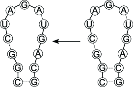
The tetraloops (Hairpin Loops, containing 3 exterior edges) that were seen in the experimental data, seem to belong to the three types of tetraloops that are common in RNA: GNRA,UNCG and CUUG (R=purine, N=every nucleotide). Meaning that the algorithms exclude these types of faces although if formed they may lead to a lower total free energy.

Since the total number of different faces may be large, it is possible to detect regions of difference and output local differences. Thus differences containing smaller number of faces can be detected, and tendencies may be pointed out. It can be done by detecting a sequence of identical faces followed by a sequence of different faces that ends with an identical pair. Similar faces that belong to that region can also be detected, and the number of different faces can be further reduced.

The local differences that were found are the following: (it should be noted here that the solid and dashed lines represent covalent and hydrogen bonds respectively and that the arrows point to the experimental data)

Figure 4: local differences for PDB 32

Experimental structure   Vienna package prediction

(a)

(b)

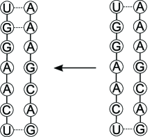
(c) Hairpin loop

Figure 5: local differences for PDB 213

Experimental structure   Vienna package prediction

(a)

(b)

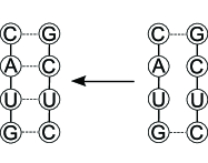
(c) Hairpin loop

(d) Hairpin loop

(e)

Figure 6: local differences for PDB 394

Experimental structure   Vienna package prediction

(a) Hairpin loop

(b) Multiloop

1.8 Discussion

It can be concluded that the energy parameters of the algorithms give good predictions for the structures, and in most cases the general structure is well predicted. However, if we assume that the total free energy of a structure is the sum of the free energies of the faces, there are still faces whose free energy parameters aren’t estimated well enough. Local differences may lead to more specific cases of mismatch, and thus help us focus on the faces that still have to be investigated.

Certain differences between the structure of PDB 394 found experimentally and the one predicted by the Vienna package may suggest that the free energy of a multiloop may vary significantly by its extension by 2 nucleotides. (the multiloop was extended rather than form a G-C hydrogen bond as suggested by the Vienna package). This may be due to the entropic loss caused by its reduction by two nucleotides.

Since the differences mainly originate from faces and hydrogen bonds that are not allowed by the Vienna package it is suggested that prediction may be improved by integrating parameters of these faces into the software and predicting unallowed hydrogen bonds according to the relevant face respectively. This may lead to a more accurate and detailed description of the pairs in the secondary structure prediction.

2 Calculation of free energy of an interior loop

2.1 Introduction

In the last decade, RNA has gained much attention, due the discovery that it fulfills a considerable diversity of biological tasks, including enzymatic and regulatory functions. Since RNA structure is highly related to its functionality, its of a top priority to predict and analyse secondary and tertiary RNA structures.

The most common software that predict secondary structure are the Vienna package/Mfold . These software assume that the total free energy of a secondary structure is the sum of the free energies of its faces (planar regions, bounded on all sides by covalent or hydrogen bonds between nucleotides) [1]. These free energy parameters are extracted from experiments in which initial concentrations of reactors that are RNA segments are changed, and the melting temperature for the reaction is measured (read Appendix 3.3.1 for more details). However, in most of these experiments the heat capacity was assumed not to depend on the temperature, so they are to be redone (read Appendix 3.3.2 for more details). Here, we try to check the feasibility of a numerical calculation of the free energy values of faces, using a Monte-Carlo simulation. In the case that such a calculation will be feasible, it might provide an alternative to the experiments that are done, and supply more specific information, since in the experiments the faces’ free energy values are derived by fitting measured values of the larger secondary structures in which they are included.

This work is also relevant for calculation of thermodynamic properties of a complete RNA sequence and its tertiary free energy landscape, as it can be easily adopted to do so (assuming no pseudoknots). This is of importance due to the relatively small number of theoretical works on RNAs as compared to the vast number of studies on proteins. These theoretical works on RNAs are composed of mostly MD simulations in which a definition of the coordinate of interest is introduced in advance, in order to investigate the free energy landscape. There are relatively fewer Monte-Carlo simulations that involve the calculation of thermodynamic properties.

In this work we present how the information gathered in a parallel tempering procedure (details are in 2.4) can be used to calculate the free energy differences. In this calculation we had to reach equality of partition functions and since we didn’t want to be restricted to systems that have the same high temperature description, we had to go into imaginary regimes in which the steric constraints were relaxed. This regime was reached due to the use of cutoff energy which is also relevant to sampling problems that appear in the Thermodynamic Integration method [10][11][12].

2.2 Goals

The goals of this project are the following:

• Model the RNA and the different interactions between the sites.

• Perform Monte-Carlo simulation in which the space of states will be sampled correctly, and that will converge and be consistent.

• Writing a software that will run in reasonable time frames.

• Calculation of free energy of internal loops that can, in a more elaborate model, generate the free energy values used in the Vienna package.

2.3 The Model

In this project, we modeled and simulated an interior loop composed of 6 nucleotides - 3 in each strand. In this type of interior loop the first and last pair are bound in canonical or wobble base pairing, and the pair in the middle can have in the general case all combinations of bases, not belonging to the canonical or wobble base pairings. Specifically in this project we chose to simulate the following interior loop:

Figure 7: Simulated Interior loop

where X stands for all types of nucleotides (A,C,G,U).

2.3.1 Semi-coarse grained model of an Interior loop of RNA

The model is partly coarse grained and partly in full atomistic detail. It is coarse-grained in its backbone description and in full atomistic detail in the description of the nucleobases. This choice of modelling of the structure is due to the important role the bases play in the interactions, as the base pairing and the stacking energies are the dominant ones.

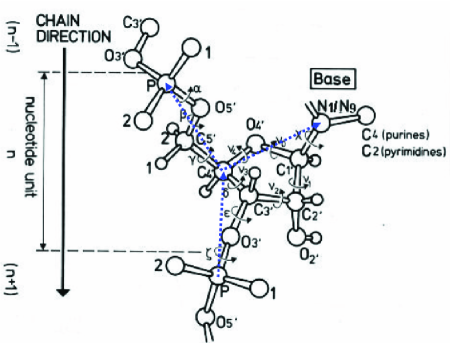
The model reduces the complexity of the backbone to two point interaction sites, one for the phosphate and one for the starting point of the ribose. The phosphate interaction site was chosen to reside where the P atom is located (all relevant atoms are presented in fig 8), and the (beginning of the) ribose interaction site was chosen to reside where the C4’ atom is located. Reasoning for this choice is the fact that the torsion angles about the two C-O bonds, are preferably in the trans rotational isomeric state [13], which means that the P-C4’ and C4’-P bond lengths don’t vary much. It should be noted that according to the location of the C4’ and P atoms, the building of the RNA backbone in atomic detail [14] and as a result the ribose can be achieved (The torsion angle $\delta$ determines the configuration of the ribose [15]).The bases were assumed to be rigid planar objects as implied by [16]. The modelling of the bases included all the atoms (see Fig. 9 for details), what enables them to form Watson-Crick, and Hoogsteen base pairing [17]. The atoms’ coordinates were calculated in the system of coordinates whose two base vectors reside in the bases’ plane (based on the data form [18]). The bases were assumed to be connected to the C4’ atom from the N1 atom in purines and the N9 in pyrimidines. The distances between the two backbone sites, as well as the distance between the C4’ atom and the N1/N9 atom were chosen to be fixed. This was supported by an analysis of PDB files performed in which they showed small standard deviations (it was also reported in [19] that the backbone bonds defined have lengths of $\sim 3.9\overset{\circ}{A}$). The distances between the interaction sites were chosen to be the ones found in a specific pdb file (1AFX.pdb), for simplicity. It has to be mentioned here, that this modelling of the interior loop doesn’t necessarily have less degrees of freedom than a full atomistic model. However, the treatment in terms of programming time is shorter.

For an interior loop, there are two pairs of canonical/wobble hydrogen bonds. The pairing is between the first base in one strand and the last base in the second strand, and between the last base in one strand and the first base in the second strand. In the model, it was assumed that the orientation of the paired bases is constant with respect to each other. Regarding the other bases, they were assumed to have freedom of movement - the C4’-N bond was free to rotate and the base was free to rotate with respect to this bond. All the interaction sites in the backbone were also free to move with the restrictions that the first pair of bases is constant in space (due to rotation and translation symmetry), and the last pair of bases is treated like a rigid object (assumed to have fixed pairing geometry) and free to move.

Figure 8: Atomic numbering scheme and definition of torsion angles

Figure 9: The four bases and their atoms

A                                U

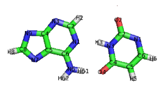
G                                C

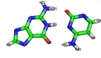
2.3.2 The energy model

The following energy terms were considered in the model:

2.3.2.1 Stacking energy

One of the dominant terms is the stacking energy between the bases, which originates from dispersive and repulsive interactions. The stacking energy is calculated between all the atoms in the bases and is represented by the 6-12 Lennard Jones potential:

$$\mathcal{H}_{\mathrm{stacking}}=\underset{\underset{\alpha\neq\beta}{\alpha,\beta}}{\sum}\underset{i,j}{\sum}\epsilon_{ij}\left[\left(\frac{r_{m_{r_{i\left(\alpha\right)j\left(\beta\right)}}}}{r_{i\left(\alpha\right)j\left(\beta\right)}}\right)^{12}-2\left(\frac{r_{m_{r_{i\left(\alpha\right)j\left(\beta\right)}}}}{r_{i\left(\alpha\right)j\left(\beta\right)}}\right)^{6}\right]$$ (1)

where $r_{i\left(\alpha\right)j\left(\beta\right)}$ and $r_{m_{r_{i\left(\alpha\right)j\left(\beta\right)}}}$ are the distance between atoms and the distance at which the energy is minimum respectively ($i\left(\alpha\right)$ is atom $i$ of base $\alpha$).

It can be easily seen that the minimum energy is $\epsilon$ and that we get infinite energy at $r\rightarrow 0$ and zero energy at $r\rightarrow\infty$.

The distances of minimum energy were chosen from [20] and the energy values were chosen from [21] in order to be consistent with behavior of bases as reported in [22].

The dominant energy terms have distance of minimum energy in the range $3\overset{\circ}{A}<r_{m_{ij}}<3.4\overset{\circ}{A}$ and minimum energies in the range $0.15\frac{KCal}{Mole}<\epsilon_{ij}<0.2\frac{KCal}{Mole}$

2.3.2.2 Base-pairing energy

Another dominating term is the base-pairing energy that originate mainly from the hydrogen bonds.

The potential is much more localized and was chosen to be:

$$\mathcal{H}_{\mathrm{bp}}=\underset{i,j}{\sum}h_{bp_{ij}}T_{ij}\,\,\,\,\,\,\,$$ (2)

where

$$h_{\mathrm{bp_{ij}}}=\varepsilon_{ij}\left[\left(\frac{r_{m_{ij}}}{r_{ij}}\right)^{12}+tgh\left(31\left(\frac{r_{ij}-2}{r_{m_{ij}}}\right)\right)-1-0.8\left(\frac{r_{m_{ij}}}{r_{ij}}\right)^{6}\right]$$ (3)

and

$$T_{ij=}\left\{\begin{array}[]{cc}cos^{2}\theta_{ij}&h_{\mathrm{bp}}<0\\ 1&h_{\mathrm{bp}}\geq 0\end{array}\right.$$ (4)

$\theta_{ij}$ is the angle between the acceptor atom, the polar hydrogen and the donor atom (see Fig 10), and

$i,j$ are the indexes of the hydrogen and the acceptor respectively.

The term $tgh\left(31\left(\frac{r_{ij}-2}{r_{m_{ij}}}\right)\right)-1$ was introduced to achieve locality in the potential (keeping the energy zero at infinity), and the term $cos^{2}\theta$ was introduced to achieve directionality.

Figure 10: The angle between the acceptor atom, the polar hydrogen and the donor atom

The distance of min. energy is $r_{m_{ij}}=1.9\overset{\circ}{A}$ and the min. energies values $\varepsilon_{ij}$ are chosen according to the acceptor and the electronegativity of the donor. Explicitly, $\varepsilon_{ij}$ is the product of the difference in electronegativity between the hydrogen atom and the donor, and a factor that accounts for the effect of the number of the lone pairs of the acceptor - 1 for N and 2 for O (electrons in the outer shell can participate in the interaction).

Another proposed potential is with:

$$T_{ij=}\left\{\begin{array}[]{cc}cos^{4}\theta_{ij}&h_{\mathrm{bp}}<0\\ 1&h_{\mathrm{bp}}\geq 0\end{array}\right.$$ (5)

and with the factor that accounts for the effect of the number of the lone pairs of the acceptor - 1 for N and 1.15 for O. This choice is pretty much in accordance with the energy parameters in [23].

2.3.2.3 Electrical energy

Coulombic interactions are taken into account using the Debye-Huckel approximation, which is valid for the low-salt physiological conditions.

The Coulombic interactions in the model are between the oxygens next to the phosphates, and are calculated between phosphates of consecutive nucleotides (as in [24]).

$$V_{qq}=\underset{i<j}{\overset{N}{\sum}}\frac{q_{i}q_{j}}{4\pi\varepsilon_{o}\varepsilon_{k}r_{ij}}e^{-r_{ij}/\kappa_{D}}$$ (6)

where

$$\kappa_{D}=\sqrt{\frac{\varepsilon_{0}\varepsilon_{k}RT}{2N_{A}^{2}e_{q}^{2}I}}$$ (7)

and $I$ is the ionic strength. We used [Na+]=50mM ($\kappa_{D}=13.6\overset{\circ}{A}$).

(according to the physiological conditions [Na+]=150mM [Mg++]=12mM ($\kappa_{D}=6.835\overset{\circ}{A}$) )

2.3.2.4 Excluded volume interaction

The excluded volume terms were introduced in order to obey steric constraints. They are calculated between all atoms and sites, taking into account the combinations which aren’t included in the stacking energy and in the base-pairing calculations.

The interaction used is identical to the stacking, shifted up, and with a cutoff radius above which on this energy is zero.

The term is the following:

$$H_{\mathrm{excluded\,volume_{ij}}}=\left\{\begin{array}[]{cc}\epsilon_{ij}\left[\left(\frac{r_{cutoff}}{r_{ij}}\right)^{12}-2\left(\frac{r_{cutoff}}{r_{ij}}\right)^{6}+1\right]&r<r_{cutoff}\\ 0&r\geq r_{cutoff}\end{array}\right.$$ (8)

where we chose $r_{cutoff}=r_{m_{ij}}$.

In the following figure the typical energies as a function of distance are presented:

Figure 11: Typical energies as a function of distance

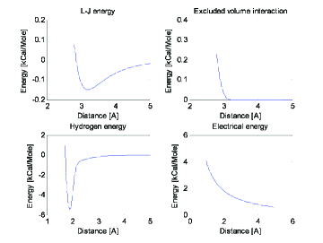
2.4 The Monte-Carlo Simulation and parallel tempering

In order to to simulate the behavior of the system, the Monte-Carlo method was used.

It was used with the Metropolis Criterion, according to which a new configuration is accepted with probability of

$$P_{i\rightarrow j}=min\left\{1,e^{-\beta\left(H_{i}-H_{j}\right)}\right\}$$ (9)

Since the Metropolis Criterion satisfies the detailed balance condition  (see Appendix 3.4 for details)

$$P_{i}P_{i\rightarrow j}=P_{j}P_{j\rightarrow i},$$ (10)

all suggested moves were chosen such that a move and its reverse have the same a-priori probability.

In order to sample all possible states with the model’s restrictions, the following MC moves were used:

1. External move - a crankshaft move of the backbone. In this move two sites of the backbone are randomly chosen, and all the sites between them are rotated by a random angle with respect to the axis that connects the two chosen sites. The rotation angle was generated according to a normal distribution with a standard deviation of 7^∘.

2. Internal move - random selection of an unpaired nucleotide. Then, a random selection between the following moves:

• Random rotation of the base with respect to a random vector with N1/N9 held fixed.

• Random rotation of the C4’-N1/9 vector (bond) and the base, with respect to a random vector, with C4’ held fixed.

The rotation angles for both internal moves were generated using normal distribution with a standard deviation of 5^∘.

In order to generate random vectors, $\theta$ was generated with the distribution of

$$f\left(\theta\right)=\frac{sin\theta}{2}\,,\theta=\left[0,\pi\right]$$ (11)

and $\phi$ was generated with a uniform distribution

$$f\left(\phi\right)=\frac{1}{2\pi},\,\phi=\left[0,2\pi\right]$$ (12)

Thus, the locations on the unit sphere/the solid angles were generated with a uniform distribution

$$f\left(\Omega\right)=\frac{1}{4\pi},\,\Omega=\left[0,4\pi\right]$$ (13)

In each move, after the locations of the sites are updated, the bond and torsion angles are calculated (according to [25]).

In order to sample the states of configurations correctly during the simulation without being trapped in local minima, parallel tempering has been used [26].

The general idea of parallel tempering is to simulate M replicas of the original system of interest, each replica at a different temperature. The high temperature systems are generally able to sample large volumes of phase space, whereas low temperatures systems, whilst having precise sampling in a local region of phase space, may become trapped in local energy minima during the timescale of a typical simulation. Parallel tempering achieves good sampling by allowing the systems at different (usually adjacent) temperatures to exchange complete configurations. Thus, the inclusion of higher temperatures ensures that the lower temperature systems can access a representative set of low temperature regions of phase space. The M systems can be considered as one artificial system that contains M non-interacting replicas. We can define the state of the artificial system as $\mathcal{C}=\left\{C_{1},C_{2},...,C_{M}\right\}$, where $C_{i}$ is the state of replica $i$ with energy $H_{i}=H\left(C_{i}\right)$ . It can then be seen, that the probability of switching adjacent configurations according to the Metropolis criterion is

$$P\left(\mathcal{C}\rightarrow\mathcal{C}^{\prime}\right)=min\left\{1,\frac{e^{-\beta_{i}H_{i+1}-\beta_{i+1}H_{i}}}{e^{-\beta_{i}H_{i}-\beta_{i+1}H_{i+1}}}\right\}=min\left\{1,e^{+\left(\beta_{i+1}-\beta_{i}\right)\left(H_{i+1}-H_{i}\right)}\right\}=min\left\{1,e^{\Delta}\right\}$$ (14)

To ensure that an exchange of the conformation between two copies will happen with sufficient probability, $\Delta$ has to be on the order of one. If we approximate $H_{i}$ as the average energy of system $i$, we can write:

$$\Delta\approx\left(\triangle\beta\right)^{2}\frac{\partial U}{\partial\beta}$$ (15)

where $\Delta\beta=\beta_{i+1}-\beta_{i}$

Since the average energy grows roughly linearly with the number of residues $N$, $\Delta\beta$ should be of the order of $\frac{1}{\sqrt{N}}$ [27].

In our case $N\approx 70$, so we need approximately 8-9 different temperatures, that have to be spread up to a temperature at which the dominating interactions will have a mild effect on the system’s behavior.

2.4.1 Ratios between the different MC moves

• For each external move, 90 internal moves are performed.

• For each configuration exchange attempt, 10 external moves are performed.

2.5 Parallel tempering and the calculation of free energy differences

2.5.1 Introduction

Our goal is to find the free energy difference between two systems: two interior loops, which differ in a base. Specifically we will calculate the free energy difference between the interior loops $\tilde{G}$, whose second base is G, and $\tilde{C}$, with the base C, as shown in Fig 12.

Figure 12: $\tilde{C}$ and $\tilde{G}$

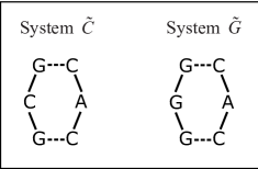
We denote this difference by $\triangle F_{\tilde{C}\rightarrow\tilde{G}}\left(\beta_{1}\right)=F_{\tilde{G}}(\beta_{1})-F_{\tilde{C}}(\beta_{1})$.

The state of the bases $G,C$ (the coordinates of all their atoms) for a given location of the N1/N9 atom of the base (see Fig 9 for details) is determined by three angles, since the bases are assumed to be rigid planar objects. Therefore the same degrees of freedom are associated with these different bases, and since the two systems $\tilde{G},\tilde{C}$ differ just in the bases, the two systems have the same degrees of freedom.

The difference of free energy between any two systems that have the same degrees of freedom can, in principle, be calculated by the Thermodynamic Integration (ThI) method, as described in section 2.5.2. ThI requires running simulations of different instances (several values of a parameter $\lambda_{i},i=1,2,...m$) of a hybrid $\tilde{G}-\tilde{C}$ system.

These systems have a rugged energy landscape (with many local minima), which means that the decorrelation time in a “naive” Monte-Carlo simulation are exponentially long. One of the widely used methods to alleviate the problem of equilibrating systems with such landscapes is parallel tempering (PT), which we describe below in Section 2.5.3. PT involves simulating the system of interest, in parallel, at several (inverse) temperatures $\beta_{i},i=1,2,...n$.

The natural way to calculate the free energy difference for our two systems, $\triangle F_{\tilde{C}\rightarrow\tilde{G}}\left(\beta_{1}\right)$ is, therefore, by ThI, equilibrating $m$ systems, one for each value of $\lambda_{i}$. For each such equilibration PT is used, at $n$ temperatures, hence all together $nm$ systems are simulated. In section 2.5.4 we describe a method, Temperature Integration (TeI), which allows us to calculate the free energy difference much more efficiently than the use of ThI with parallel tempering.

2.5.2 Thermodynamic Integration

Thermodynamic Integration (ThI) is one of the most commonly used methods for calculating the free energy difference between two systems. It is described in detail in Appendix 3.5. This method is used to calculate the free energy difference between two systems with the same degrees of freedom [12, 10, 11], by varying a parameter $\lambda$ that interpolates between the two compared systems. We will use the systems $\tilde{C}$ and $\tilde{G}$ described above to demonstrate application of this general method in a specific context.

Denote the Hamiltonians of the two systems by $H_{\tilde{C}}(\mathbf{\boldsymbol{\theta}})$ and $H_{\tilde{G}}(\mathbf{\boldsymbol{\theta}})$, where $\mathbf{\boldsymbol{\theta}}$ denotes the coordinates of the system. Noting that the two systems have the same coordinate space, we define a $\lambda$ - weighted hybrid system, characterized by the Hamiltonian $H(\lambda):$

$$H(\lambda,\mathbf{\boldsymbol{\theta}})=\lambda H_{\tilde{G}}(\mathbf{\boldsymbol{\theta}})+(1-\lambda)H_{\tilde{C}}(\mathbf{\boldsymbol{\theta}})$$ (16)

As shown in Appendix 3.5, the free energy difference is given by

$$\triangle F_{\tilde{C}\rightarrow\tilde{G}}\left(\beta_{1}\right)=\intop_{0}^{1}\left[\left\langle H_{\tilde{G}}(\mathbf{\boldsymbol{\theta}})\right\rangle_{\lambda}-\left\langle H_{\tilde{C}}(\mathbf{\boldsymbol{\theta}})\right\rangle_{\lambda}\right]d\lambda$$ (17)

where $\left\langle X\right\rangle_{\lambda}$ denotes the equilibrium average of $X$ in the ensemble characterized by $H(\lambda)$. The expression for $\triangle F_{\tilde{C}\rightarrow\tilde{G}}\left(\beta_{1}\right)$, written explicitly, takes the form:

$$\triangle F_{\tilde{C}\rightarrow\tilde{G}}\left(\beta_{1}\right)=\intop_{0}^{1}\left\{\int\left[H_{\tilde{G}}(\mathbf{\boldsymbol{\theta}})-H_{\tilde{C}}(\mathbf{\boldsymbol{\theta}})\right]\frac{e^{-\beta_{1}\left[\lambda H_{\tilde{G}}(\mathbf{\boldsymbol{\theta}})+\left(1-\lambda\right)H_{\tilde{C}}(\mathbf{\boldsymbol{\theta}})\right]}d\mathbf{\boldsymbol{\theta}}}{Z(\lambda)}\right\}d\lambda$$ (18)

with

$$Z(\lambda)=\int e^{-\beta_{1}\left[\lambda H_{\tilde{G}}(\mathbf{\boldsymbol{\theta}})+\left(1-\lambda\right)H_{\tilde{C}}(\mathbf{\boldsymbol{\theta}})\right]}d\mathbf{\boldsymbol{\theta}}$$ (19)

The integration is performed numerically, with the integrand evaluated at each one of a set of values of $\lambda$ by Monte Carlo simulations. As implied by (18), the two systems are required to have the same degrees of freedom.

2.5.3 Thermodynamic integration with parallel tempering

The systems $\tilde{C}$ and $\tilde{G}$, and the $\lambda$-weighted system have rugged energy landscapes with many local minima. As the decorrelation times grow exponentially with $\triangle E/kT$ , where $\triangle E$ is the energy barrier between nearby valleys, equilibration times in these systems can be rather long. In order to overcome this problem, and obtain the thermodynamic averages $\left\langle H(\theta)\right\rangle_{\lambda}$, one can use the Parallel Tempering procedure [26, 27]. However, implementing both thermodynamic integration and parallel tempering yields an unnecessary overhead in running time, as we will demonstrate.

In order to implement thermodynamic integration we first choose a set of values $\lambda_{i},\leavevmode\nobreak\ i=1,...m$, that will enable us to have a good sampling of the function $\left\langle H(\mathbf{\boldsymbol{\theta}})\right\rangle_{\lambda}$ for the integration in eq. (17). Thus, $m$ is related to the desired precision of the integration.

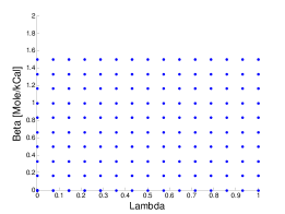
In principle parallel tempering should be performed for each $\lambda_{i}$, simulating each of the $m$ $\lambda_{i}$ weighted systems over a set of temperatures, given by $\beta_{j},\leavevmode\nobreak\ j=1,...n$. Finally, using the calculated values of $\left\langle H(\mathbf{\boldsymbol{\theta}})\right\rangle_{\lambda_{i}}$ at a temperature of interest $\beta_{1}$, we approximate the integral of eq. (17) by a sum over $m$ terms, to get the free energy difference $\triangle F_{\tilde{C}\rightarrow\tilde{G}}\left(\beta_{1}\right)$.

The procedure involves running Monte-Carlo simulations over $m$ $\lambda$-values, and $n$ $\beta$-values, that is, over a grid of $m\times n$ instances of the hybrid system. An illustration of this grid is presented in figure 13.

Figure 13: Illustration of the grid of values over which the Monte-Carlo simulations are performed. The lowest values of $\beta$ correspond to some very high finite temperature.

2.5.4 Calculation of $\Delta F$ by parallel tempering

We present now a method which uses only simulations obtained in the process of parallel tempering (skipping the need for simulations at a set of $\lambda_{i}$ values), performed for the two systems $\tilde{C}$ and $\tilde{G}$, to obtain the free energy difference $\triangle F_{\tilde{C}\rightarrow\tilde{G}}\left(\beta_{1}\right)$. This method can be applied to any two systems that have the same degrees of freedom $\boldsymbol{\theta}$.

As $\beta\to 0$, the limiting value of the partition function of a system yields the phase space volume. In particular, if systems $\tilde{C}$ and $\tilde{G}$, which have the same coordinate space $\boldsymbol{\left\{\theta\right\}}$, have the same $\beta\to 0$ limit, we have

$$Z_{\tilde{G}}\left(\beta\to 0\right)=Z_{\tilde{C}}\left(\beta\to 0\right)=\int d\boldsymbol{\theta}\,.$$ (20)

In this case we can use the following identity to obtain, for a finite $\beta_{1}$, the difference of the free energies:

$$\ln Z\left(\beta_{1}\right)-\ln Z\left(\beta\to 0\right)=\int_{0}^{\beta_{1}}\frac{d\ln Z}{d\beta}d\beta=-\int_{0}^{\beta_{1}}\left\langle H\right\rangle d\beta\,.$$ (21)

Using equations (20) and (21) we obtain

$$\triangle F_{\tilde{C}\rightarrow\tilde{G}}\left(\beta_{1}\right) = \frac{1}{\beta_{1}}\left[\ln Z_{\tilde{C}}\left(\beta_{1}\right)-\ln Z_{\tilde{G}}\left(\beta_{1}\right)\right]$$ (22)

$$= \frac{1}{\beta_{1}}\left[\intop_{0}^{\beta_{1}}\left\langle H_{\tilde{G}}\right\rangle d\beta-\intop_{0}^{\beta_{1}}\left\langle H_{\tilde{C}}\right\rangle d\beta\right]\,.$$

For each of the systems $\tilde{C}$ and $\tilde{G}$ we estimate the integrals on the right hand side by parallel tempering, sampling the system at a series of values $\beta_{1},\ldots,\beta_{n}$. We choose values such that $\beta_{n}^{-1}$ is much larger than the internal energy of the system at $\beta_{1}$, so $Z(\beta_{n})\cong Z(\beta\to 0)$.

The condition of eq. (20) poses a problem for the particular systems $\tilde{C}$ and $\tilde{G}$ studied here. The steric excluded volume interactions are not bound in our model, and hence, the available phase space volumes for the two systems are not equal at any temperature, and equation (20) does not hold. In order to satisfy the condition stated above we had to set a cutoff over the steric interactions, $E_{\mathrm{cutoff}}$. In the next section we show that our results do not depend on the choice of $E_{\mathrm{cutoff}}$ and $\beta_{n}$, as long as $E_{\mathrm{cutoff}}$ is much larger than any typical interaction energy in the system at $\beta_{1}$, and $\beta_{n}^{-1}\gg E_{\mathrm{cutoff}}$.

2.5.5 Passing the steric energy barriers by introducing a cutoff energy

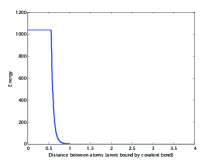
We now tackle the problem of sampling at temperatures which are higher than all energy terms, by using a cutoff energy in the steric interaction potential. We denote the cutoff energy and the distance from which the energy will be set to the cutoff energy by $E_{\mathrm{cutoff}}$ and $r_{\mathrm{cutoff}}$ respectively.

The modified steric potential can be written as follows:

$\left(\frac{\sigma}{r}\right)^{12}\rightarrow H_{\mathrm{steric}}\left(r\right)=\left\{\begin{array}[]{cc}\left(\frac{\sigma}{r}\right)^{12}&r>r_{\mathrm{cutoff}}\\ E_{\mathrm{cutoff}}&r\leq r_{\mathrm{cutoff}}\end{array}\right.$

In the following figure an example of such a steric potential is presented:

Figure 14: Plot of an example of a steric interaction potential that includes a cutoff energy

The proposed calculation of the free energy difference between the two systems at the temperature of interest $\beta_{1}$ is legitimate only if our choice of the cutoff energy has a negligible effect on the partition function of each of the two systems at $\beta_{1}$. In addition, the highest temperature used, $\beta_{2}$, must be such that the equality of the partition functions of the two systems is satisfied to a good accuracy.

We denote the Hamiltonian with the cutoff energy by $H^{\prime}$, and write the requirements stated above explicitly as follows:

$$lnZ_{\tilde{G}}\left(\beta_{1},H\right)\simeq lnZ_{\tilde{G}}\left(\beta_{1},H^{\prime}\right)$$ (23)

$$lnZ_{\tilde{C}}\left(\beta_{1},H\right)\simeq lnZ_{\tilde{C}}\left(\beta_{1},H^{\prime}\right)$$ (24)

$$lnZ_{\tilde{G}}\left(\beta_{2},H^{\prime}\right)\simeq lnZ_{\tilde{C}}\left(\beta_{2},H^{\prime}\right)$$ (25)

In order for the cutoff to have a negligible effect on the partition functions at the temperature of interest it has to be set to a value that satisfies $E_{\mathrm{cut\,off}}\gg kT_{1}$.

As for $\beta_{2}$, if the cutoff energy satisfies $E_{\mathrm{cut\,off}}\ll kT_{2}$, the systems will have almost equal probability to be in all the regions of their phase space, including ones in which the molecules entered the “volume” of one another. Thus, the partition functions of the two systems will be almost equal.

Hence if these requirements are satisfied one can write:

$$lnZ_{\tilde{C}}\left(\beta_{1},H\right)-lnZ_{\tilde{G}}\left(\beta_{1},H\right)\simeq$$ (26)

$$lnZ_{\tilde{C}}\left(\beta_{1},H^{\prime}\right)-lnZ_{\tilde{G}}\left(\beta_{1},H^{\prime}\right)\simeq$$ (27)

$$lnZ_{\tilde{G}}\left(\beta_{2},H^{\prime}\right)-lnZ_{\tilde{G}}\left(\beta_{1},H^{\prime}\right)-\left[lnZ_{\tilde{C}}\left(\beta_{2},H^{\prime}\right)-lnZ_{\tilde{C}}\left(\beta_{1},H^{\prime}\right)\right]$$ (28)

Using the identity in eq (21), we can write:

$$\triangle F_{C\rightarrow G}\left(\beta_{1},H\right)=\frac{1}{\beta_{1}}\left[lnZ_{\tilde{C}}\left(\beta_{1},H\right)-lnZ_{\tilde{G}}\left(\beta_{1},H\right)\right]\simeq\frac{1}{\beta_{1}}\left[\intop_{\beta_{2}}^{\beta_{1}}\left\langle H^{\prime}_{G}\right\rangle d\tilde{\beta}-\intop_{\beta_{2}}^{\beta_{1}}\left\langle H^{\prime}_{C}\right\rangle d\tilde{\beta}\right]$$ (29)

So the calculation of free energy will be negligibly affected by the use of a cutoff energy as long as we fulfill the relevant conditions.

It has to be mentioned that this use of cutoff energy is relevant also to ThI and similar methods. In these methods if the systems have different $\beta\to 0$ limit, at $\lambda=0,1$ due to the steric energy terms (represented by $\left(\frac{\sigma}{r}\right)^{12}$) micro-states may have infinite energy. As a result the internal energy will be infinite and the sampling of the internal energy will be infeasible.

It can be seen that since the free energy difference between systems that have the Hamiltonian with the cutoff $H^{\prime}$ is almost equal to the one calculated between systems with the Hamiltonian $H$

$\triangle F_{C\rightarrow G}\left(\beta_{1},H\right)\simeq\frac{1}{\beta_{1}}\left[lnZ_{\tilde{C}}\left(\beta_{1},H^{\prime}\right)-lnZ_{\tilde{G}}\left(\beta_{1},H^{\prime}\right)\right],$

ThI can be derived for systems with $H^{\prime}$ and yield almost the same result.

In conclusion, with the use of cutoff energy in ThI, that enables us to sample the integrand in all cases, the free energy difference between any two systems that have the same degrees of freedom can be calculated.

• Cutoff energies chosen for the simulation : $E_{cutoff1}=5\left[KCal/Mole\right]$, $E_{cutoff2}=4.4\left[KCal/Mole\right]$. These cutoff energies satisfy the conditions mentioned above. Hence, the results of the calculations of the free energy for the two cutoffs should be similar.

2.6 The Software and the simulations

2.6.1 General description

The project was written in c/c++ in Unix environment under Eclipse. It was mostly written in object oriented c++, and at places where performance was critical it was written in c. The model was divided into classes that represent its components (Oligonucleotide,Nucleotide, Base etc.). In cases where the behavior of the class varies according to its type, derived classes were used (classes that inherit properties of a base class and implement more properties according to their type). For example nucleotides were divided into regular nucleotides, first nucleotide in first strand, last nucleotide in first strand etc. that inherited the properties of the class Nucleotide.

The project is mostly written in a general form and can be applied to all kinds of faces (hairpin loops, bulges etc.) with slight software changes.

In order to to have all the initial information of the interior loop, a PDB file was read (1AFX.pdb) and the information of the nucleotides comprising the interior loop was stored.

The bases’ atoms, throughout the program, were generated using two base vectors that span the 2d plane in which the base resides (since the base is rigid and planar). Since the number of configurations over which we sum their energy values is huge, Kahan’s algorithm was used to reduce accumulative errors of the floating point numbers [28].

In order to enable us to change the parameters needed for the runs without having to compile the software each time, parameter files were written and read in run time.

2.6.2 Optimization

As the computational power needed in the simulation is big, optimization of the running time was taken seriously.

It was done according to the instructions in [29] with the aid of Visual Studio performance wizard, which enabled us to identify the bottlenecks and the time consuming parts of the program. The code was revised in many places and the running time was minimized mostly due to the following steps :

• Avoidance of using library functions for calculations if their full functionality isn’t used (factor of $\sim$5 on the total running time).

• Avoidance of memory allocations in places where it’s not obligatory (factor of $\sim$5 on the total running time).

• Use of inline functions in cases in which they are used frequently. Inlined functions are copied into place instead of being called (factor of $\sim$2 on the total running time).

We then switched to using Intel compiler for c++ (icpc), which optimized the compilation for the specific processor we were using (factor of $\sim$2 on the total running time). Moreover, the capabilities of the new Intel processors to vectorize operations were used, and functions that were called frequently were re-written in order to meet the requirements for vectorization (factor of $\sim$3 on the total running time).

Overall the running time of the software was minimized by an overall factor of $\sim$250, which enabled us to perform simulations in reasonable amounts of time on the machine and processor we used.

2.6.3 Visualization of the simulation

In order to visualize the simulation, the capability to write the information of the oligonucleotide instance to a PDB file was added. Since we also wanted to visualize the development of the simulation in time, PYMOL which is a software that generates a video from PDB files, was used. PYMOL commands have been studied in order to enable us to create movies. Then, the commands were integrated into the software in order to generate automatically a script file that, when double clicked, shows a movie of the PDB files.

2.6.4 Simulation details

The simulation for each of the four systems consisted of parallel tempering over five temperature ranges (see Appendix (3.6.1)), each performed on a single core. For each replica there were 200,000 configuration exchange attempts with replicas at adjacent temperatures. Since there are $\sim 1000$ Monte-Carlo moves between adjacent configurations exchange attempts, there were $\sim 2\cdot 10^{8}$ Monte Carlo moves for each temperature. Overall, for the four systems for all the temperatures simulated for the two cutoff energies$\sim 64\cdot 10^{9}$ Monte-Carlo micro-states were generated, from which a movie of a length of $\sim 68$ years can be created (30 FPS).

2.7 Results

2.7.1 Consistency checks

The consistency of the results was checked in several ways:

• In the canonical ensemble, the following relation is satisfied: $\left\langle\left(\triangle E\right)^{2}\right\rangle=-\frac{\partial U}{\partial\beta}$. Since in the simulation we can calculate the variance of the energy and also the internal energy as a function of beta, we were able to plot and compare the two sides of the equation. The results for the different bases are shown in figure 15:

  Figure 15: Variance of the energy and crude partial derivative of the energy with respect to beta as a function of temperature [(Kcal/Mole)^2]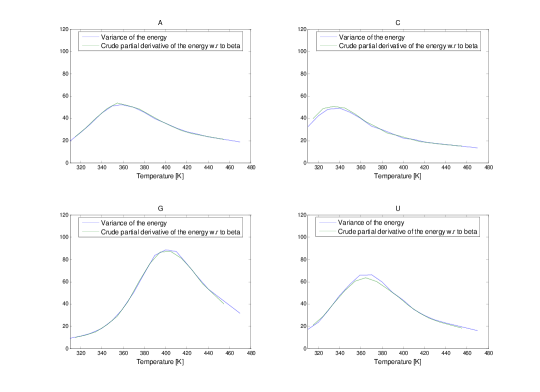

  

  It can be seen that the agreement is good, up to deviations that originate mainly from the relatively large steps in beta and from the higher standard deviations in the internal energy near the peaks.

• The energy distribution function at given betas $\beta_{1},\beta_{2}$ are: $P\left(E,\beta_{1}\right)=\frac{g\left(E\right)exp\left(-\beta_{1}E\right)}{Z_{\beta_{1}}}$, $P\left(E,\beta_{2}\right)=\frac{g\left(E\right)exp\left(-\beta_{2}E\right)}{Z_{\beta_{2}}}$. Hence, we can estimate $P\left(E,\beta_{2}\right)$ using $P\left(E,\beta_{1}\right)$ as follows: $P\left(E,\beta_{2}\right)_{est}=\frac{P\left(E,\beta_{1}\right)exp\left(-E\left(\beta_{2}-\beta_{1}\right)\right)}{\int P\left(E,\beta_{1}\right)exp\left(-E\left(\beta_{2}-\beta_{1}\right)\right)dE}$. The results are shown in the following figure:

  Figure 16: Energy distribution for T=310K,T=320K, and estimation for T=320K with U as the second base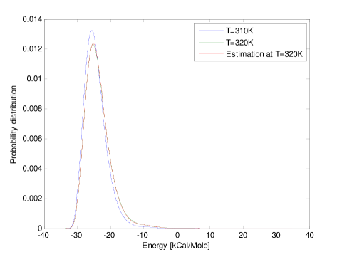

  

  It can be seen that there is good agreement between the energy distribution at T=320K (green line) and the one estimated at T=320K (red line), based on the distribution at T=310K (the red and green lines practically coincide).

• It had to be verified that the integral $\frac{1}{\beta_{1}}\intop_{0}^{\beta_{1}}\left\langle H_{X}\right\rangle d\tilde{\beta}$ is independent of the cutoff energy as discussed in 2.5.5, and the results are shown later on.

2.7.2 Energetically favorable micro-states

We ran the simulation and captured the energetically favorable micro-states in order to asses the energy model. The selected micro-states, and their energy values for the configuration with different bases are presented in the following figures: (1-3 first strand, 4-6 second strand. atoms by their color: white - Hydrogen, blue- Nitrogen, red- Oxygen, green - Carbon)

Figure 17: Micro-state of the system with base A with low energy. Energy values (kCal/Mole): Total -23.12, Stacking -20.46, Hydrogen -5.19, Electrical 1.99, Steric 0.54

Figure 18: Micro-state of the system with base C with low energy. Energy values (kCal/Mole): Total -23.05 , Stacking -20.38, Hydrogen -5.29 , Electrical 1.9 , Steric 0.72

Figure 19: Micro-state of the system with base G with low energy. Energy values (kCal/Mole): Total <23 , Stacking -20.42 , Hydrogen <-8.5, Electrical 2.09, Steric 3.29

Figure 20: Micro-state of the system with base U with low energy. Energy values (kCal/Mole): Total -23.04, Stacking -16.78, Hydrogen -8.63, Electrical 1.88, Steric 0.5

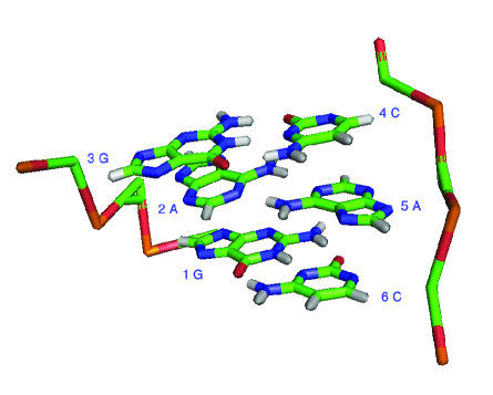
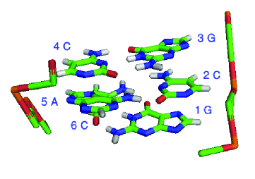
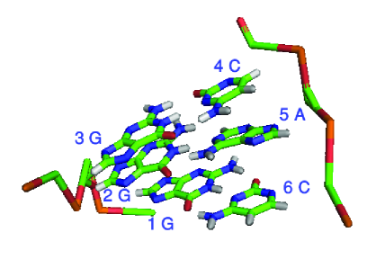
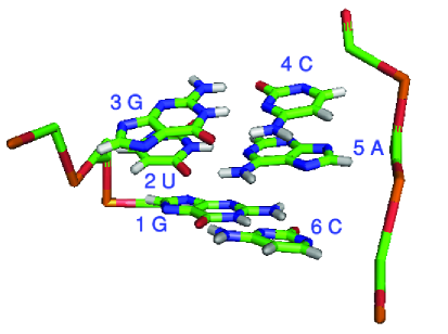
It can be seen that the geometries of the 2nd base with respect to the 5th base in the low energy states are similar to the ones reported in the literature. The A-G pairing geometry is similar to the one presented in [17]. The A-A pairing geometry is also similar to the one presented in [17] and involves Hoogsteen base pairing. The U-A pairing geometry is similar to the well known Watson-Crick Base pairing.

2.7.3 Acceptance rates

The acceptance rates of the internal and external moves as a function of temperature are shown in the following figure:

Figure 21: Acceptance rate of internal and external moves - system with U as the second base

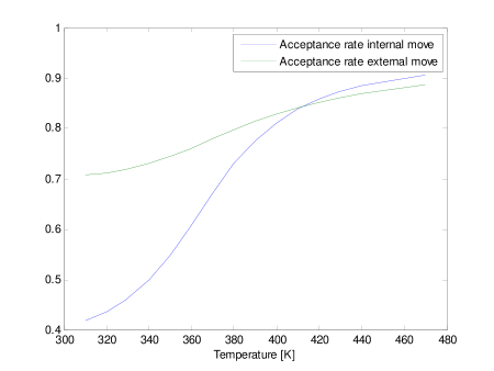
As expected, these acceptance rates are larger for higher temperatures.

The configuration exchange acceptance rates were high since we took small steps in temperature in order to sample well all the temperature range (values around$\sim 0.9$).

2.7.4 Results

Here we present the average of the total, stacking, Hydrogen bond, electrical, and steric energies for the four systems:

Figure 22: The different average energies as a function of temperature for system with the second base A,C

Figure 23: The different average energies as a function of temperature for system with the second base G,U

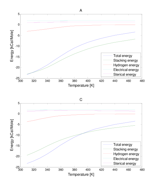
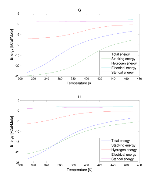
It can be seen that the dominating terms are the stacking and Hydrogen interaction (the Hydrogen interaction energy of the first and last pair aren’t taken into account). As expected all the energies are monotonically increasing function of the temperature. The most significant change is in the stacking and Hydrogen energies since there’s unwinding of the pair in the middle.

The following is a graph of the heat capacity at constant pressure $C_{P}=\left(\frac{\partial H}{\partial T}\right)_{N.P}$ for the four systems:

Figure 24: $C_{p}$ as a function of temperature for the different bases

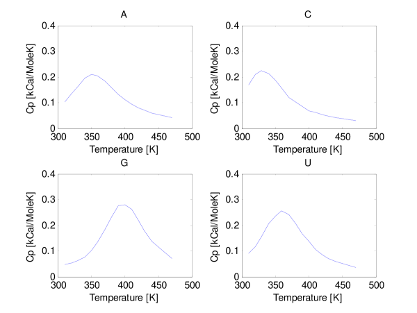
In all the configurations there is a maximum in the heat capacity. This maximum represents the transition from a system in which the dominant energy terms are the stacking and Hydrogen energies to a system which is dominated mainly by the steric energy terms.

Here we present the normalized energy histogram for various temperatures for a system with the second base U:

Figure 25: Normalized energy histogram for different temperatures for a system with the second base U

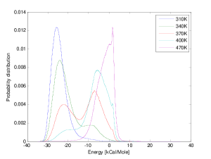
The probability for a given energy for the continuous case is:

$P\left(E\right)=g\left(E\right)e^{-E/kT}/Z$

and in the MC simulation it’s simply the normalized histogram of the energies.

It can be concluded from the graph that there are two peaks in the density of states at these temperatures. This is since there is an increase in the energy distribution that can’t be attributed to $e^{-E/kT}$ . As a result, the standard deviation in the energy at temperatures around 370K is high. The following graphs are the internal energies as a function of $\beta$ :

Figure 26: Internal energy as a function of beta for the different bases

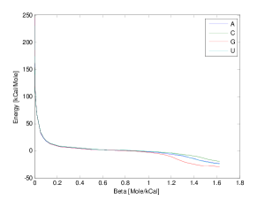
This graph is of high importance since it is being integrated over in the calculation of free energy. The areas differ mainly due to the behavior in the lower temperature regime. The high energy values seen at small $\beta s$ appear because the high temperature enables the molecules to cross one another so the average steric energy is high. In the next figure we compared the energy as a function of $\beta$ for configurations with bases A and C.

Figure 27: Log of the energy as a function of log $\beta$ - comparison between interior loops with A and C

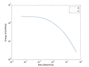
As can be seen from the figure, there is saturation in the energy at small $\beta$s. This is due to the fact that kT at these temperatures is much higher than the energy terms and there is free movement. The fact that the configuration with A has higher internal energy at low $\beta$s can be explained by the higher number of atoms that A contains compared to C, which results in more atoms on average that have high energy terms.

As we raise the cutoff energy, the temperature from which the behavior of the system differs from the original one is higher. Together with it, the internal energy that we’ll have at infinite temperatures will be higher as the molecules are free to enter the volume of one another and will experience higher energies on average (since the cutoff energy is higher). This is in agreement with the assumption that the integral of the internal energies over beta is independent of the cutoff energies as long as we satisfy the relevant conditions. In the following graph we can see that for the higher cutoff we have lower internal energies at $\beta\sim 1\left[Mole/kCal\right]$ and higher internal energies for $\beta<10^{-2}\left[Mole/kCal\right].$ This behavior is more discernible as the difference between the cutoff energies becomes larger.

Figure 28: Log of the energy as a function of log of beta for the two cutoffs - A

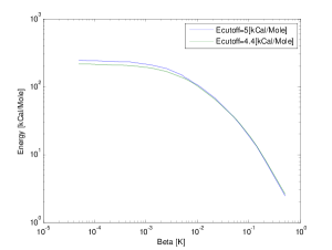
We calculated the values of the integral of the internal energy over $\beta$ for the chosen cutoff energies. The results are shown in the following figure :

Figure 29: Values of the integral for the different cutoff energies (in kCal/Mole) at body temperature

	$E_{\mathrm{cutoff_{1}}}=5kCal/Mole$	$E_{\mathrm{cutoff}_{2}}=4.4kCal/Mole$
$\frac{1}{\beta_{1}}\intop_{0}^{\beta_{1}}\left\langle H_{A}\right\rangle d\tilde{\beta}$	0.73	0.83
$\frac{1}{\beta_{1}}\intop_{0}^{\beta_{1}}\left\langle H_{C}\right\rangle d\tilde{\beta}$	2.22	2.26
$\frac{1}{\beta_{1}}\intop_{0}^{\beta_{1}}\left\langle H_{G}\right\rangle d\tilde{\beta}$	-1.72	-1.66
$\frac{1}{\beta_{1}}\intop_{0}^{\beta_{1}}\left\langle H_{U}\right\rangle d\tilde{\beta}$	1.11	1.01

The integration for the two cutoffs yielded similar results and the differences aren’t far from being in the expected range of error (0.071kCal/Mole, see appendix 3.7.2 for details).

As explained in 2.5.4 the difference between the integrals are the free energy difference between the configurations, meaning that the calculated values are the free energy values of the configurations up to a constant.

Figure 30: Internal energies for the different configurations

	$E_{\mathrm{cutoff_{1}}}=5kCal/Mole$	$E_{\mathrm{cutoff}_{2}}=4.4kCal/Mole$
$U_{A}\left(T=310K\right)$	-23.29	-23.23
$U_{C}\left(T=310K\right)$	-20.04	-19.85
$U_{G}\left(T=310K\right)$	-29.08	-28.97
$U_{U}\left(T=310K\right)$	-24.01	-23.98

Since we have the internal energy of the different configurations (see Fig 30), we can also calculate the entropy difference.

For example, the entropy difference between $A$ and $G$ is calculated as follows for $E_{\mathrm{cutoff_{1}}}=5\left[kCal/Mole\right]$:

$\Delta F_{A\rightarrow G}=\Delta H_{A\rightarrow G}-T\Delta S_{A\rightarrow G}=-5.79-310\cdot\Delta S_{A\rightarrow G}=-2.45\left[kCal/Mole\right]\Rightarrow\Delta S_{A\rightarrow G}=-0.0107\left[kCal/KMole\right],-T\Delta S_{A\rightarrow G}=3.34\left[kCal/Mole\right]$

For $E_{\mathrm{cutoff}_{2}}=4.4\left[kCal/Mole\right]$ we have:

$\Delta F_{A\rightarrow G}=\Delta H_{A\rightarrow G}-T\Delta S_{A\rightarrow G}=-5.74-310\cdot\Delta S_{A\rightarrow G}=-2.49\left[kCal/Mole\right]\Rightarrow\Delta S_{A\rightarrow G}=-0.0105\left[kCal/KMole\right],-T\Delta S_{A\rightarrow G}=3.25\left[kCal/Mole\right]$

It can be seen that there is $\sim 2\%$ deviation in the entropy value between the systems with the two cutoffs. This deviation can be minimized by using higher cutoffs (the cutoffs satisfy $E_{\mathrm{cutoff_{1}}}\approx 7kT_{body},E_{\mathrm{cutoff_{2}}}\approx 8kT_{body}$) and larger number of iterations in the MC simulations.

We can also calculate the entropies for higher temperatures in the same manner. Results are shown in the following figure:

Figure 31: $\Delta S_{A\rightarrow G}$ as a function of temperature

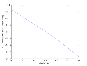
The entropy difference in absolute value gets larger as we raise the temperature. The entropy is a monotonically increasing function of the internal energy, which is a monotonically increasing function of the temperature. Hence, as we increase the temperature, the entropies are expected to get larger and it’s likely that the entropy difference between the systems will also be such.

2.8 Discussion

In conclusion, we presented models for faces and the interactions in RNAs and introduced a procedure to calculate the free energy of interior loops, and faces in general. This procedure, if verified or improved may suggest an alternative to the experiments in which free energy of faces are calculated. Under the assumptions that the secondary structure is known and that faces are decoupled, simulations on several faces can also be performed together to generate the whole tertiary structure, and more global properties can be collected. In the calculation of free energy we showed a method in which the information gathered in the course of parallel tempering can be used to calculate the free energy difference between systems. In this method, if the energy landscape is rugged, instead of sampling both over the space of $\lambda$, the parameter related to the TI procedure, and the temperature, we sample just over the temperatures of the configurations of interest (up to infinity). This method is much easier to implement than ThI and is likely to be much faster in rugged energy landscapes. This is crucial when the cost of the calculation is high, as is often the case in RNA tertiary structures simulations. In the method we had to bring the two systems to regimes at which the partition functions are equal. Although this is easily satisfied for systems that have the same $\beta\rightarrow 0$ limit, we wanted the condition to be satisfied for all systems that have the same degrees of freedom. We introduced a cutoff energy in the repulsion term which enabled the molecules to enter the “volume” of one another and as a result the condition could be satisfied. This use cutoff energy can also be applied to other methods such as ThI and enable the calculation of free energy in the cases where the sampling of the integrand isn’t feasible.

Regarding the optimization of software written in c/c++ languages, though the range of possible actions is huge, if the bottlenecks are identified and the relevant actions are performed (as listed in 2.6.2), together with the use of the proper compiler, and the capabilities of vectorization of the processor, a tremendous improvement in the running time can be achieved in a relatively short time.

2.8.1 Improvement proposals

As reported by [30], the backbone bond angles defined in our model are in the range of $90^{\circ}-120^{\circ}$. The P-C-N bond angle also showed small standard deviation by PDB analysis. In order to take it into account we can add the following energy terms:

$H_{\mathrm{bond\,angle}}=\underset{i}{\sum}\frac{1}{2kT}\left[\left(\frac{\theta_{PCP_{i}}-\theta_{PCP_{avg}}}{\sigma_{\theta_{PCP}}}\right)^{2}+\left(\frac{\theta_{CPC_{i}}-\theta_{CPC_{avg}}}{\sigma_{\theta_{CPC}}}\right)^{2}+\left(\frac{\theta_{PCN_{i}}-\theta_{PCN{}_{avg}}}{\sigma_{\theta_{PCN}}}\right)^{2}\right]$

Alternatively, we can switch to full atomistic modelling of the backbone and the ribose. As will become clear later, this modelling will include 7 degrees of freedom per nucleotide for the seven torsion angles. A CONROT (concerted rotation) Monte-Carlo move can be used, in which 7 consecutive torsion angles are changed keeping the bond angles, distances and the rest of the configuration fixed [31, 32]. As the backbone torsion angle $\delta$ is directly correlated to the ribose dihedral angle $\nu_{3}$ which determines the ribose configuration [33], it seems that the ribose doesn’t introduce a degree of freedom [15] other than the torsion angle $\chi$ that defines the orientation of the base with respect to the ribose. Since the faces are assumed to be decoupled from one another, the configuration of the ribose and hence $\delta$ and the torsion angle $\chi$ have to be constant in the nucleotides that are shared by two faces. Hence, the degrees of freedom that we have consist of the 7 torsion angles $\alpha,\beta,\gamma,\delta,\varepsilon,\zeta,\chi$ for the nucleotides that are not shared between faces and 5 torsion angles $\alpha,\beta,\gamma,\varepsilon,\zeta$ for the nucleotides that are shared between faces. A more natural choice of division of the atoms that belong to a nucleotide would be C4’ to C4’ since the faces are assumed to be decoupled

The ribose also has $\delta$ dependent energy landscape [33] which can be taken into account.

Regarding the Monte Carlo moves, we can perform the following moves:

• CONROT move in the backbone that won’t change $\delta$ of the unshared nucleotides.

• Rotation of the $\chi$ torsion angle in the unshared nucleotides.

• A move that will affect the location of the ribose and the base of the shared nucleotides and that will keep $\delta_{1},\chi_{1},\delta_{2},\chi_{2}$ constant. Such a move can be the following: we can define virtual bond $C3^{\prime}_{1}-C4^{\prime}_{2}$ that connects the two shared nucleotides. Since the bond and torsion angles between these atoms are assumed to be constant, the length of this bond can be considered to be fixed. Since rotation around the $\varepsilon$ or $\gamma$ torsion angle rotates the virtual bond, the virtual bond angles $O3^{\prime}_{1}-C3^{\prime}_{1}-C4^{\prime}_{2},\,C3^{\prime}_{1}-C4^{\prime}_{2}-C5^{\prime}_{2}$ can be considered fixed. Now, since the requirements for the CONROT move are satisfied (fixed bond length and bond angle), the $C3^{\prime}_{1}-C4^{\prime}_{2}$ can be considered as a bond in a CONROT move that includes two more atoms and involves the changing the location of the ribose and the base of the shared nucleotides. This use of virtual bonds in the CONROT move is rather general and can be used in other places.

3 Appendixes

3.1 Description of the algorithm for re-generating structures

The software reads the string of ’(’, ’.’ and ’)’ characters from left to right and processes the information iteratively. In each iteration, the software runs over the ’(’ and ’.’ characters until it reaches a ’)’ character. In this process it saves the indexes of the ’(’ characters in the “bases to be paired” list. Then it runs over the ’)’ characters and pairs them with the bases from the list (saves them in the “paired bases” list) until it reaches a ’(’ character. At this point we have a list of “paired bases” and a list of “bases to be paired” . Here we stop to define a process in which a son is generated and all the paired bases are moved to it (which will be called “process” from now on). We also mention here that each structure has, as one of its fields, the number of unpaired bases after the process (The initial value for this field is -1). If, at this point of the iteration, there are more unpaired bases in the list, a process is done - a son is generated, and the pairs are stored in it (we’ll call this condition 1). If, it continued the pairing task with the father (if during the iteration, there are more ’)’ characters after all the bases have been paired, it will continue the pairing task with the father $\left(*\right)$) , and the father’s substructure has less unpaired bases, than it had before, it means that it detected a multiloop (called condition 2). In that case, a son which is a multiloop is created and all the structure’s sons are moved to it. If a son was generated, in the next iteration, if a ’(’ is detected first, then a new son is generated, and the iteration is processed with this son $\left(**\right)$.

For example, for the following string:

$\begin{array}[]{c}(....(....)....(...(...)....(....)...)....(....)....)\\ A..B...B^{\prime}...C..D.D^{\prime}..E..E^{\prime}..C^{\prime}..F..F^{\prime}..A^{\prime}\end{array}$

(Where the letters specify locations in the string).

Using the algorithm specified above we’ll have the following steps:

iteration	1	2	3	4
starting point	$A$	$C$	$E$	$F$
ending point	$C$	$E$	$F$	$A^{\prime}$
conditions fulfilled during the iteration			$\left(*\right)$,$\left(**\right)$	$\left(*\right)$,$\left(**\right)$
list of pairs after the iteration	$BB^{\prime}$	$DD^{\prime}$	$EE^{\prime}$
list of bases to be paired after the iteration	$A$	$A,C$	$A$
condition fulfilled after the iteration	1	1	2	2

Where * is used the specify the structure that the algorithm begins the iteration with.

The software can give as an output pairs, faces and nucleotide’s sequences for each substructure.

3.2 Description of the algorithm for comparing structures

For the first structure, it runs over all faces, and for each face, it looks for identical ones in the second structure. If it finds an identical face, it updates the faces’ field similarity level to identical. It then removes it from the list of faces of the first and second structure and adds it to lists of similar faces, in order (identical face is also similar).

Then it runs over the nonidentical faces in the first structure and for each face, it looks for similar faces in the second structure. In case it finds a similar face, it updates the faces’ field similarity level to similar. It then removes them from the list of faces of the first and second structure and adds it to the new lists. Then it generates one vector for the first structure and one vector for the second structure that include the different faces. It then sorts them according to the face type (hairpin loop, stacking region bulge, interior loop or multiloop). Thus it enables us to see which faces are preferred over which faces in the two structures.

3.3 Experimental calculation of free energy

3.3.1 General method

Say we have two strands of RNA that can bind in the following reaction:

$$\left[A\right]+\left[B\right]\rightarrow\left[AB\right]$$ (30)

where $\left[A\right],\left[B\right]$ denote the concentrations of the single strands and $\left[AB\right]$ denotes the concentration of their bound product.

The free energy difference is:

$$\triangle G=-RTlnK$$ (31)

Where the dissociation constant $K$ is defined as follows:

$$K\triangleq\frac{\left[AB\right]}{\left[A\right]\left[B\right]}$$ (32)

At $T_{m}$, by definition, the concentration of the reactors and the products is equal.

Say we take an initial concentration of the reactors of $\left[A\right]=\left[B\right]=\frac{X_{0}}{2}$, and zero initial concentration of the product $\left[AB\right]=0$.

According to the reaction, it can be seen that at $T_{m}$ (where $T_{m}$ denotes melting temperature) we have:

$\left[A\right]=\left[B\right]=\left[AB\right]=\frac{X_{0}}{4}$.

Substituting it in (31), we get:

$$\triangle G_{T_{m}}=-RTlnK_{T_{m}}=RTln\left(\frac{X_{0}}{4}\right)$$ (33)

We can use:

$$\triangle G_{T_{m}}=\triangle H\left(T_{m}\right)-T_{m}\triangle S\left(T_{m}\right)$$ (34)

and get:

$$\frac{1}{T_{m}}=\frac{R}{H\left(T_{m}\right)}ln\left(\frac{X_{0}}{4}\right)+\frac{\triangle S\left(T_{m}\right)}{\triangle H\left(T_{m}\right)}$$ (35)

Now each time the initial concentration of the reactors is changed and $T_{m}$ is measured.

Thus, a graph of $\frac{1}{T_{m}}$ as a function of $ln\left(\frac{X_{0}}{4}\right)$ can be generated.

From this graph $\triangle H\left(T_{m}\right),\triangle S\left(T_{m}\right)$ can be extracted.

It is here to mention that the product consists of many faces and the values of the enthalpy and entropy are assigned by fitting results to the faces from many experiments.

3.3.2 Finding enthalpy and entropy values at body temperature

Even if we assume that the former experiments are performed in a small range of temperatures, in which the enthalpy and entropy are constant, it can’t be assumed that these temperatures are close to body temperature.

Measuring the heat capacity as a function of temperature enables the calculation of the enthalpy and entropy values at body temperature.

$$C_{p}=\left(\frac{dQ}{dT}\right)_{P}$$ (36)

The enthalpy and entropy can be expressed as functionals dependent on the function of heat capacity over temperature.

Since the process is quasistatic:

$dQ=TdS$ , and we can write:

$$\left(\frac{dS}{dT}\right)_{P}=\frac{1}{T}C_{P}$$ (37)

Regarding the enthalpy:

$H\left(S,P,N\right)$ since it’s a function of $S,P$ and $N$ and $P,N$ are held constant we can write the derivative of the enthalpy with respect to the temperature as follows:

$$\left(\frac{\partial H}{\partial T}\right)_{P,N}=\frac{\partial H}{\partial S}\frac{\partial S}{\partial T}=T\frac{1}{T}C_{P}=C_{p}$$ (38)

So we can write:

$$\triangle H\left(T_{body}\right)=\triangle H\left(T_{m}\right)+\int_{T_{body}}^{T_{m}}C_{p}dT$$ (39)

$$\triangle S\left(T_{body}\right)=\triangle S\left(T_{m}\right)+\int_{T_{body}}^{T_{m}}\frac{1}{T}C_{p}dT$$ (40)

And In conclusion :

$\triangle H\left(T_{m}\right),\triangle S\left(T_{m}\right),C_{p}\left(T\right)\Rightarrow\triangle H\left(T_{body}\right),\triangle S\left(T_{body}\right)$

However, in many calculations, dependency of the heat capacity on the temperature was neglected, so the experiments are to be redone.

3.4 Agreement between the Metropolis criteria to detailed balance

According to the detailed balance criteria, it can be written for the canonical ensemble:

$$\frac{P\left(i\rightarrow j\right)}{P\left(j\rightarrow i\right)}=\frac{P\left(j\right)}{P\left(i\right)}=\frac{e^{-\beta H_{j}}}{e^{-\beta H_{i}}}=e^{-\beta\left(H_{j}-H_{i}\right)}=$$ (41)

$$\frac{min\left\{1,e^{-\beta\left(H_{j}-H_{i}\right)}\right\}}{min\left\{1,e^{+\beta\left(H_{j}-H_{i}\right)}\right\}}$$ (42)

So for the choice of

$$P\left(i\rightarrow j\right)=min\left\{1,e^{-\beta\left(H_{j}-H_{i}\right)}\right\},P\left(j\rightarrow i\right)=min\left\{1,e^{+\beta\left(H_{j}-H_{i}\right)}\right\}$$ (43)

detailed balance is fulfilled.

3.5 Thermodynamic integration

Thermodynamic integration is a method to calculate free energy differences between two systems (in our case they can differ by of a base).

In the method a parameter that transforms the first system to the second one is introduced.

We can define $A$ as the first system, and $B$ as the second system.

We can write the free energy difference as follows:

$$\triangle F_{A\rightarrow B}\left(\beta_{1}\right)=\intop_{0}^{1}\frac{dF_{\lambda}}{d\lambda}d\lambda=$$ (44)

Where $\lambda$ is a general parameter. We can substitute $F=-kTlnZ$ and get:

$$-kT\intop_{0}^{1}\frac{dlnZ}{d\lambda}d\lambda=$$

$$-kT\intop_{0}^{1}\frac{1}{Z}\frac{dZ}{d\lambda}d\lambda=$$

Substituting $Z=\int e^{-\beta H}d\Omega$ we get:

$$-kT\intop_{0}^{1}\frac{1}{Z}\frac{\int e^{-\beta_{1}H}d\Omega}{d\lambda}d\lambda=$$

$$kT\intop_{0}^{1}\frac{1}{Z}\int e^{-\beta_{1}H}\frac{dH}{d\lambda}d\Omega\beta_{1}d\lambda=$$

$$\intop_{0}^{1}\frac{\int e^{-\beta_{1}H}\frac{dH}{d\lambda}d\Omega}{Z}d\lambda=$$

$$\intop_{0}^{1}\left\langle\frac{dH}{d\lambda}\right\rangle d\lambda=$$

For a choice of:

$$H=\lambda H_{B}+\left(1-\lambda\right)H_{A}$$ (45)

We have for

$$\frac{dH}{d\lambda}=H_{B}-H_{A}$$

And it can be written:

$$\triangle F_{A\rightarrow B}\left(\beta_{1}\right)=\intop_{0}^{1}\left\langle H_{B}-H_{A}\right\rangle d\lambda$$ (46)

Or in a more explicit form:

$$\triangle F_{A\rightarrow B}\left(\beta_{1}\right)=\intop_{0}^{1}\frac{\left\{\int\left(H_{B}-H_{A}\right)e^{-\beta_{1}\left[\lambda H_{B}+\left(1-\lambda\right)H_{A}\right]}d\Omega\right\}}{\int e^{-\beta_{1}\left[\lambda H_{A}+\left(1-\lambda\right)H_{B}\right]}d\Omega}d\lambda$$

3.6 Parameters chosen for the simulation

3.6.1 Temperatures chosen for the free energy calculation

In order to perform the integration, the following temperatures were chosen:

• range 1: 310 320 329 340 350 359 370 380 390 400 410 420 429 440 470

• range 2: 500 580 670 780 890 1000

• range 3: 1000 2285 3571 4857 6142 7428 8714

• range 4: 10000 22857 35714 48571 61428 74285 87142

• range 5: 100000 200000 400000 1000000 10000000

3.7 Standard deviations in the measurements

3.7.1 Standard deviation in the calculation of the internal energy

We can estimate the number of steps it takes for two configurations to be independent, by the average number of steps it takes for a replica of the system in a given temperature to exchange configuration with a replica of the system in an adjacent temperature, multiplied by the square of the number of temperatures. Since the average number of steps for a configuration exchange is the number of steps after which we attempt to exchange, divided the acceptance rate, we can estimate the number of independent measurements in the following way: $n=\frac{\mathrm{MC\,moves}}{\mathrm{\left(steps\mathrm{\,for\,a\,configuration\,exchange\,attempt/acceptance\,rate}\right)\cdot N^{2}}}$

For a temperature in the first temperature range we can write:

$n=\frac{2\cdot 10^{8}\cdot 0.9}{910\cdot 225}=879$ (where $n$ is the number of independent measurements).

Since the standard deviation of the average of n independent variables with a standard deviation $\sigma_{i}$ is:

$\sigma_{A}=\frac{\sigma_{i}}{\sqrt{n}}$, we can use it to estimate the standard deviation of the internal energy.

For example for the first temperature, we can substitute the standard deviation of the energy from the simulation and get:

$\sigma_{T}=\frac{\sigma_{L}}{\sqrt{n}}=\frac{4.148}{29.64}=0.14\left[kCal/Mole\right]$

3.7.2 Standard deviation in the calculation of the free energy

In the free energy calculation, we integrate numerically the average energy over function of beta:

$\frac{1}{\beta_{1}}\left[\intop_{0}^{\beta_{1}}\left\langle H_{X}\right\rangle d\tilde{\beta}\right]$

It is done by estimating the area between two points as the average energy multiplied by the difference in $\beta$.

$F_{X}=\frac{1}{\beta_{1}}\left[\intop_{0}^{\beta_{1}}\left\langle H_{X}\right\rangle d\tilde{\beta}\right]=\frac{1}{\beta_{1}}\underset{i}{\sum}\left(\left\langle H_{X}\left(\beta_{i}\right)\right\rangle+\left\langle H_{X}\left(\beta_{i+1}\right)\right\rangle\right)/2\cdot\Delta\beta_{i}$

The standard deviation and the error range can be calculated as follows:

$\sigma_{F_{x}}=\frac{1}{2\beta_{1}}\sqrt{\left(\underset{i}{\sum}\sigma_{\left\langle H_{X}\left(\beta_{i}\right)\right\rangle}^{2}+\sigma_{\left\langle H_{X}\left(\beta_{i+1}\right)\right\rangle}^{2}\right)\cdot\Delta\beta_{i}^{2}}=0.0355kCal/Mole$

$\Rightarrow\mathrm{error}\mathrm{\,range\sim 2}\sigma_{F_{x}}=0.071kCal/Mole$

References

- [1] M. Zuker and P. Stiegler. Optimal computer folding of large RNA sequences using thermodynamics and auxiliary information. Nucleic acids research, 9(1):133, 1981.
- [2] K. Fejes-Toth, V. Sotirova, R. Sachidanandam, G. Assaf, G.J. Hannon, P. Kapranov, S. Foissac, A.T. Willingham, R. Duttagupta, E. Dumais, et al. Post-transcriptional processing generates a diversity of 5?-modified long and short RNAs. Nature, 457(7232):1028–1032, 2009.
- [3] G.V. Kryukov, S. Castellano, S.V. Novoselov, A.V. Lobanov, O. Zehtab, R. Guigo, and V.N. Gladyshev. Characterization of mammalian selenoproteomes. Science, 300(5624):1439, 2003.
- [4] D. Fagegaltier, A. Lescure, R. Walczak, P. Carbon, and A. Krol. Structural analysis of new local features in SECIS RNA hairpins. Nucleic Acids Research, 28(14):2679, 2000.
- [5] Y. Ito, Y. Sone, and T. Mizutani. Stability of non-Watson-Crick GA/AG base pair in synthetic DNA and RNA oligonucleotides. Molecular Biology Reports, 31(1):31–36, 2004.
- [6] Y. Ito and T. Mizutani. Evidence of GA/AG pair, not AG/GA pair, in SECIS element. In Nucleic Acids Symposium Series, volume 1, page 41. Oxford Univ Press, 2001.
- [7] S.E. Morse and D.E. Draper. Purine–purine mismatches in RNA helices: evidence for protonated G· A pairs and next-nearest neighbor effects. Nucleic acids research, 23(2):302, 1995.
- [8] Clark C. Barciszewski J, Frederic B. RNA biochemistry and biotechnology., pages 73–87, 1999.
-
[9]
C. Schneider, M. Brandl, M. Meyer, and J. S
"uhnel. Water-Mediated Uracil-Cytosine Base Pairs in RNA-A Computational Study. - [10] J.G. Kirkwood. Statistical mechanics of fluid mixtures. The Journal of Chemical Physics, 3:300, 1935.
- [11] TP Straatsma and JA McCammon. Multiconfiguration thermodynamic integration. The Journal of chemical physics, 95:1175, 1991.
- [12] D. Frenkel and B. Smit. Understanding molecular simulation: from algorithms to applications. Academic Press, Inc. Orlando, FL, USA, 1996.
- [13] W.K. Olson. Configurational statistics of polynucleotide chains. A single virtual bond treatment. Macromolecules, 8(3):272–275, 1975.
- [14] K.S. Keating and A.M. Pyle. Semiautomated model building for RNA crystallography using a directed rotameric approach. Proceedings of the National Academy of Sciences, 107(18):8177, 2010.
- [15] L.J.W. Murray, W.B. Arendall, D.C. Richardson, and J.S. Richardson. RNA backbone is rotameric. Proceedings of the National Academy of Sciences of the United States of America, 100(24):13905, 2003.
- [16] Wolfarm Saenger. Principles of Nucleic Acid Structure. page 125, 1984.
- [17] N.B. LEONTIS and E. Westhof. Geometric nomenclature and classification of RNA base pairs. Rna, 7(04):499–512, 2001.
- [18] C. Smith P.J Struther Arnott and R. Chandrasekaran. Handbook of biochemistry and Molecular Biology. pages 411–422, 1976.
- [19] A. Rich, D.R. Davies, FHC Crick, and JD Watson. The molecular structure of polyadenylic acid. Journal of molecular biology, 3(1):71–86, 1961.
- [20] Wolfarm Saenger. Principles of Nucleic Acid Structure. page 40, 1984.
- [21] Arthur J. Olson. Van der waals potential energy.
- [22] Wolfarm Saenger. Principles of Nucleic Acid Structure. page 139, 1984.
- [23] A. Vedani. YETI: An interactive molecular mechanics program for small-molecule protein complexes. Journal of Computational Chemistry, 9(3):269–280, 1988.
- [24] T.A. Knotts IV, N. Rathore, D.C. Schwartz, and J.J. De Pablo. A coarse grain model for DNA. The Journal of chemical physics, 126:084901, 2007.
- [25] J. Parsons, J.B. Holmes, J.M. Rojas, J. Tsai, and C.E.M. Strauss. Practical conversion from torsion space to Cartesian space for in silico protein synthesis. Journal of computational chemistry, 26(10):1063–1068, 2005.
- [26] U.H.E. Hansmann. Parallel tempering algorithm for conformational studies of biological molecules. Chemical Physics Letters, 281(1-3):140–150, 1997.
- [27] D.J. Earl and M.W. Deem. Parallel tempering: Theory, applications, and new perspectives. Physical Chemistry Chemical Physics, 7(23):3910–3916, 2005.
- [28] William Kahan. Further remarks on reducing truncation errors. Communications of the ACM, 8(1):40,48, 1965.
- [29] Pete Isensee. C++ optimization strategies and techniques.
- [30] R. Malathi and N. Yathindra. Virtual bond probe to study ordered and random coil conformations of nucleic acids. International Journal of Quantum Chemistry, 20(1):241–257, 1981.
- [31] LR Dodd, TD Boone, and DN Theodorou. A concerted rotation algorithm for atomistic Monte Carlo simulation of polymer melts and glasses. Molecular Physics, 78(4):961–996, 1993.
- [32] J.P. Ulmschneider and W.L. Jorgensen. Monte Carlo backbone sampling for nucleic acids using concerted rotations including variable bond angles. The Journal of Physical Chemistry B, 108(43):16883–16892, 2004.
- [33] Wolfarm Saenger. Principles of Nucleic Acid Structure. page 60, 1984.