Numerical Study of the Overlap Lee-Yang Singularities in the Three-Dimensional Edwards-Anderson Model

Abstract

We have characterized numerically, using the Janus computer, the Lee-Yang complex singularities related to the overlap in the $3D$ Ising spin glass with binary couplings in a wide range of temperatures (both in the critical and in the spin-glass phase). Studying the behavior of the zeros at the critical point, we have obtained an accurate measurement of the anomalous dimension in very good agreement with the values quoted in the literature. In addition, by studying the density of the zeros we have been able to characterize the phase transition and to investigate the Edwards-Anderson order parameter in the spin-glass phase, finding agreement with the values obtained using more conventional techniques.

1 Introduction

In two seminal papers, T. D. Lee and C. N. Yang [1, 2] introduced a new tool to understand the origin of a phase transition by studying the complex singularities of the free energy, or, equivalently, the zeros of the partition function. In particular, they showed that all the zeros are located on the unit circumference on the complex activity plane (taking as variable $z=e^{-2h}$, where $h$ is the external magnetic field). They also proved that if the zeros condense onto the real axis when $V\rightarrow\infty$ a phase transition takes place. Finally, they related, in the low-temperature phase, the density of zeros with the discontinuity in the order parameter (remember that the Ising model experiences a first-order phase transition when $h$ changes at a fixed temperature below the critical one). This approach was subsequently extended to the temperature zeros by Fisher [3, 4, 5, 6].

We have Lee-Yang like theorems only for a limited class of non-disordered systems (such as Ising models). However, it is possible to develop a scaling theory by assuming that asymptotically the complex singularities (wherever they lie) touch the real axis (thus generating the phase transition). Hence, despite the lack of formal theorems it is still possible to apply Lee and Yang’s main results to a wide class of systems (e.g., Potts models [7]). In this class of systems the zeros do not live on a circle as stated by the Lee-Yang theorem, but they still control the critical properties of the model. We will only assume this last fact irrespectively of the form of the locus of the zeros in the complex plane [7].

In Refs. [8, 9, 10] the analysis of complex singularities was applied successfully to diluted systems (in particular diluted Ising models in two and four dimensions). The key point for the applicability of the standard results, well tested in non-disordered systems, is to compute the complex singularities individually for each disorder realization (called sample) and then use the mean of the individual zeros (sample zeros) in order to test the scaling properties of the zeros and to study the properties of the integrated density of zeros. In this work we will also introduce the analysis of the median.

Nowadays we are interested in gaining a deeper understanding (from the point of view of the complex singularities) of the properties of an interesting frustrated and disordered system: the three-dimensional Ising spin glass. The magnetization, while very interesting in off-equilibrium dynamics and in experiments, plays no role in the critical behavior and in the understanding of the low-temperature properties in a finite-dimensional spin glass. The observable that controls this spin-glass phase is the overlap. Hence, in this work we have focused on the numerical study of the complex singularities linked with the overlap in order to study the phase transition and the properties of the spin-glass phase.

In the past, Lee-Yang and Fisher zeros were obtained in spin glasses by means of the numerical evaluation of the partition function on small lattices [11, 12, 13, 14]. This methodology was also applied to models defined on Bethe lattices [15]. Finally, some calculations were performed with the help of replicas [16].

More recently, the complex singularities linked with the external magnetic field were studied for the two and three-dimensional Ising spin glass model in the interesting reference [17], which focuses on the Griffiths singularity and computes all the zeros for small lattices.

In particular we are interested in characterizing the scaling of the individual zeros at the critical point (which will allow us to compute the anomalous dimension exponent) and checking the scaling in the spin-glass region. In addition, we want to study the properties of the density of zeros in the critical and spin-glass region: the behavior of this observable will clearly signal the phase transition. Finally, we will show how this density of zeros can be used to compute the Edwards-Anderson order parameter. However, the spin-glass susceptibility presents strong scaling corrections (even on an $L=32$ lattice and $\beta=1.4$), which induce strong corrections on the density of zeros allowing us (from the numerical point of view) only to test our density of zeros against the values of $q_{\mathrm{EA}}$ found in the literature, rather than attempting a direct numerical computation of the order parameter. We want to stress that in cases in which the spin glass susceptibility reaches the asymptotic value, the method we propose will be able to provide directly the order parameter ($q_{\mathrm{EA}}$) giving an additional method to those used nowadays [18, 19, 20, 21].

Let us finally mention that we have obtained the data presented in this work from the analysis of the configurations produced in parallel tempering runs [20, 21] using the Janus computer [22, 23, 24].

2 Model and observables

We have studied the three-dimensional Edwards-Anderson model with dynamical variables $\sigma_{i}$. These variables are Ising spins and are placed on the nodes of a cubic lattice of linear dimension $L$ and volume $V=L^{3}$. The Hamiltonian of the system is

$$\mathcal{H}_{0}=-\sum_{\langle i,j\rangle}J_{ij}\sigma_{i}\sigma_{j},$$ (1)

where $\langle ij\rangle$ indicates that the sum is over the nearest neighbouring sites. The couplings $J_{ij}$ are random quenched constants with bimodal probability distribution, that is, $J=\pm 1$ with $50\%$ probability. Every realization of the couplings is called a sample. Due to the fact that we have a random Hamiltonian, we have to deal with a double average: first the thermal average, which we will denote by $\langle(\cdots)\rangle$, and then the average over the samples, which we will denote by $\overline{(\cdots)}$.

We have simulated several real replicas of the system, so we can define the local overlap

$$q_{i}=\sigma_{i}^{(1)}\sigma_{i}^{(2)}$$ (2)

where $\sigma_{x}^{(1)}$ belongs to the first replica and $\sigma_{x}^{(2)}$ belongs to the second one. The spin overlap is defined from this local overlap as

$$Q=\sum_{i}q_{i},$$ (3)

where the sum runs over the whole volume ($V$). In addition, we define $q\equiv Q/V$. These observables allow us to define some new quantities, for example the non-connected spin-glass susceptibility

$$\chi_{\mathrm{SG}}=\frac{1}{V}\overline{\langle Q^{2}\rangle}.$$ (4)

Let us now rewrite the Hamiltonian adding a new perturbation $\epsilon Q$ and including the two replicas explicitly,

$$\displaystyle\mathcal{H}_{\epsilon} = \mathcal{H}(\sigma_{1})+\mathcal{H}(\sigma_{2})+\epsilon Q$$ (5)

$$= -\sum_{\langle i,j\rangle}J_{ij}\left(\sigma_{i}^{(1)}\sigma_{j}^{(1)}+\sigma_{i}^{(2)}\sigma_{j}^{(2)}\right)+\epsilon\sum_{i}\sigma_{i}^{(1)}\sigma_{i}^{(2)}.$$

This Hamiltonian looks like that of the Ising model in a magnetic field

$$\mathcal{H}_{h}=\mathcal{H}_{0}+h\mathcal{M}.$$ (6)

We can write the partition function, whose zeros we want to study, as

$$\displaystyle Z = \sum_{[\sigma^{(1)}\sigma^{(2)}]}e^{-\beta\mathcal{H}_{0}+\beta i\epsilon Q}$$

$$= \sum_{[\sigma^{(1)}\sigma^{(2)}]}\left(\cos(\beta\epsilon Q)e^{-\beta\mathcal{H}_{0}}+i\sin(\beta\epsilon Q)e^{-\beta\mathcal{H}_{0}}\right).$$

Let $Z_{0}$ the partition function of the non-perturbed system, so

$$Z=Z_{0}\{\langle\cos(\beta\epsilon Q)\rangle+i\langle\sin(\beta\epsilon Q)\}$$ (8)

and we have to find the zeros of the function $\langle\cos(\beta\epsilon Q)\rangle$ since in absence of a magnetic field $\langle\sin(\beta\epsilon Q)\rangle$ is zero. The algorithm to find them is quite easy: we start from the list of individual measurements of $Q$ for each sample (see Section 4) and evaluate the average $\langle\cos(\beta\epsilon Q)\rangle$, increasing $\epsilon$ in small steps $\Delta\epsilon$. When the function changes signs from one step to the next, we have found a zero in this interval. Obviously, the smaller $\Delta\epsilon$ the better the precision of the zero that we have found, but also the slower the analysis, so we have to be careful with the error estimates. We have analyzed the first four zeros of this function.

3 Finite-Size Scaling

One can obtain the expected behavior of the LY zeros by means of (see for example Ref.  [7])

$$\epsilon\simeq\frac{1}{\sqrt{\chi_{\mathrm{SG}}V}}\,$$ (9)

therefore, the finite-size dependence, at the critical point, of the Yang-Lee zeros can be expressed as:

$$\epsilon_{j}(L)\sim L^{-x_{1}}\,,$$ (10)

where

$$x_{1}=(D+2-\eta)/2\,,$$ (11)

and $D$ is the dimensionality of the system, being $D=3$ in this work. If corrections to scaling are taken into account, the above relation becomes

$$\epsilon_{j}(L)\sim L^{-x_{1}}\left(1+{\cal O}(L^{-x_{2}})\right)\,,$$ (12)

where $x_{2}$ is the leading correction-to-scaling exponent, $x_{2}=\omega$.

In the broken symmetry phase, where the non-linear susceptibility diverges as the volume of the system, we expect the following behavior:

$$\epsilon_{j}(L)\sim\frac{1}{V}\,,$$ (13)

We can take scaling corrections into account, as in the critical point, and

$$\epsilon_{j}(L)\sim V^{-1}\left(1+{\cal O}(L^{-x_{3}})\right)\,.$$ (14)

where $x_{3}$ is the leading correction-to-scaling exponent in the broken phase..

In order to discuss the density of zeros we need to describe some known properties of the Hamiltonian defined in Eq. (5). This Hamiltonian was introduced in the past [25, 26]. In particular it experiences a first-order phase transition in $\epsilon$, below the critical temperature of the uncoupled model. Hence, the overlap is discontinuous:

$$\lim_{\epsilon\to 0^{\pm}}\overline{\langle q\rangle}(\epsilon)=\pm q_{\mathrm{EA}}\,,$$ (15)

being the discontinuity at the transition just $2q_{\mathrm{EA}}$.

We can also introduce the density of zeros

$$\mu_{\epsilon}(\epsilon)=\sum_{j}\delta(\epsilon-\epsilon_{j}(L))$$ (16)

and its integrated version

$$G(\epsilon)=\int_{0}^{\epsilon}dx\mu_{\epsilon}(x)$$ (17)

which takes the following value computed for a given zero:

$$G(\epsilon_{j}(L))=\frac{2j-1}{2V}\,,$$ (18)

where $j$ labels the $j$-th zero ($j=1,2,\ldots$). In order to deal with the discontinuous behavior of $G(\epsilon)$ at the zeros, we follow the recipe of references [27, 28] and use the mean between two consecutive plateau values ($j-1$ and $j$). Anyhow, the asymptotic value of the integrated density computed in the $j$-th zero is $j/V$. We will discuss this point again in subsection 5.3.

This integrated density is very useful to characterize a phase transition. In general it behaves as

$$G(\epsilon)=a_{1}\epsilon^{a_{2}}+a_{3}$$ (19)

and we can extract a great amount of physical information from these three numbers ($a_{1},a_{2}$ and $a_{3}$):

• In the symmetric phase $a_{3}<0$. In a broken phase $a_{3}>0$.

• In the onset of a first-order phase transition, varying $\epsilon$ as it is our case: $a_{2}=1$ and $a_{3}=0$. In addition we can extract the order parameter of the broken phase: $q_{\mathrm{EA}}=\pi a_{1}/\beta$.

• At the critical point, $a_{3}=0$ and $a_{2}$ is related with the anomalous dimension $\eta$ by means:

  $$a_{2}=\frac{2D}{D+2-\eta}\,.$$ (21)

4 Simulation details

We have run simulations for several lattice sizes on the Janus supercomputer [22, 23, 24] (for $L=16,24,\mbox{ and }32$) and on conventional computers (for $L=8\mbox{ and }12$). These simulations were originally reported in [20], which gives full details on the chosen parameters and the thermalization protocol. In this section we give only a brief summary.

We have used the parallel tempering algorithm [29, 30], choosing the temperatures to maintain an acceptance around $20\%$ in parallel tempering updates. Besides, since Janus needs far more time to do a parallel tempering update than a heat-bath one, we have chosen to do one parallel tempering update every $10$ heat-bath ones. In table 1 one can find a summary of the simulations parameters. In order to choose the simulation length, we have assessed thermalization on a sample-by-sample basis, using the temperature random walk technique [31, 20] (table 1 gives the average number of lattice updates for each $L$).

In general, each of the single processors (FPGAs) of Janus takes care of the simulation of one replica of the system. However, some samples have such a slow dynamics that even with this algorithm the simulation would be too long (more than six months of continuous running time), so we would need to accelerate it. For these few cases we have created a special low-level code that is in charge of the parallel tempering in the control FPGA of a board of Janus. This allows us to spread the simulation over several processors running only a subset of temperatures in each FPGA, thus accelerating the simulation by increasing the parallelism.

Table 1: Summary of the simulations. $N_{\mathrm{T}}$ is the number of simulated temperatures (evenly spaced between $T_{\mathrm{min}}$ and $T_{\mathrm{max}}$); $N_{\mathrm{mes}}$ is the number of Monte Carlo steps (updates of the whole lattice) between measurements; $N_{\mathrm{HB}}^{\mathrm{med}}$ is the average simulation time (since we use the random-walk technique the simulation time depends on the sample); $N_{\mathrm{sam}}$ is the number of simulated samples. We have simulated four real replicas for each sample. Finally, $L=8$ and $L=12$ have been simulated on PCs and $L=16$, $L=24$ and $L=32$ on Janus.

L	$T_{\mathrm{min}}$	$T_{\mathrm{max}}$	$N_{\mathrm{T}}$	$N_{\mathrm{mes}}$	$N_{\mathrm{HB}}^{\mathrm{med}}$	$N_{\mathrm{sam}}$
$8$	$0.150$	$1.575$	$10$	$10^{3}$	$7.82\times 10^{6}$	$4000$
$12$	$0.414$	$1.575$	$12$	$5\times 10^{3}$	$3.13\times 10^{7}$	$4000$
$16$	$0.479$	$1.575$	$16$	$10^{5}$	$9.71\times 10^{8}$	$4000$
$24$	$0.625$	$1.600$	$28$	$10^{5}$	$4.02\times 10^{9}$	$4000$
$32$	$0.703$	$1.549$	$34$	$2\times 10^{5}$	$1.90\times 10^{10}$	$1000$

4.1 Data for the computation of the zeros

We have saved on disk every individual measurement of the overlap. Since we have simulated four real replicas of the system, for each sample we have a total of $6N_{\mathrm{HB}}/N_{\mathrm{mes}}$ values of $Q$. Given the variable $N_{\mathrm{HB}}$, this ranges from $1.2\times 10^{5}$ to $2\times 10^{7}$ measurements for our largest lattices, so we have a very good precision for computing the zeros of the partition function. We have discarded the first half of the measurements for equilibration.

We want to study the behavior of the system in the critical temperature and in the low-temperature phase of the system, analyzing the scaling of the zeros. Therefore, we need to compute the zeros of different system linear sizes, $L$, but at the same temperature. Since we have not simulated the same temperatures for every lattice size, we have interpolated, using cubic splines, in order to estimate the zero at each of the chosen scaling temperatures.

5 Results

In this section we will study the behavior of the zeros as a function of the lattice size, both in the critical and in the spin-glass phase. Finally, we will compute the density of zeros and extract the $\eta$ exponent from the analysis at the critical temperature and the Edwards-Anderson order parameter from the scaling in the low-temperature phase.

5.1 Scaling at the Critical Point

We first consider the scaling at the critical point and use it to determine the anomalous dimension, as in (10). Our simulations were optimized to investigate the low-temperature phase, for large system sizes, rather than to obtain the critical parameters. Therefore, we take the value of $\beta_{\mathrm{c}}=0.902(8)$ from [32], which features many more samples and small sizes to control scaling corrections but does not reach the low-temperature phase, and will also use this reference to check our value of $\eta$.

Let us first consider a fit of the individual zeros, leaving aside corrections to scaling, i.e., following (10). For the $j$-th zero, we fit to

$$\epsilon_{j}(L)=A_{j}L^{-x_{1}}.$$ (22)

We report the results of these fits in table 2. We see that the first and second zeros follow (22) very well for $L\geq 8$, but for $j>2$ we need to restrict the fit to $L\geq 12$. However, there is an inconsistency in the results: the value of $x_{1}$ should be the same for all zeros, but we see that it increases with $j$. Moreover, at least for the larger $j$, $x_{1}$ is incompatible with the expected value of $x_{1}=2.688(5)$, (taking $\eta=-0.375(10)$ from [32]) This hints that corrections to scaling should be taken into account, as in (12).

Table 2: Fits of the zeros to $\epsilon_{j}(L)=A_{j}L^{-x_{1}}$, for $L\geq L_{\mathrm{min}}$. As we can see, with $L_{\mathrm{min}}=8$ the $\chi^{2}$ per degree of freedom is acceptable only for $j=1,2$, but with $L_{\mathrm{min}}=12$ all the zeros have a reasonable fit. However, the value of $x_{1}$ grows with $j$, an indication that we have to consider corrections to scaling (see text).

$j$	$L_{\mathrm{min}}$	$\beta$	$x_{1}$	$\chi^{2}/\mathrm{d.o.f.}$
1	8	0.902	2.703(12)	1.78/3
2	8	0.902	2.712(6)	3.23/3
3	8	0.902	2.718(5)	8.12/3
4	8	0.902	2.725(5)	15.1/3
1	12	0.902	2.695(14)	1.27/2
2	12	0.902	2.715(8)	2.95/2
3	12	0.902	2.731(7)	2.19/2
4	12	0.902	2.745(7)	2.49/2

Figure 1: The four first zeros at $\beta=\beta_{c}$. In order to appreciate the scaling better, we show only the data for $L\geq 12$ and compare to equation (12), fixing $x_{2}=\omega=1.0(1)$ from [32] and performing a global fit for a common value of $x_{1}$ (see text). We obtain $x_{1}=2.67(6)[1]$, with a chi-square per degree of freedom of $\chi^{2}/\mathrm{d.o.f.}=5.88/7$.

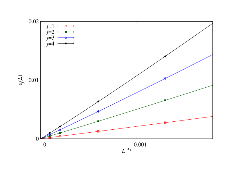
In order to do so, we consider all values of $j$ at the same time and perform a global fit, enforcing data from different zeros to share the same $x_{1}$ and $x_{2}$. As points coming from a given $L$ are correlated, the full covariance matrix has to be considered. We label our set of points $\{\epsilon_{j}(L_{a})\}$ by their $L$ and their $j$: we have data for $\mathcal{L}=5$ different values of $L$ ($L_{1}=8$, $L_{2}=12$, $L_{3}=16$, $L_{4}=24$, $L_{5}=32$) and for $j=1,2,3,4$. The appropriate goodness-of-fit estimator is, therefore,

$$\chi^{2}=\sum_{i,j=1}^{4}\sum_{a,b=1}^{\mathcal{L}}[\epsilon_{i}(L_{a})-A_{i}L_{a}^{-x_{1}}(1+B_{i}L_{a}^{-x_{2}})]\sigma_{(ia)(jb)}^{-1}[\epsilon_{j}(L_{b})-A_{j}L_{b}^{-x_{1}}(1+B_{j}L_{b}^{-x_{2}})],$$ (23)

where $\sigma_{(ia)(jb)}$ is the covariance matrix of the set of zeros (which is block diagonal, since data for different $L$ are uncorrelated).

Unfortunately, we do not have enough data to determine $x_{2}$ and $x_{1}$ at the same time (the resulting error in $\omega$ would be greater than $100\%$). Instead, we take $x_{2}=\omega=1.0(1)$ from [32] and fit only for $x_{1}$ and the amplitudes. The resulting fit for $L\geq 12$, shown in figure 1, gives

$$x_{1}=2.67(6)[1],\qquad\chi^{2}/\mathrm{d.o.f.}=5.88/7,$$ (24)

where the error in square brackets accounts for the uncertainty in $\omega$. Our determination of $x_{1}$ is now compatible with the expected value of $x_{1}=2.688(5)$. Therefore, the scaling of the zeros is consistent at the critical point.

5.2 Scaling in the low-temperature phase

Now we consider the scaling of $\epsilon_{j}(L)$ in the low-temperature phase. This time, we expect, from (13),

$$\epsilon_{j}(L)\simeq AL^{-x_{1}},$$ (25)

with $x_{1}=D$.

Figure 2: Scaling of the zeros at $\beta=1.4$, with a best fit to (25) for $L\geq 16$. We obtain $x_{1}=2.842(11)$, with $\chi^{2}/\mathrm{d.o.f.}=7.34/7$.

Figure 3: Scaling of the zeros at $\beta=1.2$, with a best fit to (25) for $L\geq 16$. We obtain $x_{1}=2.844(10)$, with $\chi^{2}/\mathrm{d.o.f.}=2.89/7$.

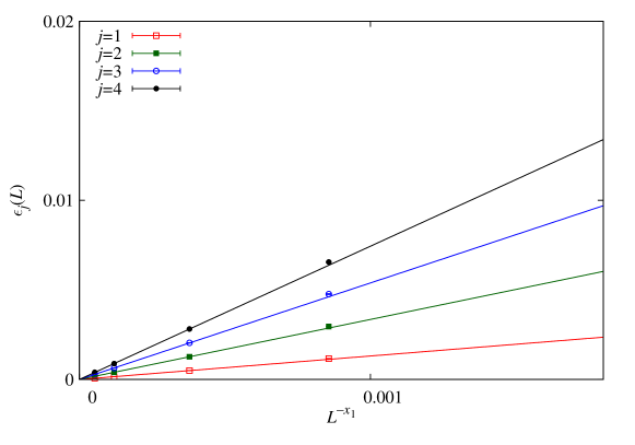
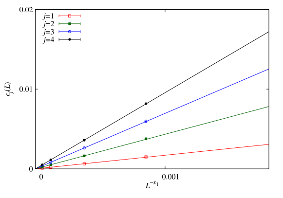
We have fitted the data for $\beta=1.2$ (Figure 3) and $\beta=1.4$ (Figure 3) to (25). The results, in Table 3, show a value of $x_{1}$ incompatible with $x_{1}=D=3$. We have also included corrections to scaling, using both $\omega=1$ (Goldstone-like correction) [34] and $\omega=3$ (Ising ordered correction) [34], $\omega=y=0.255$ (droplet) [35, 36, 37], $\omega=\theta(0)=0.39$ (replicon and also $1/\hat{\nu}$ which controls the scaling correction of $q_{\mathrm{EA}}(L)$ [21]), $\omega=0.79=2\theta(0)$ (twice the replicon [21]) and $\omega=0.65=\theta(q_{\mathrm{EA}})$ [21] but in neither case is the asymptotic $x_{1}=D$ behavior recovered (see Table 3). In addition, we have forced the fits with $x_{1}=3$ and leaving free $\omega$ and the statistical quality of the fits was bad.

Table 3: Scaling of the zeros in the low-temperature phase. For the two considered temperatures ($\beta=1.2,1.4$) we first show a fit without corrections to scaling for $L\geq 16$, that is $\epsilon_{j}(L)\simeq A_{j}L^{-x_{1}}$. As explained in Section 5.1, this is a global fit for the four zeros, considering their full covariance matrix. We then consider the same fit with corrections to scaling, trying different values for $\omega$ (see the text for more details). In all cases $x_{1}$ is smaller than the expected value $x_{1}=D=3$.

$L_{\mathrm{min}}$	$\beta$	$\omega$	$x_{1}$	$\chi^{2}/\mathrm{d.o.f.}$
16	1.4	-	2.842(11)	7.34/7
12	1.4	1	2.57(12)	3.79/7
12	1.4	3	2.79(2)	4.18/7
12	1.4	0.255	2.75(10)	17.6/7
12	1.4	0.39	2.67(9)	14.7/7
12	1.4	0.65	2.55(11)	7.90/7
12	1.4	0.79	2.48(13)	5.03/7
16	1.2	-	2.844(10)	2.89/7
12	1.2	1	2.82(5)	10.5/7
12	1.2	3	2.84(2)	6.90/7
12	1.2	0.255	2.80(10)	12.3/7
12	1.2	0.39	2.80(12)	11.9/7
12	1.2	0.65	2.81(10)	11.3/7
12	1.2	0.78	2.81(8)	11.0/7

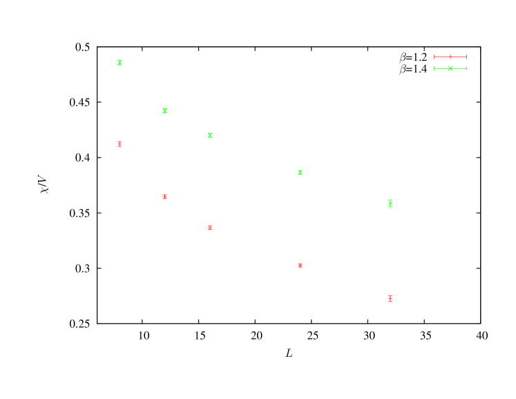
The origin of this discrepancy with the standard theory can be understood using Eq. 9. Notice from this equation that the scaling of the zeros depends strongly on the behavior of the non-connected spin glass susceptibility, so only with a divergence of this observable as the volume, we can recover $x_{1}=3$. However, for these two temperatures ($\beta=1.2$ and 1.4) this is not the case (see Fig. 4). Notice that $\overline{\langle q^{2}\rangle}=\chi/V$ has not reached the plateau asymptotic value: Hence at these temperatures the spin-glass susceptibility does not yet diverge as the volume.

Figure 4: $\chi/V=\overline{\langle q^{2}\rangle}$ versus the lattice size for $\beta=1.2$ and 1.4. Notice that none of the temperatures have reached the plateau asymptotic value.

5.3 Behavior of the integrated density of zeroes

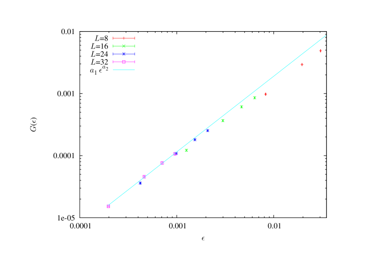
We will start our analysis of the integrated density of zeros by plotting this density at the critical point in Fig.5. One can see that the largest lattices follow a pure power law as predicted by the theory. The slope, on a log-log scale, of this straight line should correspond with an exponent $a_{2}$. Fitting only the $L=32$ points we obtain $a_{2}=1.16(2)$ in good agreement with the theory $a_{2}=1.116(2)$ (using Eq. 21 and $\eta=-0.375(10)$). To obtain this figure we have discarded in the fit the first zero.

For large $L$ we should expect a good collapse of all points in the same power law curve: the non collapsing part (small $L$ in the figure) is due to the presence of scaling corrections (which we also found in the previous sections).

Figure 5: Integrated density of zeros versus the zeros at the critical point. $a_{2}=1.16(2)$.

Figure 6: Integrated density of zeros versus the zeros for $\beta=1.2$.

Now we will check the theoretical predictions for the integrated density of zeros in the broken phase, which predict a linear behavior in the perturbing parameter $\epsilon$. Notice that in our case the margins between the critical point and the broken phase are tight since in the infinite volume limit we will see a behavior $\epsilon^{1.116}$ at the critical point which changes just below $T_{c}$ to $\epsilon$ (of course, this is due to the value of the $\eta$ exponent).

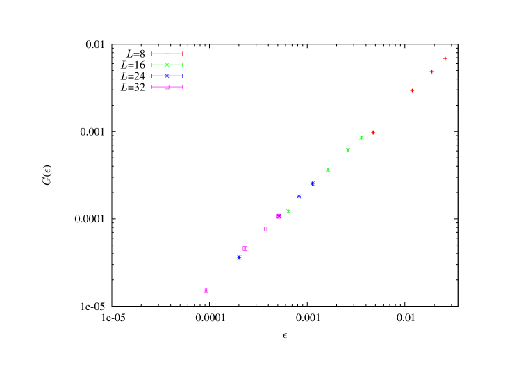
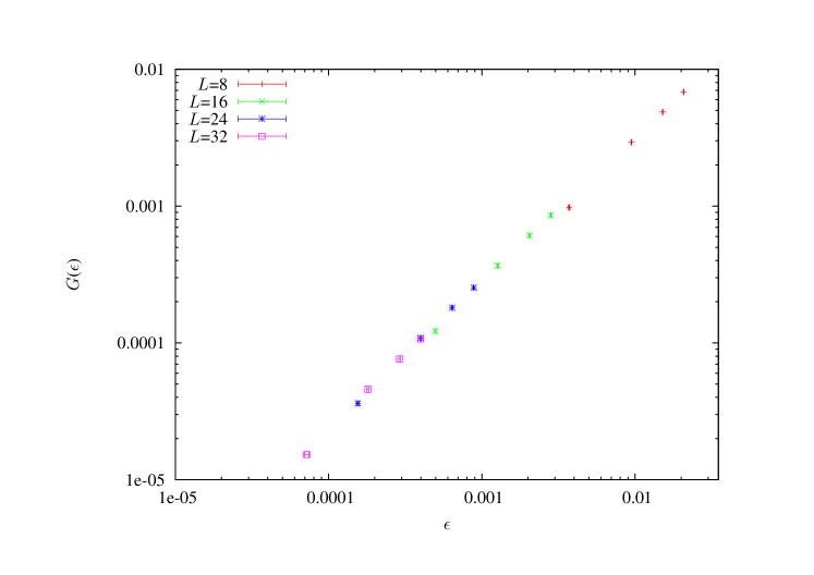
In Figs 6 and 7 we show that the data nearly follow a linear behavior of the integrated density deep in the spin glass phase (more concretely at $\beta=1.2$ and $\beta=1.4$), in particular for $L\geq 24$. The non-collapsing part of the curve is produced by the presence of scaling corrections as at the critical point.

Figure 7: Integrated density of zeros versus the zeros at $\beta=1.4$.

However, it is easy to show that if the zeros do not follow (for the lattice sizes simulated), in the broken phase, a scaling as the inverse of the volume, then the integrated density of zeros does not follow exactly a linear behavior, since $a_{2}=D/x_{1}$. We have discussed at the end of Sec. 5.2 that this lack of $1/V$ behavior is related to a susceptibility that is not yet diverging as the volume.

In sec. 5.2 we have found an exponent $x_{1}=2.842(11)$ for $\beta=1.2$ and $x_{1}=2.844(10)$ for $\beta=1.4$, which implies that $a_{2}=1.056(4)$ and $a_{2}=1.055(3)$ for $\beta=1.2$ and $\beta=1.4$ respectively.

Figure 8: Integrated density of the zeros, for the largest lattice $L=32$ and the lowest temperature $\beta=1.4$. Notice that we are almost, but not in, the linear regime. The data are well fitted with $b=1.068(10)$.

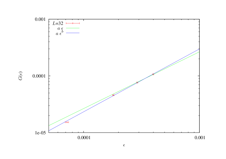
In Fig. 8 we show the behavior of the integrated density of zeros computed for our largest lattice ($L=32$) and lowest temperature, ($\beta=1.4$). Notice the points are not lying on a straight line. A fit to $a_{1}\epsilon^{a_{2}}$ works well, with $a_{2}$ consistent with the value computed from $x_{1}$ ($a_{2}=1.068(10)$). So we have obtained, numerically, $a_{2}=1.16(2)$, at the critical point which has changed to $1.068(10)$ in the broken phase.

Figure 9: Histogram ($N(\epsilon)$ versus $\epsilon$) for the 1000 first zeros computed for $L=32$ and $\beta=1.4$. Notice the lack of symmetry of the histogram and the presence of events for large values of the zeros.

Figure 10: Integrated density of the zeros, for the largest lattice $L=32$ and temperature $\beta=1.2$ using the average of zeros. We have also plotted the median values. We have marked the expected slope at the origin, using the Edwards-Anderson order parameter computed in Ref. [20] for the $L=32$ lattice.

Figure 11: Integrated density of the zeros, for the largest lattice $L=32$ and lowest temperature $\beta=1.4$ using the average of zeros. We have also plotted the median values. We have marked the expected slope at the origin, using the Edwards-Anderson order parameter computed in Ref. [20] for the $L=32$ lattice.

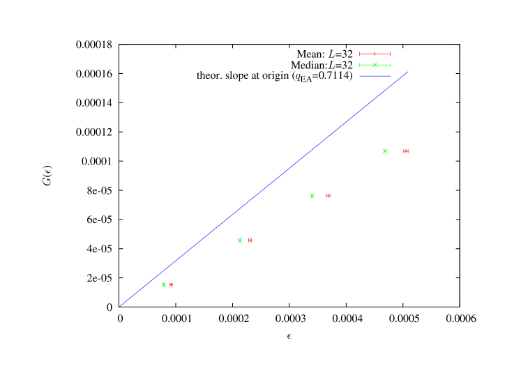
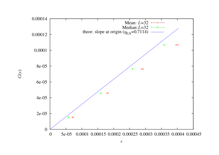
In this situation, we cannot compute the order parameter directly from the linear behavior of the integrated density since we are not observing a fully linear behavior. Hence, we confront our numerical data for $G(\epsilon)$ against the theoretical prediction for really small $\epsilon$, which is $G(\epsilon)=(\beta q_{\mathrm{EA}}/\pi)\epsilon$. It is interesting to note (see Refs. [27] and [34]) that we can recover the exact slope for a given lattice size if we substitute the value of the order parameter computed for this lattice size. We have followed this advice, and we show in Figs. 10 and 11 our data for $G(\epsilon)$ at $\beta=1.2$ and 1.4 showing $L=32$ data. In addition we have plotted the asymptotic slope using the order parameter ($q_{\mathrm{EA}}$) computed for $L=32$ lattices for these two temperatures in Ref. [20]. Notice that we have a slow approach to the right slope, but also that the overall picture seems to be correct.

In order to gain a better understanding of this effect, we have computed the density of zeros not with the average of the sample zeros but with the median of the probability distribution of the zeros.

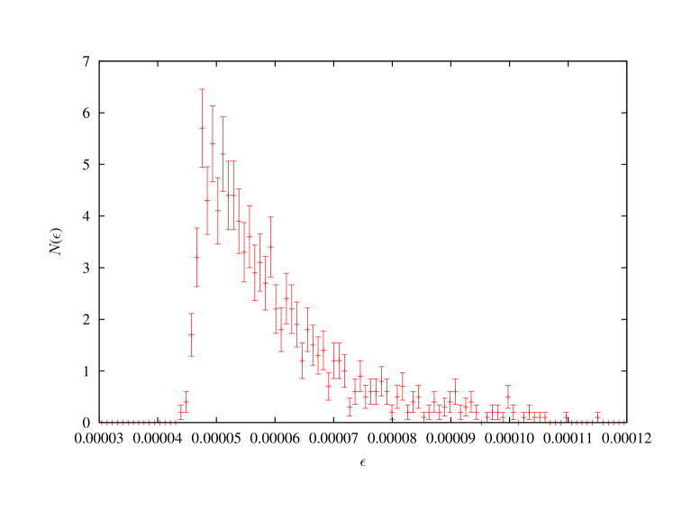
We show in Fig. 9 the histogram of the 1000 first zeros computed on the $L=32$ lattice at $\beta=1.4$. Notice from this figure the asymmetry of the histogram and the presence of events at large values of the zeros (which induces a large and strongly fluctuating value of the mean).

One can see in Figs. 10 and 11 that the median data produce an improved scaling, compared with those obtained from the mean, when comparing the data with the analytical prediction (slope provided by $q_{\mathrm{EA}}$).

For the sake of completeness, we can cite that the integrated density of zeros using the medians does not behave completely linearly but with a law $\epsilon^{1.06(2)}$ (for $\beta=1.4$).

6 Conclusions

By studying the complex singularities linked with the overlap we have obtained a clear picture of the critical region and of the low temperature phase fully compatible with that obtained by other more standard approaches.

In particular, we have studied the behavior of the individual zeros as well as the integrated density at the critical point. In both cases we have obtained good values for the $\eta$ exponent and we have seen that the data are compatible with the corrections to scaling published in the literature [32].

Finally, we have checked the scaling laws in the spin-glass phase, obtaining strong scaling corrections as found previously [20]. In addition we have obtained, by monitoring the behavior of the integrated density, a compatible picture using the zeros with that obtained from the order parameter of the model ($q_{\mathrm{EA}}$) computed in finite volumes with standard methods. We have also shown that the use of the median instead of the mean improves the overall picture.

References

- [1] Yang C N and Lee T D 1952 Phys. Rev. Lett. 87 410
- [2] Lee T D and Yang C N 1952 Phys. Rev. Lett. 87 410
- [3] Fisher M, in lectures in theoretical physics, vol 12, p 1. (University of Colorado Press, Boulder, 1965).
- [4] One S, Karaki Y, Suzuki M and Kawabata C 1968 J. Phys. Soc. Japan 54.
- [5] Falcioni M, Marinari E, Paciello M L, Parisi G and Taglienti B 1982 Phys. Lett. 108B 331
- [6] Marinari E 1984 Nucl. Phys. B235 123
- [7] Kenna R, Johnston DA and Janke W 2006 Phys. Rev. Lett. 96 115701
- [8] Ruiz-Lorenzo J J 1997 J. Phys. A 30 485
- [9] Kenna R and Ruiz-Lorenzo J J 2008 Phys. Rev. E 78 031134
- [10] Gordillo-Guerrero A, Kenna R and Ruiz-Lorenzo J J 2009 Phys. Rev. E 80 031135
- [11] Ozeki Y and Nishimori H 1988 J. Phys. Soc. Jpn. 57 1087
- [12] Damgaard P H and Lacki J 1995 Int. J. Mod. Phys. 6 819
- [13] Bhanot G and Lacki J 1993 J. Stat. Phys. 71 259
- [14] Saul L and Kardar M 1993 Phys. Rev. E 48 R3221
- [15] Matsuda Y, Müller M, Nishimori H, Obuchi T and Scardicchio A 2010 J. Phys. A: Math. and Theor. 43 285002
- [16] Takahashi K 2011 J. Phys.Math. and Theor. 44 235001
- [17] Matsuda Y, Nishimori H and Hukushima K 2008 J. Phys. A: Math. Theor. 41 324012
- [18] Hérisson D and Ocio M 2002 Phys. Rev. Lett. 88 257202 (Preprint arXiv:cond-mat/0112378)
- [19] Belletti F, Cruz A, Fernandez L A, Gordillo-Guerrero A, Guidetti M, Maiorano A, Mantovani F, Marinari E, Martin-Mayor V, Monforte J, Muñoz Sudupe A, Navarro D, Parisi G, Perez-Gaviro S, Ruiz-Lorenzo J J, Schifano S F, Sciretti D, Tarancon A, Tripiccione R and Yllanes D (Janus Collaboration) 2009 J. Stat. Phys. 135 1121
- [20] Baños R A, Cruz A, Fernandez L A, Gil-Narvion J M, Gordillo-Guerrero A, Guidetti M, Maiorano A, Mantovani F, Marinari E, Martin-Mayor V, Monforte-Garcia J, Muñoz Sudupe A, Navarro D, Parisi G, Perez-Gaviro S, Ruiz-Lorenzo J, Schifano S F, Seoane B, Tarancon A, Tripiccione R and Yllanes D (Janus Collaboration) 2010 J. Stat. Mech. P06026 (Preprint arXiv:1003.2569)
- [21] Baños R A, Cruz A, Fernandez L A, Gil-Narvion J M, Gordillo-Guerrero A, Guidetti M, Maiorano A, Mantovani F, Marinari E, Martin-Mayor V, Monforte-Garcia J, Muñoz Sudupe A, Navarro D, Parisi G, Perez-Gaviro S, Ruiz-Lorenzo J, Schifano S F, Seoane B, Tarancon A, Tripiccione R and Yllanes D (Janus Collaboration) 2010 Phys. Rev. Lett. 105 177202 (Preprint arXiv:1003.2943)
- [22] Belletti F, Cotallo M, Cruz A, Fernandez L A, Gordillo A, Maiorano A, Mantovani F, Marinari E, Martin-Mayor V, Monforte J, Muñoz Sudupe A, Navarro D, Perez-Gaviro S, Ruiz-Lorenzo J J, Schifano S F, Sciretti D, Tarancon A, Tripiccione R and Velasco J L (Janus Collaboration) 2008 Comp. Phys. Comm. 178 208–216 (Preprint arXiv:0704.3573)
- [23] Belletti F, Guidetti M, Maiorano A, Mantovani F Schifano S F, Tripiccione R, Cotallo M, Perez-Gaviro S, Sciretti D, Velasco J L, Cruz A, Navarro D, Tarancon A, Fernandez L A, Martin-Mayor V, Muñoz-Sudupe A, Yllanes D, Gordillo-Guerrero A, Ruiz-Lorenzo J J, Marinari E, Parisi G, Rossi M and Zanier G (Janus Collaboration) 2009 Computing in Science and Engineering 11 48
- [24] Baity-Jesi M, Banos R A, Cruz A, Fernandez L A, Gil-Narvion J M, Gordillo-Guerrero A, Guidetti M, Iniguez D, Maiorano A, Mantovani F, Marinari E, Martin-Mayor V, Monforte-Garcia J, Munoz Sudupe A, Navarro D, Parisi G, Pivanti M, Perez-Gaviro S, Ricci-Tersenghi F, Ruiz-Lorenzo J J, Schifano S F, Seoane B, Tarancon A, Tellez P, Tripiccione R and Yllanes D 2012 Eur. Phys. J. Special Topics 210 33 (Preprint arXiv:1204.4134)
- [25] Parisi G and Virasoro M 1989 J. Phys. I France 50 3317
- [26] Franz S, Parisi G and Virasoro M 1992 J. Phys. I France 2 1869
- [27] Janke W and Kenna R 2001 J. Stat. Phys. 102 1211
- [28] Janke W, Johnston D A and Kenna R 2004 Nucl. Phys. B 682 618
- [29] Hukushima K and Nemoto K 1996 J. Phys. Soc. Japan 65 1604 (Preprint arXiv:cond-mat/9512035)
- [30] Marinari E 1998 Optimized Monte Carlo methods Advances in Computer Simulation ed Kerstész J and Kondor I (Springer-Berlag)
- [31] Fernandez L A, Martin-Mayor V, Perez-Gaviro S, Tarancon A and Young A P 2009 Phys. Rev. B 80 024422
- [32] Hasenbusch M, Pelissetto A and Vicari E 2008 Phys. Rev. B 78 214205
- [33] Billoire A, Fernandez L A, Maiorano A, Marinari E, Martin-Mayor V and Yllanes D 2011 J. Stat. Mech. P10019 (Preprint arXiv:1108.1336)
- [34] Gordillo-Guerrero A, Kenna R and Ruiz-Lorenzo JJ (in preparation)
- [35] Carter A, Bray A J and Moore M A 2002 Phys. Rev. Lett. 88 077201
- [36] Boettcher S 2004 Europhys. Lett. 67 453
- [37] Boettcher S 2005 Phys. Rev. Lett. 95 197205
- [38] Fernandez L A, Gordillo-Guerrero A, Martin-Mayor V and Ruiz-Lorenzo J J 2008 Phys. Rev. Lett. 100 057201