Coarse grained models of stripe forming systems: phase diagrams, anomalies and scaling hypothesis

Abstract

Two coarse-grained models which capture some universal characteristics of stripe forming systems are studied. At high temperatures, the structure factors of both models attain their maxima on a circle in reciprocal space, as a consequence of generic isotropic competing interactions. Although this is known to lead to some universal properties, we show that the phase diagrams have important differences, which are a consequence of the particular $\vec{k}$ dependence of the fluctuation spectrum in each model. The phase diagrams are computed in a mean field approximation and also after inclusion of small fluctuations, which are shown to modify drastically the mean field behavior. Observables like the modulation length and magnetization profiles are computed for the whole temperature range accessible to both models and some important differences in behavior are observed. A stripe compression modulus is computed, showing an anomalous behavior with temperature as recently reported in related models. Also, a recently proposed scaling hypothesis for modulated systems is tested and found to be valid for both models studied.

I Introduction

Stripe forming systems are common in nature. Examples range from solid state systems, like ultrathin ferromagnetic films  DeMaWh2000 ; PoVaPe2003 , stress-induced submonolayer islands on several substrates MeLoAbBa2008 and strongly correlated electron systems KiFrEm1998 ; FrKi1999 , to soft matter systems like Langmuir monolayers SeMoGoWo1991 , block copolymers VeHaAnTrHuChRe2005 ; RuBoBl2008 , colloids and soft core systems MaPe2004 ; ImRe2006 ; GlGrKaKoSaZi2007 . The origin of stripe structures can be traced back to some strong universal mechanisms EdJa2010 . At the heart of stripe formation there is usually a competition between different kinds of interactions which lead to frustration and the formation of patterns or microphases. Common examples involve competition between a short range attractive interaction and a long range repulsion SeAn1995 .

Although several general properties of stripe forming systems are well known, as mean field phase diagrams and the behavior of the order parameter near the transition temperature Br1975 ; GaDo1982 ; BaRoFrGl1988 , the behavior at lower temperatures is less explored and new phenomena continue to appear. An example of this is the recently reported reentrance in the phase diagram of frustrated dipolar ferromagnets in an external magnetic field  SaLiPo2010 ; CaCaBiSt2011 .

These facts motivate us to look for a deeper understanding of the phase behavior of these kinds of systems. In the present work we address several questions which to a large extent remain open. We present a complete study of two very well known models of stripe forming systems, defined at a coarse-grain level, in which the main characteristic defining the phase behavior of the systems is the form of the effective spectrum of fluctuations, i.e. the wave vector dependence of the bare inverse correlation at low energies. This is known to determine the existence and type of phase transition, at least at mean field level. We define a coarse-grained free energy which is suitable for analyzing the low temperature behavior of relevant quantities, like magnetizations and modulation lengths, besides allowing the determination of the complete phase diagrams, in the whole temperature range. We show results from mean field approximation and also when fluctuations are taken into account. An efficient numerical implementation of the solutions allows us to compute several quantities with high accuracy.

The two models studied here are usually considered in the literature as yielding essentially the same physics. Instead, we show that besides obvious common characteristics, both models have very different phase diagrams and very different behaviors of important quantities, like the temperature dependence of modulation length. By introducing fluctuations to the mean field results we show that the nature of the transitions changes and the behavior of key quantities like magnetizations are drastically affected by fluctuations. An important characteristic of stripe forming systems with long range interactions is the temperature dependence of the modulation length and of the domain wall widths. We compute the T dependence of the modulation length in the whole T range, verify the well known square dependence near the transition and show that our analytic results compare very well with recent experimental data MeLoAbBa2008 down to low temperatures. We also introduce a measure of the width of domain walls and compare the T dependence of the width relative the behavior near the transitions, where a single mode approximation usually works fine. Finally, motivated by recent work on a scaling hypotesis for modulated systems PoGoSaBiPeVi2010 we compute a response function, the stripe compressibility, and show that it presents an anomalous behavior at low temperatures, in agreement with scaling predictions of systems with power law competing interactions. Interestingly, the general scaling behavior seems to work well also for a model which does not correspond to a system with long range interactions, our model 2 defined below. This points to a wider applicability of the proposed scaling hypotesis for stripe forming systems.

The paper is organized as follows: in Sec. II we introduce the coarse-grain free energy in terms of a generic spectrum of fluctuations. We define the equations of state at the mean field level and when fluctuations are included and show how to solve them in an efficient way. In Sec. III we introduce the two particular models studied, and present the main results on the phase diagrams and temperature dependence of several quantities. In Sec. IV we present the results of the stripe response function for both models. Finally, the conclusions of our work are discussed in Sec. V .

II Mean Field approach including fluctuations

We consider a generic model in two spatial dimensions defined by the coarse-grained free energy:

$$\mathcal{H}[\phi] = \frac{\gamma}{2a^{2}}\int d^{2}\vec{x}\,\left(\vec{\nabla}\phi\right)^{2}+\frac{1}{2\delta a^{2}}\int d^{2}\vec{x}\int d^{2}\vec{x^{\prime}}\ \phi(\vec{x}){J}(\vec{x}-\vec{x^{\prime}})\phi(\vec{x^{\prime}})+$$ (1)

$$\frac{1}{2\beta a^{2}}\int d^{2}\vec{x}\left\{\left(1+\frac{\phi(\vec{x})}{\phi_{0}}\right)\ln{\left(1+\frac{\phi(\vec{x})}{\phi_{0}}\right)}+\left(1-\frac{\phi(\vec{x})}{\phi_{0}}\right)\ln{\left(1-\frac{\phi(\vec{x})}{\phi_{0}}\right)}-2\ln{2}\right\}.$$

Here, $a$ represents the lattice spacing, $\beta=1/k_{B}T$ is the inverse temperature, $\gamma$ and $\delta$ are phenomenological constants and $\phi_{0}$ is the saturation value of the order parameter. The first term favors homogeneous configurations of the order parameter $\phi$ and the second term is intended to represent a competing force, represented by the kernel $J(\vec{x})$. These two terms can be considered the continuum limit of more microscopic competing interactions, as e.g. exchange and dipolar interactions in thin magnetic films GaDo1982 , hydrophobic and hydrophilic components in microemulsions or block copolymers BaRoFrGl1988 , or charge separation due to long range Coulomb forces in low dimensional electron systems FrKi1999 . The third term represents the mean field entropy. This effective Hamiltonian can be formally obtained. e.g. by a Hubbard- Stratonovich transformation BiDoFiNe1995 plus a coarse-grain process from an Ising model with competing short and long range interactions (represented by the non local term). A more common approach assumes an expansion of the entropy term for small $\phi$, which leads to the well known double well potential GaDo1982 ; BiDoFiNe1995 . We will consider instead the full form given by (1), which allows to compute the phase diagrams down to low temperatures.

Writing the quadratic part of (1) in reciprocal space and normalizing the order parameter field to its saturation value yields:

$$\mathcal{H}[\phi]=\frac{\phi_{0}^{2}}{2a^{2}}\int d^{2}\vec{k}\,A(\vec{k})\,\phi_{\vec{k}}\phi_{-\vec{k}}+\frac{1}{2\beta a^{2}}\int d^{2}\vec{x}\,\left\{\left(1+\phi(\vec{x})\right)\ln{\left(1+\phi(\vec{x})\right)}+\left(1-\phi(\vec{x})\right)\ln{\left(1-\phi(\vec{x})\right)}-2\ln{2}\right\},$$ (2)

where the spectrum of fluctuations is given by

$$A(\vec{k})=\gamma k^{2}+\frac{1}{2\delta}J(\vec{k}).$$ (3)

We consider systems in which the fluctuation spectrum has a single isotropic minimum at a non zero wave vector $k_{0}$. If $A(k_{0})<0$ the system will develop modulated structures. With some additional transformations it is possible to express the effective Hamiltonian in dimensionless form:

$$\frac{\mathcal{H}[\phi]}{E_{o}}=\int d^{2}\vec{k}\,{\hat{A}}(k)\,\phi_{\vec{k}}\phi_{-\vec{k}}+\frac{1}{\hat{\beta}}\int d^{2}\vec{x}\left\{(1+\phi(\vec{x}))\ln(1+\phi(\vec{x}))+(1-\phi(\vec{x}))\ln(1-\phi(\vec{x}))-2\ln{2}\right\},$$ (4)

where

$$E_{0} = \frac{\phi_{0}^{2}|A(k_{0})|k_{0}^{2}}{2a^{2}}$$

$$\hat{A}(k) = \frac{A(kk_{0})}{|A(k_{0})|}$$

$$\hat{\beta} = \phi_{0}^{2}|A(k_{0})|k_{0}^{4}\beta.$$ (5)

In this way all magnitudes but the characteristic energy $E_{0}$ in expression (4) are dimensionless . This expression was used for all the numerical computations in this work.

The mean field solutions of (4) are given by:

$$\left.\frac{\delta H[\phi]}{\delta\phi(\vec{x})}\right|_{\phi=\langle\phi\rangle}=0$$ (6)

Fluctuations to the mean field solution can be introduced in the form $\phi=\langle\phi\rangle+\psi$. The new stationary solutions are given by:

$$\left\langle\frac{\delta H[\langle\phi\rangle+\psi]}{\delta\langle\phi(\vec{x})\rangle}\right\rangle=0,$$ (7)

where the average is relative to the mean field measure.

II.1 Stripes solutions

It is well known that, in the absence of external fields, the solutions which minimize the free energy of model (4) are one dimensional modulations of the order parameter, i.e. stripe solutions in d=2, which can be written as:

$$\phi(x)=\sum_{i=0}^{\infty}m_{i}\sin\left(2\pi(2i+1)\frac{x}{\lambda}\right),$$ (8)

where $\lambda$ is the “modulation length”. In all calculations, the number of modes considered was $i_{max}=60$. This allow us to make a full characterization of the modulation profiles, as shown in the following sections.

The mean field equation (6) reads:

$$\phi(x)=\tanh\left[-\hat{\beta}\int\frac{d^{2}\vec{k}}{(2\pi)^{2}}e^{\mathit{i}\vec{k}\cdot\vec{x}}\hat{A}(k)\phi_{\vec{k}}\right]$$ (9)

To obtain the solution at a given temperature, equations (8) and (9) are solved for fixed $\lambda$. Then the free energy is minimized with respect to $\lambda$ to get the final solution.

II.2 Stripes solutions including fluctuations

Up to second order in the fluctuation fields, equation (7) is given by:

$$\frac{\delta H[\langle\phi\rangle]}{\delta\langle\phi(\vec{x})\rangle}-\frac{1}{\hat{\beta}}\frac{2\langle\psi^{2}\rangle(\vec{x})\langle\phi\rangle(\vec{x})}{(1-\langle\phi\rangle^{2}(\vec{x}))^{2}}=0$$ (10)

In order to solve this equation the mean squared local fluctuations $\langle\psi^{2}\rangle(\vec{x})$ have to be computed. To do this we used the following method: let’s consider the field $\phi(\vec{x})$ in the presence of a local unknown molecular field due to the rest of the system.

The partition function for a single site in an external field $h$ is:

$$Z(h)=\int_{-1}^{1}d\phi\,\exp{[-\beta H_{0}(h,\phi)]}$$ (11)

where

$${\beta}H_{0}(h,\phi) = -\beta h\phi+\frac{1}{2}\left[(1+\phi)\ln(1+\phi)\right.$$

$$+ \left.(1-\phi)\ln(1-\phi)-\ln{2}\right]$$

Then,

$$\langle\phi\rangle(h) = \frac{1}{Z(h)}\int_{-1}^{1}d\phi\ \phi\exp(-\beta H_{0}(h,\phi))$$

$$\langle\phi^{2}\rangle(h) = \frac{1}{Z(h)}\int_{-1}^{1}d\phi\ \phi^{2}\exp(-\beta H_{0}(h,\phi))$$

$$\langle\psi^{2}\rangle(h) = \langle\phi^{2}\rangle(h)-(\langle\phi\rangle(h))^{2}$$ (12)

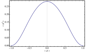
Of course, the value of the local molecular field $h$ remains unknown. Numerically, we can consider it as a free parameter to determine parametrically the non trivial relation between the mean square fluctuations $\langle\psi^{2}\rangle(\phi)$ and the mean local order parameter. The parametric solution of the system (12) is shown in Fig.1. It is important to note that, as a result of the temperature dependence of the potential used, the relation between $\langle\psi^{2}\rangle$ and $\langle\phi\rangle$ is temperature independent.

Figure 1: (Color on-line) Local relation between the fluctuations amplitude and the mean order parameter.

The equation of state including the fluctuation fields now reads:

$$\phi(x) = \tanh{\left[-\hat{\beta}\int\frac{d^{2}\vec{k}}{(2\pi)^{2}}e^{\mathit{i}\vec{k}\cdot\vec{x}}\hat{A}(k)\phi_{\vec{k}}\right.}$$ (13)

$$+ \left.\frac{2\psi^{2}(\phi(x))\phi(x)}{(1-\phi^{2}(x))^{2}}\right].$$

The effect of fluctuations is to add a new term in the effective field, which tends to rise up the order parameter profile in the region corresponding to domain walls. This means that when fluctuation effects are present profiles should be more sharp and correspondingly domain walls will be thinner.

In the following we apply the method described above to solve equations (9) and (13) for two well known models with stripe phases.

III Phase diagrams.

We focus our study in systems which present isotropic interactions, meaning that $\hat{A}(\vec{k})=\hat{A}(k)$. Due to our selection of dimensionless variables, the minimum of the fluctuation spectrum is reached at $k=1$ and then $\hat{A}(1)=-1$ . Besides these universal characteristics, different models are defined by the particular form of the fluctuation spectrum. The first model considered (model 1) is defined by Br1975 ; BaSt2007-1 ; CaCaBiSt2011 :

$$\hat{A}(k)=-1+a(k-1)^{2}$$ (14)

and the second (model 2) by HoSw1995 :

$$\hat{A}(k)=-1+a(k^{2}-1)^{2}.$$ (15)

Model 1 has a leading $\vec{k}$ dependence, for small $\vec{k}$, which is linear in $k\equiv|\vec{k}|$, i.e. it is non-analytic. It is a good model of, e.g. an ultrathin ferromagnetic film with strong perpendicular anisotropy, in which short range ferromagnetic exchange interaction competes with the long range dipolar interaction  PoGoSaBiPeVi2010 . Model 2 is known as the Swift-Hohemberg model, and was introduced to describe the physics at a convective instability SwHo1977 ; HoSw1995 . Alternatively, it can represent the continuum limit of a system with isotropic attractive nearest neighbors interactions plus repulsive next-nearest neighbor interactions  TeSt1987 ; DaLiWi1988 .

Although both models are similar in that they have a single minimum at a non zero wave vector modulus, they nevertheless show important differences which are shown in what follows . To our knowledge a detailed comparison of models of this kind has not been done up to now, and this frequently led to erroneous conclusions about their behavior.

III.1 Model 1

Fig. 2 shows the mean field phase diagram for model 1. The parameter $a$ is proportional to the curvature of the fluctuation spectrum at the minimum wave vector:

$$a=\frac{1}{2|{A(k_{0})}|}\left.\frac{d^{2}A(k)}{dk^{2}}\right|_{k=k_{0}}.$$ (16)

Note that, due to our choice of dimensionless variables, the temperature dependence is included in $\hat{\beta}$, defined as the inverse of $T/T_{c}$. This is the reason why the critical line is horizontal. This line defines a second order phase transition between a low temperature modulated phase and a high temperature disordered one.

Figure 2: (Color on-line) Mean field phase diagram for model 1. The dashed-dotted lines represent equal modulation length ($\lambda$) curves . The upper full line (blue on-line) corresponds to a second order transition between a modulated and a disordered phase. Dots represent the results of the numerical solution.

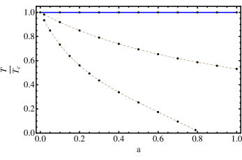
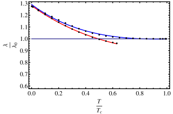
The dashed-dotted curves represent lines of constant modulation length $\lambda$. In fact, for fixed $a$ the modulation length decreases steadily as the temperature increases towards $T_{c}$ and then curves nearer the critical line correspond to smaller values of $\lambda$. The full temperature dependence of the modulation length is shown in Fig. 4 (dots), which shows that it varies continuously with temperature with an asymptotic value corresponding to the minimum of the spectrum.

Figure 3: (Color on-line) Mean field phase diagram for model 1 including fluctuations. The dashed- dotted lines represent equal modulation length ($\lambda$) curves . The upper full line (blue on-line) corresponds to a discontinuous transition between a modulated and a disordered phase. Dots represent the results of the numerical solution.

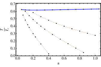
The phase diagram of model 1 including fluctuations is shown in Fig. 3. At first sight it seems similar to the mean field diagram. The critical temperature is depressed relative to the mean field one, as expected when fluctuations are included. The main difference with the mean field results is that the transition is discontinuous, i.e. fluctuations change the nature of the phase transition. In this case, the critical line was determined at the temperatures where the difference between the free energies of the disordered and modulated solutions changes sign. This characterizes a first order transition induced by fluctuations.

The behavior of the lines of constant modulation length is different from that of the mean field case. In Fig. 2 all the lines of constant $\lambda$ approach a limiting value of $\lambda=1$ at $T_{c}$, the value corresponding to the minimum of the spectrum $A(k)$, as can be seen in Fig. 4 (upper dots). When fluctuations are included the transition line is not an equal modulation length curve, in such a way that the modulation length at the transition point is a decreasing function of $a$.

While it is well known that the modulation length grows quadratically with temperature near the transition PoVaPe2006 ; CaCaBiSt2011 , the low temperature behavior of $\lambda$ is less known. Based on scaling approaches from other authors, Mentes et al. MeLoAbBa2008 proposed a numerical fit for their data on stripe forming ultrathin Pd/W(110) films. The proposed functionality, which takes into account fluctuation effects on the interface free energy and domain wall width, is the following:

$$\lambda(T)=\lambda_{0}+a(1-bT)\exp(-cT).$$ (17)

In Fig. 4 we show the results obtained directly from our numerical solutions (dots) together with the best fits from equation (17) (solid lines) for both approximations, mean field and mean field plus fluctuations, showing that the physically motivated form (17) is compatible with our numerical data.

Figure 4: (Color on-line) Temperature dependence of modulation length ($\lambda$) of model 1 for $a=1$, normalized to the value corresponding to the minimum of the spectrum, $\lambda_{0}$. Superior and inferior dots correspond to the results of the case without fluctuations and when fluctuations are included, respectively. The full lines represent the best fits of numerical results by the proposed functionality (17). The lower full line (red on-line) is interrupted because of the transition to the disordered phase.

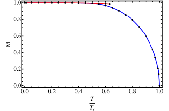
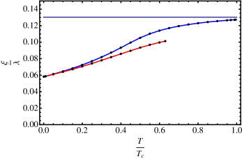
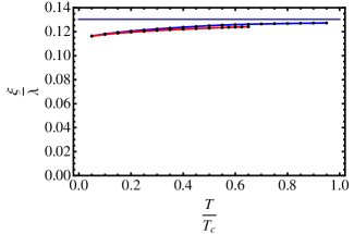
In figure 5 the behavior of the amplitude of the modulated solution is shown. The temperature in the horizontal axis is scaled relative to the critical temperature of the mean field solution. A notable fact is that the first order transition induced by fluctuations is very strong, the amplitude stays at very high values in the whole modulated phase, until the transition takes place. This is also reflected in the behavior of the domain wall width relative to the modulation length, which is shown in figure 6. The definition used for the domain wall width was

$$\xi=2\,\frac{\int_{0}^{\frac{\lambda}{4}}f(x)x\ dx}{\int_{0}^{\frac{\lambda}{4}}f(x)\ dx}$$ (18)

where the weight function $f(x)$ is $f(x)=M-\phi(x)$, and $M$ corresponds to the maximum value of the $\phi(x)$ profile. In our definition of $\phi(x)$ we fix the phase of the modulation, taking $\phi(0)=0$ and $\phi(x)$ positive in the interval $(0,\lambda)$. For example, for a sine like profile, the domain wall width is:

$$\frac{\xi}{\lambda}=\frac{\int_{0}^{\frac{\pi}{2}}(1-\sin(\theta))\theta d\theta}{\pi\int_{0}^{\frac{\pi}{2}}(1-\sin(\theta))d\theta}\approx 0.1303$$ (19)

This value would be a superior bound for the domain wall width, corresponding to the case of single mode approximation. In figures 6 and 11 this value was indicated by a horizontal line. We can see in each case how close profiles are of a sine function when the transition takes place.

Figure 5: (Color on-line) Temperature dependence of the modulation amplitude ($M$) for model 1 with $a=1$. The lower full line (blue on-line) corresponds to the mean field solution and the upper full one (red on-line) is the solution when fluctuations are included . Dots represent the results of the numerical solution.

Figure 6: (Color on-line) Temperature dependence of the domain wall width ($\xi$) normalized to the modulation length ($\lambda$) for model 1 with $a=1$. The superior full line (blue on-line) is the mean field solution and the lower one the solution with fluctuations included. The limit value of this magnitude for a perfect sine profile (single mode) is represented by the horizontal line. Dots represent the results of the numerical solution.

III.2 Model 2

The mean field phase diagram for model 2 is shown in Fig. 7. An important difference with respect to the corresponding diagram of model 1 is the presence of a uniform phase for small $T$ and $a$ values. This diagram has some similarity with phase diagrams of anisotropic models with short range competing interactions, like the ANNNI model RaReTa2010 . Nevertheless, at variance with the ANNNI model, in the present case there is no direct transition from the uniform to the disordered phases, at least up to very small values of $a$, where the precision of our algorithm breaks down. Instead, a sequence of two phase transitions with increasing temperature is observed. The modulated-uniform transition line characterizes a discontinuous transition at which the modulation length diverges, as can be seen in figure 8. Note that in the modulated region the free energy shows a single minimum at a finite modulation length $\lambda$, but as the temperature is lowered a second minimum at the far right of the figure appears. Numerically, this minimum is compatible with an infinite value of $\lambda$, typical of a homogeneous solution.

Figure 7: (Color on-line) Mean field phase diagram for model 2. The dashed-dotted lines represent equal modulation length ($\lambda$) curves . The full superior line (blue on-line) corresponds to a second order transition between a modulated and a disordered phase. The full lower line (red on-line) defines a transition between the modulated phase and a uniform phase. Dots represents the results of the numerical solution.

Figure 8: (Color on-line) Free energy of model 2 as a function of modulation length for different temperatures. Two top curves (blue on-line) show a single minimum at $\lambda$ slightly larger than 1. In the two curves at the bottom (green on-line) a second minimum to the right of the figure appears, signaling a discontinuous transition to a uniform state .

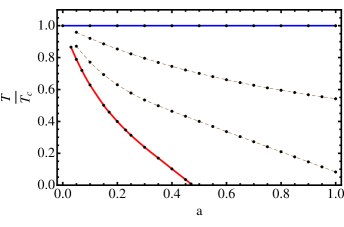
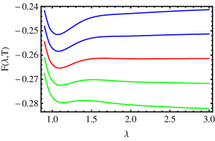
Figure 9 shows the phase diagram of model 2 when fluctuations to the mean field solution are included. As was the case for model 1, a first effect of fluctuations is to depress the transition line between the modulated and disordered lines.

The curves of constant $\lambda$ for model 2 in the mean field approximation are shown in Figure 7. They tend smoothly to the critical line, as in model 1 in such a way that higher curves corresponds to lower values of $\lambda$. The modulation length at the transition is a constant independent of $a$, corresponding to that of the minimum of the fluctuation spectrum. On the other hand when fluctuations are included the shape of the equal $\lambda$ curves changes, as shown in Figure 9. While upper curves still corresponds to lower values of the modulation length, in this case the modulation length at the transition is an increasing function of $a$, at variance with the behavior of model 1, where the modulation length at the transition is a decreasing function of the parameter $a$.

Figure 9: (Color on-line) Mean field phase diagram for model 2 including fluctuations. The dashed-dotted lines represent equal modulation length ($\lambda$) curves . The top line (blue on-line) corresponds to a second order transition to a disordered phase. Below the full bottom line (red on-line) a uniform phase has less free energy than the modulated one. Note the bending of the constant $\lambda$ curves, meaning an increasing modulation length with $a$ at the transition temperature. Dots represent the results of the numerical solutions.

In figure 10 the behavior of the modulation length with temperature is shown for model 2. Note that the values of $\lambda$ stay very near $\lambda_{0}$, the value at the transition, meaning that in the present model the modulation length has a weak dependence with temperature. This is an important difference with respect to the behavior of model 1. Nevertheless, as shown by the solid lines in the same figure, a fit to the expression (17) still works very well.

Figure 10: (Color on-line) Temperature dependence of modulation length ($\lambda$) for model 2 with $a=0.5$. Superior and inferior dots correspond to the results without fluctuations and when fluctuations are included, respectively. The full lines represent the best fits of numerical results by the proposed functionality (17). The lower line (red on-line) is interrupted because of the transition to the disordered phase..

The behavior of the domain wall width for model 2 is shown in figure 11. Comparing with figure 6 for model 1, we note that in the present model the profile is always very close to a sine, even at low temperatures. Besides that, fluctuations seem to be unimportant for the behavior of the domain wall width, at variance with the behavior observed in model 1. Nevertheless, the amplitude of the order parameter behaves similarly to that of model 1, staying practically at saturation until the transition temperature is reached, in the case when fluctuations are included. The fact that for model 2 the profiles stay very near the single mode case can be understood due to the presence of the quartic contribution in the fluctuation spectrum which implies that the energy required to excite higher harmonics at low temperatures is larger than in the quadratic case of model 1.

Figure 11: (Color on-line) Temperature dependence of the domain wall width ($\xi$) normalized to the modulation length ($\lambda$) for $a=0.5$ in model 2. The upper line (blue on-line) is the mean field solution and the lower one (red on-line) the solution with fluctuations included. The limit value of this magnitude for a perfect sine profile (single mode) is represented by the horizontal line. Dots represent the results of the numerical solution.

IV Anomalous behavior of stripe compressibility

A measure of a stripe compressibility in modulated systems can be obtained through the compression or Young modulus $B(T)$. This magnitude is related with the energy cost associated with deviations from the equilibrium modulation length ($\lambda(T)$) and it is defined as PoGoSaBiPeVi2010 :

$$B(T)=\lambda(T)^{2}\left.\frac{\partial^{2}F(\lambda,T)}{\partial\lambda^{2}}\right|_{\lambda(T)}$$ (20)

We calculated the compression modulus directly from the free energy $F(\lambda,T)$. In a recent work, Portmann et al. PoGoSaBiPeVi2010 have proposed some scaling relations for modulated matter. A scaling relation for the compression modulus was obtained in terms of the equilibrium modulation length ($\lambda(T)$) and the modulation amplitude ($M(T)$):

$$B=c\,M(T)^{2}\,\lambda(T)^{\Delta},$$ (21)

where $c$ is a constant and $\Delta$ is an exponent related with the system dimensionality and the microscopic nature of interactions. One of the main predictions of the proposed scaling relations is an anomalous behavior of the Young modulus when the exponent $\Delta$ is negative. This is the case, e.g. in a dipolar frustrated ferromagnet in two dimensions, which has an effective free energy of the type of model 1 in this work. More interestingly, Portmann and collaborators find the same form of scaling for the behavior of the critical magnetic field as a function of the modulation length PoGoSaBiPeVi2010 . This implies a reentrant or inverse transition in the external field vs temperature phase diagram at low temperatures for all systems which have a negative value of the exponent $\Delta$. This interesting result is supported by experimental measures in ultrathin films of Fe/Cu(001) from the same group SaLiPo2010 , and it has been reported in a Ginzburg-Landau model for the same system CaCaBiSt2011 .

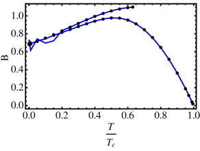
In Figures 12 and 13 we show the results of a direct calculation of the compression modulus (full curves) for both model 1 and model 2 via equation (20). The typical behavior of $B(T)$ in a normal system is a monotonically decreasing function of temperature, growing temperature leading to weaker bonds between particles and a weaker elastic response. However we can see in Figures 12 and 13 a regime for low enough temperatures where the compression modulus is an increasing function of temperature. Furthermore, the inclusion of fluctuations in both models do not destroy this behavior but strengthen the anomaly even more, which suggests a robust physics behind the numerical calculations. It is worth to mention that for very low temperatures the domain walls for model 1 become very sharp and as result numerical instabilities appear which can be seen in Figure 12.

We also tested the proposed scaling relation by fitting our analytical results with expression (21). Results are shown with dots in Figures 12 and 13. In all cases the proposed scaling law fits very well our numerical results. As part of our checking of the scaling predictions we let the initially fixed (quadratic) exponent of $M(T)$ in equation (21) to vary. The results for this exponent as well as for $\Delta$ in model 1 were very close to those predicted in PoGoSaBiPeVi2010 for the 2d dipolar frustrated ferromagnet. On the other hand, for model 2 important deviations where found. Nevertheless, in this case deviations for the values of exponents are expected because, strictly speaking, model 2 does not correspond to the kind of systems considered by Portmann and collaborators.

It is interesting that the scaling relations seem to be valid for a wider class of models. Future work should address the extension of the scaling relations to more general microscopic interactions as well as the origin of the anomalous behavior of the Young modulus in stripe forming systems.

Figure 12: (Color on-line) Continuous curves corresponds to the calculated Young modulus with and without fluctuations for model 1. The dots represent the best fit using the scaling relation equation (21).

Figure 13: (Color on-line) Continuous curves corresponds to the calculated Young modulus with and without fluctuations for model 2. The dots represent the best fit using the scaling relation equation (21).

V Conclusions

We have presented several new results regarding two well known effective models for stripe forming systems in two dimensions. The models can be thought as the continuous limits of some microscopic models with competing isotropic interactions, or alternatively, they can be defined directly through the form of the high temperature structure factor. A common feature of both models is that the structure factor has its maximum in a ring-like region in reciprocal space, which has strong consequences for the low temperature physics. Nevertheless, contrary to what is usually assumed in the literature, important differences were found in their properties and phase diagrams that lie in the specific wave vector dependende of the high-T structure factor, with Model 1 defined by a non-analytic dependence on the modulus of wave vector and Model 2 defined by an analytic form. Model 1 is a good small $k$ representation of some systems with long range interactions, like the dipolar frustrated ferromagnet and stripe forming systems with elastic interactions with the subtrate, while Model 2 can be obtained as an effective model for competing finite range isotropic interactions, which leads to an analytic expression for the $k$ dependence of the structure factor.

We have computed the full phase diagrams of both models in two approximations: mean field, and mean field plus fluctuations. Relevant equations were solved numerically. In both cases it is observed that fluctuations have a strong effect on the phase diagrams and other observables. With regard to phase diagrams, the main effect of fluctuations is to change the order of the isotropic to modulated phase transition from continuous in the mean field approximation to a strongly discontinuous transition when fluctuations are taken into account. Besides the isotropic-modulated transition, Model 2 shows another discontinuous phase transition from the modulated to a uniform (infinite modulation length) phase below a critical value of the parameter $a$, which characterizes the curvature of the fluctuation spectrum at the minimum.

In both models, the modulation length $\lambda$ is a smooth function of temperature, characterizing incommensurate modulations. The temperature dependence of $\lambda$ is strong for Model 1 and weak for Model 2. While in the mean field approximation the modulation length attains its mimimum value at the transition, which corresponds to the wave vector at the minimum of the structure factor, when fluctuations are taken into account $\lambda$ can take values less than that corresponding to the minimum of the structure factor. Another quantity of interest is the width of the domain walls $\xi$. We have introduced an operational definition of the width, taking as a reference value that corresponds to a single mode, sine-like solution, valid near the transition in the mean field approximation. As was the case with the modulation length, $\xi$ has a stronger dependence with temperature for Model 1. It is also important the fact that $\xi$ is smaller when fluctuations are included, meaning sharper domain walls, in line with the sharp phase transitions obtained in this case, where the amplitude of the modulations stay near saturation already below the transition.

Finally we have shown results for a response function, the compression modulus of stripes $B(T)$. This quantity shows an anomaly in its behavior, when compared with normal systems, having a maximum at intermediate temperatures. The anomalous behavior follows a recent prediction from a scaling hypothesis for modulated systems, which was obtained in the context of models with some particular long range interactions. We have verified its validity for both Model 1 and Model 2. Interestingly, although Model 2 does not belong to the kind of models for which the scaling hypothesis was predicted, it shows the same kind of scaling, with a particular scaling exponent. The scaling exponent for Model 1 corresponds, to a good numerical approximation, to the value predicted for a model with dipolar competing interactions.

In summary, we have computed some relevant quantities for models with modulated phases in two dimensions, complementing old results and clarifiying some differences between two models usually presented in the literature as giving essentially the same physics. We have shown that, despite the obvious similarities, both models have important differences. An interesting outcome of our results is the evidence of anomalous behavior in a response function in both models considered, in line with recent results in related models and experiments in ultrathin magnetic films. Future work should address the mechanisms that originate the anomalous behavior and the generality of this for other systems. Last but not least, the straightforward numerical implementation of the coarse-grained models defined in this work allowed us to access the whole temperature range of the phase diagrams, complementing already known results, usually limited to temperatures near the phase transition lines.